A collocation method of lines for two-sided space-fractional advection-diffusion equations with variable coefficients

Abstract

[Summary]We present the Method Of Lines (MOL), which is based on the spectral collocation method, to solve space-fractional advection-diffusion equations (SFADEs) on a finite domain with variable coefficients. We focus on the cases in which the SFADEs consist of both left- and right-sided fractional derivatives. To do so, we begin by introducing a new set of basis functions with some interesting features. The MOL, together with the spectral collocation method based on the new basis functions, are successfully applied to the SFADEs. Finally, four numerical examples, including benchmark problems and a problem with discontinuous advection and diffusion coefficients, are provided to illustrate the efficiency and exponentially accuracy of the proposed method.

, , , and , (2019), A collocation method of lines for two-sided space-fractional advection-diffusion equations with variable coefficients, Mathematical Methods in the Applied Sciences.

1 Introduction

Fractional Calculus (FC) started with some speculations of Leibniz and Euler, and it has been developed progressively up until now. The initial fundamental works on the subject of FC are gathered in the books of Miller and Ross ¹, Kilbas et al², Hilfer ³, Podlubny ⁴ and Kiryakova ⁵. Without any doubt, in today’s world, the concept of FC arises in many application’s fields. In fact, the recent developments of FC have shown that a large number of complex systems can be accurately modelled by ordinary and partial differential equations with fractional derivatives. These facts have created a new revolution of development in various fields of physics and engineering. ^{6, 7, 8}

In the last decade, fractional Advection-Diffusion Equations (ADEs) have received considerable attention in physics, mathematics and applications. A fractional ADE contains derivatives of fractional order in time, space or time-space. These three types of fractional ADEs have been used increasingly in the modelling of physical phenomena. Fractional ADEs are more proper for describing some phenomena such as anomalous diffusions, which arise in complex dynamics ⁹, transport of passive tracers carried by fluid flow in porous mediums ^{10, 11}, velocity of particle motion in blood flow or underground water ¹², etc. Various methods have been developed for solving fractional ADEs. We refer to some of them. Zheng et al¹³ used the finite element method to solve a space-fractional ADE with non-homogeneous initial-boundary conditions. Yang and Liu¹⁴ considered a numerical method for ADEs with Riesz space fractional derivatives on a bounded domain. Ding and Zhang¹⁵ presented a numerical technique for solving ADEs with Riesz space fractional derivatives. A homotopy analysis method were used to solve ADM with Riesz space fractional derivatives by Ray and Sahoo¹⁶. The Crank–Nicolson–Galerkin and backward Euler approximate schemes for two-dimensional space-fractional ADEs were investigated by Yanmin et al¹⁷. To solve ADE with two-sided space-time fractional derivative, a high-accuracy Legendre tau method is developed and a convergence analysis provided by Bhrawy and Zaky ¹⁸. A meshless method for solving time-fractional ADEs is considered by Tayebi et al¹⁹. Zhu et al²⁰ presented a differential quadrature method for solving time- and space- fractional ADEs. In the very recent paper ²¹, Li et al study fractional convection operators from physical and mathematical points of view and present a numerical scheme for space-fractional ADEs. As other numerical methods for fractional ADEs, we can refer to Zhai et al²², Bhrawy et al²³ and Li and Deng²⁴. For some numerical methods for other equations, which are relevant to fractional ADEs, we can refer the interested readers to Meerschaert and Tadjeran²⁵, Dehghan and Abbaszadeh²⁶, Feng et al^{27, 28}, Esmaeili²⁹, Zaky³⁰ and references therein.

Here, the following two-sided space-fractional ADE with variable coefficients is considered:

$$\frac{{\partial u(x,t)}}{{\partial t}}+\Big{(}{c_{\alpha}^{+}}(x,t){{}_{0}^{R}D_{x}^{\alpha}}+{c_{\alpha}^{-}}(x,t){{}_{x}^{R}D_{\ell}^{\alpha}}\Big{)}u(x,t)=\left({c_{\beta}^{+}}(x,t){{}_{0}^{R}D_{x}^{\beta}}+{c_{\beta}^{-}}(x,t){{}_{x}^{R}D_{\ell}^{\beta}}\right)u(x,t)+s(x,t),$$ (1a)

together with the initial and Dirichlet boundary conditions

$$u(x,0)=f(x),$$ (1b)

$$u(0,t)=u(\ell,t)=0.$$ (1c)

In Eq. (1a), the advection coefficients ${c_{\alpha}^{+}}(x,t)\geq 0$ and ${c_{\alpha}^{-}}(x,t)\geq 0$, and the diffusion coefficients ${c_{\beta}^{+}}(x,t)\geq 0$ and ${c_{\beta}^{-}}(x,t)\geq 0$, are some given functions, and ${{}_{0}^{R}D_{x}^{\sigma}}$ and ${{}_{0}^{R}D_{x}^{\sigma}}$ are the left- and right-sided Riemann–Liouville fractional derivatives of order $\sigma$, respectively. We remind that

$${}_{a}^{R}D_{x}^{\sigma}g(x) := \dfrac{1}{\Gamma(m-\sigma)}\dfrac{d^{m}}{dx^{m}}\int_{a}^{x}{(x-t)}^{m-\sigma-1}g(t)dt,$$

$${}_{x}^{R}D_{b}^{\sigma}g(x) := \dfrac{(-1)^{m}}{\Gamma(m-\sigma)}\dfrac{d^{m}}{dx^{m}}\int_{x}^{b}{(t-x)}^{m-\sigma-1}g(t)dt,$$

where $m$ is the integer number such that $m-1\leq\sigma<m$. It should be noted that the problem is considered on the domain $0<x<\ell$ and $0\leq t\leq T$. We consider the case $0<\alpha\leq 1$ and $1<\beta\leq 2$, where the parameters $\alpha$ and $\beta$ are the fractional orders (fractors) of the spatial variable. Moreover, the known function $s(x,t)$ is a source term.

We use the Method Of Lines (MOL) to solve problem (1). The MOL is one of the best methods for solving time-dependent partial differential equations numerically. It proceeds in two steps. In the first step, the spatial variable(s) are discretized by using one from various possible techniques, such as spectral, finite element, finite difference or meshless methods. In fact, the main idea of this method is to convert the partial differential equation to a system of initial values problems (IVPs). In the second step, a time integration method, such as a Runge–Kutta method, is utilized to solve the resulting system of IVPs. The MOL has been successfully applied to solve various types of problems in engineering and science.^{31, 32, 33, 34, 35}

In this paper, a suitable set of basis functions for spatial discretization is constructed by using Jacobi polynomials. Moreover, the right and left space-fractional derivatives of the basis functions are derived in closed form, which help us to simplify the spatial discretization of the problem. Then, the unknown solution is expanded in terms of the basis functions, and by using a collocation technique, the problem is reduced to an explicit system of IVPs. By solving this system of IVPs, an approximation for the solution of the problem is obtained.

In Section 2, we briefly review some of the standard definitions of Jacobi polynomials. The main aim of this paper is presented in Section 3, where we construct and develop our MOL for solving problem (1). In Section 4, some numerical examples are provided to show the efficiency of the proposed method. Some concluding remarks are provided at the end of the paper, in Section 5 of conclusion.

2 Preliminaries on Jacobi polynomials

One of the most practical classes of orthogonal polynomials on a closed interval $[-1,1]$ is the Jacobi polynomials, denoted by $P_{j}^{(a,b)}(x)$, $j=0,1,\ldots$. It is worthy to note that the Chebyshev, Legendre and Gegenbauer polynomials, are some important special cases of the Jacobi polynomials. The Jacobi polynomials have great flexibility to develop efficient numerical methods for solving a wide range of fractional differential models. Consequently, in the last decade, the Jacobi polynomials have been widely used to solve fractional problems. ^{36, 37, 38, 39, 40, 41, 42, 43} Our method uses the Jacobi polynomials too. Thus, in this section we briefly review the Jacobi polynomials, Jacobi quadrature rules, and a relevant theorem on the fractional derivatives of Jacobi polynomials.

An efficient formula for evaluating the Jacobi polynomials $P_{j}^{(a,b)}(x)$, $a,b>-1$, $x\in[-1,1]$, is given by the following three-term recurrence equation:

$$P_{0}^{(a,b)}(x):=1,\quad P_{1}^{(a,b)}(x):=\frac{1}{2}[(a+b+2)x+a-b],$$

$$P_{j+1}^{(a,b)}(x):=(A_{j}^{a,b}x-B_{j}^{a,b})P_{j}^{(a,b)}(x)-C_{j}^{a,b}P_{j-1}^{(a,b)}(x),\quad j=1,2,\ldots,m,$$

where

$$A_{j}^{a,b}:=\frac{(a+b+2j+1)(a+b+2j+2)}{2(j+1)(a+b+j+1)},$$ (2)

$$B_{j}^{a,b}:=\frac{(b^{2}-a^{2})(a+b+2j+1)}{2(j+1)(a+b+j+1)(a+b+2j)},$$

$$C_{j}^{a,b}:=\frac{(a+j)(b+j)(a+b+2j+2)}{(j+1)(a+b+j+1)(a+b+2j)}.$$

The Jacobi polynomials, with respect to the weight function $w^{(a,b)}(x):=(1-x)^{a}(1+x)^{b}$, are orthogonal:

$$\int_{-1}^{1}P_{j}^{(a,b)}(x)P_{i}^{(a,b)}(x)w^{(a,b)}(x)dx=\gamma_{j}^{a,b}\delta_{ij},$$ (3)

where

$$\gamma_{j}^{a,b}:=\frac{2^{a+b+1}\Gamma(j+a+1)\Gamma(j+b+1)}{(2j+a+b+1)j!\Gamma(j+a+b+1)}.$$ (4)

We remind the following two properties of the Jacobi polynomials, which are useful for our purposes:

$$P_{j}^{(a,b)}(-x)=(-1)^{j}P_{j}^{(b,a)}(x),$$ (5)

$$\frac{d^{m}}{dx^{m}}P_{j}^{(a,b)}(x)=d^{a,b}_{j,m}P_{j-m}^{(a+m,b+m)}(x),\qquad j\geq m\in\mathbb{N},$$ (6)

where

$$d^{a,b}_{j,m}:=\frac{\Gamma(j+m+a+b+1)}{2^{m}\Gamma(j+a+b+2)}.$$

The Jacobi polynomials satisfy the following important relation:

$$P_{k}^{(a,b-1)}\left(\frac{2x}{\ell}-1\right)=\frac{k+a+b}{2k+a+b}P_{k}^{(a,b)}\left(\frac{2x}{\ell}-1\right)+\frac{k+a}{2k+a+b}P_{k-1}^{(a,b)}\left(\frac{2x}{\ell}-1\right).$$ (7)

Since the Jacobi polynomials are orthogonal in $[-1,1]$, all zeros of $P_{m+1}^{(a,b)}(\tau)$ are simple and belong to the interval $(-1,1)$ ⁴⁴. These zeros are called the Jacobi–Gauss nodes with parameters $a$ and $b$, which we denote by $\{\xi^{(a,b)}_{i}\}_{i=0}^{m}$. It is worth mentioning that there is no closed-form formula to obtain the Jacobi–Gauss nodes. However, We can use stable and accurate methods to determine them ⁴⁴. The Jacobi–Gauss quadrature rule with parameters $a$ and $b$ is based on the Jacobi–Gauss nodes $\{\xi^{(a,b)}_{i}\}_{i=0}^{m}$ and can be used for approximating the integral of a function over the interval $[-1,1]$ with weight $(1-x)^{a}(1+x)^{b}$ as

$$\int_{-1}^{1}(1-x)^{a}(1+x)^{b}f(x)\text{d}x\simeq\sum_{i=0}^{m}\omega^{(a,b)}_{i}f(\xi^{(a,b)}_{i}),$$

where $\omega^{(a,b)}_{i}$, $i=0,\ldots,m$, are the Jacobi–Gauss quadrature weights, which are computed by

$$w_{i}^{(a,b)}:=\frac{2^{a+b+1}\Gamma(m+a+2)\Gamma(m+b+2)}{(m+1)!\Gamma(m+a+b+2)(1-x^{2}_{i})[(P_{m+1}^{(a,b)})^{\prime}(x_{i})]}.$$

The $(n+1)$-points Jacobi–Gauss quadrature rule is exact whenever $f(x)$ is a polynomial of degree less or equal than $2n+1$, i.e., in the Jacobi–Gauss quadrature rule, the degree of exactness is $2n+1$.

The following theorem plays a key role in establishing our method.

Theorem 2.1 (Zayernouri and Karniadakis⁴⁵).

Let $-1<b-\alpha<b$ and $b>0$. Then, for $x\in[0,\ell]$, we have

$${}_{0}^{R}D_{x}^{\alpha}\left[x^{b}P_{k}^{(a,b)}\left(\frac{2x}{\ell}-1\right)\right]=\frac{\Gamma(k+b+1)}{\Gamma(k+b-\alpha+1)}x^{b-\alpha}P_{k}^{(a+\alpha,b-\alpha)}\left(\frac{2x}{\ell}-1\right).$$

3 The proposed method of lines

The first step of our method consists to introduce appropriate basis polynomials (or functions) and expand the unknown solution in terms of them.

3.1 Modified Jacobi basis functions

A good choice of the basis functions is crucial from the numerical point of view. To do so, we begin by presenting a new set of basis functions and then some useful properties for them are given.

Definition 3.1.

Let $a,b>-1$. The Modified Jacobi Functions (MJFs) on $[0,\ell]$ are denoted by $\mathcal{J}^{(a,b,\rho,\theta)}_{k}(x)$, $k=0,1,\ldots$, and are defined as

$$\mathcal{J}^{(a,b,\rho,\theta)}_{k}(x):=x^{\rho}(\ell-x)^{\theta}\ P_{k}^{(a,b)}\left(\frac{2x}{\ell}-1\right),\ k=0,1,\ldots.$$

Remark 3.2.

It is worth to point out that our new class of MJFs is a generalization of the following four classes of well-known basis functions:

• if $\rho=\theta=0$ in Definition 3.1, then the classical Jacobi polynomials ⁴⁶ on $[0,\ell]$ are obtained;

• MJFs for $\theta=0$, $\rho=b=\alpha$, and $a=\alpha-q>-1$ are reduced to the basis functions presented in Esmaeili and Shamsi³⁶;

• MJFs for $\rho=b$, $\theta=0$, and $\theta=a$, $\rho=0$, are reduced to the Jacobi-polyfractonomials (or generalized Jacobi functions) ^{45, 47};

• MJFs for $\theta=a$ and $\rho=b$ are reduced to the basis functions defined in Mao and Karniadakis⁴⁸.

In the following, we give some simple but important properties of MJFs.

[Integer derivative] If $k$ is a positive integer number and $\rho,\theta>k$, $k=0,1,\ldots$, then

$$\frac{d^{k}}{dx^{k}}\mathcal{J}^{(a,b,\rho,\theta)}_{k}(x)\Big{|}_{x=0}=\frac{d^{k}}{dx^{k}}\mathcal{J}^{(a,b,\rho,\theta)}_{k}(x)\Big{|}_{x=\ell}=0.$$

For stable and accurate evaluation of MJFs, the following three-term recurrence relation is advised.

[Three-term recurrence relation] The MJFs satisfy the following recurrence relation:

$$\mathcal{J}^{(a,b,\rho,\theta)}_{0}(x)=x^{\rho}(\ell-x)^{\theta},\ \mathcal{J}^{(a,b,\rho,\theta)}_{1}(x)=\frac{1}{2}\left[(a+b+2)\left(\frac{2x}{\ell}-1\right)+a-b\right]\ x^{\rho}(\ell-x)^{\theta},$$

$$\mathcal{J}^{(a,b,\rho,\theta)}_{j+1}(x)=\left(A_{j}^{a,b}\left(\frac{2x}{\ell}-1\right)-B_{j}^{a,b}\right)\mathcal{J}^{(a,b,\rho,\theta)}_{j}(x)-C_{j}^{a,b}\mathcal{J}^{(a,b,\rho,\theta)}_{j-1}(x),\quad j=1,2,\ldots,m,$$

where $A_{j}^{a,b}$, $B_{j}^{a,b}$ and $C_{j}^{a,b}$ are defined in (2).

It is easy to verify that the MJFs are orthogonal with respect to the weight function.

[Orthogonality] The MJFs are orthogonal with respect to the weight function $w^{(a,b,\rho,\theta)}(x)$ as follows:

$$\int_{0}^{\ell}\mathcal{J}^{(a,b,\rho,\theta)}_{i}(x)\mathcal{J}^{(a,b,\rho,\theta)}_{j}(x)w^{(a,b,\rho,\theta)}(x)dx=\left(\frac{\ell}{2}\right)^{a+b+1}\gamma_{j}^{a,b}\delta_{ij},$$

where $w^{(a,b,\rho,\theta)}(x):=x^{b-2\rho}(\ell-x)^{a-2\theta}$ and $\gamma_{j}^{a,b}$ is defined in (4).

3.2 Spectral collocation method for spatial discretization

Now, we are in the position to discretize the spatial variable. For this purpose, we start to approximate the unknown function $u(x,t)$ in the problem (1) by $\tilde{u}_{n}(x,t)$ as follows:

$$u(x,t)\simeq\tilde{u}_{n}(x,t)=\sum_{k=0}^{n}a_{k}(t)\varphi_{k}(x),$$ (8)

where

$$\varphi_{k}(x):=\lambda_{k}\ \mathcal{J}^{(1,1,1,1)}_{k}(x)=\lambda_{k}x(\ell-x)P^{(1,1)}_{k}\left(\frac{2x}{\ell}-1\right)$$ (9)

and

$$\lambda_{k}:=\frac{1}{\ell^{3}}{\frac{\left(k+2\right)\left(2\,k+3\right)}{k+1}}.$$ (10)

It is interesting to point out that, in our collocation method, we choose $\varphi_{k}(x)$, $k=0,\ldots,n$, as the basis functions. We should mention that our motivation to use these basis functions is that they have some good features. First, they satisfy the boundary conditions (1c), thus $\tilde{u}_{n}(x,t)$ automatically satisfies the boundary conditions (1c). Second, as we will show in the next Subsection 3.3, the left and also right fractional derivatives of these basis functions can be obtained in a closed form, which simplifies the discretization stage.

Remark 3.3.

We note that, in order to improve the efficiency of the method, it is desirable that MJFs with $\rho,\,\theta\in(0,1)$ are considered as the basis function. However, by this consideration, we cannot derive both left and right derivatives in a closed form based on Jacobi polynomials. Accordingly, we develop our method with $\rho=\theta=1$.

Now, from (8), we can obtain the following approximations for $\tfrac{\partial}{\partial t}u$, ${}_{0}^{R}D_{x}^{\alpha}u$ and ${}_{0}^{R}D_{x}^{\beta}u$:

$$\frac{\partial}{\partial t}u(x,t)\simeq\frac{\partial}{\partial t}\tilde{u}_{n}(x,t)=\sum_{k=0}^{n}\dot{a}_{k}(t)\varphi_{k}(x),$$ (11)

$${}_{0}^{R}D_{x}^{\alpha}u(x,t)\simeq{}_{0}^{R}D_{x}^{\alpha}\tilde{u}_{n}(x,t)=\sum_{k=0}^{n}a_{k}(t)\psi_{k}^{\alpha+}(x),\quad{}_{0}^{R}D_{x}^{\beta}u(x,t)\simeq{}_{0}^{R}D_{x}^{\beta}\tilde{u}_{n}(x,t)=\sum_{k=0}^{n}a_{k}(t)\psi_{k}^{\beta+}(x),$$ (12)

$${}_{x}^{R}D_{\ell}^{\alpha}u(x,t)\simeq{}_{x}^{R}D_{\ell}^{\alpha}\tilde{u}_{n}(x,t)=\sum_{k=0}^{n}a_{k}(t)\psi_{k}^{\alpha-}(x),\quad{}_{x}^{R}D_{\ell}^{\beta}u(x,t)\simeq{}_{x}^{R}D_{\ell}^{\beta}\tilde{u}_{n}(x,t)=\sum_{k=0}^{n}a_{k}(t)\psi_{k}^{\beta-}(x),$$ (13)

where

$$\psi_{k}^{\alpha+}(x):={}_{0}^{R}D_{x}^{\alpha}\varphi_{k}(x),\qquad\psi_{k}^{\beta+}(x):={}_{0}^{R}D_{x}^{\beta}\varphi_{k}(x),$$ (14)

$$\psi_{k}^{\alpha-}(x):={}_{x}^{R}D_{\ell}^{\alpha}\varphi_{k}(x),\qquad\psi_{k}^{\beta-}(x):={}_{x}^{R}D_{\ell}^{\beta}\varphi_{k}(x).$$ (15)

Note that the computation of $\psi_{k}^{\alpha+}$, $\psi_{k}^{\beta+}$, $\psi_{k}^{\alpha-}$ and $\psi_{k}^{\beta-}$ are not straightforward. Thus, in the next Subsection 3.3, we present a novel method for evaluating them.

By substituting the approximations (11), (12) and (13) into Eq. (1a), we get

$$\sum_{k=0}^{n}\dot{a}_{k}(t)\varphi_{k}(x)+\left(c_{\alpha}^{+}(x,t)\sum_{k=0}^{n}a_{k}(t)\psi_{k}^{\alpha+}(x)+c_{\alpha}^{-}(x,t)\sum_{k=0}^{n}(-1)^{k}a_{k}(t)\psi_{k}^{\alpha-}(x)\right)\\ =\left(c_{\beta}^{+}(x,t)\sum_{k=0}^{n}a_{k}(t)\psi_{k}^{\beta+}(x)+c_{\beta}^{-}(x,t)\sum_{k=0}^{n}(-1)^{k}a_{k}(t)\psi_{k}^{\beta-}(x)\right)+s(x,t).$$ (16)

Let $\hat{\xi}_{i}^{(1,1)}$, $i=0,\ldots,n$, be the Jacobi–Gauss nodes associated with the interval $[0,\ell]$, which are defined as $\hat{\xi}_{i}^{(1,1)}:=\frac{\ell}{2}(\xi_{i}^{(1,1)}+1)$. By collocating (16) at $x=\hat{\xi}_{i}^{(1,1)}$, $i=0,\dots,n$, we arrive at

$$\sum_{k=0}^{n}\dot{a}_{k}(t)\varphi_{k}(\hat{\xi}_{i}^{(1,1)})+\left(c_{\alpha}^{+}(\hat{\xi}_{i}^{(1,1)},t)\sum_{k=0}^{n}a_{k}(t)\psi_{k}^{\alpha+}(\hat{\xi}_{i}^{(1,1)})+c_{\alpha}^{-}(\hat{\xi}_{i}^{(1,1)},t)\sum_{k=0}^{n}(-1)^{k}a_{k}(t)\psi_{k}^{\alpha-}(\hat{\xi}_{i}^{(1,1)})\right)\\ =\left(c_{\beta}^{+}(\hat{\xi}_{i}^{(1,1)},t)\sum_{k=0}^{n}a_{k}(t)\psi_{k}^{\beta+}(\hat{\xi}_{i}^{(1,1)})+c_{\beta}^{-}(\hat{\xi}_{i}^{(1,1)},t)\sum_{k=0}^{n}(-1)^{k}a_{k}(t)\psi_{k}^{\beta-}(\hat{\xi}_{i}^{(1,1)})\right)+s(\hat{\xi}_{i}^{(1,1)},t).\\$$

The above equations can be expressed in the following matrix form:

$$\mathbf{M}\,\dot{\mathbf{a}}(t)+\mathbf{C}^{+}_{\alpha}(t)\big{[}{\mathfrak{D}}^{+}_{\alpha}\ \mathbf{a}(t)\big{]}+\mathbf{C}^{-}_{\alpha}(t)\big{[}{\mathfrak{D}}^{-}_{\alpha}\ \mathbf{a}(t)\big{]}=\mathbf{C}^{+}_{\beta}(t)\big{[}{\mathfrak{D}}^{+}_{\beta}\ \mathbf{a}(t)\big{]}+\mathbf{C}^{-}_{\beta}(t)\big{[}{\mathfrak{D}}^{-}_{\beta}\ \mathbf{a}(t)\big{]}+\mathbf{s}(t),$$

where

$$\mathbf{M}:=\begin{bmatrix}\varphi_{0}(\hat{\xi}_{0}^{(1,1)})&\varphi_{0}(\hat{\xi}_{1}^{(1,1)})&\dots&\varphi_{0}(\hat{\xi}_{n}^{(1,1)})\\ \varphi_{1}(\hat{\xi}_{0}^{(1,1)})&\varphi_{1}(\hat{\xi}_{1}^{(1,1)})&\dots&\varphi_{1}(\hat{\xi}_{n}^{(1,1)})\\ \vdots&\vdots&\ddots&\vdots\\ \varphi_{n}(\hat{\xi}_{0}^{(1,1)})&\varphi_{n}(\hat{\xi}_{1}^{(1,1)})&\dots&\varphi_{n}(\hat{\xi}_{n}^{(1,1)})\\ \end{bmatrix},\quad\mathbf{a}(t):=\begin{bmatrix}a_{0}(t)\\ a_{1}(t)\\ \vdots\\ a_{n}(t)\end{bmatrix},\quad\mathbf{s}(t):=\begin{bmatrix}s(\hat{\xi}_{0}^{(1,1)},t)\\ s(\hat{\xi}_{1}^{(1,1)},t)\\ \vdots\\ s(\hat{\xi}_{n}^{(1,1)},t)\end{bmatrix},\quad$$

$$\mathbf{C}_{\alpha}^{+}(t):=\text{diag}\left(c_{\alpha}^{+}(\hat{\xi}_{0}^{(1,1)},t),\dots,c_{\alpha}^{+}(\hat{\xi}_{n}^{(1,1)},t)\right),\quad\quad\mathbf{C}_{\alpha}^{-}(t):=\text{diag}\left(c_{\alpha}^{-}(\hat{\xi}_{0}^{(1,1)},t),\dots,c_{\alpha}^{-}(\hat{\xi}_{n}^{(1,1)},t)\right),$$

$$\mathbf{C}_{\beta}^{+}(t):=\text{diag}\left(c_{\beta}^{+}(\hat{\xi}_{0}^{(1,1)},t),\dots,c_{\beta}^{+}(\hat{\xi}_{n}^{(1,1)},t)\right),\quad\quad\mathbf{C}_{\beta}^{-}(t):=\text{diag}\left(c_{\beta}^{-}(\hat{\xi}_{0}^{(1,1)},t),\dots,c_{\beta}^{-}(\hat{\xi}_{n}^{(1,1)},t)\right),$$

and

$${\mathfrak{D}}_{\alpha}^{+}:=\begin{bmatrix}\psi_{0}^{\alpha+}(\hat{\xi}_{0}^{(1,1)})&\psi_{1}^{\alpha+}(\hat{\xi}_{0}^{(1,1)})&\dots&\psi_{n}^{\alpha+}(\hat{\xi}_{0}^{(1,1)})\\ \psi_{0}^{\alpha+}(\hat{\xi}_{1}^{(1,1)})&\psi_{1}^{\alpha+}(\hat{\xi}_{1}^{(1,1)})&\dots&\psi_{n}^{\alpha+}(\hat{\xi}_{1}^{(1,1)})\\ \vdots&\vdots&\ddots&\vdots\\ \psi_{0}^{\alpha+}(\hat{\xi}_{n}^{(1,1)})&\psi_{1}^{\alpha+}(\hat{\xi}_{n}^{(1,1)})&\dots&\psi_{n}^{\alpha+}(\hat{\xi}_{n}^{(1,1)})\end{bmatrix},\quad{\mathfrak{D}}_{\alpha}^{-}:=\begin{bmatrix}\psi_{0}^{\alpha-}(\hat{\xi}_{0}^{(1,1)})&\psi_{1}^{\alpha-}(\hat{\xi}_{0}^{(1,1)})&\dots&\psi_{n}^{\alpha-}(\hat{\xi}_{0}^{(1,1)})\\ \psi_{0}^{\alpha-}(\hat{\xi}_{1}^{(1,1)})&\psi_{1}^{\alpha-}(\hat{\xi}_{1}^{(1,1)})&\dots&\psi_{n}^{\alpha-}(\hat{\xi}_{1}^{(1,1)})\\ \vdots&\vdots&\ddots&\vdots\\ \psi_{0}^{\alpha-}(\hat{\xi}_{n}^{(1,1)})&\psi_{1}^{\alpha-}(\hat{\xi}_{n}^{(1,1)})&\dots&\psi_{n}^{\alpha-}(\hat{\xi}_{n}^{(1,1)})\\ \end{bmatrix}.$$

By collocating the initial condition (1b) at $x=\hat{\xi}_{i}^{(1,1)}$, $i=0,\ldots,n$, we obtain that

$$\sum_{k=0}^{n}a_{k}(0)\varphi_{k}(\hat{\xi}_{i}^{(1,1)})=f(\hat{\xi}_{i}^{(1,1)}),\quad i=0,\ldots,n.$$

The above equations can be expressed in the following matrix form:

$$\mathbf{M}\,\mathbf{a}(0)=\mathbf{F},$$

where $\mathbf{F}:=[f(\hat{\xi}_{0}^{(1,1)}),f(\hat{\xi}_{1}^{(1,1)}),\ldots,f(\hat{\xi}_{n}^{(1,1)})]^{T}$ and $\mathbf{a}(0):=[a_{0}(0),a_{1}(0),a_{2}(0),\ldots,a_{n}(0)]^{T}$.

In summary, the main problem (1) is reduced to the following system of ordinary differential equations with initial condition:

$$[left=\empheqlbrace\,] \mathbf{M}\,\dot{\mathbf{a}}(t)=-\mathbf{C}^{+}_{\alpha}(t)\big{[}{\mathfrak{D}}^{+}_{\alpha}\ \mathbf{a}(t)\big{]}-\mathbf{C}^{-}_{\alpha}(t)\big{[}{\mathfrak{D}}^{-}_{\alpha}\ \mathbf{a}(t)\big{]}+\mathbf{C}^{+}_{\beta}(t)\big{[}{\mathfrak{D}}^{+}_{\beta}\ \mathbf{a}(t)\big{]}+\mathbf{C}^{-}_{\beta}(t)\big{[}{\mathfrak{D}}^{-}_{\beta}\ \mathbf{a}(t)\big{]}+\mathbf{s}(t),$$ (17a)

$$\mathbf{M}\mathbf{a}(0)=\,\mathbf{F}.$$ (17b)

If we compute the inverse of the mass matrix $\mathbf{M}$, then we can derive an explicit form of the above IVP. In the next theorem, we present the explicit form of the inverse of the mass matrix $\mathbf{M}$.

Theorem 3.4.

The mass matrix $\mathbf{M}$ is nonsingular and the $(i,j)$th entry of it can be obtained explicitly as

$$\left(\mathbf{M}^{-1}\right)_{i,j}=\frac{\ell\,w_{i}^{(1,1)}}{2(1-\xi_{i}^{(1,1)})(1+\xi_{i}^{(1,1)})}P_{j}^{(1,1)}\left(\xi_{i}^{(1,1)}\right),\quad i,j=0,1,\ldots,n,$$

where $w_{i}^{(1,1)},\ i=0,1,2,\ldots,n$, are the Gauss–Jacobi weights.

Proof 3.5.

To prove the theorem, it is sufficient to show that the inner product of the $i$th raw of $\mathbf{M}$ and the $j$th column of $\mathbf{M}^{-1}$ is equal to $\delta_{ij}$, i.e.,

$$\sum_{k=0}^{n}\varphi_{i}(\hat{\xi}_{k}^{(1,1)})\frac{\ell\,w_{k}^{(1,1)}}{2(1-\xi_{k}^{(1,1)})(1+\xi_{k}^{(1,1)})}P_{j}^{(1,1)}\left(\xi_{k}^{(1,1)}\right)=\delta_{ij},\quad i,j=0,\ldots,n.$$ (18)

To prove the above equations, we begin by using the orthogonality property (3), which allows us to write that

$$\int_{-1}^{1}P_{i}^{(1,1)}(x)P_{j}^{(1,1)}(x)(1-x)(1+x)dx=\frac{2^{3}(i+1)}{(2i+3)(i+2)}\delta_{ij},\quad i,j=0,\ldots,n.$$

By noting that $P_{i}^{(1,1)}(x)P_{j}^{(1,1)}(x)$ is a polynomial of degree at most $2n$, we conclude that the integral in the above equation can be computed exactly by using the Jacobi–Gauss quadrature rule based on the nodes $\{\xi_{j}\}_{j=0}^{n}$. In this way, from the above equation, we get

$$\sum_{k=0}^{n}w_{k}^{(1,1)}P_{i}^{(1,1)}(\xi_{k}^{(1,1)})P_{j}^{(1,1)}(\xi_{k}^{(1,1)})=\frac{2^{3}(i+1)}{(2i+3)(i+2)}\delta_{ij},\quad i,j=0,\ldots,n.$$

The above equations can be reformulated as

$$\sum_{k=0}^{n}\frac{\ell^{3}w_{k}^{(1,1)}}{2^{3}\hat{\xi}_{k}^{(1,1)}(\ell-\hat{\xi}_{k}^{(1,1)})}\frac{(2i+3)(i+2)}{\ell^{3}(i+1)}\hat{\xi}_{k}^{(1,1)}(\ell-\hat{\xi}_{k}^{(1,1)})P_{i}^{(1,1)}(\xi_{k}^{(1,1)})P_{j}^{(1,1)}(\xi_{k}^{(1,1)})=\delta_{ij}.$$

Using Eqs. (9)–(10) and by noting that $\xi_{k}^{(1,1)}=\frac{2\hat{\xi}_{k}^{(1,1)}}{\ell}-1$ and $\hat{\xi}_{k}^{(1,1)}(\ell-\hat{\xi}_{k}^{(1,1)})=\tfrac{\ell^{2}}{2^{2}}(1+\xi_{k}^{(1,1)})(1-\xi_{k}^{(1,1)})$, we arrive at Eq. (18) and thus the proof of the theorem is completed.

By using $\mathbf{M}^{-1}$, we can convert the implicit IVP (17) into the following explicit IVP:

$$[left=\empheqlbrace\,] \dot{\mathbf{a}}(t)=\mathbf{M}^{-1}\left[-\mathbf{C}^{+}_{\alpha}(t){\mathfrak{D}}^{+}_{\alpha}-\mathbf{C}^{-}_{\alpha}(t){\mathfrak{D}}^{-}_{\alpha}+\mathbf{C}^{+}_{\beta}(t){\mathfrak{D}}^{+}_{\beta}+\mathbf{C}^{-}_{\beta}(t){\mathfrak{D}}^{-}_{\beta}\right]\mathbf{a}(t)+\mathbf{M}^{-1}\mathbf{s}(t),$$ (19a)

$$\mathbf{a}(0)=\mathbf{M}^{-1}\,\mathbf{F}.$$ (19b)

By solving the above system of IVPs, with a well-developed time-marching method ⁴⁹, the unknown vector function $\mathbf{a}(t)$ is obtained numerically. Then, by using (8), an approximation of $u(x,t)$ is obtained.

3.3 On the computation of the left and right fractional derivatives of the basis functions

As we have seen, the fractional differentiation matrices ${{\mathbf{{\mathfrak{D}}}}}_{+}^{\alpha+}$, ${{\mathbf{{\mathfrak{D}}}}}_{+}^{\alpha-}$, ${{\mathbf{{\mathfrak{D}}}}}_{+}^{\beta+}$, and ${{\mathbf{{\mathfrak{D}}}}}_{+}^{\beta-}$ have a key role in our method. These matrices simplify the spatial discretization process by replacing the left and right fractional differentiations with matrix-vector products. To derive these matrices, we can use Eqs. (14) and (15). However, before it, we need to obtain the functions $\psi_{k}^{\alpha+}$, $\psi_{k}^{\alpha-}$, $\psi_{k}^{\beta+}$ and $\psi_{k}^{\beta-}$. At first glance, it seems that these functions can be easily obtained, by taking the analytical left/right fractional derivative of $\varphi_{k}(x)$. However, taking the analytical fractional derivative, especially for large $n$, is sophisticated. In this respect, in what follows, we present some theorems, which play key roles in obtaining the mentioned functions.

Theorem 3.6.

Let $\varphi_{k}(x)$, $k=0,1,\ldots$, be defined in (9) and $\psi_{k}^{\sigma+}(x):={}_{0}^{R}D_{x}^{\sigma}\varphi_{k}(x)$. Then, for the cases $0<\sigma<1$ or $1<\sigma<2$, we have

$$\psi_{0}^{\sigma+}(x)=\frac{6\Gamma(2)}{\ell^{2}\Gamma(2-\sigma)}x^{1-\sigma}-\frac{6\Gamma(3)}{\ell^{3}\Gamma(3-\sigma)}x^{2-\sigma},$$

and, for $k\geq 1$,

$$\psi_{k}^{\sigma+}(x)={x}^{1-\sigma}\left({\tfrac{\left(2\,k+3\right)\Gamma\left(k+3\right)}{\ell^{2}\left(k+1\right)\Gamma\left(k+2-\sigma\right)}}\hat{P}^{(1+\sigma,1-\sigma)}_{k}\left(x\right)-{\tfrac{\left(k+2\right)\Gamma\left(k+4\right)}{\ell^{3}\left(k+1\right)\Gamma\left(k+3-\sigma\right)}}{x}\hat{P}^{(1+\sigma,2-\sigma)}_{k}\left(x\right)-{\tfrac{\Gamma\left(k+3\right)}{\ell^{3}\Gamma\left(k+2-\sigma\right)}}{x}\hat{P}^{(1+\sigma,2-\sigma)}_{k-1}\left(x\right)\right).$$

When $\sigma=2$, we get

$$\psi_{0}^{2+}(x)=\frac{-12}{\ell^{3}},$$

$$\psi_{k}^{2+}(x)=\frac{\lambda_{k}}{\ell^{2}}\left((k+4)(k+3)x(\ell-x)\hat{P}^{(3,3)}_{k-2}\left(x\right)+2\ell(k+3)(\ell-2x)\hat{P}^{(2,2)}_{k-1}\left(x\right)-2\ell^{2}\hat{P}^{(1,1)}_{k}\left(x\right)\right),$$

where $\hat{P}^{(a,b)}_{k}\left(x\right):=\displaystyle P^{(a,b)}_{k}\left(\frac{2x}{\ell}-1\right)$.

Proof 3.7.

The evaluation of $\psi_{0}(x)$ is trivial. For $k\geq 1$, we have

$${\varphi_{k}}(x)=\lambda_{k}\left(\ell xP_{k}^{(1,1)}\left(\frac{2x}{\ell}-1\right)-x^{2}P_{k}^{(1,1)}\left(\frac{2x}{\ell}-1\right)\right),$$

and thus

$${}_{0}^{R}D_{x}^{\sigma}{\mathbf{\varphi_{k}}}(x)=\lambda_{k}\left(\;{}_{0}^{R}D_{x}^{\sigma}\left[\ell xP_{k}^{(1,1)}\left(\frac{2x}{\ell}-1\right)\right]-\;{}_{0}^{R}D_{x}^{\sigma}\left[x^{2}P_{k}^{(1,1)}\left(\frac{2x}{\ell}-1\right)\right)\right].$$ (20)

Using Theorem 2.1, one has

$$\;{}_{0}^{R}D_{x}^{\sigma}\left[\ell\,\lambda_{k}\,x\,P_{k}^{(1,1)}\left(\frac{2x}{\ell}-1\right)\right]=\frac{(2k+3)\Gamma(k+3)}{\ell^{2}(k+1)\Gamma(k+2-\sigma)}x^{1-\sigma}P_{k}^{(1+\sigma,1-\sigma)}\left(\frac{2x}{\ell}-1\right).$$ (21)

Moreover, using the property (7), with $a=1$ and $b=2$, we get

$$P_{k}^{(1,1)}\left(\frac{2x}{\ell}-1\right)=\frac{k+3}{2k+3}P_{k}^{(1,2)}\left(\frac{2x}{\ell}-1\right)+\frac{k+1}{2k+3}P_{k-1}^{(1,2)}\left(\frac{2x}{\ell}-1\right).$$ (22)

Multiplying both sides of (22) by $\lambda_{k}x^{2}$, and applying the left-side fractional derivative, we arrive at

$$\;{}_{0}D_{x}^{\sigma}\Big{[}\lambda_{k}x^{2}P_{k}^{(1,1)}\left(\frac{2x}{\ell}-1\right)\Big{]}=\lambda_{k}\;{}_{0}D_{t}^{\sigma}\left[x^{2}\left(\frac{k+3}{2k+3}P_{k}^{(1,2)}\left(\frac{2x}{\ell}-1\right)+\frac{k+1}{2k+3}P_{k-1}^{(1,2)}\left(\frac{2x}{\ell}-1\right)\right)\right].$$

Using Theorem 2.1 once again, we conclude that

$$\;{}_{0}D_{x}^{\sigma}\Big{[}\lambda_{k}x^{2}P_{k}^{(1,1)}\left(\frac{2x}{\ell}-1\right)\Big{]}=\frac{(k+2)\Gamma(k+4)}{\ell^{3}(k+1)\Gamma(k+3-\sigma)}x^{2-\sigma}P_{k}^{(1+\sigma,2-\sigma)}\left(\frac{2x}{\ell}-1\right)\\ +\frac{\Gamma(k+3)}{\ell^{3}\Gamma(k+2-\sigma)}x^{2-\sigma}P_{k-1}^{(1+\sigma,2-\sigma)}\left(\frac{2x}{\ell}-1\right).$$ (23)

The proof of this theorem is concluded by plugging Eqs. (21) and (23) into relation (20). When $\sigma=2$, the use of property (6) completes the proof.

The next theorem is an important result, which has a key role for us to obtain a closed form for the right Riemann–Liouville fractional derivatives of the considered basis functions.

Theorem 3.8.

Let $\sigma>0$ and $m-1\leq\sigma<m$. Then

$$\psi_{k}^{\sigma-}(x):={}_{x}^{R}D_{\ell}^{\sigma}\varphi_{k}(x)=(-1)^{m}\psi_{k}^{\sigma+}(\ell-x).$$ (24)

Proof 3.9.

We have

$$\psi_{k}^{\sigma-}(x):=_{x}^{R}D_{\ell}^{\sigma}\varphi_{k}(x)=\dfrac{(-1)^{m}}{\Gamma(m-\sigma)}\dfrac{d^{m}}{dx^{m}}\int_{x}^{\ell}{(t-x)}^{m-\sigma-1}\varphi_{k}(t)dt.$$

By applying the change of variable $t\rightarrow\ell-\tau$, we get

$$\psi_{k}^{\sigma-}(x)=-\dfrac{(-1)^{m}}{\Gamma(m-\sigma)}\dfrac{d^{m}}{dx^{m}}\int_{\ell-x}^{0}{(\ell-\tau-x)}^{m-\sigma-1}\varphi_{k}(\ell-\tau)d\tau$$

and, by noting that $\varphi_{k}(\ell-\tau)=\varphi_{k}(\tau)$, we conclude that

$$\psi_{k}^{\sigma-}(x) = (-1)^{m}\dfrac{1}{\Gamma(m-\sigma)}\dfrac{d^{m}}{dx^{m}}\int_{0}^{\ell-x}{(\ell-x-\tau)}^{m-\sigma-1}\varphi_{k}(\tau)d\tau$$

$$= (-1)^{m}\Big{[}{}_{0}^{R}D_{x}^{\sigma}\varphi_{k}(x)\Big{]}_{x\rightarrow\ell-x}$$

$$= (-1)^{m}\psi_{k}^{\sigma+}(\ell-x).$$

The proof is complete.

Theorem 3.8 states that to evaluate the right-sided fractional derivative of order $\sigma$ of $\varphi_{k}(x)$, we can use the left-sided fractional derivative of order $\sigma$ of $\varphi_{k}(x)$, then substitute $x$ by $\ell-x$ and, finally, multiply it by $(-1)^{m}$. This property is related with the concept of duality as introduced by Caputo and Torres ⁵⁰.

In summary, by the explicit formulas in Theorems 3.6 and 3.8, for functions $\psi_{k}^{\sigma+}$ and $\psi_{k}^{\sigma-}$, we can simply compute the elements of the matrices ${{\mathbf{{\mathfrak{D}}}}}_{+}^{\alpha+}$, ${{\mathbf{{\mathfrak{D}}}}}_{+}^{\alpha-}$, ${{\mathbf{{\mathfrak{D}}}}}_{+}^{\beta+}$, and ${{\mathbf{{\mathfrak{D}}}}}_{+}^{\beta-}$.

4 Numerical experiments

In this section we illustrate the proposed method of lines by using concrete numerical experiments. We have implemented our method using Matlab on a 3.5 GHz Core i7 PC with 8 GB of RAM. Moreover, to solve IVP (19), the solver ode45 was used. This solver is based on an explicit Dormand–Prince Runge–Kutta (4, 5) formula ^{51, 52}. By using a suitable error estimation, the solver generates an adaptive mesh $t_{0},\dots,t_{k}$ and obtains the values of the solution of IVP at this mesh. This formula is a single-step solver, i.e., in computing $\mathbf{a}(t_{k})$, it needs only the solution at the immediately preceding time point, $\mathbf{a}(t_{k-1})$. In ode45, we can adjust the accuracy of the solution through the input parameters AbsTol and RelTol. In our numerical experiments, we set AbsTol=$10^{-14}$ and RelTol=$10^{-12}$.

We consider four different examples. For the problems with a known exact solution, we assess the accuracy of our method by reporting the following $l_{2}$ and $l_{\infty}$ errors:

$$E_{2}(n) := \sqrt{\frac{1}{100n}\sum_{i=0}^{n}\sum_{j=0}^{100}\left(u(\hat{\xi}_{i},j\tfrac{T}{100})-\tilde{u}_{n}(\hat{\xi}_{i},j\tfrac{T}{100})\right)^{2}},$$

$$E_{\infty}(n) := \max\left\{\mid u(\hat{\xi}_{i},j\tfrac{T}{100})-\tilde{u}_{n}(\hat{\xi}_{i},j\tfrac{T}{100})\mid:i=0,\ldots,n,\ j=0,\ldots,100\right\}.$$

Example 1

For the first example, we consider problem (1) with the following data borrowed from Meerschaert and Tadjeran⁵³:

$$\alpha:=1.8,\quad\ell:=2,\quad T:=5,\quad f(x):=4\,\left(2-x\right)^{2}{x}^{2},$$

$${c_{\alpha}^{+}}(x,t)={c_{\alpha}^{+}}(x,t):=0,\quad{c_{\beta}^{+}}(x,t):=\Gamma(1.2){x^{1.8}},\quad{c_{\beta}^{-}}(x,t):=\Gamma(1.2){(2-x)^{1.8}},$$

$$s(x,t):=-\tfrac{4}{11}\,{{\rm e}^{-t}}\left(211\,{x}^{4}-844\,{x}^{3}+1300\,{x}^{2}-912\,x+192\right).$$

In this problem, ehe exact solution is

$$u_{\text{ex}}(x,t):=4\,{{\rm e}^{-t}}{x}^{2}\left(2-x\right)^{2}.$$

By applying the proposed MOL with $n=4$, the obtained approximated solution and the error function are plotted in Fig. 1. Moreover, the errors $E_{2}(n)$ and $E_{\infty}(n)$ for various values of $n$, together with their CPU times, are shown in Fig. 2. As plotted in Fig. 2 (left), the errors $E_{2}(n)$ and $E_{\infty}(n)$ decrease very rapidly until, in $n=4$, they take over about $1e-13$. It is noted that, for $n>4$, the round-off errors on computer prevent any further improvement. However, it is worthwhile to note that, for $n>4$, the errors remain about $1e-13$, which shows that the presented MOL is numerically stable.

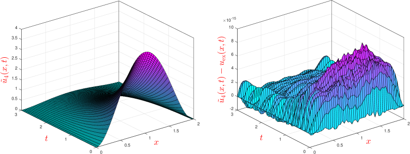
Figure 1: The approximate solution for Example 1 (left) together with the error function (right) obtained by the proposed method with $n=4$.

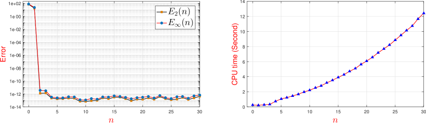
Figure 2: Errors $E_{2}(n)$ and $E_{\infty}(n)$ for Example 1 (left) for various values of $n$ together with their CPU times (right).

Example 2

For the second example, we consider problem (1) with the following data:

$$c_{\alpha}^{+}(x,t)=c_{\alpha}^{-}(x,t):=\frac{1}{\cos(\alpha\pi/2)},\quad c_{\beta}^{+}(x,t)=c_{\beta}^{-}(x,t):=\frac{-1}{\cos(\beta\pi/2)},\quad\ell=:1,\quad f(x):=0,$$

$$s(x,t):={\frac{24\,{t}^{\gamma}{{\rm e}^{\alpha\,t}}}{\cos\left(\alpha\pi/2\right)}\left({\frac{{x}^{2-\alpha}+\left(1-x\right)^{2-\alpha}}{12\,\Gamma\left(3-\alpha\right)}}-{\frac{{x}^{3-\alpha}+\left(1-x\right)^{3-\alpha}}{2\,\Gamma\left(4-\alpha\right)}}+{\frac{{x}^{4-\alpha}+\left(1-x\right)^{4-\alpha}}{\Gamma\left(5-\alpha\right)}}\right)}$$

$$\qquad\qquad\qquad+{\frac{24\,{t}^{\gamma}{{\rm e}^{\alpha\,t}}}{\cos\left(\beta\pi/2\right)}\left(\,{\frac{{x}^{2-\beta}+\left(1-x\right)^{2-\beta}}{12\,\Gamma\left(3-\beta\right)}}-{\frac{{x}^{3-\beta}+\left(1-x\right)^{3-\beta}}{2\,\Gamma\left(4-\beta\right)}}+{\frac{{x}^{4-\beta}+\left(1-x\right)^{4-\beta}}{\Gamma\left(5-\beta\right)}}\right)}$$

$$\qquad\qquad\qquad\qquad+{t}^{\gamma-1}{{\rm e}^{\alpha\,t}}\left(\alpha\,t+\beta\right){x}^{2}\left(1-x\right)^{2}.$$

The exact solution for this problem is

$$u_{\text{ex}}(x,t):={t}^{\gamma}{{\rm e}^{\alpha\,t}}{x}^{2}\left(1-x\right)^{2}.$$

This example is taken from Li et al²¹. In Table 1, we report the obtained results by applying the proposed method with $\gamma=2$ and some values of $\alpha$ and $\beta$. As it is seen, accurate results are obtained even by using a small $n$.

Table 1: The $l_{2}$ and $l_{\infty}$ errors for Example 2, obtained by the proposed method with $n=1,2,3$ and some values of $\alpha$ and $\beta$ with $\gamma=2$.

				$\beta=1.2$				$\beta=1.4$				$\beta=1.6$				$\beta=1.8$
$\alpha$		$n$		$E_{2}(n)$		$E_{\infty}(n)$		$E_{2}(n)$		$E_{\infty}(n)$		$E_{2}(n)$		$E_{\infty}(n)$		$E_{2}(n)$		$E_{\infty}(n)$
0.20		1		5.5e-03		4.6e-01		5.2e-03		4.6e-01		5.0e-03		4.6e-01		4.6e-03		4.5e-01
0.20		2		8.5e-14		1.4e-11		4.4e-14		7.9e-12		5.6e-14		1.1e-11		1.4e-14		3.0e-12
0.20		3		8.3e-14		1.4e-11		4.3e-14		7.8e-12		5.6e-14		1.1e-11		1.4e-14		3.0e-12
0.40		1		6.4e-03		5.6e-01		6.2e-03		5.6e-01		5.9e-03		5.6e-01		5.5e-03		5.4e-01
0.40		2		8.2e-14		1.4e-11		4.3e-14		8.0e-12		5.5e-14		1.1e-11		1.3e-14		3.0e-12
0.40		3		8.1e-14		1.4e-11		4.2e-14		7.8e-12		5.5e-14		1.1e-11		1.3e-14		3.0e-12
0.60		1		7.6e-03		6.8e-01		7.3e-03		6.9e-01		7.0e-03		6.8e-01		6.6e-03		6.7e-01
0.60		2		7.8e-14		1.3e-11		4.1e-14		7.6e-12		5.4e-14		1.1e-11		1.3e-14		3.0e-12
0.60		3		7.9e-14		1.4e-11		4.1e-14		7.9e-12		5.3e-14		1.1e-11		1.3e-14		2.9e-12
0.80		1		9.0e-03		8.4e-01		8.7e-03		8.4e-01		8.3e-03		8.4e-01		7.8e-03		8.2e-01
0.80		2		7.4e-14		1.3e-11		4.0e-14		7.7e-12		5.2e-14		1.1e-11		1.3e-14		2.9e-12
0.80		3		7.4e-14		1.3e-11		4.0e-14		7.7e-12		5.2e-14		1.1e-11		1.3e-14		2.9e-12

Example 3

In this example, we consider problem (1) with the data

$$c_{\alpha}^{+}=c_{\alpha}^{-}:=\frac{K_{\alpha}}{2\cos(\tfrac{\pi}{2}\alpha)},\quad c_{\beta}^{+}=c_{\beta}^{-}:=\frac{-K_{\beta}}{2\cos(\tfrac{\pi}{2}\beta)},\quad\ell:=\pi,\quad T:=4,\quad f(x):=\sin(4x).$$

This example, with $s(x,t):=0$ and different values of parameters $K_{\alpha}$ and $K_{\beta}$, is treated in Le et al²¹ and Yang et al¹⁴. When $s(x,t)=0$, the exact solution to this problem is, however, not known. For $\alpha=0.5$, $\beta=1.5$ and

$$s(x,t) :=2\,{{\rm e}^{-t}}\Bigg{\{}{\frac{2K_{\beta}}{\sqrt{2\,\pi-2\,x}\sqrt{\pi}}}-{\frac{\sqrt{2}K_{\beta}}{\sqrt{x\pi}}}-\frac{\sin\left(4\,x\right)}{2}$$

$$+\big{[}K_{\alpha}\sin\left(4x\right)-4K_{\beta}\cos\left(4x\right)\big{]}\texttt{FresnelS}\left(\sqrt{\tfrac{{8}}{{\pi}}x}\right)+\big{[}K_{\alpha}\sin\left(4x\right)+4K_{\beta}\cos\left(4x\right)\big{]}\texttt{FresnelS}\left(\sqrt{{{8-\tfrac{8}{\pi}x}}}\right)$$

$$+\big{[}K_{\alpha}\cos\left(4x\right)+4K_{\beta}\sin\left(4x\right)\big{]}\texttt{FresnelC}\left(\sqrt{\tfrac{8}{\pi}x}\right)-\big{[}K_{\alpha}\cos\left(4x\right)-4K_{\beta}\sin\left(4x\right)\big{]}\texttt{FresnelC}\left(\sqrt{8-\tfrac{8}{\pi}x}\right)\bigg{\}},$$

the exact solution of this problem is given by

$$u_{\text{ex}}(x,t):={{\rm e}^{-t}}\sin(4x).$$

We point out that FresnelC and FresnelS are the Fresnel cosine and Fresnel sine integral functions, respectively, which are defined as

$${\texttt{ FresnelC}}(x):=\int_{0}^{x}\cos\left(\frac{\pi\mu^{2}}{2}\right)\text{d}\mu,\qquad{\texttt{FresnelS}}(x):=\int_{0}^{x}\sin\left(\frac{\pi\mu^{2}}{2}\right)\text{d}\mu.$$

In contrast with the last two examples, here the exact solution is not a polynomial type function and thus this example is more proper for assessing the accuracy and convergence rate of our method. With this purpose, the errors $E_{2}(n)$ and $E_{\infty}(n)$ for various values of $n$ with $K_{\alpha}=2$ and $K_{\beta}=0.1$ are plotted in Fig. 3 (left). It can be observed from this figure that the errors decrease rapidly and the spectral convergence rate is gained by the method. Moreover, the obtained solution with $n=30$ and its corresponding error are plotted in Fig. 3 (right).

In addition, in order to show the effects of parameters $\alpha$, $\beta$, $K_{\alpha}$ and $K_{\beta}$, the obtained solutions for Example 3 with $s(x,t)=0$ are plotted in Fig. 4 for the parameter values of Table 2.

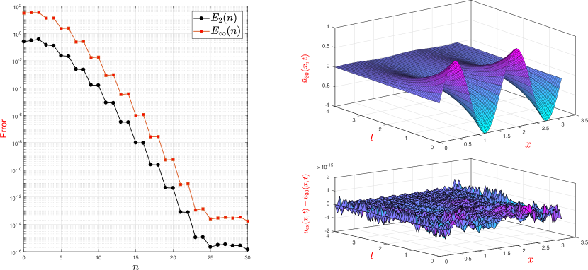
Figure 3: Example 3, with $\alpha=0.5$, $\beta=1.5$, $K_{\alpha}=2$ and $K_{\beta}=0.1$. Left: $E_{2}(n)$ and $E_{\infty}(n)$ for various values of $n$. Right: the obtained solution with $n=30$ and its corresponding error.

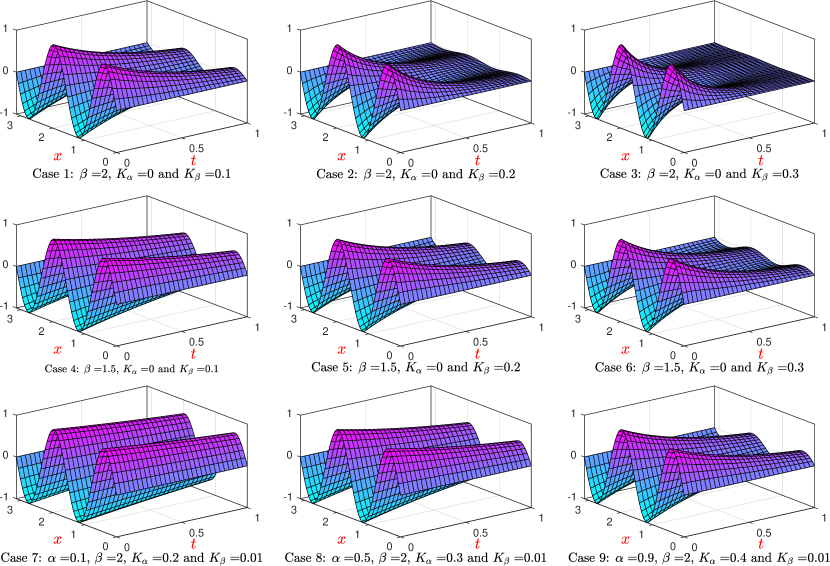
Figure 4: Obtained numerical solutions to Example 3 with $s(x,t)=0$ and various values of $\alpha$, $\beta$, $K_{\alpha}$ and $K_{\beta}$, for $n=50$.

Table 2: Different values of parameters $\alpha$, $\beta$, $K_{\alpha}$ and $K_{\beta}$ considered in Example 3 for problem with $s(x,t)=0$ (see Fig. 4).

	Case 1	Case 2	Case 3	Case 4	Case 5	Case 6	Case 7	Case 8	Case 9
$K_{\alpha}$	0.0	0.0	0.0	0.0	0.0	0.0	0.2	0.3	0.4
$\alpha$	-	-	-	-	-	-	0.1	0.5	0.9
$K_{\beta}$	0.1	0.2	0.3	0.1	0.2	0.3	0.01	0.01	0.01
$\beta$	2.0	2.0	2.0	1.5	1.5	1.5	2.0	2.0	2.0

Example 4

As a last example, we consider problem (1) with discontinuous data. Let

$$\ell:=7,\quad T:=1,\quad s(x,t):=0,\quad c_{\alpha}^{+}=c_{\alpha}^{-}:=1,\quad f(x):=\begin{cases}1,&1\leq x<2,\\ 2,&3\leq x<4,\\ 4,&5\leq x<6,\\ 0,&\text{otherwise},\end{cases}$$

and consider the diffusion coefficients in the following two cases:

$$\text{ Case I: }c_{\beta}^{+}=c_{\beta}^{-}:=\begin{cases}0.1,&0\leq x<4.5,\\ 0.001,&4.5\leq x\leq 7,\end{cases}\quad\text{ Case II: }c_{\beta}^{+}=c_{\beta}^{-}:=\begin{cases}0,&0\leq x<4.5,\\ 0.7,&4.5\leq x\leq 7.\end{cases}$$ (25)

By applying the proposed method with $n=200$ to the problem in Case I and Case II, the solutions are obtained after 3.1 and 3.2 seconds, respectively. These solutions are plotted in Fig. 5. As we can see, the obtained solutions are confirmed from a physical point of view. We conclude that the presented method can be applied with success to challenging problems with discontinuous data.

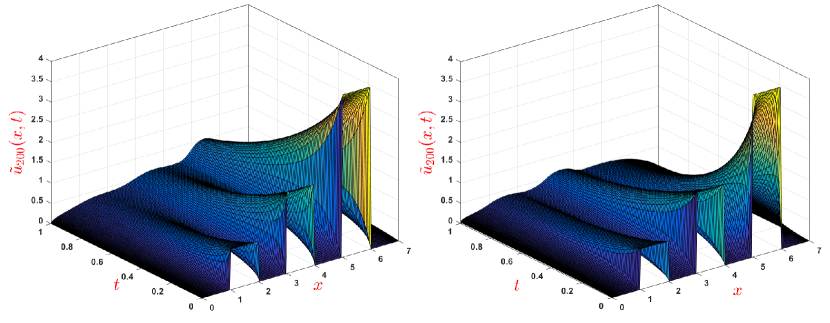
Figure 5: Approximate solutions obtained by the proposed method with $n=200$ for Example 4 in Cases I (left) and II (right) given by (25).

5 Conclusion

We proposed an efficient and accurate numerical method for solving two-sided space-fractional advection-diffusion equations. We started by introducing a new set of basis functions, called the Modified Jacobi Functions (MJFs). The method of lines, together with the spectral collocation method based on the introduced basis functions, were successfully applied to the considered problems. In order to increase the efficiency of the proposed method, from the numerical point of view, the left- and right-sided Riemann–Liouville fractional differentiation matrices were derived. Several numerical examples were provided, showing good efficiency and high accuracy (exponential accuracy). The obtained results confirm that our method not only works well for problems with smooth solutions (see Examples 1, 2 and 3) but also can be easily applied for problems with discontinuities on the initial condition, advection or diffusion coefficients (see Example 4). Obtaining some theoretical estimates for the approximation errors and convergence analysis would be desirable. This work is currently in progress. A further interesting topic for research is using MJFs, with $\rho,\,\theta\in(0,1)$, as the basis functions to solve the considered problem, by a Galerkin scheme.

References

- 1 Miller Kenneth S, Ross Bertram. An introduction to the fractional calculus and fractional differential equations. John Wiley & Sons; 1993.
- 2 Kilbas Anatoly A., Srivastava Hari M., Trujillo Juan J. Theory and applications of fractional differential equations North-Holland Mathematics Studies, vol. 204. Elsevier Science B.V., Amsterdam; 2006.
- 3 Hilfer R., ed. Applications of fractional calculus in physics. World Scientific Publishing Co., Inc., River Edge, NJ; 2000.
- 4 Podlubny Igor. Fractional differential equations Mathematics in Science and Engineering, vol. 198. Academic Press, Inc., San Diego, CA; 1999.
- 5 Kiryakova Virginia. Generalized fractional calculus and applications Pitman Research Notes in Mathematics Series, vol. 301. Longman Scientific & Technical, Harlow; copublished in the United States with John Wiley & Sons, Inc., New York; 1994.
- 6 West Bruce J. Fractional calculus and memory in biophysical time series. Fractals in Biology and Medicine. 2001;3:221–234.
- 7 Aparcana A., Cuevas C., Henríquez H., Soto H. Fractional evolution equations and applications. Mathematical Methods in the Applied Sciences. 2018;41(3):1256–1280.
- 8 Bazhlekova E. Estimates for a general fractional relaxation equation and application to an inverse source problem. Mathematical Methods in the Applied Sciences 2018;41(18):9018–9026.
- 9 Yang X.-J., Machado J.A.T. A new fractional operator of variable order: Application in the description of anomalous diffusion. Physica A: Statistical Mechanics and its Applications 2017;481:276–283.
- 10 Maqbool K., Anwar Bég O., Sohail A., Idreesa S. Analytical solutions for wall slip effects on magnetohydrodynamic oscillatory rotating plate and channel flows in porous media using a fractional Burgers viscoelastic model. European Physical Journal Plus. 2016;131(5):1–17.
- 11 Ali Abro K., Hussain M., Mahmood Baig M. An analytic study of molybdenum disulfide nanofluids using the modern approach of Atangana-Baleanu fractional derivatives. European Physical Journal Plus 2017;132(10).
- 12 Ahokposi D.P., Atangana A., Vermeulen D.P. Modelling groundwater fractal flow with fractional differentiation via Mittag-Leffler law. European Physical Journal Plus 2017;132(4).
- 13 Zheng Yunying, Li Changpin, Zhao Zhengang. A note on the finite element method for the space-fractional advection diffusion equation. Comput. Math. Appl. 2010;59(5):1718–1726.
- 14 Yang Q., Liu F., Turner I. Numerical methods for fractional partial differential equations with Riesz space fractional derivatives. Appl. Math. Model. 2010;34(1):200–218.
- 15 Ding Heng-Fei, Zhang Yu-Xin. New numerical methods for the Riesz space fractional partial differential equations. Comput. Math. Appl. 2012;63(7):1135–1146.
- 16 Ray S.S., Sahoo S. Analytical approximate solutions of Riesz fractional diffusion equation and Riesz fractional advection-dispersion equation involving nonlocal space fractional derivatives. Mathematical Methods in the Applied Sciences 2015;38(13):2840–2849.
- 17 Zhao Yanmin, Bu Weiping, Huang Jianfei, Liu Da-Yan, Tang Yifa. Finite element method for two-dimensional space-fractional advection-dispersion equations. Appl. Math. Comput. 2015;257:553–565.
- 18 Bhrawy A. H., Zaky M. A., Van Gorder R. A. A space-time Legendre spectral tau method for the two-sided space-time Caputo fractional diffusion-wave equation. Numerical Algorithms 2016;71(1):151–180.
- 19 Tayebi A., Shekari Y., Heydari M.H. A meshless method for solving two-dimensional variable-order time fractional advection-diffusion equation. Journal of Computational Physics 2017;340:655–669.
- 20 Zhu X. G., Nie Y. F., Zhang W. W. An efficient differential quadrature method for fractional advection–diffusion equation. Nonlinear Dynamics 2017;90(3):1807–1827.
- 21 Li Changpin, Yi Qian, Kurths Jürgen. Fractional convection. Journal of Computational and Nonlinear Dynamics 2018;13(1):011004.
- 22 Zhai Shuying, Feng Xinlong, He Yinnian. An unconditionally stable compact ADI method for three-dimensional time-fractional convection-diffusion equation. Journal of Computational Physics 2014;269:138–155.
- 23 Bhrawy A.H., Zaky M.A., Tenreiro Machado J.A. Efficient Legendre spectral tau algorithm for solving the two-sided space-time Caputo fractional advection-dispersion equation. JVC/Journal of Vibration and Control 2016;22(8):2053–2068.
- 24 Li C., Deng W. A New family of difference schemes for space fractional advection diffusion equation. Advances in Applied Mathematics and Mechanics 2017;9(2):282–306.
- 25 Meerschaert Mark M., Tadjeran Charles. Finite difference approximations for two-sided space-fractional partial differential equations. Appl. Numer. Math. 2006;56(1):80–90.
- 26 Dehghan M., Abbaszadeh M. A Legendre spectral element method (SEM) based on the modified bases for solving neutral delay distributed-order fractional damped diffusion-wave equation. Mathematical Methods in the Applied Sciences 2018;41(9):3476–3494.
- 27 Feng L.B., Zhuang P., Liu F., Turner I. Stability and convergence of a new finite volume method for a two-sided space-fractional diffusion equation. Applied Mathematics and Computation 2015;257:52–65.
- 28 Feng L.B., Zhuang P., Liu F., Turner I., Anh V., Li J. A fast second-order accurate method for a two-sided space-fractional diffusion equation with variable coefficients. Computers and Mathematics with Applications 2017;73(6):1155–1171.
- 29 Esmaeili S. Solving 2D time-fractional diffusion equations by a pseudospectral method and mittag-leffler function evaluation. Mathematical Methods in the Applied Sciences 2017;40(6):1838–1850.
- 30 Zaky Mahmoud A. A Legendre spectral quadrature tau method for the multi-term time-fractional diffusion equations. Computational and Applied Mathematics 2018;37(3):3525–3538.
- 31 Shakeri Fatemeh, Dehghan Mehdi. The method of lines for solution of the one-dimensional wave equation subject to an integral conservation condition. Comput. Math. Appl. 2008;56(9):2175–2188.
- 32 Dehghan Mehdi, Shakeri Fatemeh. Method of lines solutions of the parabolic inverse problem with an overspecification at a point. Numer. Algorithms 2009;50(4):417–437.
- 33 Schiesser William E. Method of lines PDE analysis in biomedical science and engineering. John Wiley & Sons, Inc., Hoboken, NJ; 2016.
- 34 Causley Matthew F., Cho Hana, Christlieb Andrew J., Seal David C. Method of lines transpose: high order L-stable schemes for parabolic equations using successive convolution. SIAM J. Numer. Anal. 2016;54(3):1635–1652.
- 35 Müller F., Schwab C. Finite elements with mesh refinement for elastic wave propagation in polygons. Mathematical Methods in the Applied Sciences 2016;39(17):5027–5042.
- 36 Esmaeili Shahrokh, Shamsi M. A pseudo-spectral scheme for the approximate solution of a family of fractional differential equations. Commun. Nonlinear Sci. Numer. Simul. 2011;16(9):3646–3654.
- 37 Esmaeili Shahrokh, Shamsi M., Luchko Yury. Numerical solution of fractional differential equations with a collocation method based on Müntz polynomials. Computers & Mathematics with Applications 2011;62(3):918–929.
- 38 Bhrawy A., Zaky M. A fractional-order Jacobi Tau method for a class of time-fractional PDEs with variable coefficients. Mathematical Methods in the Applied Sciences. 2016;39(7):1765–1779.
- 39 Bhrawy A.H., Zaky M.A. Shifted fractional-order Jacobi orthogonal functions: Application to a system of fractional differential equations. Applied Mathematical Modelling 2016;40(2):832–845.
- 40 Jahanshahi S., Babolian E., Torres D.F.M., Vahidi A.R. A fractional Gauss–Jacobi quadrature rule for approximating fractional integrals and derivatives. Chaos, Solitons & Fractals. 2017;102:295–304. arXiv:1704.05690
- 41 Kamali F., Saeedi H. Generalized fractional-order Jacobi functions for solving a nonlinear systems of fractional partial differential equations numerically. Mathematical Methods in the Applied Sciences 2018;41(8):3155–3174.
- 42 Izadkhah M.M., Saberi-Nadjafi J., Toutounian F. An extension of the Gegenbauer pseudospectral method for the time fractional Fokker-Planck equation. Mathematical Methods in the Applied Sciences 2018;41(4):1301–1315.
- 43 Zaky M.A., Doha E.H., Machado J.A. Tenreiro. A spectral framework for fractional variational problems based on fractional Jacobi functions. Applied Numerical Mathematics 2018;132:51–72.
- 44 Gautschi W. Orthogonal Polynomials: applications and computation. In: A. Iserles (Ed.), Acta Numerica, Cambridge Univ. Press; 1996.
- 45 Zayernouri Mohsen, Karniadakis George Em. Fractional Sturm-Liouville eigen-problems: theory and numerical approximation. J. Comput. Phys. 2013;252:495–517.
- 46 Shen Jie, Tang Tao, Wang Li-Lian. Spectral methods: algorithms, analysis and applications. Springer Science & Business Media; 2011.
- 47 Chen Sheng, Shen Jie, Wang Li-Lian. Generalized Jacobi functions and their applications to fractional differential equations. Math. Comp. 2016;85(300):1603–1638.
- 48 Mao Zhiping, Karniadakis George Em. A spectral method (of exponential convergence) for singular solutions of the diffusion equation with general two-sided fractional derivative. SIAM J. Numer. Anal. 2018;56(1):24–49.
- 49 Gladwell I. Numerical Solution of Ordinary Differential Equations (L. F. Shampine). SIAM Review. 1995;37(1):122–123.
- 50 Caputo M. Cristina, Torres D.F.M. Duality for the left and right fractional derivatives. Signal Processing 2015;107:265–271. arXiv:1409.5319
- 51 Dormand J.R., Prince P.J. A family of embedded Runge-Kutta formulae. Journal of Computational and Applied Mathematics 1980;6(1):19–26.
- 52 Shampine L. F., Gladwell I., Thompson S. Solving ODEs with MATLAB. Cambridge: Cambridge University Press; 2003.
- 53 Meerschaert Mark M., Tadjeran Charles. Finite difference approximations for fractional advection-dispersion flow equations. J. Comput. Appl. Math. 2004;172(1):65–77.