Longitudinal conductivity of hot magnetized collisional QCD medium in the inhomogeneous electric field

Abstract

The longitudinal current density induced by the inhomogeneous electric field in the hot magnetized quark-gluon plasma has been investigated and utilized in obtaining the conductivity of the medium. The analysis has been done in the regime where inhomogeneity of the field is small so that the collision effect could be significant. The modeling of the QCD medium is based on a quasiparticle description where the medium effects have been encoded in the effective quarks, antiquarks and gluons. The temperature dependence of the linear longitudinal current density (in terms of the electric field) and the additional components of current density due to the inhomogeneity of electric field (in terms of its derivatives) have been obtained by solving the $(1+1)-$dimensional effective covariant kinetic theory with a proper collision term. The conductivity has been obtained from the current density in the presence of the inhomogeneous field. The collisional aspects of the medium have been captured by including both thermal relaxation approximation and the Bhatnagar-Gross-Krook collision kernels in the analysis. Further, the hot QCD medium effects and higher Landau level contributions to the current density and the conductivity have been investigated. It has been seen that the effects of inhomogeneity of the field and the mean field corrections to the current density and the conductivity are more visible in the temperature regions which are not far from the transition temperature.

Keywords: Quark-gluon-plasma, Strong magnetic field, Inhomogeneous electric field, Thermal relaxation time, BGK collision kernel, Higher Landau levels.

PACS: 12.38.Mh, 13.40.-f, 05.20.Dd, 25.75.-q

I Introduction

Quantum chromodynamics (QCD) predicts a transition from normal hadronic matter to a deconfined state of matter called quark-gluon-plasma (QGP). The relativistically energetic heavy-ion collision experiments at Relativistic heavy-ion collider (RHIC) and large hadron collider (LHC), verified the existence of the QGP, as a near-perfect fluid STAR ; Aamodt:2010pb . Intense magnetic field has been created in the early stages of non-central asymmetric heavy-ion collisions and has great phenomenological significance Skokov:2009qp ; deng ; Zhong:2014cda ; Das:2016cwd ; Ghosh:2018xhh ; Mukherjee:2017dls ; Karmakar:2018aig ; Das:2017vfh ; Karmakar:2019tdp ; Bandyopadhyay:2017cle ; Koothottil:2018akg ; Roy:2017yvg ; Coci:2019nyr . Chiral magnetic effect Fukushima:2008xe ; Sadofyev:2010pr ; Huang ; She:2017icp , anomalous charge separation Huang:2015fqj , chiral vortical effect Kharzeev:2015znc ; Avkhadiev:2017fxj ; Yamamoto:2017uul and more recently, the realization of global $\Lambda$-hyperon polarization in RHIC STAR:2017ckg ; Becattini:2016gvu are some of the interesting aspects that are focus areas of current research on strong interaction physics at the RHIC. In addition, the intense magnetic field may affect the transport and thermodynamic properties of the QGP Hattori:2017qih ; Hattori:2016lqx ; Kurian:2018qwb ; Kurian:2017yxj ; Hattori:2016cnt ; Fukushima:2017lvb .

The quark and antiquark dynamics is described by $(1+1)-$dimensional Landau level (LL) kinematics (dimensional reduction) in the presence of the magnetic field Hattori:2017qih ; Kurian:2018dbn . The gluonic dynamics in the magnetized QGP can be indirectly affected through self-energy where quark/antiquark loop contributions are taken into account. The microscopic properties of Landau level dynamics of quarks, antiquarks result induce significant modifications to the macroscopic transport properties Hattori:2017qih ; Kurian:2018dbn . In the Refs Rath:2019vvi ; Li:2018ufq ; Feng:2017tsh ; Mohanty:2018eja ; Huang:2011dc ; Critelli:2014kra , the authors have investigated various transport coefficients in the presence of the magnetic field. Among them, conductivity is the most significant one, that describes the electromagnetic responses of the medium and controls the late time behaviour of electromagnetic fields. Inhomogeneous electromagnetic fields are expected to be generated in the heavy-ion collider experiments deng ; Tuchin:2013apa ; Hongo:2013cqa ; Tuchin:2012mf . The simplest component of current which is linear to the electric field is the Ohmic current. Since the inhomogeneity of the electromagnetic field has been already realized in heavy-ion collision experiments, it is an interesting task to investigate the additional components of the current due to the spacetime inhomogeneities of fields that are not negligible compared with the linear component while including the collisional effects. The longitudinal conductivity could be defined from the current itself. This sets the motivation for the current analysis.

The fluctuations of the electromagnetic field in the heavy-ion collision experiments might play significant role in understanding the electromagnetic responses of the medium. Recent investigations Zakharov:2017yst ; Tuchin:2013ie reveal that the fluctuations are much smaller as compared to the earlier predictions. In the current analysis, we are focusing on the regime where inhomogeneity of the electromagnetic field is small so that the collision effects cannot be neglected Satow:2014lia . For this purpose, proper collision integral for the processes that are dominant in the presence of a strong magnetic field need to be incorporated in the effective kinetic theory. The collisional aspects can be included either through relaxation-time approximation (RTA) or Bhatnagar-Gross-Krook (BGK) kernel. Recall that the quark-antiquark pair production and fusion processes are kinematically possible in the strong magnetic field limit Hattori:2016lqx . These processes are dominant over $2\rightarrow 2$ processes because of the fact that rate of the former one is proportional to the QCD running coupling constant $\alpha_{s}$ whereas that of binary processes is proportional to $\alpha_{s}^{2}$. In Ref. Kurian:2018qwb , authors computed the momentum dependent thermal relaxation time for the $1\rightarrow 2$ processes in the presence of the magnetic field. The collisional effects can also be described through BGK kernel. The difference between the BGK collisional term and the conventional relaxation RTA is that, the former case the number of particles is instantaneously conserved. Refs. Hattori:2016lqx ; Kurian:2017yxj ; Hattori:2016cnt describes the estimation of longitudinal current density (longitudinal conductivity) in the leading order in the presence of the strong magnetic field within the regime $T^{2}\ll\mid q_{f}B\mid$. Since the magnetic field is considerably strong in this regime, the thermal occupation of the higher Landau levels (HLLs) is suppressed exponentially as $e^{-\frac{\sqrt{q_{f}B}}{T}}.$ This allows to focus only on the lowest Landau level (LLL) state of quarks and antiquarks in the regime $T^{2}\ll\mid q_{f}B\mid$. Recent investigations Fukushima:2017lvb ; Kurian:2018qwb showed that the impact of HLLs are significant for the transport phenomena for an arbitrary magnetic field. The current analysis is on a more realistic regime $gT\ll\sqrt{\mid q_{f}B\mid}$ with full Landau level resummation.

The prime focus of the present analysis is to estimate the longitudinal current density of the magnetized QGP including the effects of inhomogeneity of electric field and HLLs, with proper collision term while incorporating the hot QGP medium interactions/effects. The analysis is done with the relativistic covariant kinetic theory by employing the effective fugacity quasiparticle model (EQPM) Chandra:2011en ; Mitra:2018akk . Hot QCD medium effects are incorporated in the EQPM quark/antiquark and gluonic degrees of freedom considering QGP as a Grand-canonical ensemble. Here, the current density picks up the mean field contribution from the local particle flow and energy-momentum conservation conditions within the effective kinetic theory. The mean field correction to the transport coefficients such as shear viscosity, bulk viscosity and thermal conductivity of a hot magnetized QGP is estimated in our previous work Kurian:2018qwb . In addition, one could read off the longitudinal conductivity from the current density. The temperature behaviour and magnetic field dependence of conductivity have also been investigated.

The manuscript is organized as follows. In section II, the mathematical formalism of the estimation of the longitudinal current density and conductivity in the hot QGP medium with the RTA and BGK kernel within the effective covariant kinetic theory is presented. Predictions of the effects due to inhomogeneity of field and HLLs in the current density and conductivity along with the mean field contributions are discussed in section III. Finally, in section IV the conclusion and outlook of the article are presented.

II Longitudinal conductivity of the QGP in the magnetic field

The inhomogeneity of the electric field generates the components of current in terms of spacetime derivatives of the field. The formalism for the estimation of the current density include the quasiparticle modeling of the QGP away from the equilibrium followed by the setting up of the effective covariant kinetic theory for the processes under consideration. The medium interactions are encoded in the quasiparticle models either through effective fugacity or effective mass parameter. The current analysis is done within the effective fugacity quasiparticle model (EQPM) Chandra:2011en ; Mitra:2018akk ; Chandra:2007ca ; Mitra:2017sjo , that encodes the ($2+1)-$flavor lattice equation of state (EoS) Cheng:2007jq ; Borsanyi . The temperature dependent quark and gluonic effective fugacities, $z_{q/\bar{q}}$ and $z_{g}$ respectively, describe the hot QCD medium interaction effects in the system. The extension of EQPM in the presence of the strong magnetic field is described in the Ref. Kurian:2017yxj .

For setting up the covariant effective kinetic theory within EQPM Mitra:2018akk in the presence of the strong magnetic field, we first need to define the basic macroscopic quantities of the system. We begin with the energy-momentum tensor $T^{\mu\nu}$ and particle four-flow $N^{\mu}(x)$ in the magnetized medium. The equilibrium energy-momentum tensor (longitudinal) in the presence of the strong magnetic field $\vec{B}=B\hat{z}$ can be defined in terms of quasiparticle momenta as follows Kurian:2018qwb ,

$$T^{\mu\nu}(x) =\sum_{l=0}^{\infty}\sum_{k=q,\bar{q}}\dfrac{\mid{q_{f}}_{k}B\mid}{2\pi}\mu_{l}N_{c}\int_{-\infty}^{\infty}{\dfrac{d{p}_{z_{k}}}{(2\pi)\omega_{l_{k}}}{p}_{k}^{\mu}{p}_{k}^{\nu}f^{0}_{k}(x,{p}_{z_{k}})}$$

$$+\sum_{l=0}^{\infty}\sum_{k=q,\bar{q}}\delta\omega\dfrac{\mid{q_{f}}_{k}B\mid}{2\pi}\mu_{l}N_{c}\int_{-\infty}^{\infty}{\dfrac{d{p}_{z_{k}}}{(2\pi){\omega_{l_{k}}}}\dfrac{\langle{p}_{k}^{\mu}{p}_{k}^{\nu}\rangle}{E_{l_{k}}}}$$

$$\times f^{0}_{k}(x,{p}_{z_{k}}).$$ (1)

In the local rest frame in which the hydrodynamic four-velocity $u^{\mu}=(1,{\bf 0})$, the quasiquark/antiquark momentum distribution function in the strong magnetic field has the following form,

$$f^{0}_{q}=\dfrac{z_{q}\exp{[-\beta(u^{\mu}\bar{p}_{\mu})]}}{1+z_{q}\exp{[-\beta(u^{\mu}\bar{p}_{\mu})]}}.$$ (2)

The quasiparticle dressed momenta $p^{\mu}$ can be defined in terms of bare particle momenta $\bar{p}^{\mu}$ through the dispersion relations as,

$$p^{\mu} =\bar{p}^{\mu}+\delta\omega u^{\mu}\equiv(\omega_{l},0,0,p_{z}), \delta\omega=T^{2}\partial_{T}\ln(z_{q}).$$ (3)

The dispersion relation that encodes the collective excitation of quasiparton modifies the zeroth component of the quasiparticle four-momenta in the local rest frame as,

$$\omega_{l}=E_{l}+\delta\omega,$$ (4)

in which $E_{l}\equiv\sqrt{p_{z}^{2}+m^{2}+2l\mid q_{f}B\mid}$ is the Landau levels of the quarks/antiquarks in the presence of magnetic field ($m_{u}=3$ MeV, $m_{d}=5$ MeV and $m_{s}=100$ MeV are the up, down and strange quarks masses respectively). Since the fermionic dynamics gets constrained to $(1+1)-$dimensional space, the longitudinal projection operator $\Delta_{\|}^{\mu\nu}$ in the dimensionally reduced space takes the form Li:2017tgi ,

$$\Delta_{\|}^{\mu\nu}\equiv g_{\|}^{\mu\nu}-u^{\mu}u^{\nu},$$ (5)

with $g_{\|}^{\mu\nu}=(1,0,0,-1)$. Here, $\langle p_{k}^{\mu}p_{k}^{\nu}\rangle=\dfrac{1}{2}(\Delta_{\|}^{\mu\alpha}\Delta_{\|}^{\nu\beta}+\Delta_{\|}^{\mu\beta}\Delta_{\|}^{\nu\alpha})p_{\alpha}p_{\beta}$. The integration phase factor in the strong magnetic field due to the dimensional reduction Bruckmann:2017pft ; Tawfik:2015apa ; Gusynin:1995nb is defined as,

$$\int{\dfrac{d^{3}p}{(2\pi)^{3}}}\rightarrow\dfrac{\mid q_{f}B\mid}{2\pi}\int_{-\infty}^{\infty}{\dfrac{dp_{z}}{2\pi}}\mu_{l},$$ (6)

with the Landau level degeneracy factor $\mu_{l}=(2-\delta_{l0})$. The energy-momentum tensor Eq. (II) gives the exact form of longitudinal pressure ($P_{\|}$) and energy density ($\varepsilon_{\|}$) in the strong magnetic field as described in Kurian:2017yxj , from the macroscopic description,

$$T^{\mu\nu}=\varepsilon_{\|}u^{\mu}u^{\nu}-P_{\|}\Delta_{\|}^{\mu\nu},$$ (7)

from which $\varepsilon_{\|}=u_{\mu}u_{\nu}T^{\mu\nu}$ and $P_{\|}={\Delta_{\|}}_{\mu\nu}T^{\mu\nu}$ can be defined.

Following the same arguments the particle four flow $N^{\mu}$ of the magnetized medium takes the following form,

$$N^{\mu}(x) =\sum_{l=0}^{\infty}\sum_{k=q,\bar{q}}\dfrac{\mid{q_{f}}_{k}B\mid}{2\pi}\mu_{l}N_{c}\int_{-\infty}^{\infty}{\dfrac{d{p}_{z_{k}}}{(2\pi)\omega_{l_{k}}}{p}_{k}^{\mu}f^{0}_{k}(x,{p}_{z_{k}})}$$

$$+\sum_{l=0}^{\infty}\sum_{k=q,\bar{q}}\delta\omega\dfrac{\mid{q_{f}}_{k}B\mid}{2\pi}\mu_{l}N_{c}\int_{-\infty}^{\infty}{\dfrac{d{p}_{z_{k}}}{(2\pi){\omega_{l_{k}}}}\dfrac{\langle{p}_{k}^{\mu}\rangle}{E_{l_{k}}}}$$

$$\times f^{0}_{k}(x,{p}_{k}),$$ (8)

with $\langle p^{\mu}\rangle={\Delta_{\|}}^{\mu\nu}p_{\nu}$. The zeroth component of the $N^{\mu}$ gives the expression of number density $n$ for quarks and antiquarks as,

$$n=\sum_{l=0}^{\infty}\sum_{k=q,\bar{q}}\dfrac{\mid{q_{f}}_{k}B\mid}{2\pi}\mu_{l}N_{c}\int_{-\infty}^{\infty}{\dfrac{dp_{z}}{(2\pi)}}f_{k}^{0},$$ (9)

which reduced to the LLL result as described in the Ref.Kurian:2017yxj , $i.e.,$ $n=\sum_{k=q,\bar{q}}\dfrac{\mid{q_{f}}_{k}B\mid}{2\pi}N_{c}\ln(1+z_{q})$ within the regime $T^{2}\ll\mid q_{f}B\mid$. Here, we need to calculate the induced longitudinal current density of the magnetized QGP in the presence of an external electric field $\vec{E}=E(X)\hat{z}$. In the current analysis, we are focusing on the HLLs contribution of quarks and antiquarks to the linear and nonlinear components of the longitudinal current density in the presence of the magnetic field $\vec{B}=B\hat{z}$. The authors of the Ref. Fukushima:2017lvb showed that hall conductivity (transverse component) vanishes in the one-loop order of polarization tensor from the Landau quantization of transverse motion. Hence, we have,

$$\vec{J} =\sum_{l=0}^{\infty}q_{f}\dfrac{\mid q_{f}B\mid}{2\pi}\mu_{l}N_{c}\int_{-\infty}^{\infty}{\dfrac{dp_{z}}{2\pi}\vec{v}(f_{q}-f_{\bar{q}})}$$

$$-\delta\omega\sum_{l=0}^{\infty}q_{f}\dfrac{\mid q_{f}B\mid}{2\pi}\mu_{l}N_{c}\int_{-\infty}^{\infty}{\dfrac{dp_{z}}{2\pi}\dfrac{\vec{v}}{E_{l}}(f_{q}-f_{\bar{q}})},$$ (10)

where $v_{z}=\frac{p_{z}}{\omega_{l}}$ is the longitudinal velocity. The second term of the Eq. (II) describes the mean field contribution to the current density within EQPM. The local momentum distribution function of quarks can be expand as

$$f_{q/\bar{q}}=f^{(0)}_{q/\bar{q}}(p_{z})+\delta f^{(1)}_{q/\bar{q}}(p_{z},X)+O(F^{2}_{\mu\nu}),$$ (11)

where $X=(X_{0}=t,\vec{X}=z\hat{z})$ and the equilibrium EQPM quasi-quark/antiquark distribution function is given as,

$$f^{0}_{q/\bar{q}}=\dfrac{z_{q}\exp{(-\beta\sqrt{p_{z}^{2}+m^{2}+2l\mid q_{f}B\mid})}}{1+z_{q}\exp{(-\beta\sqrt{p_{z}^{2}+m^{2}+2l\mid q_{f}B\mid})}}.$$ (12)

The quantity $\delta f^{(1)}_{q}$ is the change from the local distribution function. Hence, the determination of the longitudinal current density in the strong magnetic field requires the knowledge of the system away from the equilibrium. The dynamics of the distribution function in the strong field limit can be explicitly described by the $(1+1)-$dimensional Boltzmann equation as,

$$\dfrac{\partial f_{q}}{\partial t}+\dot{z}\dfrac{\partial f_{q}}{\partial z}+(\dot{p_{z}}+F_{z})\dfrac{\partial f_{q}}{\partial p_{z}}=C(f_{q},f_{g}),$$ (13)

where $F_{z}=-\partial_{\mu}(\delta\omega u^{\mu}u_{z})$ is the mean field force derived from the conservation laws within EQPM as described in the Ref. Mitra:2018akk and $\dot{p_{z}}$ gives the electromagnetic force in the medium. The quantity $C(f_{q},f_{g})$ is the collision term which quantifies the rate of change of the momentum distribution function for different processes.

II.1 1+1-D Boltzmann equation with the relaxation time approximation

In order to estimate the longitudinal current density in the presence of a magnetic field, one needs to solve the $(1+1)-$dimensional Boltzmann equation. This can be done by employing the relaxation time approximation (RTA) Mitra:2016zdw for the collision term,

$$C(f_{q},f_{g})=-\dfrac{\delta f_{q}^{(1)}}{\tau_{eff}},$$ (14)

in which $\tau_{eff}$ is the thermal relaxation time of the process under consideration. The Boltzmann equation within RTA takes the following form,

$$(v.\partial_{X} +\tau^{-1}_{eff})f_{q/\bar{q}}(p_{z},X)+\Bigg{[}\pm q_{f}\Big{(}\vec{E}(X)+(\vec{v}\times\vec{B})\Big{)}$$

$$+\vec{F}_{m}\Bigg{]}.\bigtriangledown_{p_{z}}f_{q/\bar{q}}=\tau^{-1}_{eff}f^{0}_{q/\bar{q}}(p_{z}),$$ (15)

with $v^{\mu}=(1,\vec{v})$ and $\vec{F}_{m}=F_{z}\hat{z}$. Using the Eq. (11) for the longitudinal case (direction parallel to magnetic field) Eq. (II.1) becomes,

$$(v.\partial_{X}+\tau^{-1}_{eff})\delta f^{(1)}_{q/\bar{q}}=(\mp q_{f}\vec{E}(X)-\vec{F}_{m}).\vec{v}{f_{q/\bar{q}}^{(0)}}^{{}^{\prime}},$$ (16)

in which ${f_{q}^{(0)}}^{{}^{\prime}}=-\beta f_{q}^{0}(1-f_{q}^{0})$. Since the inhomogeneity of the field under consideration is small, we have $\partial_{X}\ll\tau^{-1}_{eff}$. Hence,

$${(v.\partial_{X}+\tau^{-1}_{eff})}^{-1}\simeq\tau_{eff}(1-\tau_{eff}v.\partial_{X}).$$ (17)

We are considering the case in which inhomogeneity of the electric field is small so that the collision integrals are significant. Incorporating all the above approximations, the longitudinal current density in strong magnetic field background takes the form,

$$J_{z}={J_{z}}_{(l)}+{J_{z}}_{(nl)},$$ (18)

where ${J_{z}}_{(l)}$ and ${J_{z}}_{(nl)}$ are the linear and additional components due to the inhomogeneity of the electric field of the longitudinal current respectively and have the form,

$${J_{z}}_{(l)} =-\sum_{l=0}^{\infty}\dfrac{q_{f}^{2}}{2\pi}\dfrac{\mid q_{f}B\mid}{2\pi}\mu_{l}N_{c}\int_{-\infty}^{\infty}{dp_{z}v_{z}^{2}\tau_{eff}}({f_{q}^{(0)}}^{{}^{\prime}}+{f_{\bar{q}}^{(0)}}^{{}^{\prime}})E+\delta\omega\sum_{l=0}^{\infty}\dfrac{q_{f}^{2}}{2\pi}\dfrac{\mid q_{f}B\mid}{2\pi}\mu_{l}N_{c}\int_{-\infty}^{\infty}{dp_{z}v_{z}^{2}\dfrac{1}{E_{l}}\tau_{eff}}({f_{q}^{(0)}}^{{}^{\prime}}+{f_{\bar{q}}^{(0)}}^{{}^{\prime}})E,$$ (19)

and

$${J_{z}}_{(nl)} =\sum_{l=0}^{\infty}\dfrac{q_{f}^{2}}{2\pi}\dfrac{\mid q_{f}B\mid}{2\pi}\mu_{l}N_{c}\int_{-\infty}^{\infty}{dp_{z}v_{z}^{2}\tau^{2}_{eff}({f_{q}^{(0)}}^{{}^{\prime}}+{f_{\bar{q}}^{(0)}}^{{}^{\prime}})}\dot{E}-\delta\omega\sum_{l=0}^{\infty}\dfrac{q_{f}^{2}}{2\pi}\dfrac{\mid q_{f}B\mid}{2\pi}\mu_{l}N_{c}\int_{-\infty}^{\infty}{dp_{z}v_{z}^{2}\dfrac{\tau^{2}_{eff}}{E_{l}}({f_{q}^{(0)}}^{{}^{\prime}}+{f_{\bar{q}}^{(0)}}^{{}^{\prime}})}\dot{E}$$

$$+\sum_{l=0}^{\infty}\dfrac{q_{f}^{2}}{2\pi}\dfrac{\mid q_{f}B\mid}{2\pi}\mu_{l}N_{c}\int_{-\infty}^{\infty}{dp_{z}\tau^{2}_{eff}({f_{q}^{(0)}}^{{}^{\prime}}+{f_{\bar{q}}^{(0)}}^{{}^{\prime}})}v^{3}_{z}\partial_{z}E-\delta\omega\sum_{l=0}^{\infty}\dfrac{q_{f}^{2}}{2\pi}\dfrac{\mid q_{f}B\mid}{2\pi}\mu_{l}N_{c}\int_{-\infty}^{\infty}{dp_{z}\dfrac{\tau^{2}_{eff}}{E_{l}}({f_{q}^{(0)}}^{{}^{\prime}}+{f_{\bar{q}}^{(0)}}^{{}^{\prime}})}v^{3}_{z}\partial_{z}E.$$ (20)

In the case of momentum independent thermal relaxation time, the integral with $\partial_{z}\vec{E}$ vanishes since the integrand is an odd function of $p_{z}$ and hence current density will be proportional only to $\vec{E}$ and $\dot{\vec{E}}$ as described in the Ref. Satow:2014lia (only for zero chiral chemical potential). The microscopic interactions are the dynamical inputs which can be encoded through the thermal relaxation time $\tau_{eff}$. The momentum dependent thermal relaxation for the dominant 1 $\rightarrow$ 2 processes ($k\rightarrow p+p^{{}^{\prime}}$) in the magnetized medium takes the following form Hattori:2016lqx ; Kurian:2017yxj ,

$$\tau_{eff}^{-1}(p_{z}) =\dfrac{1}{4\omega_{l_{q}}}\dfrac{1}{(1-f_{q}^{0}(p_{z}))}\sum_{l^{{}^{\prime}}\geq l}\int_{-\infty}^{\infty}{\dfrac{dp_{z^{{}^{\prime}}}}{2\pi}}\dfrac{1}{2\omega_{{l^{{}^{\prime}}}_{\bar{q}}}}X(l,l^{{}^{\prime}},\xi)$$

$$\times f^{0}_{q}(p_{z^{{}^{\prime}}})(1+f_{g}^{0}(p_{z^{{}^{\prime}}}+p_{z})),$$ (21)

with

$$\xi=\dfrac{(\omega_{l_{q}}+\omega_{{l^{{}^{\prime}}}_{\bar{q}}})^{2}-(p_{z}+p_{z^{{}^{\prime}}})^{2}}{2\mid q_{f}B\mid},$$ (22)

and $X(l,l^{{}^{\prime}},\xi)$ can be defined in terms of Laguerre polynomials as follows,

$$X(l,l^{{}^{\prime}},\xi) =4\pi\alpha_{eff}C_{2}\dfrac{l!}{l^{{}^{\prime}}!}e^{-\xi}\xi^{l^{{}^{\prime}}-l}\Bigg{[}\bigg{(}4m^{2}$$

$$-4\mid q_{f}eB\mid(l+l^{{}^{\prime}}-\xi)\dfrac{1}{\xi}(l+l^{{}^{\prime}})\bigg{)}F(l,l^{{}^{\prime}},\xi)$$

$$+16\mid q_{f}eB\mid l^{{}^{\prime}}(l+l^{{}^{\prime}})\dfrac{1}{\xi}L_{l}^{(l^{{}^{\prime}}-l)}(\xi)L_{l-1}^{(l^{{}^{\prime}}-l)}(\xi)\Bigg{]}.$$ (23)

where $F(l,l^{{}^{\prime}},\xi)=[L_{l}^{(l^{{}^{\prime}}-l)}(\xi)]^{2}+\dfrac{l^{{}^{\prime}}}{l}[L_{l-1}^{(l^{{}^{\prime}}-l)}(\xi)]^{2}$ for $l>0$ and $F(l,l^{{}^{\prime}},\xi)=1$ for the lowest Landau level. Here, $\alpha_{eff}$ is the effective coupling within EQPM and $C_{2}=\dfrac{(N_{c}^{2}-1)}{2N_{c}}$ is the Casimir factor in which $N_{c}$ is the number of colors. The equilibrium quasigluon distribution function is defined as Kurian:2017yxj ,

$$f^{0}_{g}=\dfrac{z_{g}\exp{(-\beta\mid\vec{p}\mid)}}{1+z_{g}\exp{(-\beta\mid\vec{p}\mid})},$$ (24)

in which $\mid\vec{p}\mid=E_{p}$ for gluons. The longitudinal current density of magnetized QGP with HLLs can be obtained from the Eqs. (19) and (II.1) by defining the thermal relaxation time as in Eq. (II.1).

It would be instructive to check for the LLL result in regime $T^{2}\ll\mid q_{f}B\mid$. Within the LLL approximation, we have $X(l=0,l^{{}^{\prime}}=0,\xi)\approx 16\pi{(\alpha_{eff})}m^{2}C_{2}$ and the thermal relaxation time reduced to the LLL result as follows,

$$\tau^{-1}_{eff}=\dfrac{2\alpha_{eff}C_{2}m^{2}}{\omega_{p}(1-f^{0}_{q})}\dfrac{z_{q}}{(1+z_{q})}(1+f^{0}_{g}(E_{p_{z}}))\ln(T/m).$$ (25)

Solving Eq. (19) in the LLL approximation in the regime $p_{z^{{}^{\prime}}}\sim 0$ Hattori:2016lqx ; Kurian:2017yxj , we have,

$${J_{z}}_{(l)} =\dfrac{q_{f}^{2}N_{c}}{\pi}\dfrac{\mid q_{f}B\mid}{2\pi}\dfrac{T}{C_{2}m^{2}\alpha_{eff}}\dfrac{h_{(l)}}{\ln(T/m)}E$$

$$-\delta\omega\dfrac{q_{f}^{2}N_{c}}{\pi}\dfrac{\mid q_{f}B\mid}{2\pi}\dfrac{1}{C_{2}m^{2}\alpha_{eff}}\dfrac{k_{(l)}}{\ln(T/m)}E,$$ (26)

where $h_{(l)}\equiv h_{(l)}(z_{g},z_{q})$ and $k_{(l)}\equiv k_{(l)}(z_{g},z_{q})$ describes the hot medium interactions and have the form,

$$h_{(l)} =\dfrac{z_{q}+1}{z_{q}}\Big{(}z_{g}+z_{q}+(-z_{g}+z_{q})\ln(z_{q})\Big{)}\dfrac{1}{8z_{q}},$$ (27)

and

$$k_{(l)} =\dfrac{z_{q}+1}{z_{q}}\Big{(}-z_{g}+z_{q}\Big{)}\dfrac{1}{4z_{q}}.$$ (28)

The linear component ${J_{z}}_{(l)}$ represents the LLL Ohmic current density. The leading order first term of Eq. (II.1) leads to the following expression of longitudinal conductivity,

$$\sigma_{eff}^{L} =\dfrac{\mid q_{f}B\mid}{2\pi}\dfrac{q_{f}^{2}N_{c}}{\pi C_{2}\alpha_{eff}}\dfrac{T}{\ln(T/m)}\dfrac{(z_{q}+1)}{2z_{q}}$$

$$\times\dfrac{1}{4}\{\dfrac{(z_{q}+z_{g})-(z_{g}-z_{q})\ln(z_{q})}{z_{q}m^{2}}\},$$ (29)

which is the same form as described in the Ref. Kurian:2017yxj , whereas the second term describes the mean field contribution to LLL longitudinal current density. As expected, the mean field contribution is more visible in the temperature regime not very far from the transition temperature.

The component ${J_{z}}_{(nl)}$ gives the corrections to the longitudinal current density in terms of inhomogeneity of electric field in time and expressed as,

$${J_{z}}_{(nl)} =-\dfrac{q_{f}^{2}N_{c}}{\pi}\dfrac{\mid q_{f}B\mid}{2\pi}\dfrac{T^{2}}{C_{2}^{2}m^{4}\alpha^{2}_{eff}}\dfrac{h_{(nl)}}{48(\ln(T/m))^{2}}\dot{E}$$

$$+\delta\omega_{p_{z}}\dfrac{q_{f}^{2}N_{c}}{\pi}\dfrac{\mid q_{f}B\mid}{2\pi}\dfrac{T}{C_{2}^{2}m^{4}\alpha^{2}_{eff}}\dfrac{k_{(nl)}}{48(\ln(T/m))^{2}}\dot{E},$$ (30)

where

$$h_{(nl)} =-\dfrac{(1+z_{q})}{12z^{4}_{q}}\Bigg{[}(z_{g}+z_{q})\Big{(}-z_{q}(z_{g}+z_{q})$$

$$+3(z_{g}-z_{q})(1+z_{q})\ln(1+z_{q})\Big{)}$$

$$+2(1+z_{q})(z_{g}^{2}-z_{g}z_{q}+z_{q}^{2})PolyLog[2,-z_{q}]\Bigg{]},$$ (31)

and

$$k_{(nl)} =\dfrac{(1+z_{q})}{z_{q}}\Bigg{[}-3z^{2}_{g}+3z^{2}_{q}$$

$$+2\Big{(}z^{2}_{g}-z_{g}z_{q}+z^{2}_{q}\Big{)}\ln(z_{q})\Bigg{]}/(24z^{3}_{q}).$$ (32)

The second term in Eq. (II.1) defines the mean field correction to the ${J_{z}}_{(nl)}$. Note that the LLL thermal relaxation time is an even function of $p_{z}$ and from Eq. (II.1), the term with $\partial_{z}E$ vanishes in the LLL current density. Let us now proceed to discuss the case of BGK collisional kernel which could be thought of an improvement over RTA.

II.2 Boltzmann equation with BGK kernel in the strong magnetic field

The effect of collisions in the magnetized hot QGP can be described by the Bhatnagar-Gross-Krook (BGK) collisional kernel in the effective (covariant) transport equation. We described Boltzmann equation with the collision term in the Eq. (13). To handle the BGK collisional kernel $C(f_{q})$, we closely follows krook ; thoma ; Li ; carrington ; Kumar:2017bja and extend the analysis considering the extended EQPM Kurian:2017yxj . Here, we have,

$$C(f_{q})=-\nu\Bigg{[}f_{q}(p_{z},X)-\dfrac{N(X)}{N^{0}}f^{0}_{q}(p_{z})\Bigg{]},$$ (33)

where,

$$f_{q}(p_{z},X)=\bar{f}_{q}(p_{z})+\delta f_{q}(p_{z},X),$$ (34)

in which $\bar{f}_{q}(p_{z})$ is the local equilibrium part and $\delta f_{q}(p_{z},X)$ is the perturbed part of the distribution function. For the inclusion of the BGK collisional term for the equilibration of the system, while describing the longitudinal current density, we need to define the collisional frequency $\nu$. Here, the collisional frequency is an input parameter which is independent of momentum and particle species. In the current analysis, $\nu^{-1}$ is fixed as the thermal average of the relaxation time. Hence,

$$\nu=<\tau^{-1}_{eff}>=\frac{\int{dp_{z}\tau_{eff}f^{0}_{q}}}{\int{d_{z}}f^{0}_{q}},$$ (35)

where $\tau_{eff}$ is the momentum dependent thermal relaxation time as defined in Eq. (II.1) for the dominant $1\rightarrow 2$ process in the magnetized medium. The particle density $N(X)$ and it’s equilibrium value in the presence of the strong magnetic field are defined as,

$$N(X)=\sum_{l=0}^{\infty}\dfrac{\mid q_{f}B\mid}{2\pi}\mu_{l}N_{c}\int_{-\infty}^{\infty}{\dfrac{dp_{z}}{2\pi}f_{q}(p_{z},X)},$$ (36)

and

$$N^{0}=\sum_{l=0}^{\infty}\dfrac{\mid q_{f}B\mid}{2\pi}\mu_{l}N_{c}\int_{-\infty}^{\infty}{\dfrac{dp_{z}}{2\pi}f^{0}_{q}(p_{z})}.$$ (37)

Note that the difference between BGK collisional term and relaxation time approximation is the rate $\frac{N(X)}{N^{0}}$. The BGK collision term is an improvement of the RTA is in the sense that it can conserve the particle number instantaneously. Hence, we have

$$\sum_{l=0}^{\infty}\dfrac{\mid q_{f}B\mid}{2\pi}\mu_{l}\int_{-\infty}^{\infty}{\dfrac{dp_{z}}{2\pi}C(f_{q})}=0.$$ (38)

The $(1+1)-$dimensional relativistic transport equation of the single quasi-particle distribution function with the BGK kernel is given by the following equation,

$$v.\partial_{X}\delta f_{q/\bar{q}}(p_{z},X)+\Big{(}\pm q_{f}\vec{E}(X)+\vec{F}_{m}\Big{)}.\bigtriangledown_{p_{z}}\bar{f}_{q/\bar{q}}=$$

$$-\nu\Bigg{[}\bar{f}_{q}(p_{z})+\delta f_{q/\bar{q}}(p_{z},X)-\Big{(}1+\dfrac{\int_{p_{z}}{\delta f_{q/\bar{q}}(p_{z},X)}}{N^{0}}\Big{)}f^{0}_{q}\Bigg{]}.$$ (39)

Solving Eq (II.2) for $\delta f_{q/\bar{q}}(p_{z},X)$ in the longitudinal direction yields the following form,

$$\delta f_{q/\bar{q}}(p_{z},X) =\Bigg{[}i\nu\Big{(}f_{q/\bar{q}}^{0}(p_{z})-\bar{f}_{q/\bar{q}}(p_{z})\Big{)}$$

$$+\bigg{(}i(\mp q_{f}\vec{E}(X)-\vec{F}_{m}).\bigtriangledown_{p_{z}}\bar{f}_{q/\bar{q}}(p_{z})\bigg{)}$$

$$+i\nu f^{0}_{q}(p_{z})\Bigg{(}\dfrac{\int_{p_{z}}{\delta f_{q/\bar{q}}(p_{z},X)}}{N^{0}}\Bigg{)}\Bigg{]}(iD)^{-1},$$ (40)

in which $D=v.\partial_{X}+\nu$. Defining

$$\delta{f_{q/\bar{q}}}^{(0)} =\Bigg{[}\bigg{(}i(\mp q_{f}\vec{E}(X)-\vec{F}_{m}).\bigtriangledown_{p_{z}}\bar{f}_{q/\bar{q}}(p_{z})\bigg{)}$$

$$+i\nu\Big{(}f_{q/\bar{q}}^{0}(p_{z})-\bar{f}_{q/\bar{q}}(p_{z})\Big{)}\Bigg{]}/(iD)^{-1},$$ (41)

we can solve the Eq. (II.2) as,

$$\delta f_{q/\bar{q}}(p_{z},X) =\delta{f_{q/\bar{q}}}^{(0)}+i\nu(iD)^{-1}\dfrac{f^{0}_{q}(p_{z})}{N^{0}}$$

$$\times\Bigg{[}\int_{p^{{}^{\prime}}_{z}}{\delta{f_{q/\bar{q}}}^{(0)}(p^{{}^{\prime}}_{z},X)}\Bigg{]}+i\nu(iD)^{-1}\dfrac{f^{0}_{q}}{N^{0}}\dfrac{i\nu}{N^{0}}$$

$$\times\Bigg{[}\int_{p^{{}^{\prime}}_{z}}{(iD)^{-1}f^{0}_{q}(p^{{}^{\prime}}_{z})}\int_{p^{{}^{\prime\prime}}_{z}}{\delta{f_{q/\bar{q}}}^{(0)}(p^{{}^{\prime\prime}}_{z},X)}\Bigg{]}$$

$$+.......$$ (42)

Inserting $\delta f_{q}$ and $\delta f_{\bar{q}}$ upto the first order as defined in Eq. (II.2) into the induced current in the Eq. (II), we can analytically calculate the effects of inhomogeneity of the electric field in the current density along with the mean field corrections. We have, $D^{-1}=\frac{1}{\nu}(1-\frac{v.\partial_{X}}{\nu})$. Hence, the leading order longitudinal electrical conductivity in the presence of the magnetic field $\vec{B}=B\hat{z}$ has the following form,

$$J_{z} =-\sum_{l=0}^{\infty}q_{f}^{2}\dfrac{\mid q_{f}B\mid}{2\pi}\mu_{l}N_{c}\int_{-\infty}^{\infty}{\dfrac{dp_{z}}{2\pi}v_{z}^{2}(D)^{-1}E({f^{0}_{q}}^{{}^{\prime}}+{f^{0}_{\bar{q}}}^{{}^{\prime}})}$$

$$+\delta\omega\sum_{l=0}^{\infty}q_{f}^{2}\dfrac{\mid q_{f}B\mid}{2\pi}\mu_{l}N_{c}\int_{-\infty}^{\infty}{\dfrac{dp_{z}}{2\pi}\dfrac{v_{z}^{2}}{E_{l}}(D)^{-1}E({f^{0}_{q}}^{{}^{\prime}}+{f^{0}_{\bar{q}}}^{{}^{\prime}})}$$

$$-\sum_{l=0}^{\infty}\dfrac{q_{f}^{2}\nu}{N^{0}}\dfrac{\mid q_{f}B\mid}{2\pi}\mu_{l}N_{c}\int_{-\infty}^{\infty}{\dfrac{dp_{z}}{2\pi}v_{z}(D)^{-1}\Big{[}({f^{0}_{q}}+{f^{0}_{\bar{q}}})}\Lambda\Big{]}$$

$$+\delta\omega\sum_{l=0}^{\infty}\dfrac{q_{f}^{2}\nu}{N^{0}}\dfrac{\mid q_{f}B\mid}{2\pi}\mu_{l}N_{c}\int_{-\infty}^{\infty}{\dfrac{dp_{z}}{2\pi}\dfrac{v_{z}}{E_{l}}(D)^{-1}\Big{[}({f^{0}_{q}}+{f^{0}_{\bar{q}}})}\Delta\Big{]},$$ (43)

where,

$$\Lambda=\dfrac{\mid q_{f}B\mid}{2\pi}\mu_{l}\int_{-\infty}^{\infty}{\dfrac{dp_{z}}{2\pi}v_{z}(D)^{-1}E({f^{0}_{q}}^{{}^{\prime}}+{f^{0}_{\bar{q}}}^{{}^{\prime}})},$$ (44)

$$\Delta=\dfrac{\mid q_{f}B\mid}{2\pi}\mu_{l}\int_{-\infty}^{\infty}{\dfrac{dp_{z}}{2\pi}\dfrac{v_{z}}{E_{l}}(D)^{-1}E({f^{0}_{q}}^{{}^{\prime}}+{f^{0}_{\bar{q}}}^{{}^{\prime}})}.$$ (45)

The second and fourth terms give the mean field contribution to the current density. Following Eq. (II.2), the non-vanishing components of current density comes out to be in the form of Eq. (18) in which

$${J_{z}}_{(l)}=I_{1}, {J_{z}}_{(nl)}=I_{2}+I_{3},$$ (46)

where,

$$I_{1}= -\sum_{l=0}^{\infty}q_{f}^{2}\dfrac{\mid q_{f}B\mid}{2\pi}\mu_{l}N_{c}\int_{-\infty}^{\infty}{\dfrac{dp_{z}}{2\pi}\dfrac{v^{2}_{z}}{\nu}({f^{0}_{q}}^{{}^{\prime}}+{f^{0}_{\bar{q}}}^{{}^{\prime}})}E+\delta\omega\sum_{l=0}^{\infty}q_{f}^{2}\dfrac{\mid q_{f}B\mid}{2\pi}\mu_{l}N_{c}\int_{-\infty}^{\infty}{\dfrac{dp_{z}}{2\pi}\dfrac{1}{\nu}\dfrac{v^{2}_{z}}{E_{l}}({f^{0}_{q}}^{{}^{\prime}}+{f^{0}_{\bar{q}}}^{{}^{\prime}})}E,$$ (47)

$$I_{2}= \sum_{l=0}^{\infty}q_{f}^{2}\dfrac{\mid q_{f}B\mid}{2\pi}\mu_{l}N_{c}\int_{-\infty}^{\infty}{\dfrac{dp_{z}}{2\pi}\dfrac{v^{2}_{z}}{\nu^{2}}({f^{0}_{q}}^{{}^{\prime}}+{f^{0}_{\bar{q}}}^{{}^{\prime}})}\dot{E}-\delta\omega\sum_{l=0}^{\infty}q_{f}^{2}\dfrac{\mid q_{f}B\mid}{2\pi}\mu_{l}N_{c}\int_{-\infty}^{\infty}{\dfrac{dp_{z}}{2\pi}\dfrac{1}{\nu^{2}}\dfrac{v^{2}_{z}}{E_{l}}({f^{0}_{q}}^{{}^{\prime}}+{f^{0}_{\bar{q}}}^{{}^{\prime}})}\dot{E},$$ (48)

$$I_{3}= -\sum_{l=0}^{\infty}\dfrac{q_{f}^{2}}{N^{0}}\dfrac{\mid q_{f}B\mid}{2\pi}\mu_{l}\int_{-\infty}^{\infty}{\dfrac{dp_{z}}{2\pi}v_{z}^{2}\Bigg{[}({f^{0}_{q}}+{f^{0}_{\bar{q}}})}\dfrac{\mid q_{f}B\mid}{2\pi}\mu_{l}\int_{-\infty}^{\infty}{\dfrac{dp^{{}^{\prime}}_{z}}{2\pi}\dfrac{1}{\nu^{3}}({f^{0}_{q}}^{{}^{\prime}}+{f^{0}_{\bar{q}}}^{{}^{\prime}})}v_{z}^{2}\partial^{2}_{z}E\Bigg{]}$$

$$+\delta\omega\sum_{l=0}^{\infty}\dfrac{q_{f}^{2}}{N^{0}}\dfrac{\mid q_{f}B\mid}{2\pi}\mu_{l}\int_{-\infty}^{\infty}{\dfrac{dp_{z}}{2\pi}\dfrac{v_{z}^{2}}{E_{l}}\Bigg{[}({f^{0}_{q}}+{f^{0}_{\bar{q}}})}\dfrac{\mid q_{f}B\mid}{2\pi}\mu_{l}\int_{-\infty}^{\infty}{\dfrac{dp^{{}^{\prime}}_{z}}{2\pi}\dfrac{1}{\nu^{3}}({f^{0}_{q}}^{{}^{\prime}}+{f^{0}_{\bar{q}}}^{{}^{\prime}})}v_{z}^{2}\partial^{2}_{z}E\Bigg{]}.$$ (49)

Since, the collision rate $\nu$ is independent of momenta, Eqs. (II.2) and (48) reduce to the momentum independent RTA result, in which the current density are proportional to $E$ and $\dot{E}$. The BGK kernel describes the higher order corrections to the current density. In the leading order we have terms proportional to $E$, $\dot{E}$ and $\partial_{z}^{2}E$. By defining,

$$\lambda=\dfrac{i\nu}{N^{0}}\int_{p^{{}^{\prime}}_{z}}{(iD)^{-1}f^{0}_{q}(p^{{}^{\prime}}_{z})},$$ (50)

we can obtain the change in the distribution function for the general case in the following way,

$$\delta f_{q/\bar{q}}(p_{z},X) =\delta{f_{q/\bar{q}}}^{(0)}$$

$$+i\nu(iD)^{-1}\dfrac{f^{0}_{q}(p_{z})}{N^{0}}\dfrac{1}{1-\lambda}\int_{p_{z}}{\delta{f_{q/\bar{q}}}^{(0)}(p_{z},X)},$$ (51)

in which contributions from higher order derivatives of the electric field can also be included. This is beyond the scope of the present work.

The background electric field in the direction of magnetic field in the RHIC has the following form Satow:2014lia ,

$$q_{f}\vec{E}=\hat{z}q_{f}E_{0}z\dfrac{b}{2R}e^{\left(-\vec{X}^{2}/(2\sigma^{2})-t/\tau_{E}\right)},$$ (52)

where $\sigma=4.0$ fm is the spatial width of the field, $\tau_{E}=1.0$ fm is the duration time of the electric field, $b=7.2$ fm is the impact factor and $R=6.38$ fm is the radius of the heavy nuclei. For the numerical calculations, we choose $z=4$ fm in the analysis. To quantify the effect of inhomogeneity of the electric field in the current density, we can define the ratio,

$$R_{zz}=\dfrac{{J_{z}}_{(l)}}{{J_{z}}_{(l)}+{J_{z}}_{(nl)}},$$ (53)

where ${J_{z}}_{(l)}$ is the leading order linear component and ${J_{z}}_{(l)}+{J_{z}}_{(nl)}$ gives the total longitudinal current density incorporating the additional components due to spacetime inhomogeneity of the field. Further, the longitudinal conductivity could be read off from the expression of total current density Eq. (46) by employing Eq. (52) and has the following form,

$$\sigma_{zz}= -\sum_{l=0}^{\infty}q_{f}^{2}\dfrac{\mid q_{f}B\mid}{2\pi}\mu_{l}N_{c}\int_{-\infty}^{\infty}{\dfrac{dp_{z}}{2\pi}\dfrac{v^{2}_{z}}{\nu}({f^{0}_{q}}^{{}^{\prime}}+{f^{0}_{\bar{q}}}^{{}^{\prime}})}+\delta\omega\sum_{l=0}^{\infty}q_{f}^{2}\dfrac{\mid q_{f}B\mid}{2\pi}\mu_{l}N_{c}\int_{-\infty}^{\infty}{\dfrac{dp_{z}}{2\pi}\dfrac{1}{\nu}\dfrac{v^{2}_{z}}{E_{l}}({f^{0}_{q}}^{{}^{\prime}}+{f^{0}_{\bar{q}}}^{{}^{\prime}})}$$

$$-\sum_{l=0}^{\infty}q_{f}^{2}\dfrac{\mid q_{f}B\mid}{2\pi}\mu_{l}N_{c}\int_{-\infty}^{\infty}{\dfrac{dp_{z}}{2\pi}\dfrac{v^{2}_{z}}{\nu^{2}}({f^{0}_{q}}^{{}^{\prime}}+{f^{0}_{\bar{q}}}^{{}^{\prime}})}\dfrac{1}{\tau_{E}}+\delta\omega\sum_{l=0}^{\infty}q_{f}^{2}\dfrac{\mid q_{f}B\mid}{2\pi}\mu_{l}N_{c}\int_{-\infty}^{\infty}{\dfrac{dp_{z}}{2\pi}\dfrac{1}{\nu^{2}}\dfrac{v^{2}_{z}}{E_{l}}({f^{0}_{q}}^{{}^{\prime}}+{f^{0}_{\bar{q}}}^{{}^{\prime}})}\dfrac{1}{\tau_{E}}$$

$$+\sum_{l=0}^{\infty}\dfrac{q_{f}^{2}}{N^{0}}\dfrac{\mid q_{f}B\mid}{2\pi}\mu_{l}\int_{-\infty}^{\infty}{\dfrac{dp_{z}}{2\pi}v_{z}^{2}\Bigg{[}({f^{0}_{q}}+{f^{0}_{\bar{q}}})}\dfrac{\mid q_{f}B\mid}{2\pi}\mu_{l}\int_{-\infty}^{\infty}{\dfrac{dp^{{}^{\prime}}_{z}}{2\pi}\dfrac{1}{\nu^{3}}({f^{0}_{q}}^{{}^{\prime}}+{f^{0}_{\bar{q}}}^{{}^{\prime}})}v_{z}^{2}(\dfrac{3}{\sigma^{2}}-\dfrac{z^{2}}{\sigma^{4}})\Bigg{]}$$

$$-\delta\omega\sum_{l=0}^{\infty}\dfrac{q_{f}^{2}}{N^{0}}\dfrac{\mid q_{f}B\mid}{2\pi}\mu_{l}\int_{-\infty}^{\infty}{\dfrac{dp_{z}}{2\pi}\dfrac{v_{z}^{2}}{E_{l}}\Bigg{[}({f^{0}_{q}}+{f^{0}_{\bar{q}}})}\dfrac{\mid q_{f}B\mid}{2\pi}\mu_{l}\int_{-\infty}^{\infty}{\dfrac{dp^{{}^{\prime}}_{z}}{2\pi}\dfrac{1}{\nu^{3}}({f^{0}_{q}}^{{}^{\prime}}+{f^{0}_{\bar{q}}}^{{}^{\prime}})}v_{z}^{2}(\dfrac{3}{\sigma^{2}}-\dfrac{z^{2}}{\sigma^{4}})\Bigg{]}.$$ (54)

Note that the expression of conductivity as defined in Eq. (II.2) could be possible due to the form of the electric field as defined in Eq. (52). The leading order contribution to the longitudinal conductivity can be described from the momentum independent RTA (first four terms in Eq. (II.2)). In contrast, the estimations with BGK kernel described the conductivity with higher order corrections due to the spacetime inhomogeneities of the electric field. We shall now proceed to investigate the temperature dependence of the ratio $R_{zz}$ in Eq. (53) and the longitudinal conductivity, $\sigma_{zz}$ in Eq. (II.2).

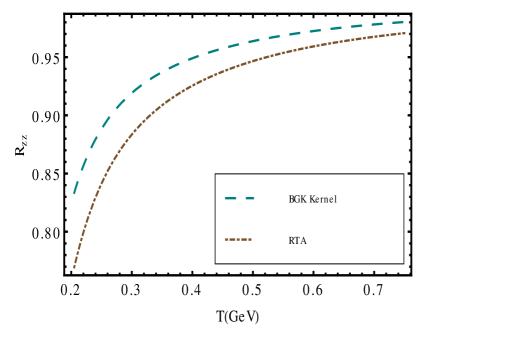
(a)

Figure 1: Temperature behaviour of the ratio $R_{zz}$ at $\mid q_{f}B\mid=10m^{2}_{\pi}$ for RTA and BGK collision kernels considering upto 20 LLs.

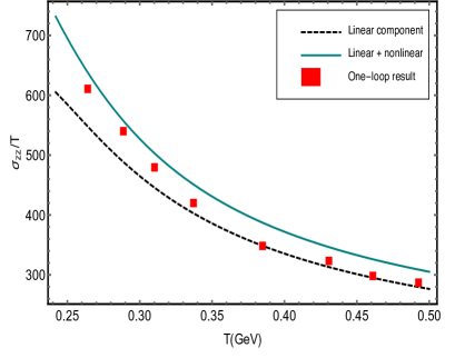
(a)

Figure 2: Behaviour of $\sigma_{zz}/T$ in the LLL approximation of quarks/antiquarks as a function of temperature at $\mid q_{f}B\mid=10m^{2}_{\pi}$ within the RTA. One-loop LLL result for the linear component has been taken from Hattori:2016cnt for the same value of the magnetic field.

III Results and discussions

We initiate our discussion with the temperature behaviour of the longitudinal current density of the hot magnetized QGP in the inhomogeneous electric field. We have estimated the longitudinal current density for both RTA and BGK collision kernels in the presence of the magnetic field considering the HLL contributions. The temperature behaviour of the ratio of the linear component of longitudinal current density to the total longitudinal current density, $R_{zz}$ as described in the Eq. (53) is depicted in the Fig. 1. The ratio $R_{zz}$ is plotted for both RTA and BGK collision terms and we observe a similar behaviour for both the collision integrals. The $R_{zz}$ increase with increasing temperature and seen to saturate at higher temperatures. The temperature behaviour of the ratio $R_{zz}$ in the presence of the magnetic field indicates that the effects of spacetime inhomogeneity of electric field are significant in the temperature regime near to the transition temperature $T_{c}$ whereas the effects are negligible at high temperatures.

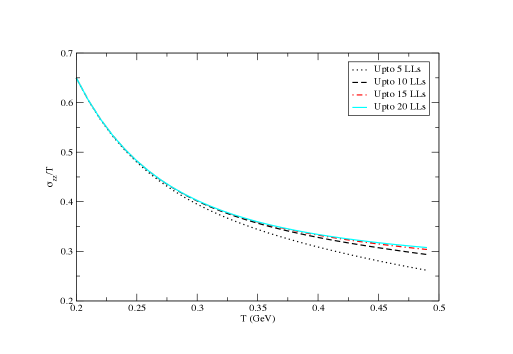
(a)

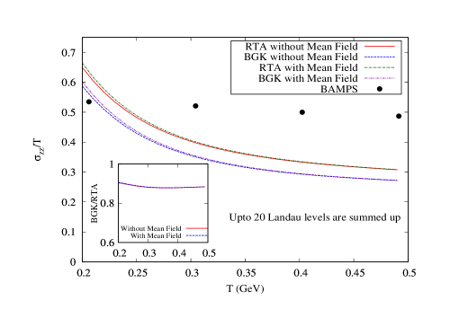
(b)

Figure 3: (Left panel) The effect of HLLs on the temperature behaviour of $\sigma_{zz}/T$ at $\mid q_{f}B\mid=10m^{2}_{\pi}$. (Right panel) Mean field corrections to the $\sigma_{zz}/T$ with the RTA and BGK collision integrals considering up to 20 LLs. The results are also compared with the BAMPS estimation at $B=0$ Greif:2014oia .

The hot medium effects are embedded in the quark and gluonic effective fugacity quasiparton distribution functions as well as in the modified part of dispersion relation. The mean field term of the effective covariant kinetic theory employed in the current analysis involves the fugacity parameters and it’s derivatives. The mean field force terms $F^{i}=\partial_{\mu}(\delta\omega u^{\mu}u^{i})$ are of the second order in gradient since $\delta\omega$ itself is a temperature gradient of the effective fugacity ($z_{g/q}$). Note that at high temperature regime, the effective fugacity varies very slowly with temperature and hence the mean field effects are negligible in that regime.

In the LLL approximation, we have $T^{2}\ll\mid q_{f}B\mid$. In this case, the linear component of the current density in the RTA reduced to the form as defined in Eq. (II.1). The first term in the Eq. (II.1) exactly gives back the leading order contribution of longitudinal current density for $1\rightarrow 2$ processes in the strong magnetic field as estimated in the Refs. Kurian:2017yxj ; Hattori:2016lqx , whereas the second term describes the mean field contribution to the linear component of the current density. In the similar way, the Eq. (II.1) describes the additional component of the current density due to the spacetime inhomogeneity of the field of the magnetized QGP. We compared these results with another approach for the calculation of leading order longitudinal conductivity from one-loop quantum field theory in Fig.2. We observe that $\sigma_{zz}/T$ decrease with increasing temperature. The authors of the Ref. Hattori:2016cnt provide the one-loop result of the linear component of longitudinal conductivity in the strong magnetic field arising from $1\rightarrow 2$ processes of which kinematics are satisfied by fermion dispersion relation with ideal EoS. The quantitative difference in the temperature behaviour of the linear component of longitudinal conductivity around the regime closer to the transition temperature $T_{c}$ reveals the effect of hot QCD medium interactions. The effects of the inhomogeneity of the electric field to the longitudinal conductivity of magnetized QGP are also visible near $T_{c}$. The LLL results in Eq. (II.1) and Eq. (II.1) have an enhancement on the limit $m\rightarrow 0$ as described in Hattori:2016lqx ; Hattori:2016cnt .

In the weakly coupled regime $gT\ll\sqrt{\mid q_{f}B\mid}$, the HLL contributions have significant effect in the transport coefficients Kurian:2018qwb ; Fukushima:2017lvb . The temperature behaviour of $\sigma_{zz}/T$ with HLL contributions are depicted in the Fig. 3 (left panel). Quantitatively, the $\sigma_{zz}/T$ with the HLL effects remains in the range of lattice data results $0.1\leq\sigma/T\leq 1.0$. This observation is quantitatively consistent with the result of the longitudinal conductivity with HLL contribution, $\sigma_{zz}/T\approx 0.7$ at $T=200$ MeV where $\mid q_{f}B\mid=10m^{2}_{\pi}$ and baryon chemical potential $\mu=0$, as described in the recent work Fukushima:2017lvb . The mean field effect induces visible modifications to the longitudinal current density of the hot magnetized QCD matter at the low temperature regimes as plotted in Fig. 3 (right panel). It is to be observed that for the temperatures above $300$MeV, the mean field induced corrections are extremely mild. Their inclusion is essential to describe the behaviour of the current density in the temperatures closer to the transition temperature $T_{c}$. We observe similar temperature behaviour of $\sigma_{zz}/T$ for both RTA and BGK collision kernel. The quantitative difference in the results with RTA and BGK are depicted in Fig. 3 (right panel). We have also compared the HLL result for $\sigma_{zz}/T$ with the BAMPS estimation at $B=0$ Greif:2014oia .

Finally, we have observed that the effects of inhomogeneity of the electric field on $\sigma_{zz}$ are significant in the lower temperature regimes. The EoS dependence of the longitudinal conductivity is more visible near to the transition temperature. Also, note that the HLL contributions to the conductivity are significant in the weakly coupled regime.

IV Conclusion and Outlook

In conclusion, we have obtained the temperature behaviour of the longitudinal current density and the conductivity of the hot interacting QCD matter in the presence of the magnetic field. We considered the effects of spacetime inhomogeneity of the electric field and the contribution of higher Landau levels in the analysis. We have incorporated the hot QCD medium interactions by exploiting the quasiparticle description of quark and gluonic degrees of freedom. We have estimated the longitudinal conductivity for both RTA and BGK collision term in the magnetized QGP medium. Setting up a $(1+1)-$dimensional effective covariant kinetic theory with proper collision integral defines the mean field force term which indeed appears as the mean field corrections to the longitudinal current density and conductivity. The mean field contributions appeared to be significant in the vicinity of the transition temperature $T_{c}$. The above observation is in line with the earlier results for transport coefficients Kurian:2018qwb . We employed RTA for the computation of the longitudinal current density for the $1\rightarrow 2$ processes which are dominant in the presence of the magnetic field. Furthermore, the current density and conductivity with the BGK collision kernel have been computed in the magnetic field followed by the comparison of the results with that of RTA.

The effects of inhomogeneity of the electric field to the longitudinal current density and the conductivity are seen to be quite significant at the temperature regime near to the transition temperature $T_{c}$. The ratio $R_{zz}$ varies between $75\%-95\%$ in the temperature range $200$ MeV$-750$ MeV for both RTA and BGK collision kernels. Notably, in the weakly coupled regime $gT\ll\sqrt{\mid q_{f}B\mid}$, the inclusion of higher Landau level contribution is essential in the estimation of longitudinal conductivity of the magnetized medium. Finally, both the mean field corrections and the effects of electric field inhomogeneity seen to have significant impact on the longitudinal current density and the electrical conductivity in the presence of the strong magnetic field.

We intend to estimate the electromagnetic responses of the chiral plasma with the mean field contribution in the near future. In addition, developing the second order dissipative relativistic hydrodynamics for the magnetized QGP medium from transport theory with the EQPM would be another interesting direction to work.

Appendix A LLL Longitudinal conductivity within RTA at $\mu\neq 0$

The extension of the EQPM to finite baryon/quark chemical potential $\mu$ in the presence of the strong magnetic field is quite straightforward and has the form,

$$f^{0}_{q/\bar{q}}=\dfrac{z_{q}\exp{[-\beta(\sqrt{p_{z}^{2}+m^{2}}\mp\mu)]}}{1+z_{q}\exp{[-\beta(\sqrt{p_{z}^{2}+m^{2}}\mp\mu)]}}.$$ (55)

Here, $z_{g}$, $z_{q}$ are not related with any conserved number current in the hot QCD medium. They have been merely introduced to encode the hot QCD medium effects in the EQPM. Following same prescriptions in the derivation of relaxation time as in the Ref. Kurian:2018dbn , $\tau_{eff}$ for the $1\rightarrow 2$ processes with finite chemical potential $\mu$ can be expressed as,

$$\tau^{-1}_{eff}=\dfrac{2\alpha_{eff}}{\omega_{p}(1-f^{(0)}_{q})}\dfrac{z_{q}}{(\exp{(\dfrac{\mu}{T})}+z_{q})}(1+f^{(0)}_{g}(E_{p}))\ln(T/m),$$ (56)

in which $\alpha_{eff}(T,\mu,\mid q_{f}B\mid)$ is the effective coupling with finite chemical potential and has the following form Kurian:2018qwb ,

$$\dfrac{\alpha_{eff}}{\alpha_{s}(T)}=\dfrac{\dfrac{6T^{2}}{\pi^{2}}PolyLog[2,z_{g}]+\dfrac{3\mid q_{f}B\mid}{\pi^{2}}\Bigg{(}\dfrac{z_{q}}{(1+z_{q})}+\dfrac{\mu^{2}}{2T^{2}}\dfrac{(z_{q}-z^{2}_{q})}{(1+z_{q})^{3}}\Bigg{)}}{T^{2}+\dfrac{3\mid q_{f}B\mid}{2\pi^{2}}}.$$ (57)

Solving Eq. (19) with finite chemical potential, we have,

$${J_{z}}_{(l)} =-\dfrac{q_{f}^{2}}{2\pi}\dfrac{\mid q_{f}B\mid}{(2\pi)}\dfrac{T}{\ln(T/m)}h_{(l)}E, {J_{z}}_{(nl)}=\dfrac{q_{f}^{2}}{2\pi}\dfrac{\mid q_{f}B\mid}{(2\pi)}\dfrac{T^{2}}{48(\ln(T/m))^{2}}h_{(nl)}(\dot{E}+\partial_{z}E),$$ and (58)

where the $h_{(l)}(z_{g},z_{q},\mu/T)$ and $h_{(nl)}(z_{g},z_{q},\mu/T)$ describe the hot medium interactions and have the form,

$$h_{(l)} =\dfrac{(1+z_{q}e^{-\mu/T})}{\alpha_{eff}}\Bigg{\{}\Big{[}(-z_{g}-z_{q}e^{\mu/T})\Big{]}+\Big{[}(-z_{g}+z_{q}e^{\mu/T})\bigg{(}\ln(1+\dfrac{e^{-\mu/T}}{z_{q}})-\ln(1+z_{q}e^{\mu/T})\bigg{)}\Big{]}$$

$$-\Big{[}e^{2\mu/T}\bigg{(}z_{g}+z_{q}e^{-\mu/T}-(-z_{g}+z_{q}e^{-\mu/T})\Big{(}\ln(1+\dfrac{e^{\mu/T}}{z_{q}})-\ln(1+z_{q}e^{-\mu/T})\Big{)}\bigg{)}\Big{]}\Bigg{\}}\dfrac{1}{8z_{q}^{2}m^{2}},$$ (60)

and

$$h_{(nl)} =\Bigg{[}\Bigg{\{}e^{-4\mu/T}(z_{q}+e^{\mu/T})^{2}\Big{[}(z_{q}+z_{g}e^{\mu/T})\bigg{(}z_{q}+z_{g}e^{\mu/T}+3(z_{g}e^{\mu/T}-z_{q})\ln(1+\dfrac{e^{\mu/T}}{z_{q}})+(3z_{q}-3z_{g}e^{\mu/T})$$

$$\times\ln(1+z_{q}e^{-\mu/T})\bigg{)}-2(z^{2}_{q}+z^{2}_{g}e^{2\mu/T}-z_{q}z_{g}e^{\mu/T})\Big{(}PolyLog[2,-\dfrac{e^{\mu/T}}{z_{q}}]+PolyLog[2,-z_{q}e^{-\mu/T}]\Big{)}\Big{]}\Bigg{\}}$$

$$+\Bigg{\{}(1+z_{q}e^{\mu/T})^{2}\Big{[}(z_{g}+z_{q}e^{\mu/T})\bigg{(}z_{g}+z_{q}e^{\mu/T}+3(z_{g}-z_{q}e^{\mu/T})\ln(1+z_{q}^{-1}e^{-\mu/T})\bigg{)}+3(z_{g}-z_{q}e^{\mu/T})$$

$$\times\ln(1+z_{q}e^{\mu/T})-2(z^{2}_{q}e^{2\mu/T}+z^{2}_{g}-z_{q}z_{g}e^{\mu/T})\Big{(}PolyLog[2,-\dfrac{e^{-\mu/T}}{z_{q}}]+PolyLog[2,-z_{q}e^{\mu/T}]\Big{)}\Big{]}\Bigg{\}}\Bigg{]}\dfrac{(z_{q}+e^{\mu/T})^{2}}{\alpha^{2}_{eff}z_{q}^{6}m^{4}}.$$ (61)

References

- (1) Adams et al. (STAR Collaboration), Nucl. Phys. A757, 102 (2005); K. Adcox et al. (PHENIX Collaboration), Nucl. Phys. A757, 184 (2005); B.B. Back et al. (PHOBOS Collaboration), Nucl. Phys. A757, 28 (2005); A. Arsence et al. (BRAHMS Collaboration), Nucl. Phys. A757, 1 (2005).
- (2) K. Aamodt et al. [ALICE Collaboration], Phys. Rev. Lett. 105, 252301 (2010).
- (3) V. Skokov, A. Y. Illarionov and V. Toneev, Int. J. Mod. Phys. A 24, 5925 (2009).
- (4) W.-T. Deng, and Xu-Guang Huang, Phys. C 85, 044907 (2012).
- (5) Y. Zhong, C. B. Yang, X. Cai and S. Q. Feng, Adv. High Energy Phys. 2014 (2014) 193039.
- (6) S. K. Das, S. Plumari, S. Chatterjee, J. Alam, F. Scardina and V. Greco, Phys. Lett. B 768, 260 (2017).
- (7) S. Ghosh and V. Chandra, Phys. Rev. D 98, no. 7, 076006 (2018).
- (8) A. Mukherjee, S. Ghosh, M. Mandal, P. Roy and S. Sarkar, Phys. Rev. D 96, no. 1, 016024 (2017).
- (9) B. Karmakar, A. Bandyopadhyay, N. Haque and M. G. Mustafa, arXiv:1804.11336 [hep-ph].
- (10) A. Das, A. Bandyopadhyay, P. K. Roy and M. G. Mustafa, Phys. Rev. D 97, no. 3, 034024 (2018).
- (11) B. Karmakar, R. Ghosh, A. Bandyopadhyay, N. Haque and M. G. Mustafa, arXiv:1902.02607 [hep-ph](2019).
- (12) A. Bandyopadhyay, B. Karmakar, N. Haque and M. G. Mustafa, arXiv:1702.02875 [hep-ph].
- (13) S. Koothottil and V. M. Bannur, arXiv:1811.05377 [nucl-th].
- (14) V. Roy, S. Pu, L. Rezzolla and D. H. Rischke, Phys. Rev. C 96, no. 5, 054909 (2017).
- (15) G. Coci, L. Oliva, S. Plumari, S. K. Das and V. Greco, Nucl. Phys. A 982, 189 (2019).
- (16) K. Fukushima, D. E. Kharzeev and H. J. Warringa, Phys. Rev. D 78, 074033 (2008), D. E. Kharzeev, L. D. McLerran, H. J. Warringa, Nucl. Phys. A803, 227 (2008),D. E. Kharzeev, Annals Phys. 325, 205 (2010), D. E. Kharzeev and D. T. Son, Phys. Rev. Lett. 106, 062301 (2011).
- (17) A. V. Sadofyev and M. V. Isachenkov, Phys. Lett. B 697, 404 (2011), A. V. Sadofyev, V. I. Shevchenko and V. I. Zakharov, Phys. Rev. D 83, 105025 (2011).
- (18) X. G. Huang, Y. Yin, and J. Liao Nucl. Phys. A956, 661 (2016).
- (19) D. She, S. Q. Feng, Y. Zhong and Z. B. Yin, Eur. Phys. J. A 54, no. 3, 48 (2018).
- (20) X. G. Huang, Y. Yin and J. Liao, Nucl. Phys. A 956, 661 (2016) doi:10.1016/j.nuclphysa.2016.01.064 [arXiv:1512.06602 [nucl-th]].
- (21) D. E. Kharzeev, J. Liao, S. A. Voloshin and G. Wang, Prog. Part. Nucl. Phys. 88, 1 (2016).
- (22) A. Avkhadiev and A. V. Sadofyev, Phys. Rev. D 96, no. 4, 045015 (2017).
- (23) N. Yamamoto, Phys. Rev. D 96, no. 5, 051902 (2017).
- (24) L. Adamczyk et al. [STAR Collaboration], Nature 548, 62 (2017).
- (25) F. Becattini, I. Karpenko, M. Lisa, I. Upsal and S. Voloshin, Phys. Rev. C 95, no. 5, 054902 (2017).
- (26) K. Hattori, X. G. Huang, D. H. Rischke and D. Satow, Phys. Rev. D 96, no. 9, 094009 (2017).
- (27) K. Hattori, S. Li, D. Satow and H. U. Yee, Phys. Rev. D 95, no. 7, 076008 (2017).
- (28) M. Kurian, S. Mitra, S. Ghosh and V. Chandra, Eur. Phys. J. C 79, no. 2, 134 (2019) [arXiv:1805.07313 [nucl-th]].
- (29) M. Kurian and V. Chandra, Phys. Rev. D 96, no. 11, 114026 (2017).
- (30) K. Hattori and D. Satow, Phys. Rev. D 94, no. 11, 114032 (2016).
- (31) K. Fukushima and Y. Hidaka, Phys. Rev. Lett. 120, no. 16, 162301 (2018).
- (32) M. Kurian and V. Chandra, Phys. Rev. D 97, no. 11, 116008 (2018).
- (33) S. Rath and B. K. Patra, arXiv:1901.03855 [hep-ph].
- (34) W. Li, S. Lin and J. Mei, Phys. Rev. D 98, no. 11, 114014 (2018).
- (35) B. Feng, Phys. Rev. D 96, no. 3, 036009 (2017).
- (36) P. Mohanty, A. Dash and V. Roy, arXiv:1804.01788 [nucl-th].
- (37) X. G. Huang, A. Sedrakian and D. H. Rischke, Annals Phys. 326, 3075 (2011).
- (38) R. Critelli, S. I. Finazzo, M. Zaniboni and J. Noronha, Phys. Rev. D 90, no. 6, 066006 (2014).
- (39) K. Tuchin, Phys. Rev. C 88, no. 2, 024911 (2013).
- (40) M. Hongo, Y. Hirono and T. Hirano, Phys. Lett. B 775, 266 (2017).
- (41) K. Tuchin, Phys. Rev. C 87, no. 2, 024912 (2013).
- (42) B. G. Zakharov, arXiv:1708.05882 [nucl-th].
- (43) K. Tuchin, Adv. High Energy Phys. 2013, 490495 (2013).
- (44) D. Satow, Phys. Rev. D 90, no. 3, 034018 (2014).
- (45) V. Chandra and V. Ravishankar, Phys. Rev. D 84, 074013 (2011).
- (46) S. Mitra and V. Chandra, Phys. Rev. D 97, no. 3, 034032 (2018).
- (47) V. Chandra, R. Kumar and V. Ravishankar, Phys. Rev. C 76, 054909 (2007).
- (48) S. Mitra and V. Chandra, Phys. Rev. D 96, no. 9, 094003 (2017).
- (49) M. Cheng et al., Phys. Rev. D 77, 014511 (2008).
- (50) S. Borsanyi, Z. Fodor, C. Hoelbling, S. D. Katz, S. Krieg, Kalman K. Szabo, Phys. Lett. B 370, 99-104 (2014).
- (51) S. Li and H. U. Yee, Phys. Rev. D 97, no. 5, 056024 (2018).
- (52) F. Bruckmann, G. Endrodi, M. Giordano, S. D. Katz, T. G. Kovacs, F. Pittler and J. Wellnhofer, Phys. Rev. D 96, no. 7, 074506 (2017).
- (53) A. N. Tawfik, J. Phys. Conf. Ser. 668, no. 1, 012082 (2016).
- (54) V. P. Gusynin, V. A. Miransky and I. A. Shovkovy, Nucl. Phys. B 462, 249 (1996).
- (55) S. Mitra and V. Chandra, Phys. Rev. D 94, no. 3, 034025 (2016).
- (56) P. L. Bhatnagar, E. P. Gross, and M. Krook, Phys. Rev. 94, 511 (1954).
- (57) Bjoern Schenke, Michael Strickland, Carsten Greiner, Markus H. Thoma, Phys. Rev. D 73, 125004 (2006).
- (58) Bing-feng Jiang, De-fu Hou and Jia-rong Li, Phys. Rev. D 94, 074026 (2016).
- (59) M. Carrington, T. Fugleberg, D. Pickering, and M. Thoma, Can. J. Phys. 82, 671 (2004).
- (60) A. Kumar, M. Y. Jamal, V. Chandra and J. R. Bhatt, Phys. Rev. D 97, no. 3, 034007 (2018).
- (61) M. Greif, I. Bouras, C. Greiner and Z. Xu, Phys. Rev. D 90, no. 9, 094014 (2014).