Batch Virtual Adversarial Training for Graph Convolutional Networks

Abstract

We present batch virtual adversarial training (BVAT), a novel regularization method for graph convolutional networks (GCNs). BVAT addresses the shortcoming of GCNs that do not consider the smoothness of the model’s output distribution against local perturbations around the input. We propose two algorithms, sample-based BVAT and optimization-based BVAT, which are suitable to promote the smoothness of GCN classifiers by generating virtual adversarial perturbations for either a subset of nodes far from each other or all nodes with an optimization process. Extensive experiments on three citation network datasets Cora, Citeseer and Pubmed and a knowledge graph dataset Nell validate the effectiveness of the proposed method, which establishes state-of-the-art results in the semi-supervised node classification task.

1 Introduction

Recent neural network models for graph-structured data (Kipf & Welling, 2017; Hamilton et al., 2017; Veličković et al., 2018) demonstrate remarkable performance in the semi-supervised node classification task. These methods essentially adopt different aggregators to aggregate feature information from the neighborhood of a node to obtain node prediction. The aggregators promote the smoothness between nodes in a neighborhood, which is helpful for semi-supervised node classification based on the assumption that connected nodes in the graph are likely to have similar representations (Kipf & Welling, 2017). However, these methods only consider the smoothness between nodes in a neighborhood without considering the smoothness of the output distribution of the node classifier. Previous works have confirmed that smoothing the output distribution of a classifier (i.e., encouraging the classifier to produce similar outputs) against local perturbations around the input can improve its generalization performance in supervised and especially semi-supervised learning (Wager et al., 2013; Sajjadi et al., 2016; Laine & Aila, 2017; Miyato et al., 2018; Luo et al., 2018). Moreover, it’s crucial to encourage the smoothness of the output distribution of aggregator-based graph models since the receptive field (e.g., Fig. 1a) of a single node grows exponentially with respect to the number of aggregators in the model (Chen & Zhu, 2017), and neural network models tend to be non-smooth with such high dimensional input space (Goodfellow et al., 2015; Peck et al., 2017). Therefore, it is necessary to encourage the smoothness of the output distribution of existing graph models.

Figure 1: (a) The receptive field (marked by red) of a node $u$ in two-layer GCNs. (b) In S-BVAT, two nodes $u$ and $v$ are selected to calculate the LDS loss, and the virtual adversarial perturbations are applied to the features in their receptive fields (marked by red and blue), which do not have intersection. (c) In O-BVAT, all nodes are included to calculate the LDS loss and the virtual adversarial perturbations for all nodes are optimized together.

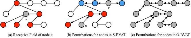
Virtual adversarial training (VAT) (Miyato et al., 2018, 2017) is an effective regularization method to encourage the smoothness of the output distribution of the classifier. However, the straightforward extension of VAT to graph-based classification models is less effective. The reason is that graph-based classifiers predict a node $u$ based on the features of all nodes in its receptive field (i.e., $RF_{u}$), as shown in Fig. 1a, and consequently, the gradient of $u$’s loss can be back propagated to all nodes in $RF_{u}$. It means that the virtual adversarial perturbation calculated for node $u$ will modify the features of every node in $RF_{u}$. Thus, when applying VAT into graph models and training with batch gradient descent (Kipf & Welling, 2017) or stochastic gradient descent (Hamilton et al., 2017; Chen & Zhu, 2017), once the batch (or mini-batch) contains other nodes whose receptive fields include $u$, the virtual adversarial perturbations generated for $u$ and those nodes overlap. As a result, the overall perturbation for node $u$ is actually not the worst-case virtual adversarial perturbation, making VAT inefficient to encourage the smoothness of the model’s output distribution and unable to push decision boundaries of the model away from real data instances effectively.

Given the aforementioned issue, we aim to generate virtual adversarial perturbations perceiving the connectivity patterns between nodes in the graph to promote the smoothness of the node classifier’s output distribution. In this paper, we propose batch virtual adversarial training (BVAT) algorithms. Specifically, we focus on the typical and effective graph convolutional networks (GCNs) (Kipf & Welling, 2017), and propose a sample-based BVAT algorithm (S-BVAT) to craft local virtual adversarial perturbations for a subset of separable nodes and an optimization-based BVAT algorithm (O-BVAT) that generates adversarial perturbations at all nodes. BVAT exploits the high efficiency of batch gradient descent in GCNs. To validate the effectiveness of BVAT, we conduct experiments on four challenging node classification benchmarks: Cora, Citeseer, Pubmed citation datasets as well as a knowledge graph dataset Nell. BVAT establishes state-of-the-art results across all datasets with a tolerable additional computation complexity.

2 Related Work

Learning node representations based on graph for semi-supervised learning and unsupervised learning has drawn increasing attention and has been developed mainly toward two directions: spectral approaches (Zhu et al., 2003; Belkin et al., 2006; Weston et al., 2012; Defferrard et al., 2016; Kipf & Welling, 2017) and non-spectral approaches (Perozzi et al., 2014; Tang et al., 2015; Grover & Leskovec, 2016; Yang et al., 2016; Monti et al., 2017; Hamilton et al., 2017; Veličković et al., 2018). There is also an interest in applying regularization terms (Miyato et al., 2018; Laine & Aila, 2017; Tarvainen & Valpola, 2017; Luo et al., 2018) to semi-supervised learning based on the cluster assumption (Chapelle & Zien, 2005). Among them, virtual adversarial training (VAT) has been proved successful in various domains (Miyato et al., 2017, 2018). However, VAT is not effective enough when straightforwardly applied to the models that deal with graph-structured data because of the interrelationship between different nodes, as stated in Sec. 1. Thus we propose a novel regularization BVAT to address this issue. The works of adversarial attacks on graph-structure data (Zügner et al., 2018; Dai et al., 2018) also share the idea of considering the connectivity patterns of the graph to generate adversarial perturbations, but our work focuses more on semi-supervised node classification instead of performing adversarial attacks. Moreover, graph partition neural networks proposed by (Liao et al., 2018) has the similar idea of splitting original graph into disjoint subgraphs to S-BVAT, but it is dedicated to promoting the efficiency of information propagation in graph rather than the smoothness of the output distribution.

3 Batch Virtual Adversarial Training

In this section, we first extend virtual adversarial training (VAT) (Miyato et al., 2018) to graph convolutional networks (GCNs) and discuss its shortcomings. We then propose the batch virtual adversarial training (BVAT) algorithms which are more suitable for GCNs.

3.1 Virtual Adversarial Training for Graph Convolutional Networks

Virtual adversarial training (VAT) (Miyato et al., 2018) encourages the smoothness by training the model to be robust against local worst-case virtual adversarial perturbation. In VAT, the local distributional smoothness (LDS) is defined by a virtual adversarial loss as

$$\mathrm{LDS}(x,\mathcal{W},r_{\mathrm{vadv}})=D_{\mathrm{KL}}\big{(}p(y|x,\hat{\mathcal{W}})||p(y|x+r_{\mathrm{vadv}},\mathcal{W})\big{)},$$ (1)

where $p(y|x,\mathcal{W})$ is the prediction distribution parameterized by $\mathcal{W}$ (i.e., trainable parameters), $D_{\mathrm{KL}}(\cdot,\cdot)$ is the KL divergence of two distributions, $\hat{\mathcal{W}}$ denotes the current estimation of the parameters $\mathcal{W}$ and $r_{\mathrm{vadv}}$ is the virtual adversarial perturbation found by

$$\begin{split}r_{\mathrm{vadv}}&=\mathop{\arg\max}\limits_{r;||r||_{2}\leq\epsilon}\mathrm{LDS}(x,\mathcal{W},r)\\ &=\mathop{\arg\max}\limits_{r;||r||_{2}\leq\epsilon}D_{\mathrm{KL}}\big{(}p(y|x,\hat{\mathcal{W}})||p(y|x+r,\mathcal{W})\big{)}.\end{split}$$ (2)

A straightforward extension into GCNs is using the average LDS loss for all nodes as a regularization term

$$\mathcal{R}_{\mathrm{vadv}}(\mathcal{V},\mathcal{W})=\frac{1}{N}\sum\limits_{u\in\mathcal{V}}\mathrm{LDS}(X_{u},\mathcal{W},r_{\mathrm{vadv},u}),$$ (3)

where $\mathcal{V}$ denotes the node set of the graph containing $N$ elements and $X_{u}$ is the input feature matrix of all nodes in $RF_{u}$. $r_{\mathrm{vadv},u}$ is the virtual adversarial perturbation matrix for node $u$ in the same size as $X_{u}$ and is approximated by the first dominant eigenvector of the Hessian matrix of $\mathrm{LDS}(X_{u},\mathcal{W},r)$ using a power iteration method with $T$ iterations (Miyato et al., 2018). The overall loss is

$$\begin{split}\mathcal{L}=\mathcal{L}_{0}+\alpha\cdot\frac{1}{|\mathcal{V}|}\sum\limits_{u\in\mathcal{V}}E\big{(}p(y|X_{u},\mathcal{W})\big{)}+\beta\cdot\mathcal{R}_{\mathrm{vadv}}(\mathcal{V},\mathcal{W}),\end{split}$$ (4)

where $\mathcal{L}_{0}$ is the average cross-entropy loss of all labeled nodes and $E(\cdot)$ is the conditional entropy of a distribution, which is widely used in the semi-supervised classification task (Grandvalet & Bengio, 2005) to encourage one-hot predictions. $\alpha$ and $\beta$ are coefficients for conditional entropy and local distributional smoothness.

Notably, the interaction of nodes in the graph reduces the effectiveness of loss $\mathrm{LDS}(X_{u},\mathcal{W},r_{\mathrm{vadv},u})$ since in the batch training, the calculated $r_{\mathrm{vadv},u}$ is the accumulation of the virtual adversarial perturbations generated for all nodes in $RF_{u}$. Therefore, $\|r_{\mathrm{vadv},u}\|_{2}\leq\epsilon$ in Eq. (2) cannot be guaranteed and the resultant perturbations are not the worst-case virtual adversarial perturbations.

3.2 Batch Virtual Adversarial Training

BVAT can perceive the connectivity patterns between nodes and alleviate the interaction effect of virtual adversarial perturbations crafted for all nodes by either stochastically sampling a subset of nodes far from each other or adopting a more powerful optimization process for generating virtual adversarial perturbations. These two approaches are both harmonious with the batch gradient descent optimization method used by GCNs and only increase tolerable additional computation complexity, as shown in Appendix D.

S-BVAT. The motivation of sample-based BVAT is that we expect to make the model be aware of the relationship between nodes and limit the propagation of adversarial perturbations to prevent perturbations from different nodes interacting with each other. In S-BVAT, we generate virtual adversarial perturbations for a subset $\mathcal{V_{S}}\subset\mathcal{V}$ of nodes, whose receptive fields do not overlap with each other. Taking a $K$-layer GCN model for example, the receptive field $RF_{u}$ of a node $u$ contains all the $k$-hop neighbors of it where $0\leq k\leq K$. If we expect $RF_{u}$ doesn’t have intersection with $RF_{v}$, the number of nodes in the shortest path between $u$ and $v$ (denoted as the distance $D_{uv}$) should be at least $2K$ (shown in Fig. 1b). Therefore, we randomly sample a subset $\mathcal{V_{S}}$ of nodes with a fixed size $B$ (e.g., 100) as

$$\mathcal{V_{S}}=\{u|u\in\mathcal{V}\},\;\;\text{s.t.}\;|\mathcal{V_{S}}|=B,\;\forall u,v\in\mathcal{V_{S}},D_{uv}\geq 2K.$$

In this way, the generated perturbations for nodes in $\mathcal{V_{S}}$ do not interact with each other. The regularization term for training is the average LDS loss over nodes in $\mathcal{V_{S}}$ as

$$\mathcal{R}_{\mathrm{vadv}}(\mathcal{V_{S}},\mathcal{W})=\frac{1}{B}\sum\limits_{u\in\mathcal{V_{S}}}LDS(X_{u},\mathcal{W},r_{\mathrm{vadv},u}).$$ (5)

$\mathcal{R}_{\mathrm{vadv}}(\mathcal{V_{S}},\mathcal{W})$ can be seen as an approximate estimation of $\mathcal{R}_{\mathrm{vadv}}(\mathcal{V},\mathcal{W})$. The virtual adversarial perturbations for all nodes in $\mathcal{V_{S}}$ can be processed at the same time in the batch gradient descent. As suggested by (Miyato et al., 2018) and our experiments, one-step power iteration is sufficient for approximating $r_{\mathrm{vadv},u}$ and obtaining high performance. We summarize S-BVAT in Algorithm 1 in Appendix.

O-BVAT. In an alternative way, we propose to generate virtual adversarial perturbations for all nodes in $\mathcal{V}$ by an optimization process, which proves to be more powerful in adversarial attacks than one-step gradient-based methods (Carlini & Wagner, 2017). We maximize the average LDS loss with respect to the whole perturbation matrix $R$ corresponding to the whole feature matrix $X$ so that the neighborhood perturbations $R_{u}$ (i.e., $r_{\mathrm{vadv},u}$) of every node $u$ are adversarial enough. At the same time, we punish the norm of $R$ so that the perturbations are small enough.

Specifically, $R$ is optimized by solving

$$\mathop{\max}\limits_{R}\frac{1}{N}\sum\limits_{u\in\mathcal{V}}D_{\mathrm{KL}}\big{(}p(y|X_{u},\hat{\mathcal{W}})||p(y|X_{u}+R_{u},\mathcal{W})\big{)}\\ -\gamma\cdot\|R\|_{F}^{2},$$ (6)

where $\|R\|_{F}$ is the Frobenius norm of $R$ which makes the optimal perturbation have a small norm, and $\gamma$ is a hyper-parameter to balance the loss terms. We optimize $R$ with an Adam (Kingma & Ba, 2014) optimizer for $T$ iterations. The regularization term in O-BVAT is then the average LDS loss over all nodes in $\mathcal{V}$, similar to Eq. (3). We summarize O-BVAT in Algorithm 2 in Appendix.

4 Experiments

We empirically evaluate the BVAT algorithms through experiments on different datasets. Owing to promoting the smoothness of the model’s output distribution, the BVAT algorithms boost the performance of GCNs significantly and achieve superior results on four popular benchmarks against a wide variety of state-of-the-art methods, which is detailed in Sec. 4.2. We implement BVAT based on the official implementation of GCNs and the experimental setup is detailed in Appendix B.

(a)

(b)

(c)

Figure 2: (a) Comparisons of $\mathcal{R}_{\mathrm{vadv}}$ of VAT, S-BVAT and O-BVAT on a baseline GCN model. (b) Comparisons of $\mathcal{R}_{\mathrm{vadv}}$ of S-BVAT on models trained with and without S-BVAT. (c) Comparisons of $\mathcal{R}_{\mathrm{vadv}}$ of O-BVAT on models trained with and without O-BVAT.

Table 1: Summary of node classification results in terms of test accuracy (%).

Method	Cora	Cireseer	Pubmed	Nell
ManiReg (Belkin et al., 2006)	59.5	60.1	70.7	21.8
SemiEmb (Weston et al., 2012)	59.0	59.6	71.1	26.7
LP (Zhu et al., 2003)	68.0	45.3	63.0	26.5
DeepWalk (Perozzi et al., 2014)	67.2	43.2	65.3	58.1
Planetoid (Yang et al., 2016)	75.7	64.7	77.2	61.9
Monet (Monti et al., 2017)	81.7 $\pm$ 0.5	–	78.8 $\pm$ 0.3	–
GAT (Veličković et al., 2018)	83.0 $\pm$ 0.7	72.5 $\pm$ 0.7	79.0 $\pm$ 0.3	–
GPNN (Liao et al., 2018)	81.8	69.7	79.3	63.9
GCN (Kipf & Welling, 2017)	81.5	70.3	79.0	66.0
GCN w/ random perturbations	82.3 $\pm$ 2.0	71.4 $\pm$ 1.9	79.2 $\pm$ 0.6	65.9 $\pm$ 1.0
GCN w/ VAT	82.8 $\pm$ 0.8	73.0 $\pm$ 0.7	79.5 $\pm$ 0.3	66.0 $\pm$ 1.1
GCN w/ S-BVAT	83.4 $\pm$ 0.6	73.1 $\pm$ 1.3	79.6 $\pm$ 0.5	66.0 $\pm$ 0.9
GCN w/ O-BVAT	83.6 $\pm$ 0.5	74.0 $\pm$ 0.6	79.9 $\pm$ 0.4	67.1 $\pm$ 0.6

4.1 Effectiveness of BVAT

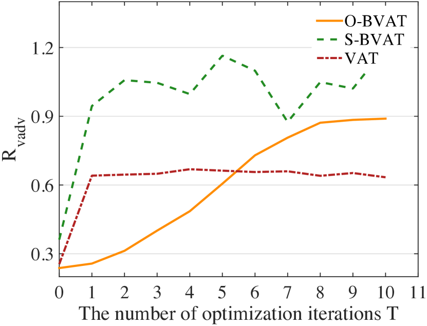
We evaluate the effectiveness of the BVAT algorithms by assessing the virtual adversarial perturbations generated by them for graph data. First, we train a vanilla GCN model on Cora. Then, we use VAT, S-BVAT and O-BVAT to manufacture virtual adversarial perturbations and calculate the regularization term $\mathcal{R}_{\mathrm{vadv}}$ averaged on all the nodes $\mathcal{V}$ (in VAT and O-BVAT) or a subset of nodes $\mathcal{V_{S}}$ (in S-BVAT). $\mathcal{R}_{\mathrm{vadv}}$ indicates whether the perturbations are worst-case locally adversarial or not. We plot $\mathcal{R}_{\mathrm{vadv}}$ in Fig. 2(a).

It is clear that O-BVAT and S-BVAT achieve higher $\mathcal{R}_{\mathrm{vadv}}$ values than VAT, which demonstrates that BVAT can find virtual adversarial perturbations which are more likely to be in the worst-case direction. For both S-BVAT and VAT, We can observe a significant jump of the $\mathcal{R}_{\mathrm{vadv}}$ value when $T$ changes from 0 (random perturbations) to 1, but no much more with larger $T$. Therefore we set $T=1$ in VAT and S-BVAT. However, $\mathcal{R}_{\mathrm{vadv}}$ of O-BVAT increases monotonically with respect to $T$ and converges at about 10 steps, so we set $T=10$ in the following experiments.

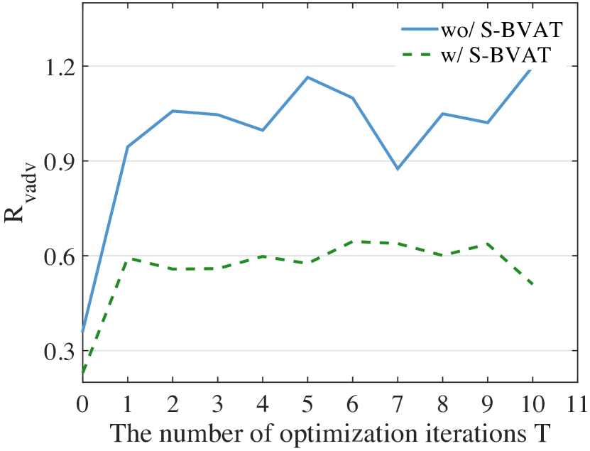
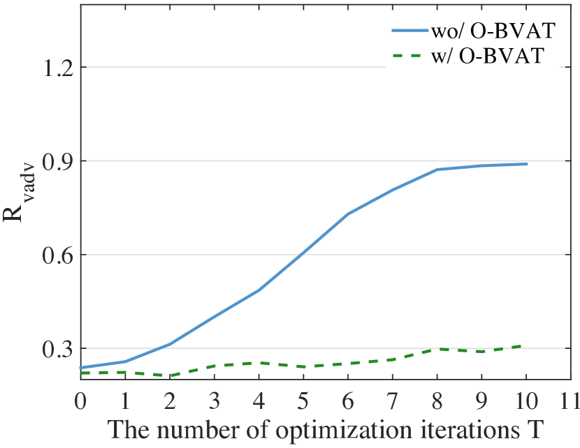
On the other hand, we compare the robustness (i.e., smoothness in the worst-case direction) of the models trained with S-BVAT/O-BVAT with that of the models trained without S-BVAT/O-BVAT by calculating the $\mathcal{R}_{\mathrm{vadv}}$ values. Fig. 2(b) and 2(c) show the results respectively. The models trained with BVAT (S-BVAT or O-BVAT) have lower $\mathcal{R}_{\mathrm{vadv}}$ values than the vanilla GCN models, which indicates that the models trained with BVAT are more robust against the adversarial perturbations and more smooth in the input space.

4.2 Semi-supervised Node Classification

To empirically validate the effectiveness of smoothing output distribution, we deploy BVAT and VAT algorithms for semi-supervised node classification on the Cora, Citeseer, Pubmed and Nell, and compare with state-of-the-art methods in Table 1. We also train a GCN model with random input perturbations as a baseline. We report the averaged results of 10 runs with different random seeds.

The proposed GCNs with VAT, GCNs with S-BVAT and GCNs with O-BVAT all outperform the vanilla GCNs and GCNs trained with random input perturbations by a large margin across all the four datasets. Furthermore, as expected, O-BVAT boosts the performance significantly and establishes state-of-the-art results. O-BVAT uses the LDS loss on all nodes, which may be more efficient than that on a subset of nodes used by S-BVAT.

5 Conclusion

In this paper, we proposed batch virtual adversarial training algorithms, which can smooth the output distribution of graph-based classifiers and are essentially suitable for any aggregator-based graph neural networks. In particular, we presented sample-based batch virtual adversarial training and optimization-based virtual adversarial training algorithms respectively. Experimental results demonstrate the effectiveness of the proposed method on various datasets in the semi-supervised node classification task. BVAT outperforms the current state-of-the-art methods by a large margin.

Appendix A Algorithms for BVAT

We present the detailed algorithms for sample-based batch virtual adversarial training (S-BVAT) and optimization-based batch virtual adversarial training (O-BVAT) in Algorithm 1 and Algorithm 2, respectively.

Algorithm 1 Sample-based batch virtual adversarial training (S-BVAT)

1:  $\mathcal{V_{S}}=\varnothing$, $\mathcal{V_{C}}=\mathcal{V}$.

2:  while $|\mathcal{V_{S}}|<B$ do

3:     Choose a node $u$ from $\mathcal{V_{C}}$ randomly and add $u$ to $\mathcal{V_{S}}$.

4:     Remove all nodes in the $k$-hop ($\forall k\in[0,2K]$) neighborhood of $u$ from $\mathcal{V_{C}}$.

5:     Initialize $r_{\mathrm{vadv},u}$ from an iid Gaussian distribution and normalize it as $\|r_{\mathrm{vadv},u}\|_{F}=1$.

6:  end while

7:  Calculate $r_{\mathrm{vadv},u}$ by taking the gradient of $\mathrm{LDS}(X_{u},\mathcal{W},r)$ with respect to $r$:

$$g_{u}\leftarrow\nabla_{r}D_{\mathrm{KL}}\big{(}p(y|X_{u},\hat{\mathcal{W}})||p(y|X_{u}+r,\mathcal{W})\big{)}|_{r=\xi r_{\mathrm{vadv},u}},$$

$$r_{\mathrm{vadv},u}=\epsilon\cdot g_{u}/\|g_{u}\|_{F}.$$

8:  return $\nabla_{\mathcal{W}}\mathcal{R}_{\mathrm{vadv}}(\mathcal{V_{S}},\mathcal{W})|_{\mathcal{W}=\hat{\mathcal{W}}}.$

Algorithm 2 Optimization-based batch virtual adversarial training (O-BVAT)

1:  Initialize $R^{(0)}\in\mathbb{R}^{N\times D}$ from an iid Gaussian distribution.

2:  for $i$ = 1 to $T$ do

3:     Calculate the gradient of Eq. (6) with respect to $R^{(i-1)}$ as $g^{(i)}$.

4:     Use an Adam optimizer to perform gradient ascent as $R^{(i)}\leftarrow\textrm{Adam}(R^{(i-1)},g^{(i)})$.

5:  end for

6:  $R\leftarrow R^{(T)}$.

7:  return $\nabla_{\mathcal{W}}\mathcal{R}_{\mathrm{vadv}}(\mathcal{V},\mathcal{W})|_{\mathcal{W}=\hat{\mathcal{W}}}$.

Appendix B Experimental Setup

We examine BVAT on the three citation network datasets Cora, Citeseer and Pubmed (Sen et al., 2008) and one knowledge graph dataset Nell (Yang et al., 2016) with the same train/validation/test splits as (Yang et al., 2016) and (Kipf & Welling, 2017). The details of the four datasets are summarized in Table 2. We use the same preprocessing strategies as GCNs. The dimension of the preprocessed node features in Nell is $61,278$, so the input sparse matrix $X\in\mathbb{R}^{65755\times 61278}$ is too large to be converted to a dense matrix that doesn’t exceed the GPU memory (GTX 1080Ti). As a result, BVAT algorithms construct sparse virtual adversarial perturbations $R$ for Nell. We use the same architecture, initialization, dropout rate, $L_{2}$ regularization factor, number of hidden units and number of epochs as GCNs.

Table 2: Statistics of the datasets used in our experiments.

	Cora	Cireseer	Pubmed	Nell
Nodes	2,708	3,327	19,717	65,755
Edges	5,429	4,732	44,338	266,144
Features	1,433	3,703	500	61,278
Classes	7	6	3	105
Label rate	0.052	0.036	0.003	0.001

For S-BVAT, we fix $B=100$, $\xi=10^{-6}$ and $T=1$. We set the perturbation size $\epsilon=0.03$ for Cora and Citeseer and $\epsilon=0.003$ for Pubmed and Nell. For O-BVAT, we run an Adam optimizer with learning rate $0.001$ for $T=10$ iterations. We set $\gamma=0.01$ on Pubmed and $\gamma=1$ on the others. We tune the hyper-parameters $\alpha$ and $\beta$ because the label rate, feature size and number of edges vary significantly across different datasets.

(a)

(b)

Figure 3: (a) Effect of $\epsilon$ on the validation performance of S-BVAT for Cora and Citeseer. (b) Effect of $\alpha$ on the validation performance of S-BVAT and O-BVAT for Cora.

Appendix C Ablation study of $\epsilon$ and $\alpha$

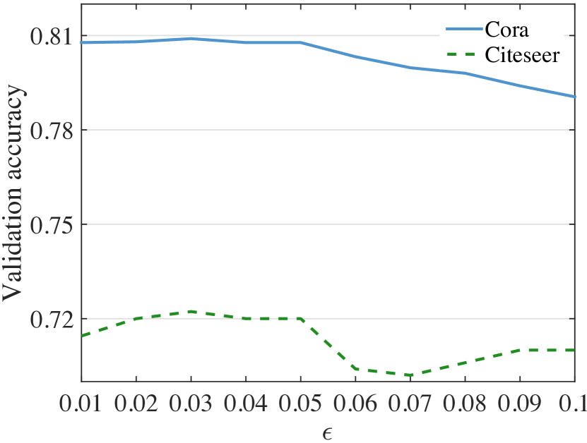
To investigate how the perturbation size $\epsilon$ in S-BVAT affects the final classification results, we conduct an ablation study in Fig. 3(a), where we plot the validation accuracy of the trained models on Cora and Citeseer with respect to the varied $\epsilon$ while keeping the other hyper-parameters fixed (on Cora, we set $\beta=1.2$ and $\alpha=0.7$; on Citeseer, we set $\beta=0.8$ and $\alpha=0.7$). As we have observed, S-BVAT is not sensitive to $\epsilon$ when it changes from 0.01 to 0.1 and we choose $\epsilon=0.03$ for both Cora and Citeseer. The conclusion is also true for Pubmed and Nell, where $\epsilon$ is set to $0.003$ due to the smaller norm of input features in these two datasets.

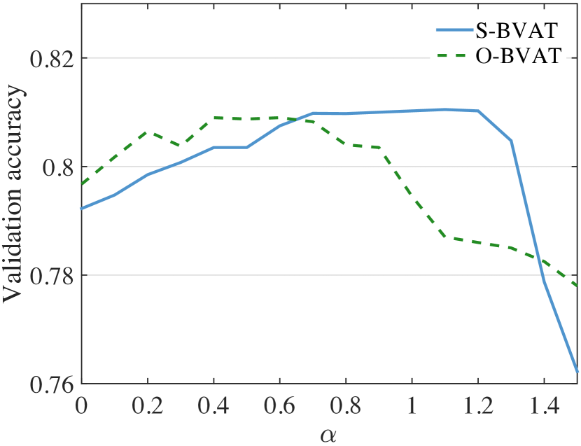
Incorporating the conditional entropy term $E(\cdot)$ into training of semi-supervised tasks is confirmed useful generally (Grandvalet & Bengio, 2005). We expect to determine the importance of the role it plays in the BVAT algorithms. Thus, we conduct two set of experiments on Cora by assessing the validation accuracy of the models trained with different values of $\alpha$ in the range $[0,1.5]$ with a granularity $0.1$. The results of the two algorithms (we assign $\beta$ to 1.2 and 1.5 for S-BVAT and O-BVAT respectively) are plotted in Fig. 3(b). The results demonstrate that S-BVAT and O-BVAT can remain high performance with regularization coefficient $\alpha$ varying in a large range. Therefore, we think that the virtual adversarial perturbations used in BVAT play a crucial role in smoothing the output distribution of the model and improving its performance, while the conditional entropy term $E(\cdot)$ is an extra regularization which made the model more suitable for semi-supervised classification.

Appendix D Computation Complexity Analysis

Actually BVAT algorithms will only bring a tolerable additional computation complexity because BVAT algorithms work in a batch manner and they only need to calculate the gradients of the LDS loss with respect to the input feature matrix without updating the parameters of the graph convolutional neural networks classifier. We empirically estimate the time consuming of GCN, GCN with S-BVAT and GCN with O-BVAT on Cora dataset, and they averagely need 0.0355154, 0.03946125 and 0.1064431 seconds for one epoch on a GTX 1080Ti respectively. GCN with S-BVAT is a little slower than GCN as there are only two additional forward propagations and one additional back propagation. GCN with O-BVAT spends less than $3\times$ time than GCN because the optimization process involves $T+1$ additional forward propagations and $T$ additional back propagations ($T=10$ in all the experiments). Considering that the classification performance of GCN w/ BVAT is noticeably better than GCN, it’s no doubt that the extra calculation cost is acceptable.

References

- Belkin et al. (2006) Belkin, M., Niyogi, P., and Sindhwani, V. Manifold regularization: A geometric framework for learning from labeled and unlabeled examples. Journal of machine learning research, 7(Nov):2399–2434, 2006.
- Carlini & Wagner (2017) Carlini, N. and Wagner, D. Towards evaluating the robustness of neural networks. In Security and Privacy (SP), 2017 IEEE Symposium on, pp. 39–57. IEEE, 2017.
- Chapelle & Zien (2005) Chapelle, O. and Zien, A. Semi-supervised classification by low density separation. In AISTATS, pp. 57–64. Citeseer, 2005.
- Chen & Zhu (2017) Chen, J. and Zhu, J. Stochastic training of graph convolutional networks. arXiv preprint arXiv:1710.10568, 2017.
- Dai et al. (2018) Dai, H., Li, H., Tian, T., Huang, X., Wang, L., Zhu, J., and Song, L. Adversarial attack on graph structured data. arXiv preprint arXiv:1806.02371, 2018.
- Defferrard et al. (2016) Defferrard, M., Bresson, X., and Vandergheynst, P. Convolutional neural networks on graphs with fast localized spectral filtering. In Advances in Neural Information Processing Systems (NIPS), pp. 3844–3852, 2016.
- Goodfellow et al. (2015) Goodfellow, I. J., Shlens, J., and Szegedy, C. Explaining and harnessing adversarial examples. In International Conference on Learning Representations (ICLR), 2015.
- Grandvalet & Bengio (2005) Grandvalet, Y. and Bengio, Y. Semi-supervised learning by entropy minimization. In Advances in Neural Information Processing Systems (NIPS), pp. 529–536, 2005.
- Grover & Leskovec (2016) Grover, A. and Leskovec, J. node2vec: Scalable feature learning for networks. In Proceedings of the 22nd ACM SIGKDD International Conference on Knowledge Discovery and Data Mining, pp. 855–864. ACM, 2016.
- Hamilton et al. (2017) Hamilton, W., Ying, Z., and Leskovec, J. Inductive representation learning on large graphs. In Advances in Neural Information Processing Systems (NIPS), pp. 1025–1035, 2017.
- Kingma & Ba (2014) Kingma, D. P. and Ba, J. Adam: A method for stochastic optimization. In International Conference on Learning Representations (ICLR), 2014.
- Kipf & Welling (2017) Kipf, T. N. and Welling, M. Semi-supervised classification with graph convolutional networks. In International Conference on Learning Representations (ICLR), 2017.
- Laine & Aila (2017) Laine, S. and Aila, T. Temporal ensembling for semi-supervised learning. In International Conference on Learning Representations (ICLR), 2017.
- Liao et al. (2018) Liao, R., Brockschmidt, M., Tarlow, D., Gaunt, A. L., Urtasun, R., and Zemel, R. Graph partition neural networks for semi-supervised classification. arXiv preprint arXiv:1803.06272, 2018.
- Luo et al. (2018) Luo, Y., Zhu, J., Li, M., Ren, Y., and Zhang, B. Smooth neighbors on teacher graphs for semi-supervised learning. In Conference on Computer Vision and Pattern Recognition (CVPR), 2018.
- Miyato et al. (2017) Miyato, T., Dai, A. M., and Goodfellow, I. Adversarial training methods for semi-supervised text classification. In International Conference on Learning Representations (ICLR), 2017.
- Miyato et al. (2018) Miyato, T., Maeda, S.-i., Ishii, S., and Koyama, M. Virtual adversarial training: a regularization method for supervised and semi-supervised learning. IEEE transactions on pattern analysis and machine intelligence, 2018.
- Monti et al. (2017) Monti, F., Boscaini, D., Masci, J., Rodola, E., Svoboda, J., and Bronstein, M. M. Geometric deep learning on graphs and manifolds using mixture model cnns. In Conference on Computer Vision and Pattern Recognition (CVPR), 2017.
- Peck et al. (2017) Peck, J., Roels, J., Goossens, B., and Saeys, Y. Lower bounds on the robustness to adversarial perturbations. In Advances in Neural Information Processing Systems (NIPS), pp. 804–813, 2017.
- Perozzi et al. (2014) Perozzi, B., Al-Rfou, R., and Skiena, S. Deepwalk: Online learning of social representations. In Proceedings of the 20th ACM SIGKDD International Conference on Knowledge Discovery and Data Mining, pp. 701–710. ACM, 2014.
- Sajjadi et al. (2016) Sajjadi, M., Javanmardi, M., and Tasdizen, T. Regularization with stochastic transformations and perturbations for deep semi-supervised learning. In Advances in Neural Information Processing Systems (NIPS), pp. 1163–1171, 2016.
- Sen et al. (2008) Sen, P., Namata, G., Bilgic, M., Getoor, L., Galligher, B., and Eliassi-Rad, T. Collective classification in network data. AI magazine, 29(3):93, 2008.
- Tang et al. (2015) Tang, J., Qu, M., Wang, M., Zhang, M., Yan, J., and Mei, Q. Line: Large-scale information network embedding. In Proceedings of the 24th International Conference on World Wide Web (WWW), pp. 1067–1077. International World Wide Web Conferences Steering Committee, 2015.
- Tarvainen & Valpola (2017) Tarvainen, A. and Valpola, H. Mean teachers are better role models: Weight-averaged consistency targets improve semi-supervised deep learning results. In Advances in Neural Information Processing Systems (NIPS), pp. 1195–1204, 2017.
- Veličković et al. (2018) Veličković, P., Cucurull, G., Casanova, A., Romero, A., Liò, P., and Bengio, Y. Graph Attention Networks. International Conference on Learning Representations (ICLR), 2018.
- Wager et al. (2013) Wager, S., Wang, S., and Liang, P. S. Dropout training as adaptive regularization. In Advances in Neural Information Processing Systems (NIPS), pp. 351–359, 2013.
- Weston et al. (2012) Weston, J., Ratle, F., Mobahi, H., and Collobert, R. Deep learning via semi-supervised embedding. In Neural Networks: Tricks of the Trade, pp. 639–655. Springer, 2012.
- Yang et al. (2016) Yang, Z., Cohen, W., and Salakhudinov, R. Revisiting semi-supervised learning with graph embeddings. In International Conference on Machine Learning (ICML), pp. 40–48, 2016.
- Zhu et al. (2003) Zhu, X., Ghahramani, Z., and Lafferty, J. D. Semi-supervised learning using gaussian fields and harmonic functions. In International Conference on Machine Learning (ICML), pp. 912–919, 2003.
- Zügner et al. (2018) Zügner, D., Akbarnejad, A., and Günnemann, S. Adversarial attacks on neural networks for graph data. In Proceedings of the 24th ACM SIGKDD International Conference on Knowledge Discovery & Data Mining, pp. 2847–2856. ACM, 2018.