Minimal Entropy of $3$-manifolds

Abstract

We compute the Minimal Entropy for every closed, orientable $3$-manifold, showing that its cube equals the sum of the cubes of the minimal entropies of each hyperbolic component arising from the $JSJ$ decomposition of each prime summand. As a consequence we show that the cube of the Minimal Entropy is additive with respect to both the prime and the $JSJ$ decomposition. This answers a conjecture asked by Anderson and Paternain for irreducible manifolds in [AP03].

A Babbo e Mamma

Notation

We summarize here the notation used in the thesis.

Chapter LABEL:section_a_conjectural_minimizing_sequence_irreducible

— $Y$ orientable, closed, irreducible $3$-manifold, with at least one hyperbolic $JSJ$-component and non-trivial $JSJ$ decomposition.
— $X_{1},\dots,X_{n}$ the $JSJ$-components of $Y$.
— $X_{1},\dots,X_{k}$ the hyperbolic $JSJ$-components, and $(hyp_{i})$ the complete, finite volume hyperbolic metric on $X_{i}$.
— $\{g_{\delta}\}$ a family of $C^{2}$ Riemannian metrics defined on $Y$.
— $\{k_{\delta,\zeta}^{j}\}$ a family of $C^{2}$ Riemannian metrics on the Seifert component $X_{j}$ of $Y$.
— $\{hyp_{i,\delta}^{0}\}$ a family of $C^{2}$ Riemannian metrics on the hyperbolic component $X_{i}$ of $Y$.

Chapter 3

— $Y$ orientable, closed, reducible $3$-manifold.
— $Y_{1},\dots,Y_{m}$ the prime summands of $Y$, i.e. $Y=Y_{1}\#\dots,\#Y_{m}$.
— $X_{i}^{1},\dots,X_{i}^{n_{i}}$ the hyperbolic components of $Y_{i}$, and $hyp_{i}^{j}$ the corresponding complete, finite volume, hyperbolic metrics on them.
— $\{g_{L,r}\}$ a family of $C^{\infty}$ Riemannian metrics defined on $Y$.

Chapter 4

— $Y$ orientable, closed, irreducible $3$-manifold, with at least one hyperbolic $JSJ$-component and non-trivial $JSJ$ decomposition.
— $X_{1},\dots,X_{n}$ the $JSJ$-components of $Y$.
— $g$ a Riemannian metric on $Y$.
— $(\widetilde{Y},\tilde{g})$ the Riemannian universal cover of $(Y,g)$.
— $\tilde{d}$ the Riemannian distance on $(\widetilde{Y},\tilde{g})$.
— $(X,g_{0})$ a non-positively curved Riemannian manifold, and $(\widetilde{X},\tilde{g}_{0})$ its Riemannian universal covering, which is a complete, simply connected Riemannian manifold with non-positive curvature.
— $\tilde{d}_{0}$ the Riemannian distance on $\widetilde{X},\tilde{g}_{0}$.
— $(\tilde{\rho}_{0})_{z}(\cdot)=\tilde{d}_{0}(z,\cdot)$, the distance function from a fixed point $z$.
— $\{(Y,g_{\delta})\}$ the family of target spaces for the barycentre method.
— $f:(Y,g)\rightarrow(Y,g_{\delta})$ the initial map, and $\tilde{f}:(\widetilde{Y},\tilde{g})\rightarrow(\widetilde{Y},\tilde{g}_{\delta})$ its lift.
— $\mu_{c,y}$ a family of measures on $\widetilde{Y}$, namely $d\mu_{c,y}(y^{\prime})=e^{-c\tilde{d}(y,y^{\prime})}dv_{\tilde{g}}(y^{\prime})$.
— $F_{c,\delta}:(Y,g)\rightarrow(Y,g_{\delta})$ the family of maps constructed via the barycentre method.

Chapter 5

— $Y$ orientable, closed, reducible $3$-manifold.
— $Y_{1},\dots,Y_{m}$ the prime summands of $Y$, i.e. $Y=Y_{1}\#\dots,\#Y_{m}$.
— $X_{i}^{1},\dots,X_{i}^{n_{i}}$ the hyperbolic components of $Y_{i}$, and $hyp_{i}^{j}$ the corresponding complete, finite volume, hyperbolic metrics on them.
— $Y_{1},\dots,Y_{k}$ the prime summands having at least a hyperbolic $JSJ$ component in their decomposition.
— $Y_{k+1},\dots,Y_{m}$ the prime summands which are graph manifolds.
—$X=\bigvee_{y_{1}=\cdots=y_{k}}Y_{i}$ is the space obtained by shrinking $Y\smallsetminus\bigcup_{i=1}^{k}int(\bar{Y}_{i})$ to a single point $x_{0}$.
—$(X,d_{\delta})$ the family of (locally $CAT(0)$) singular target spaces for the barycentre method.
— $(\widetilde{X},\tilde{d}_{\delta})$ the ($CAT(0)$) Riemannian universal covering of $(X,d_{\delta})$.
—$f:(Y,g)\rightarrow(X,d_{\delta})$ the initial map, and $\tilde{f}:(\widetilde{Y},\tilde{g})\rightarrow(\widetilde{X},\tilde{d}_{\delta})$ its lift.
— $d\mu_{c,y}(y^{\prime})=e^{-c\,\tilde{d}(y,y^{\prime})}dv_{\tilde{g}}(y^{\prime})$ a family of measures on $\widetilde{Y}$.
—$F_{c,\delta}:(Y,g)\rightarrow(X,d_{\delta})$ the family of maps constructed via the barycentre method.

Chapter 1 Introduction

Let $(Y,g)$ be a closed or finite volume Riemannian manifold of dimension $n$. The volume entropy of $Y$ is defined as:

$$\operatorname{Ent}(Y,g)=\lim_{R\to\infty}\dfrac{\log(\operatorname{Vol}(B_{\widetilde{Y}}(\widetilde{y},R)))}{R},$$

where $\widetilde{y}$ is any point in the Riemannian universal cover $\widetilde{Y}$ of $Y$, and where $\operatorname{Vol}(B_{\widetilde{Y}}(\widetilde{y},R))$ is the volume of the ball of radius $R$ centered at $\widetilde{y}$. It is well known from the work of Manning (see [Man79]) that this quantity does not depend on $\widetilde{y}$, and in the compact case is related to the topological entropy of the geodesic flow of $(Y,g)$, denoted $\operatorname{Ent}_{top}(Y,g)$; namely, $\operatorname{Ent}(Y,g)\leq\operatorname{Ent}_{top}(Y,g)$, and the equality holds if $(Y,g)$ is non-positively curved. On the other hand, $\operatorname{Ent}(Y,g)$ can even be greater then $\operatorname{Ent}_{top}(Y,g)$ for negatively curved, finite volume manifolds, see [DPPS09].
It is readily seen that the volume entropy scales as the inverse of $\operatorname{Vol}(Y,g)^{n}$, hence one obtains a scale invariant by setting:

$$\operatorname{VolEnt}(Y,g)=\operatorname{Vol}(Y,g)^{1/n}\operatorname{Ent}(Y,g).$$

The minimal entropy $\operatorname{MinEnt}$ is thus defined as:

$$\operatorname{MinEnt}(Y)=\inf_{g}\operatorname{VolEnt}(Y,g)=\inf_{\operatorname{Vol}(Y,g)=1}\operatorname{Ent}(Y,g).$$

where $g$ varies among all Riemannian metrics on $Y$. It turns out that this is a homotopy invariant, as shown in [Bab92].

Notice that if $Y$ is not compact it makes sense to define the Minimal Entropy in the same way as for closed manifolds, except that we shall take the infimum over all the complete, Riemannian metrics of volume $1$ on $M$.

The computation of $\operatorname{MinEnt}$, when nonzero, is in general hard, and is known only for very few classes of manifolds. In the middle seventies, Katok computed the $\operatorname{MinEnt}$ of every closed surface $S$ of genus $g\geq 2$, namely, $\operatorname{MinEnt}(S)=2\pi\lvert\chi(S)\rvert$, see [Kat82] (when $g\leq 1,\operatorname{MinEnt}=0$ trivially, the fundamental group being of sub-exponential growth). Moreover, he proved that, in this case, the infimum is indeed a minimum, and it is realized precisely by the hyperbolic metrics. Katok’s main interest was computing the topological entropy (see [Man79]) and the proof uses techniques of dynamical systems. Moreover, its proof strongly relies on the Uniformization Theorem for surfaces, so cannot be generalized to higher dimensions.

The following major step was made by Besson, Courtois and Gallot, who in the middle ’90s proved the following theorem, showing in particular that locally symmetric metrics of strictly negative curvature are characterized by being minima of the volume-entropy functional on any closed manifold $X$ (provided that such a metric exists on $X$), in any dimension, as conjectured by Katok and Gromov, see [Gro83].

Theorem 1.1 ([BCG95]).

Let $Y$ and $X$ be closed, connected, oriented manifolds of the same dimension $n$, and let $f:Y\rightarrow X$ be a continuous map of non-zero degree. Suppose $X$ endowed with a locally symmetric metric $g_{0}$ with negative curvature. Then for every Riemannian metric on $Y$ the following inequality holds:

$$\operatorname{VolEnt}(Y,g)^{n}\geq|\deg f|\operatorname{VolEnt}(X,g_{0})^{n}.$$ (1.1)

Furthermore, if $n\geq 3$ the equality holds if and only if $(Y,g)$ is homothetic to a Riemannan covering $f_{0}:Y\rightarrow X$.

The main tool behind the result of Besson, Courtois and Gallot is the so called barycenter method, a technique that was broadly used in other works by several authors, see [BCG96], [BCG99], [BCS05], [CS], [Mer16], [PS17], [Sam99], [Sto06]. Recently, Merlin computed the minimal entropy of the compact quotients of the polydisc $(\mathbb{H}^{2})^{n}$, using the original idea, already present in [BCG95], of explicitly constructing a calibrating form (see [Mer16]).

In this thesis we will be concerned with the case where $Y$ is a closed, orientable $3$-manifold. Every closed, orientable $3$-manifold admits a $2$-step topological decomposition: namely, it can be firstly decomposed as the connected sum of prime manifolds (i.e., not decomposable as non trivial connected sum), and then each of these summands can be further decomposed, along suitable embedded incompressible tori, in $JSJ$ pieces. Furthermore, each of the pieces (manifolds with boundary) arising from this decomposition is either a Seifert manifold, or is homotopically atoroidal (see Section 2.1) and its interior can be endowed with a complete, hyperbolic metric of finite volume: this is the content of Thurston’s Hyperbolization Theorem in the Haken case (see [Thu82], [Thu86], [Thu98a], [Thu98b], [Ota96], [Ota98] and [Kap01]), now fully proved in all generality by the work of Perelman, see [Per02], [Per03a], [Per03b]; see also the book [BBM⁺10] for a more detailed discussion of Perelman’s results. In this $3$-dimensional context, the work by Anderson and Paternain [AP03] implies that $\operatorname{MinEnt}$ vanishes for every Seifert manifold —and, more generally, for every graph manifold, i.e., a prime $3$-manifold admitting no hyperbolic pieces in its $JSJ$ decomposition. However, the general behaviour of $\operatorname{MinEnt}$ with respect to the prime and the $JSJ$ decomposition was not known. In [AP03], Anderson and Paternain —probably inspired by the behaviour of the topological entropy— conjectured that, if $Y$ is a closed, irreducible and orientable $3$-manifold, its $\operatorname{MinEnt}$ equals the maximum of the entropies of the complete, possibly non compact hyperbolic pieces. While this turns out to be true in the case where there is only one $JSJ$-component of hyperbolic type —as a consequence of our Theorem 1.2— we will show that the cube of $\operatorname{MinEnt}$ is actually additive in the prime summands and in the $JSJ$ pieces.

Theorem 1.2.

Let $Y$ be a closed, orientable, connected $3$-manifold:

• If $Y$ is irreducible, let $Y=X_{1}\cup\dots\cup X_{k}\cup X_{k+1}\cup\dots X_{n}$ be its decomposition in $JSJ$ components, where for $i=1,\dots,k$ the $X_{i}$’s are the hyperbolic $JSJ$ components, whose interior can be endowed with the complete, finite volume, hyperbolic metric $hyp_{i}$ (unique up to isometry), while for $i=k+1,\dots,n$ the component $X_{i}$ is Seifert. Then:

  $$\operatorname{MinEnt}(Y)^{3}=\sum_{i=1}^{k}\operatorname{VolEnt}(int(X_{i}),hyp_{i})^{3}=2^{3}\cdot\sum_{i=1}^{k}\left(\operatorname{Vol}(int(X_{i}),hyp_{i})\right).$$ (1.2)

• If Y is reducible, namely $Y=Y_{1}\#\dots\#Y_{m}$ then:

  $$\operatorname{MinEnt}(Y)^{3}=\sum_{j=1}^{m}\operatorname{MinEnt}(Y_{j})^{3}.$$ (1.3)

For open manifolds which admit complete Riemannian metrics of finite volume it makes sense to define the Volume Entropy along the same line of the closed case restricting to the metrics of finite volume. It is worth noting that, with this definition, the Minimal Entropy is allowed to be equal to $+\infty$. In [Sto06] Storm proved that when $M$ is a manifold which admits a complete, finite volume, locally symmetric metric of rank $1$, then such a metric realizes the Minimal Entropy of $M$. Furthermore, if an open manifold admits volume-collapsing with bounded curvature (as it is the case of Seifert fibred manifolds fibering over hyperbolic orbifolds) its Minimal Entropy vanishes. Moreover, for those open manifolds admitting a finite volume metric and whose fundamental group has polynomial growth it is readily seen that the Minimal Entropy is equal to $0$, a volume-collapsing sequence being provided by rescaling the finite volume metric by smaller and smaller constants (it is the case of $K\widetilde{\times}I$). Hence, in view of the definition of Minimal Entropy for open manifolds and thanks to Storm’s work we see that part a) of Theorem 1.2 can be read as an Additivity Theorem.

Additivity Theorem. Let $Y$ be an irreducible, closed, orientable $3$-manifold and let $X_{1},...,X_{n}$ be the $JSJ$ components of $Y$. Then:

$$\operatorname{MinEnt}(Y)^{3}=\sum_{i=1}^{n}\operatorname{MinEnt}(int(X_{i}))^{3}.$$

It is worth observing that our computation allow us to state that, for every connected, orientable, closed $3$-manifold $Y$, the simplicial volume $\lVert Y\rVert$ and $\operatorname{MinEnt}(Y)^{3}$ are thus proportional invariants, the constant of proportionality depending only on the dimension $n=3$. Actually Gromov’s Additivity Theorem (see [Fri17], Theorem 7.6 and references in there), and Gromov’s computation of the simplicial volume of finite volume hyperbolic manifolds ([Gro82], §0.3), together with the vanishing of the (relative) simplicial volume on Seifert fibred manifolds and the additivity of the simplicial volume with respect to the connected sum (see [Gro82], §3.5) yield the well known formula:

Gromov’s Formula For every closed, orientable, connected $3$-manifold $Y$, whose prime decomposition is $Y=Y_{1}\#\cdots\#Y_{m}$, for every $j=1,...,m$ denote the hyperbolic $JSJ$ components of $Y_{j}$ by $X_{1}^{j},...,X_{k_{j}}^{j}$, endowed with the complete, finite volume metric $hyp_{i}^{j}$. Then:

$$\lVert Y\rVert=v_{3}\cdot\sum_{j=1}^{m}\sum_{i=1}^{k_{j}}\operatorname{Vol}(int(X_{i}^{j}),hyp_{i}^{j}).$$

where $v_{3}$ is the volume of an ideal regular geodesic simplex in $\mathbb{H}^{3}$.

Hence, from Theorem 1.2 and Formula 1.2 we obtain the following:

Corollary 1.3.

For every closed, orientable $3$-manifold $Y$ we have:

$$\lVert Y\rVert=\frac{v_{3}}{8}\operatorname{MinEnt}(Y)^{3}.$$

Some of the ideas to prove part $1$ of Theorem 1.2 have been developed in the PhD thesis of Souto (see [Sou01]), with whom we are in debt for explaining us the overall strategy. However Souto’s work relies on a result (presented as a consequence of Leeb’s argument [Lee95]), which is given without proof (see Proposition 8, [Sou01]). As we shall explain later in Section LABEL:section_the_extension_problem, Leeb’s construction of non-positively curved metrics on irreducible $3$-manifolds with non-trivial $JSJ$-decomposition and at least one hyperbolic $JSJ$-component does not ensure, alone, a sufficiently precise control on the geometric invariants which are needed for the estimate of $\operatorname{MinEnt}$ in the irreducible case; we shall give all the necessary details for the construction of these metrics in Chapter LABEL:section_a_conjectural_minimizing_sequence_irreducible, where a precise estimate on the sectional curvatures and the volumes of each $JSJ$ component is given. To prove $(a)$, we endow $Y$ with a sequence of $C^{2}$, non-positively curved Riemannian metrics, which look more and more like hyperbolic metrics with cusps on the $JSJ$ components of hyperbolic type, and shrink the volumes of the non-hyperbolic $JSJ$-components. Then we adapt a slightly different version of the barycentre method, using the square of the distance function instead of the Busemann functions (as developed in [Sam99]) which avoids the analythical difficulty of considering measures on the ideal boundary, and obtaining the sharp lower estimate of $\operatorname{MinEnt}$ given by Equations (1.2) and (1.3).

The case $(b)$ of reducible manifolds $Y=Y_{1}\#\cdots\#Y_{m}$ is achieved through a direct computation applied to a suitable, geometrically well-chosen sequence of metrics which expand the horospherical collars to long and arbitrarily thin tubes: we can then decompose optimally the Poincaré series of $(Y_{i},g_{i})$ as a geometric series with common ratio given by the Poincaré series of the summands $Y_{i}$.

The paper is organized as follows. In Chapter 2 we recall some basics on the topology of Seifert manifolds and the construction of geometric metrics on them. In particular, in Section 2.2 we focus on the $JSJ$-decomposition Theorem for irreducible manifolds, and the geometries carried by the $JSJ$ components. Chapter LABEL:section_a_conjectural_minimizing_sequence_irreducible is devoted to obtain the upper estimate of $\operatorname{MinEnt}$ in the case where $Y$ is irreducible, by explicitly exhibiting a (conjecturally) minimizing sequence of metrics. In Chapter 3 we will get the (sharp) upper estimate for reducible manifolds. In Chapters 4 and 5 we shall prove the lower estimate of $\operatorname{MinEnt}$ in the irreducible and reducible case, respectively. In both cases, the cornerstone of the proof is the barycentre method developed by Besson, Courtois and Gallot (see [BCG95], [BCG96], [BCG99]). In particular, in Chapter 5 we will prove that the barycentre is also defined in the case where the target space is a $CAT(0)$ metric space —and not a non-positively curved manifold, as in the classical setting— and apply it to a specific $CAT(0)$ space constructed starting from the manifold $Y$. Appendix A is devoted to some standard notions about smooth and Riemannian orbifolds, which will be needed in the construction of the minimizing sequence of metrics. Appendix B contains the proof of some technical lemmata and propositions exploited in Chapter LABEL:section_a_conjectural_minimizing_sequence_irreducible.

Chapter 2 Basics of Geometry and Topology of $3$-manifolds

2.1 Topology of Seifert fibred manifolds

This section is devoted to introduce some basic facts and definitions about the topology of Seifert manifolds. A complete treatise of this topic is far from the aim of this paper: for more details, we recommend the book by Thurston [Thu97], the surveys by Scott [Sco83], Bonahon [Bon02], and the book by Martelli [Mar16].

2.1.1 Fibered tori

In this section we shall introduce Seifert fibred manifolds; our exposition is based on the work by Scott, see [Sco83] for full details. Informally, a Seifert fibred manifold is a $3$-manifold which can be described as the disjoint union of circles, called fibres, satisfying some additional properties. In order to make this notion precise, we need to give some preliminary definitions. A trivial fibred solid torus is $T=S^{1}\times D^{2}$ endowed with the standard foliation by circles, i.e., the foliation whose fibres are of type $S^{1}\times\{y\}$ for $y\in D^{2}$. A fibred solid torus is a solid torus with a foliation by circles which is finitely covered (as a circle foliation) by a trivial fibred solid torus. This object can be realized as follows: take a trivial fibred solid torus, cut it along a meridian disk $\{x\}\times D^{2}$ for some point $x\in S^{1}$, rotate through $q/p$ of a full turn, where $p$ and $q$ are coprime integers, one of the two discs obtained via this procedure, and glue these discs back together, see Figure 2.1. The resulting fibred solid torus $T(p,q)$ has a $p$-fold covering which is a trivial fibred solid torus.

Figure 2.1: A fibred solid torus $T(2,3)$.

2.1.2 Seifert fibered manifolds

Now we recall some basic facts about Seifert manifolds. We can define a Seifert manifold as a $3$-manifold $S$ with a decomposition into disjoint circles, called fibers, such that every fibre has a neighbourhood in $S$ which is a union of fibres, and is fiberwise isomorphic to a fibred solid torus. Clearly any circle bundle over a surface is a Seifert manifold. It follows by the definition that a Seifert manifold is foliated by circles. Furthermore, Epstein (see [Eps72]) proved that the converse statement holds for compact, orientable $3$-manifolds; namely, any foliation by circles of a compact, orientable $3$-manifold is a Seifert fibration. To start with, we want to determine when two fibered solid tori $T(p,q)$ and $T(p^{\prime},q^{\prime})$ are isomorphic (i.e., they are homeomorphic through a homeomorphism which preserves the fibration). It follows from the previous description that in a fibred solid torus $T(p,q)$ all the fibres but the central one represent $p$ times the generator of $\pi_{1}(T(p,q))$, and wind $q$ times around the central fibre. It is not hard to prove that if $T(p,q)$ and $T(p^{\prime},q^{\prime})$ are isomorphic, then $p=p^{\prime}$ and $q\equiv q^{\prime}\,\mod(p)$. We observe that the operation of cutting $T(p,q)$ along a meridian disc and gluing it back with a full $2\pi$ twist affects $q$ adding an integer multiple of $p$. Hence $p$ is an invariant of the fibred solid torus $T(p,q)$, while $q$ can be made an invariant of $T(p,q)$ provided that we take $0\leq q\leq\frac{1}{2}p$. Furthermore, if we orient the solid tori and care about other orientations, we need only to normalise $q$ so that $0\leq q<p$ in order to obtain an invariant of oriented fibred solid tori. The invariants $(p,q)$ normalised in this way are called orbital invariants of the central fibre. We use the following orientation convention. Given an oriented manifold $S$, its boundary $\partial S$ is endowed with the orientation such that the orientation of the boundary, together with the inward normal coincides with the orientation of $S$. Then, we assume that the oriented fibred solid torus $T(p,q)$ is constructed from the standard oriented trivial fibred solid torus $S^{1}\times D^{2}$ by performing a $2\pi q/p$ anticlockwise twist on the $D^{2}$ factor. Now we call a fibre regular if it has a neighbourhood isomorphic to a trivial fibred solid torus, critical otherwise. Since a fibred solid torus has at most one critical fibre, it turns out that the critical fibers are isolated.

2.1.3 Topological construction of Seifert fibered manifolds

All Seifert manifolds can be constructed via the following procedure. Let $\Sigma_{g,h}$ be the genus $g$ surface with $h$ boundary components $d_{1},\dots,d_{h}$ (with the convention that $g\in\mathbb{Z}$ is positive if $\Sigma_{g,h}$ is orientable and negative otherwise). Remove a collection of $k$ disks $D_{1},\dots D_{k}$ from $\Sigma_{g,h}$, thus obtaining a surface $\Sigma_{g,h}^{\ast}$ having $h+k$ boundary components. Consider the (unique) orientable $S^{1}$-bundle over $\Sigma_{g,h}^{\ast}$, which is isomorphic to $\Sigma_{g,h}^{\ast}\times S^{1}$ or to $\Sigma_{g,h}^{\ast}\widetilde{\times}S^{1}$, where the product is twisted or not depending on $g$ being negative or not. In this way we get a $3$-manifold having $k+h$ toroidal boundary components. Denote by $f$ the homotopy class of the fiber of this $S^{1}$-bundle — which we will refer to as the regular fiber— and call $\gamma_{i}$ the boundary loop of the disk $D_{i}$ for $i=1,\dots,k$. Denote by $T_{1},\dots,T_{k}$ the boundary tori of $\Sigma_{g,l}$ fibering on the $\gamma_{i}$. We recall that a slope on a torus $\mathbb{T}$ is the isotopy class of an unoriented, homotopically non trivial, simple closed curve. For every $i=1,\dots,k$ fix the basis $\langle f,\gamma_{i}\rangle$ of $H_{1}\left(\mathbb{T},\mathbb{Z}\right)\simeq\pi_{1}(\mathbb{T})$; then every slope can be written as $p\gamma_{i}+qf$ for a suitable pair of integer coefficients $(p,q)$. Let $M$ be a $3$-manifold, and $\mathbb{T}\subseteq\partial M$ be a boundary torus. A Dehn filling of $M$ along $\mathbb{T}$ is the operation of gluing a solid torus $D\times S^{1}$ to $M$ via a diffeomorphism. We call $M^{fill}$ the resulting manifold, which has a boundary component less then $M$.

Proposition 2.1 (10.1.2 , [Mar16]).

Let $M$ be a $3$-manifold and $T\subset\partial M$ be a boundary component. Perform a Dehn filling along $T$ such that the meridian $\partial D\times\left\{x\right\}$ is glued to some simple closed curve $\gamma\subset T$. Then the resulting manifold $M^{fill}$ only depends on the isotopy class of the unoriented curve $\gamma$. We shall say that the Dehn filling kills the curve $\gamma$.

Proposition 2.1 implies that every pair of coprime integers $(p,q)$ determines a Dehn filling killing the slope $p\gamma_{i}+qf$. Now for every boundary torus $\mathbb{T}_{i}$, where $i=1,\dots,k$ we choose a pair of coprime integers $(p_{i},q_{i})$, and perform the Dehn filling along $T_{i}$ killing the slope $p_{i}\gamma_{i}+qf$. Carrying out this construction, we obtain a Seiert manifold having $l$ toroidal boundary components; we shall denote it by $S=S(g,h;(p_{1},q_{1}),\dots,(p_{k},q_{k}))$. Calling $\bar{a}_{i},\bar{b}_{i},\bar{d}_{i}$ the canonical generators of $\pi_{1}(\Sigma_{g,h})$ when $g>0$ and $\bar{a}_{i},\bar{d}_{i}$ the standard generators of $\Sigma_{g,h}$ when $g<0$, with in both cases $d_{i}$ being the loop representing the boundary components, the computation of $\pi_{1}(S)$ is straightforward by the Van Kampen Theorem:

$$g\geq 0$$ (2.1)

$$\small\pi_{1}(S)=\left\langle a_{1},b_{1},..,a_{g},b_{g},c_{1},..,c_{k},d_{1},..,d_{h},f\left|\begin{array}[]{l}\prod_{i=1}^{g}[a_{i},b_{i}]\prod_{j=1}^{k}c_{j}\prod_{l=1}^{h}d_{l}=1\\ c_{i}^{p_{i}}=f^{q_{i}}\\ \left[f,a_{i}\right]\!=\!\left[f,b_{i}\right]\!=\!\left[f,c_{i}\right]\!=\!\left[f,d_{i}\right]\!=\!1\\ \end{array}\right.\!\!\right\rangle$$

$$g<0$$ (2.2)

$$\pi_{1}(S)=\left\langle a_{1},...\,a_{g},c_{1},...,c_{k},d_{1},...,d_{h},f\,\left|\,\begin{array}[]{l}\prod_{i=1}^{g}a_{i}^{2}\cdot\prod_{j=1}^{k}c_{j}\cdot\prod_{l=1}^{h}d_{l}=1\\ c_{i}^{p_{i}}=f^{q_{i}}\\ a_{i}fa_{i}^{-1}=f^{-1}\end{array}\right.\right\rangle$$

where we used the notation $f$ for the class of the regular fibre, and $a_{i},b_{i},c_{i},d_{i}$ in order to distinguish the classes $\bar{a}_{i},\bar{b}_{i},\bar{c}_{i},\bar{d}_{i}$ in $\pi_{1}(S(g,h;(p_{1},q_{1}),\dots,(p_{k},q_{k}))$ from the corresponding projected classes in $\pi_{1}(\Sigma_{g,h})$.

Given any Seifert fibration $S(g,h;(p_{1},q_{1}),\dots,(p_{k},q_{k}))$, its Euler number is $e(S)=\sum_{i=1}^{k}\frac{q_{i}}{p_{i}}$, where we take the sum $\mbox{mod }\mathbb{Z}$ when $S$ is not closed. Two Seifert manifolds are isomorphic if there exists a fiber-preserving homeomorphism between them. We recall two results on Seifert manifolds which classify them up to isomorphism and homeomorphism.

Proposition 2.2 (Corollary 10.3.13 in [Mar16]).

Let $S=S(g,h;(p_{1},q_{1}),\dots,(p_{k},q_{k}))$ and $S^{\prime}=S(g^{\prime},h^{\prime};(p^{\prime}_{1},q^{\prime}_{1}),\dots(p^{\prime}_{k^{\prime}},q^{\prime}_{k^{\prime}}))$ be two Seifert fibrations with $p_{i},p^{\prime}_{i}\geq 2$. Then $S$ and $S^{\prime}$ are isomorphic if and only if $g=g^{\prime},h=h^{\prime},k=k^{\prime}$ (up to reordering), $p_{i}=p^{\prime}_{i}$ and $q_{i}=q^{\prime}_{i}\mod p_{i}$, for all $1\leq i\leq k$ and, if the manifolds are closed, $e(S)=e(S^{\prime})$.

Moreover, it turns out that every Seifert manifold admits a unique Seifert fibration, but for few exceptional cases. Namely, the following proposition holds (see [Jac80], Theorems VI.17 and VI.18 or Propositions 10.4.16 and 10.4.17 in [Mar16]).

Proposition 2.3 (Classification of Seifert fibred manifolds up to homeomorphism).

  

1. Every Seifert fibred manifold with non-empty boundary admits a unique Seifert fibration up to isomorphism, except in the following cases:

   • $D^{2}\times S^{1}$, which admits the fibrations $S=S(0,1;(p,q))$ for any pair of coprime integers $(p,q)$.

   • $K\widetilde{\times}I$, the twisted, orientable interval bundle over the Klein bottle, which admits two non-isomorphic Seifert fibrations:
     $S_{1}=S(-1,1;-),S_{2}=S(1,1;(2,1),(2,1))$.

2. Every closed Seifert fibred manifold $S$ which is not covered by $S^{3}$ or $S^{2}\times S^{1}$ admits a single Seifert fibration up to isomorphism, except for $K\widetilde{\times}S^{1}$, which admits the non-isomorphic fibrations: $S_{3}=S(0,0;(2,1),(2,1),(2,-1),(2,-1))$, $S_{4}=S(-2,0;-)$.

2.1.4 Seifert manifolds as $S^{1}$-bundles over $2$-orbifolds

We can think about a Seifert fibred manifold as a kind of surface bundle, whose fibres are the circles of the foliation. In this view, define $\mathcal{O}_{S}$ as the quotient space of $S$ obtained by identifying every circle of the foliation to a point, and call $p:S\rightarrow\mathcal{O}_{S}$ the projection to the quotient. Let us focus on the local structure of this projection. If $S$ is a trivial fibred solid torus, then $\mathcal{O}_{S}$ is clearly a $2$-disc and the projection $p:S\rightarrow\mathcal{O}_{S}$ is a bundle projection. If $S$ is a fibred solid torus $T(p,q)$, then $S$ is $p$-covered by a trivial fibred solid torus. The corresponding action of $\mathbb{Z}_{p}$ on $T=S^{1}\times D^{2}$ is generated by a homeomorphism which is the product of a rotation through $2\pi/p$ on the $S^{1}$-factor with a rotation through $2\pi q/p$ on the $D^{2}$ factor. This action of $\mathbb{Z}_{p}$ on $S^{1}\times D^{2}$ induces an action of $\mathbb{Z}_{p}$ on the base space $D^{2}$, generated by a rotation through $2\pi q/p$. Hence in this particular case the space $\mathcal{O}_{S}$ obtained by contracting each fibre to a point can be identified with the quotient of the disc $D^{2}$ by an action of $\mathbb{Z}_{p}$ by rotations, i.e., an orbifold having $D^{2}$ as underlying topological space and a conical singularity of angle $2\pi/p$. We shall think about the projection map $p:S\rightarrow\mathcal{O}_{S}$ as a fibre bundle whit orbifold base, in a generalized sense. Actually, this is a bundle in the orbifold category, see [Thu97] and [BMP03], §2.4. In the general case, the quotient space $\mathcal{O}_{S}$ of a Seifert fibred space $S$ obtained identifying each fibre to a point is (topologically) a surface, and is naturally equipped with an orbifold structure, in which cone points correspond to the projections of the critical fibres. Furthermore, if $S$ is a manifold with boundary then $\mathcal{O}_{S}$ is an orbifold with boundary, and $\partial S$ is the preimage of $\partial\mathcal{O}_{S}$ under the projection $p:S\rightarrow\mathcal{O}_{S}$.

Thus, Seifert fibred manifolds can be viewed as true $S^{1}$-bundles over $2$-dimensional orbifolds. In particular, orientable Seifert manifolds can be viewed as $S^{1}$-bundles over $2$-orbifolds with only conical singularities. We remark that in hte case where $\mathcal{O}_{S}$ is a surface then $S$ is a honest $S^{1}$-bundle on $\mathcal{O}_{S}$, and the Euler number of the Seifert fibration coincides with the Euler number of this $S^{1}$-bundle. Despite the fact that the definition via Dehn fillings provides a deeper topological insight, this approach through orbifolds is more informative about their geometry. Indeed, this perspective originally due to Thurston has been used, for example, in [Sco83], [Bon02] and [Ohs87] to describe the complete, locally homogeneous metrics admitted by Seifert manifolds. We shall explain how to switch from the description by Dehn fillings to the description as fibration over an orbifold, which will be useful for what follows. Let $S=S(g,h;(p_{1},q_{1}),\dots,(p_{k},q_{k}))$ be a Seifert fibered manifold. We can associate to $S$ its base orbifold $\mathcal{O}_{S}$, which has $|\mathcal{O}_{S}|=\Sigma_{g,h}$ as underlying topological surface, and has $k$ conical points of order $p_{1},\dots,p_{k}$. In the case where the base orbifold is compact, it is possible to define its orbifold Euler characteristic, generalizing the idea of Euler characteristic for surfaces.

$$\chi^{orb}(\mathcal{O}_{S})=\chi(|\mathcal{O}_{S}|)-\left(1-\sum_{i=1}^{k}\frac{1}{p_{i}}\right):$$

where $\chi(|\mathcal{O}_{S}|)$ denotes the usual Euler characteristic of the surface $|\mathcal{O}_{S}|$. The orbifold characteristic encodes many information, both topological and geometric. First of all, since the Euler characteristic is multiplicative with respect to finite coverings, it allows to distinguish between orbifolds admitting a covering which is a manifold (good orbifolds) and those that do not admit any manifold covering which is a manifold (bad orbifolds). Bad orbifolds are completely characterized: see [Sco83] for a complete list. It turns out that Seifert manifolds fibering on bad orbifolds are lens spaces, a well-understood class of quotients of the $3$-sphere. According to Thurston [Thu97], Theorem 13.3.6, good orbifolds carry geometric structures (i.e., they can be realized as quotients of $\mathbb{E}^{2},\mathbb{S}^{2}$ or $\mathbb{H}^{2}$ by a discrete group of isometries acting possibly non freely), and the type of the supported structure can be detected by computing the orbifold characteristic. Namely, good orbifolds are distinguished in hyperbolic, Euclidean and elliptic depending whether $\chi^{orb}<0$,$\chi^{orb}=0$ or $\chi^{orb}>0$ (equivalently, if and only if they can be given a structure modelled on $\mathbb{H}^{2}$, $\mathbb{E}^{2}$ or $\mathbb{S}^{2}$ respectively).

In this paper we will be mainly concerned with orbifolds appearing as bases of orientable Seifert manifolds; moreover, we are mainly interested in Seifert fibred manifolds with boundary, which obviously fiber over $2$-orbifolds with boundary. Two-dimensional orbifolds with boundary are either disks with a unique singular point (and in this case the Seifert fibration is a solid torus $D^{2}\times S^{1}$), or are Euclidean or hyperbolic orbifolds. Moreover, the only Euclidean orbifolds with boundary are either the Möbius band $Mb$ without singular points, or $D^{2}(2,2)$, the disk with two conical points of the same order $2$, or the cylinder. This can be summarized in the following:

Proposition 2.4.

The $2$-dimensional orbifolds with boundary appearing as bases of orientable Seifert manifolds are:

1. The disk $D^{2}(p)$ with a unique singular point of order $p$;

2. The disk $D^{2}(2,2)$ with two conical points of order $2$, the Möbius band $Mb(-)$ without singular points and the cylinder, of Euclidean type;

3. All orbifolds $\Sigma(g,h;p_{1},\dots,p_{k})$ of hyperbolic type.

Moreover, the only Seifert manifold which fibers over $D^{2}(p)$ is the solid torus, the only one fibering over $D^{2}(2,2)$ and $Mb(-)$ is $K\widetilde{\times}I$ and over the cylinder is $T^{2}\times I$. Hence, all the Seifert manifolds with boundary except $K\widetilde{\times}I$, $T^{2}\times I$ and $D^{2}\times S^{1}$ fiber over hyperbolic orbifolds.

2.1.5 The short exact sequence

The structure of Seifert manifolds as $S^{1}$-bundles over $2$-orbifolds gives the following exact sequence of groups (see [Sco83])

$$1\rightarrow\langle f\rangle\overset{\psi}{\hookrightarrow}\pi_{1}(S)\overset{p_{\ast}}{\twoheadrightarrow}\pi_{1}^{orb}(\mathcal{O}_{S})\rightarrow 1$$

where $\langle f\rangle$ is the subgroup generated by the regular fiber, the injective morphism $\psi$ is induced by the immersion, $\pi_{1}^{orb}(\mathcal{O}_{S})$ is the orbifold fundamental group, (i.e., the group of deck transformations of the orbifold universal cover, see Appendix A), and the surjective morphism $p_{\ast}$ is induced on orbifolds groups by the projection $p:S\rightarrow\mathcal{O}_{S}$.

We recall the presentation of the orbifold fundamental group of a $2$-dimensional orbifold, where the loops $\bar{a}_{1},\bar{b}_{1},\dots,\bar{a}_{g},\bar{b}_{g},\bar{d}_{1},\dots,\bar{d}_{k}$ are the standard generators for the fundamental group of the underlying surface $|\mathcal{O}_{S}|$:

$$\pi_{1}^{orb}(\mathcal{O})=\left\langle\bar{a}_{1},\bar{b}_{1},..,\bar{a}_{g},\bar{b}_{g},\bar{c}_{1},..,\bar{c}_{k},\bar{d}_{1},..,\bar{d}_{h}\left|\!\begin{array}[]{l}\prod_{i=1}^{g}[\bar{a}_{i},\bar{b}_{i}]\cdot\prod_{j=1}^{k}\bar{c}_{j}\cdot\prod_{l=1}^{h}\bar{d}_{l}=1,\bar{c}_{i}^{p_{i}}=1\\ \end{array}\!\!\!\!\right.\right\rangle$$

if $g\geq 0$,

$$\pi_{1}^{orb}(\mathcal{O})=\left\langle\bar{a}_{1},..,\bar{a}_{|g|},\bar{c}_{1},..,\bar{c}_{k},\bar{d}_{1},..,\bar{d}_{h}\left|\,\begin{array}[]{l}\prod_{i=1}^{g}\bar{a}_{i}^{2}\cdot\prod_{j=1}^{k}\bar{c}_{j}\cdot\prod_{l=1}^{h}\bar{d}_{l}=1,\bar{c}_{i}^{p_{i}}=1\\ \end{array}\right.\right\rangle$$

if $g<0$.

Let us consider $p:S\rightarrow\mathcal{O}_{S}$, and let $i:\left(\Sigma_{g,h}\setminus\cup_{i=1}^{k}D_{i}\right)\times S^{1}\hookrightarrow S$ be the inclusion. Then the elements $a_{i}=i_{\ast}(\bar{a}_{i})$, $b_{i}=i_{\ast}(\bar{b}_{i})$, $c_{i}=i_{\ast}(\bar{c}_{i})$ and $d_{i}=i_{\ast}(\bar{d}_{i})$ satisfy $p_{\ast}(a_{i})=\bar{a}_{i}$, $p_{\ast}(b_{i})=\bar{b}_{i}$, $p_{\ast}(c_{i})=\bar{c}_{i}$ and $p_{\ast}(d_{i})=\bar{d}_{i}$. Hence, the short exact sequence gives us a more significant information concerning the relation between $\pi_{1}(S)$ and $\pi_{1}^{orb}(\mathcal{O}_{S})$. Indeed it provides a correspondence between the canonical presentation of $\pi_{1}(S)$ and the canonical presentation of $\pi_{1}^{orb}(\mathcal{O}_{S})$.

2.2 The geometry of irreducible $3$-manifolds

2.2.1 The JSJ decomposition and the Hyperbolization Theorem

Every compact, orientable irreducible $3$-manifold admits a decomposition along suitable embedded tori. This decomposition is called “JSJ decomposition” after the names of Jaco–Shalen and Johansson, who obtained it independently in the late 1970s (see [JS78], [Joh79]).

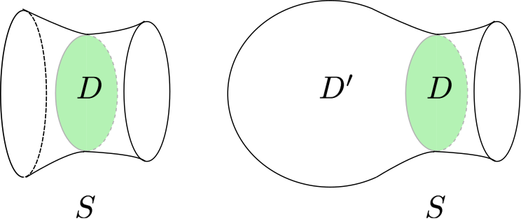
Before stating the main results about this decomposition, we introduce some notation; for full details, we refer the reader to [Mar16]. Let $M$ be a compact, orientable $3$-manifold, and $S\subset M$ a properly embedded orientable surface, i.e. an orientable, embedded surface such that $\partial S\subset\partial M$. A disk $D\subset M$ is called a compressing disc for $S$ if $\partial D=D\cap S$ and $\partial D$ does not bound a disc in $S$. A properly embedded, connected, orientable surface $S\subset M$ with $\chi(S)\leq 0$ is compressible if it has a compressing disc, incompressible otherwise, see Figure 2.2.

Figure 2.2: If the surface $S\subset M$ is incompressible, then for every disc $D\subset M$ such that $\partial D\subset S$ (on the left), there exists a disc $D^{\prime}\subset S$ such that $\partial D^{\prime}=\partial D$ (on the right).

A properly embedded surface $S\subset M$ is $\partial$-parallel if the inclusion $i:S\hookrightarrow M$ is isotopic to a map into the boundary $i_{0}:S^{\prime}\hookrightarrow\partial M$. A surface is essential if it is incompressible and not $\partial$-parallel.

In [Thu82] Thurston introduced the following definition.

Definition 2.5.

An irreducible $3$-manifold is homotopically atoroidal if every $\pi_{1}$-injective map from the torus to the irreducible manifold $X$ is homotopic to a map into the boundary.

It turns out that homotopically atoroidal manifolds are, together with Seifert manifolds, the “building blocks” of the closed, orientable, irreducible $3$-manifolds. This is made precise in the following statement.

JSJ Decomposition Theorem.

Let $Y$ be a closed, orientable, irreducible $3$-manifold. There exist a collection $\mathcal{C}=\{T_{1},\dots,T_{r}\}$ of disjoint, essential tori in the interior of $Y$ enjoing the following properties:

1. every connected component of $Y\setminus\mathcal{C}$ is either a Seifert manifold, or homotopically atoroidal;

2. the collection $\mathcal{C}$ is minimal.

Furthermore, the collection $\mathcal{C}$ is unique up to isotopy.

Notice that statement i. does not provide a dichotomy between Seifert and homotopically atoroidal components of the decomposition. However, if we focus on orientable Seifert fibred manifolds with boundary there are only three manifolds which are both homotopically atoroidal and Seifert: $K\widetilde{\times}I,T^{2}\times I,D^{2}\times S^{1}$. Moreover, the only one that can possibly appear as a $JSJ$ component of a closed, orientable, irreducible $3$-manifolds is $K\widetilde{\times}I$.

In [Thu82], Thurston stated his celebrated Geometrization Conjecture and announced some papers (see [Thu86], [Thu98a], [Thu98b]) proving his conjecture in restriction to Haken manifolds. One of the major steps in the proof is the so called Hyperbolization Theorem, which claims the existence of a complete Riemannian metric, locally isometric to $\mathbb{H}^{3}$ in the interior of non-Seifert fibered irreducible $3$-manifolds. We refer to [Ota96] and [Ota98] for a complete proof of this theorem. Later on, thanks to the work of Perelman (see [Per02], [Per03a] and [Per03b]), it was possible to replace the hypothesis “Haken manifold” with “with infinite fundamental group” in the statement of the Hyperbolization Theorem. We state here the more recent version of the Thoerem:

Hyperbolization Theorem.

The interior of a compact, orientable, irreducible, $3$-manifold $X$ with infinite fundamental group admits a complete, hyperbolic metric if and only if the manifold is homotopically atoroidal and not homeomorphic to $K\widetilde{\times}I$. Moreover, the hyperbolic metric has finite volume if and only if $\partial X$ is a union of tori and $X\not\simeq T^{2}\times I,D^{2}\times S^{1}$.

2.3 Non-positively curved $C^{2}$ metrics on Seifert manifolds

We observed in Chapter 2 that Seifert components of irreducible, orientable, closed $3$-manifolds having at leat a hyperbolic piece in their $JSJ$ decomposition are either of hyperbolic type or homeomorphic to $K\tilde{\times}I$, as $D^{2}\times S^{1}$ and $T^{2}\times I$ cannot appear as $JSJ$ components of closed, irreducible $3$-manifolds. In §LABEL:section_Eberlein we explained how a non-positively curved metric with totally geodesic boundary $g_{0}$ on a Seifert fibred manifold $S$ with base orbifold $\mathcal{O}_{S}$ provides us with a non-positively curved metric with totally geodesic boundary $\bar{g}_{0}$ on the base orbifold. Moreover, the quotient map collapsing the fibres to points is a Riemannian orbifold submersion $p:(S,g_{0})\rightarrow(\mathcal{O}_{S},\bar{g_{0}})$. This section is devoted to the proof of the following proposition:

Proposition 2.6.

For every orientable Seifert manifold with boundary and hyperbolic base orbifold $S=S(g,l;(p_{1},q_{1}),\dots,(p_{k},q_{k}))$, given any compatible collection of metrics $h_{1},\dots,h_{l}$ on the boundary tori $T_{1},\dots,T_{l}$ of $S$, there exist $\bar{\delta}_{S},\bar{\zeta}_{S}(\delta)>0$ with $\bar{\zeta}_{S}(\delta)\rightarrow 0$ as $\delta\rightarrow 0$ and a $2$-parameter family of $C^{2}$ Riemannian metrics $\left\{k_{\delta,\zeta}\right\}_{\delta\in(0,\bar{\delta}_{S}],\zeta\in(0,\bar{\zeta}_{S}(\delta)]}$, such that:

• $-1-\delta\leq\sigma_{\delta,\zeta}\leq 0$, where $\sigma_{\delta,\zeta}$ is the sectional curvature of the metric $k_{\delta,\zeta}$;

• $k_{\delta,\zeta}|_{T_{i}}=\zeta^{2}h_{i}$;

• the metrics are flat in a collar of the boundary;

• $\operatorname{Vol}\left(S,k_{\delta,\zeta}\right)\overset{\delta\rightarrow 0}{\longrightarrow}0$.

Any compatible metric $h_{1}$ on $\partial(K\widetilde{\times}I)$ is the restriction to the boundary of a flat metric $g$. Then the collection $\zeta^{2}g$ for $\zeta\in(0,1]$ is a continuous family of homothetic flat metrics verifying in particular $(i)$—$(iv)$.

Remark 2.7.

Few words about this result:

• with these requirements we are not able to extend any compatible collection of flat metrics on $\partial S$, but any compatible collection has a rescaling which can be extended to a $C^{2}$ Riemannian metric as above;

• in the case where $S$ is a Seifert fibred manifold with hyperbolic base orbifold the bounds on $\sigma_{\delta,\zeta}$ are “$\delta$-almost optimal" in the sense that the upper bound coincides with the upper bound of a geometric metric of finite volume on $int(S)$ and the lower bound is smaller than the lower bound of such a metric by an amount of $\delta$;

• the almost optimal lower bound on the sectional curvature, turns out to be a strong constraint: indeed, it is possible to put smooth, non-positively curved Riemannian metric satisfying conditions $(ii)$—$(iv)$ up to relaxing the condition $(i)$ to $\sigma_{\delta,\zeta}\geq-K^{2}$ for a suitable $K$, but we are not able to find a smooth family of metrics satisfying the bounds in $(i)$;

• if we ask a $\delta$-almost optimal upper bound on the sectional curvature, instead of non-positivity, that is $-1-\delta\leq\sigma_{\delta,\zeta}\leq\delta$, we can improve $C^{2}$ to $C^{\infty}$, using a density argument.

Proof.

First of all, we shall treat separately the case where $\mathcal{O}_{S}$ is a hyperbolic orbifold and the case of $K\widetilde{\times}I$.

Case $\chi_{orb}(\mathcal{O}_{S})<0$. Let $\{h_{1},...,h_{l}\}$ be a collection of compatible metrics on $S$. By definition, there exists on $S$ a metric $g_{0}$ of non-positive curvature such that $(T_{i},g_{0}|_{T_{i}})$ is isometric to $(T_{i},h_{i})$. As we have seen in Section §LABEL:section_Eberlein this gives us a non-positively curved metric $\bar{g}_{0}$ on the base orbifold $\mathcal{O}_{S}$ and a Riemannian orbifold submersion $p:(S,g_{0})\rightarrow(\mathcal{O}_{S},\bar{g}_{0})$. Equivalently, we have a pair of morphisms $\rho_{h}:\pi_{1}(S)\rightarrow\mathrm{Isom}(\widetilde{\mathcal{O}}_{S},\tilde{\bar{g}}_{0})$ and $\rho_{v}:\pi_{1}(S)\rightarrow\mathrm{Isom}(\mathbb{E}^{1})$ such that the pair $(\rho_{h},\rho_{v})$ is an injective morphism of $\pi_{1}(S)$ into $\mathrm{Isom}^{+}((\widetilde{\mathcal{O}}_{S},\tilde{\bar{g}}_{0})\times\mathbb{E}^{1})$, whose action on $(\widetilde{\mathcal{O}}_{S},\tilde{\bar{g}}_{0})\times\mathbb{E}^{1}$ is free and discrete. We recall that, by construction, we have :

— if $g\geq 0$, then $\rho_{v}(a_{i})$, $\rho_{v}(b_{i})$, $\rho_{v}(c_{j})$, $\rho_{v}(d_{r})$ are orientation preserving isometries of $\mathbb{E}^{1}$ —thus translations of $\mathbb{E}^{1}$—, then Leeb’s compatibility condition can be expressed in additive notation (with a slight abuse of notation, since we are identifying the translation thought as an isometry with the amount of the translation itself):

$$\sum_{r=1}^{l}\rho_{v}(d_{r})+\sum_{j=1}^{k}\rho_{v}(c_{j})=0,$$

$$\frac{p_{j}}{q_{j}}\rho_{v}(c_{j})=\rho_{v}(f)\mbox{ for }j=1,...,k;$$

— if $g<0$ we know that the generators $a_{1},...,a_{|g|}$ of $\pi_{1}(S)$ act on each of the two factors of the Riemannian product $(\widetilde{\mathcal{O}}_{S},\tilde{\bar{g}}_{0})\times\mathbb{E}^{1}$ as orientation reversing isometries, this means that $\rho_{v}(a_{i})$, $i=1,..,|g|$ are inversions of $\mathbb{E}^{1}$. Consequently $\rho_{v}(a_{i}^{2})=\rho_{v}(a_{i})^{2}=\operatorname{id}_{\mathbb{E}^{1}}$ for any $i=1,...,|g|$. As the $d_{r}$’s and the $c_{j}$’s act as orientation preserving isometries on both factors we conclude that, also in this case, we can use the additive notation to express the compatibility conditions:

$$\sum_{r=1}^{l}\rho_{v}(d_{r})+\sum_{j=1}^{k}\rho_{v}(c_{j})=0,$$

$$\frac{p_{j}}{q_{j}}\rho_{v}(c_{j})=\rho_{v}(f)\mbox{ for }j=1,...,k;$$

Observe that, if $(\rho_{h},\rho_{v}):\pi_{1}(S)\rightarrow\mathrm{Isom}^{+}((\widetilde{\mathcal{O}}_{S},\tilde{\bar{g}}_{0})\times\mathbb{E}^{1})$ is an injective morphism whose image acts freely and discretely on $(\widetilde{\mathcal{O}}_{S},\tilde{\bar{g}}_{0})\times\mathbb{E}^{1}$, the same holds for $(\rho_{h},\rho_{v}^{\varepsilon}):\pi_{1}(S)\rightarrow\mathrm{Isom}^{+}((\widetilde{\mathcal{O}}_{S},\tilde{\bar{g}}_{0})\times\mathbb{E}^{1})$, where we denoted $\rho_{v}^{\varepsilon}$ the morphism which coincides with $\rho_{v}$ on the generators $a_{i}$’s, $b_{i}$’s if $g\geq 0$ and $a_{i}$’s if $g<0$ and which is a rescaling by a factor $\varepsilon$ of the translations $\rho_{v}(d_{r})$’s, $\rho_{v}(c_{j})$’s and $\rho_{v}(f)$.
For any $r=1,...,l$ we shall denote by $\ell_{r}$ the translation length of $\rho_{h}(d_{r})$, that is, the length of the corresponding boundary component of $(\mathcal{O}_{S},\bar{g}_{0})$. Notice that the translation length of $(\rho_{h}(d_{r}),\rho_{v}(d_{r}))$ is equal to $\sqrt{\ell_{r}^{2}+(\rho_{v}(d_{r}))^{2}}$ and it is attained for all the points of one boundary component of $(\widetilde{S},\tilde{g}_{0})$ which is one of the lifts of the boundary torus $T_{r}$.

Now we shall modify a geometric metric $g$ on $int(S)$ locally isometric to $\mathbb{H}^{2}\times\mathbb{E}^{1}$ in order to obtain the desired collection of $\mathcal{C}^{2}$ metrics $\{k_{\delta,\zeta}\}$ whose curvatures are bounded by $-1-\delta\leq\sigma\leq 0$, with $\delta\longrightarrow 0$, flat near the boundary, such that the restriction $k_{\delta,\zeta}|_{T_{i}}=\zeta^{2}h_{i}$, where $\zeta<\bar{\zeta}_{S}(\delta)$ with $\bar{\zeta}_{S}(\delta)\rightarrow 0$ for $\delta\rightarrow 0$, and whose volumes collapse as $\delta\rightarrow 0$. Once chosen $g$ a complete geometric metric of finite volume on $int(S)$, locally isometric to $\mathbb{H}^{2}\times\mathbb{E}^{1}$, call $\bar{g}$ the corresponding complete hyperbolic metric on $int(\mathcal{O}_{S})$, and $\rho_{g}:\pi_{1}(S)\rightarrow\mathrm{Isom}^{+}(\mathbb{H}^{2}\times\mathbb{E}^{1})$ the injective morphism such that $\mathbb{H}^{2}\times\mathbb{E}^{1}/\rho_{g}(\pi_{1}(S))$ is isometric to $(int(S),g)$.
Let us denote by $\mathcal{C}_{1},\dots,\mathcal{C}_{l}$ the connected components of a horoball neighbourhood of the cusps in $\mathcal{O}_{S}$; observe that by definition it does not contain any conical point (see Appendix A). Fix the parametrization in horospherical coordinates; then $\mathcal{C}_{r}\simeq S^{1}\times[0,+\infty)$. Let $m_{r}$ be the length of the section $\{0\}\times S^{1}$ with respect to the hyperbolic metric. Then the hyperbolic metric on each cusp $\mathcal{C}_{r}$ can be locally written as a warped product:

$$\bar{g}=e^{-2t}m_{r}^{2}\,dx^{2}\oplus dt^{2},$$

where $dx^{2}$ is an Euclidean metric on the horosphere.

Now, let $T_{\delta}=\frac{1}{\delta}$. We shall modify the hyperbolic metric on the cusps starting from time $T_{\delta}$, thus producing the required sequence. Before that, let us state the following proposition whose proof is given in Appendix B.

Proposition 2.8.

For every fixed $\ell,\delta>0$ there exist $\varepsilon,\varepsilon^{\prime}>0$ arbitrarily small and $\varphi_{\varepsilon,\varepsilon^{\prime}}\in C^{2}(\mathbb{R})$ such that:

1. $\varphi_{\varepsilon,\varepsilon^{\prime}}$ is not increasing and convex, such that

   $$\left\{\begin{array}[]{l}\varphi_{\varepsilon,\varepsilon^{\prime}}(t)=\varphi_{0}(t)=\ell e^{-t}\mbox{ for }t\leq-\varepsilon,\\ \varphi_{\varepsilon,\varepsilon^{\prime}}(t)=\ell^{\prime}\mbox{ for }t\geq t_{\delta}+\varepsilon^{\prime},\end{array}\right.$$

   where

   $$\ell\frac{\sqrt{\delta(1+\delta)}}{1+2\delta}\leq\ell^{\prime}(\delta,\varepsilon,\varepsilon^{\prime})\leq 4\ell\frac{\sqrt{\delta(1+\delta)}}{1+2\delta}$$

2. $\left(\dfrac{\varphi_{\varepsilon,\varepsilon^{\prime}}^{\prime}}{\varphi_{\varepsilon,\varepsilon^{\prime}}}\right)^{2}<(1+2\delta)^{2}\left(\dfrac{\varphi_{0\phantom{,^{\prime}}}^{\prime}}{\varphi_{0\phantom{,^{\prime}}}}\right)^{2}$ for every $t\in\mathbb{R}$;

3. $\dfrac{\varphi_{\varepsilon,\varepsilon^{\prime}}^{\prime\prime}}{\varphi_{\varepsilon,\varepsilon^{\prime}}}\leq(1+2\delta)^{2}$ for every $t\in(-\varepsilon,t_{\delta}+\varepsilon^{\prime})$.

where $t_{\delta}=\frac{1}{2(1+2\delta)}\ln\left(1+\frac{1}{\delta}\right)$.

Now, let $\varphi_{\delta,r}$ be the $C^{2}$ function on $[0,T_{\delta}+t_{\delta}+2\varepsilon^{\prime}]$ which coincides with $e^{-t}m_{r}$ for $t\in[0,T_{\delta}-\varepsilon]$ and with $\varphi_{\varepsilon,\varepsilon^{\prime}}$ given by Proposition 2.8 for $\ell=e^{-T_{\delta}}m_{r}$ for $t\in[T_{\delta}-\varepsilon,T_{\delta}+t_{\delta}+2\varepsilon^{\prime}]$. Then, substitute the warping function $m_{r}e^{-t}$ on $S^{1}\times[0,T_{\delta}+t_{\delta}+2\varepsilon^{\prime}]$ with the new function $\varphi_{\delta,r}$, thus obtaining the metric

$$\bar{g}_{\delta}=\varphi_{\delta,r}^{2}dx^{2}\oplus dt^{2}.$$

For any fixed $\delta$ this gives us a $C^{2}$ Riemannian metric $\bar{g}_{\delta}$ satisfying the required bounds on the sectional curvature, which is hyperbolic on the complement of the horoball neighbourhoods $\mathcal{C}_{r}(T_{\delta})\simeq S^{1}\times[T_{\delta},+\infty)$ and flat near the boundary. Nevertheless, condition $ii$ is not verified, hence, we shall adjust the metric $g_{\delta}$ along the cusps, and we shall give an explicit value of $\varepsilon(\delta)$ of point $ii$. Let us remark that $\ell^{\prime}$ of Proposition 2.8 continuously depends on $(\delta,\varepsilon,\varepsilon^{\prime})$, and goes to $0$ as $(\delta,\varepsilon,\varepsilon^{\prime})\rightarrow(0,0,0)$. In particular, for every

$$\zeta\leq\bar{\zeta}(\delta,S,\{h_{i}\})=\frac{1}{2}\cdot\min_{i=1,..,l}\left\{\frac{\ell_{r}^{\prime}(\delta,\varepsilon,\varepsilon^{\prime})}{\ell_{r}}\right\}$$

we can find a suitable $3$-tuple $(\delta_{r}(\zeta),\varepsilon_{r}(\zeta),\varepsilon_{r}^{\prime}(\zeta))$ so that for every cusp we have $\ell_{r}^{\prime}=\zeta\cdot\ell_{r}$. Let us call $\bar{k}_{\delta,\zeta}$ the previous metric and let us denote by $\bar{\rho}_{\delta,\zeta}:\pi_{1}(\mathcal{O}_{S})\rightarrow\mathrm{Isom}(\widetilde{O}_{S},\tilde{\bar{k}}_{\delta,\zeta})$ the corresponding injective homomorphism. It is worth to notice that, integrating along the cusps, we get

$$\operatorname{Vol}(\mathcal{O}_{S},\bar{k}_{\delta,\zeta})\leq\operatorname{Vol}(int(\mathcal{O}_{S}),\bar{g})+\sum_{r=1}^{l}\int_{T_{\delta_{r}}-\varepsilon_{r}}^{T_{\delta_{r}}+t_{\delta_{r}}+2\varepsilon_{r}^{\prime}}\varphi_{\delta_{r},r}dt\leq$$

$$\leq\operatorname{Vol}(int(\mathcal{O}_{S}),\bar{g})+\sum_{r=1}^{l}e^{-(\frac{1}{\delta_{r}}-1)}\left(\frac{\ln(1+\frac{1}{\delta_{r}})}{2(1+2\delta_{r})}+1\right)\longrightarrow\operatorname{Vol}(int(\mathcal{O}_{S}),\bar{g})$$

when $\delta_{1},\dots,\delta_{l}\rightarrow 0$.
To conclude, consider $(\bar{\rho}_{\delta,\zeta}\circ p_{*},\rho_{v}^{\zeta}):\pi_{1}(S)\rightarrow\mathrm{Isom}^{+}((\widetilde{O}_{S},\tilde{\bar{k}}_{\delta,\zeta})\times\mathbb{E}^{1})$ and observe that the induced Riemannian metric $k_{\delta,\zeta}$ clearly verifies conditions $i$—$iii$, while condition $iv$ follows from:

$$\operatorname{Vol}(S,k_{\delta,\zeta})=\operatorname{Vol}(\mathcal{O}_{S},\bar{k}_{\delta,\zeta})\cdot\zeta\cdot|\rho_{v}(f)|\overset{\delta\rightarrow 0}{\longrightarrow}0$$

Case $S=K\widetilde{\times}I$. Now suppose that $\chi_{orb}(\mathcal{O}_{S})=0$. Then the Seifert manifold $S$ is $K\widetilde{\times}I$, and can be viewed as $Mb\widetilde{\times}S^{1}$, having the Möbius band as base orbifold (surface) and no singular points. We write down presentations for the (orbifold) fundamental groups:

$$\pi_{1}^{orb}(\mathcal{O}_{S})=\pi_{1}(Mb)=\left\langle\bar{a},\bar{d}\left\lvert\right.\bar{a}^{2}=\bar{d}\right\rangle\simeq\mathbb{Z}$$

$$\pi_{1}(K\widetilde{\times}I)=\left\langle a,d,f\left\lvert\begin{array}[]{l}{a}^{2}={d}\\ {a}f{a}^{-1}=f^{-1}\end{array}\right.\right\rangle$$

Observe that a flat metric on the boundary torus of $K\widetilde{\times}I$ is compatible if and only if is the restriction to the boundary of a flat metric $g$ on $K\widetilde{\times}I$. Indeed, a non-flat, non positively curved metric $g$ on $K\widetilde{\times}I$ flat on a collar of the boundary would give a non-positively curved metric on $(D(K\widetilde{\times}I),g^{\prime})$, the Riemannian manifold obtained by doubling $(K\widetilde{\times}I,g)$ along the boundary torus. But $D(K\widetilde{\times}I)$ is finitely covered by a $3$-dimensional torus $T^{3}$, and this would give a contradiction since $\hat{g}^{\prime}$, the lift of the metric $g^{\prime}$ would be a non-positively curved, non-flat metric on $T^{3}$. The flat metric $g$ on $K\widetilde{\times}I$ is obtained as the quotient of $([-a,a]\times\mathbb{E}^{1})\times\mathbb{E}^{1}$ (for a suitable choice of $a$) by the isometry subgroup given by the image of the following injective homomorphism:

$$\begin{array}[]{cccc}\rho=(\rho_{h},\rho_{v}):&\pi_{1}(Mb\times S^{1})&\longrightarrow&\operatorname{Isom}^{+}(([-a,a]\times\mathbb{E}^{1})\times\mathbb{E}^{1})\\ &{a}&\longmapsto&(\rho_{h}(a),\rho_{v}({a}))\\ &f&\longmapsto&(\mbox{ Id }\;,\rho_{v}(f))\end{array}$$

where $\rho_{h}(a)$ is the glide-reflection $(x,y)\mapsto(-x,ky)$, for $k\in\mathbb{R}$ and $\rho_{v}(a)$ is a the symmetry with respect to a point in $\mathbb{E}^{1}$. As usual $\rho(f)$ acts as the identity on the first component $([-a,a]\times\mathbb{E}^{1})$ and as a translation $\rho_{v}(f)$ on $\mathbb{E}^{1}$. Observe that the isometries $\rho(a^{2})$ and $\rho(f)$ act fixing both boundary components of $([-a,a]\times\mathbb{E}^{1})\times\mathbb{E}^{1}$ and that $\rho(a^{2})=(\rho_{h}(a^{2}),\operatorname{Id}_{\mathbb{E}^{1}})$ with $\rho_{h}(a^{2})(x,y)=(x,2k\,y)$. In other words, given the previous presentation of $\pi_{1}(K\widetilde{\times}I)$ the elements $a^{2}$ and $f$ act as translations along orthogonal directions on the universal covering: hence a compatible metric $h_{1}$ on $\partial(K\widetilde{\times}I)$ is necessarily a flat metric generated by an orthogonal lattice (given by restricting $\langle\rho(a^{2}),\rho(f)\rangle$ to an isometry of $\mathbb{E}^{1}\times\mathbb{E}^{1}$). Rescalings of $g$ provides $K\widetilde{\times}I$ with the required family of Riemannian metrics. ∎

2.4 Metrics of non-positive curvature
on atoroidal $3$-manifolds

The main result of this section is the following:

Theorem 2.9.

Let $X$ be a hyperbolic component and let $\{h_{r}\}_{r=1}^{l}$ be a flat metric on the boundary of $X$. There exists a sequence of metrics $hyp_{\delta}^{0}$ on $X$ such that:

1. For every $\delta$ the sectional curvature $\sigma_{\delta}^{0}$ is pinched:

   $$-(1+2\delta)^{2}\leq\sigma_{\delta}^{0}\leq 0$$

2. $\operatorname{Vol}(X,hyp_{\delta}^{0})\overset{\delta\rightarrow 0}{\longrightarrow}\operatorname{Vol}(int(X),hyp)$, where $hyp$ it the unique —up to isometry— complete, finite volume hyperbolic metric on $int(X)$.

3. There exists a family $\{\mathcal{U}_{\delta}\}_{\delta\in(0,1]}$ of nested horoball neighbourhoods of the cusps of $(int(X),hyp)$, whose complements for $\delta\rightarrow 0$ progressively exhaust $(int(X),hyp)$, such that $(int(X)\smallsetminus\mathcal{U}_{\delta},hyp)$ is isometric to an open set $V_{\delta}$ in $(X,hyp_{\delta}^{0})$ and such that $\frac{\operatorname{Vol}(X,hyp_{\delta}^{0})}{\operatorname{Vol}(V_{\delta},hyp_{\delta}^{0})}\rightarrow 1$.

4. The metric $hyp_{\delta}^{0}$ is flat in a collar of the boundary and there exists $\ell^{\prime}=\ell^{\prime}(X,\delta,\{h_{i}\})$ such that $(T_{i},hyp_{\delta}^{0}|_{T_{i}})$ is isometric to $(T_{i},(\ell^{\prime})^{2}h_{i})$.

In order to achieve this result we will prove a the following lemma, which is a refinement of part of the argument given by Leeb to prove [Lee95], Proposition 2.3.

Lemma 2.10.

Let $(X^{\prime},hyp)$ be an open $3$-manifold endowed with a complete Riemannian metric of finite volume, locally isometric to $\mathbb{H}^{3}$. Let

$$\mathcal{U}=\bigcup_{i=1}^{r}\mathcal{C}_{i}=\bigcup_{i=1}^{r}T_{i}\times[0,\infty)$$

be a horoball neighbourhood of the cusps of $(X^{\prime},hyp)$. Let $h_{1},\dots,h_{r}$ be a collection of flat metrics on $T_{1},\dots,T_{r}$. There exists a $1$-parameter family of complete Riemannian metrics $\{hyp_{\delta}\}_{\delta\in(0,1]}$ with the following properties:

1. $-1-\delta\leq\sigma_{\delta}\leq-1$;

2. $hyp_{\delta}=hyp$ on $X^{\prime}\smallsetminus\mathcal{U}_{\delta}$, where $\mathcal{U}_{\delta}=\bigcup_{i=1}^{r}T_{i}\times{[T_{\delta},+\infty)}\subset\mathcal{U}$, for $T_{\delta}=\frac{C}{\delta}$ and where the constant $C$ is determined by $(X^{\prime},hyp)$, $\{h_{i}\}$ and $\mathcal{U}$;

3. $\sigma_{\delta}=-1$ in $(\mathcal{U}_{\delta}^{\prime},hyp_{\delta})$ where $\mathcal{U}_{\delta}^{\prime}=\bigcup_{i=1}^{r}T_{i}\times{[2T_{\delta},+\infty)}$;

4. for $t\geq 2T_{\delta}$ the Riemannian manifold $(T_{i}\times\{t\},hyp_{\delta}|_{T_{i}\times\{t\}})$ is isometric to $(T_{i},\zeta^{2}e^{-2t}h_{i})$ where $\zeta$ is determined by $(X^{\prime},hyp)$, by the collection $\{h_{i}\}$ and the choice of $\mathcal{U}$;

5. $\operatorname{Vol}(X^{\prime},hyp_{\delta})\overset{\delta\rightarrow 0}{\longrightarrow}\operatorname{Vol}(X^{\prime},hyp)$.

Proof.

Let us start with a complete hyperbolic metric of finite volume $hyp$ on $X^{\prime}$. Let $\mathcal{U}$ be the horoball neighbourhood of the cusps of $(X^{\prime},hyp)$ defined in the statement. We know that $hyp$ is given in horospherical coordinates on $\mathcal{C}_{i}$ by:

$$\mathcal{C}_{i}=T_{i}\times[0,+\infty),\quad hyp_{(x,t)}=e^{-2t}(k_{i})_{x}\oplus dt^{2}$$

where $k_{i}$ is determined up to rescaling solely by the metric $hyp$ on $X^{\prime}$, which by Mostow’s rigidity theorem is unique, and is thus independent of the choice of the horoball neighbourhood of the cusps $\mathcal{U}$.
Now we shall change the warping function describing the hyperbolic metric on $\mathcal{U}$ following Leeb’s argument. Let us consider the flat metrics $k_{i}$, $h_{i}$ on $T_{i}$; by the Spectral Theorem it is possible to find a coordinate system $(x_{i},y_{i})$ for $T_{i}$ such that $k_{i}=dx_{i}^{2}\oplus dy_{i}^{2}$ and $h_{i}=a_{i}\,dx_{i}^{2}+b_{i}\,dy_{i}^{2}$ where $a_{i},b_{i}>0$ are two positive real constants. Up to rescaling the metrics $h_{i}$ by the constant $\zeta^{2}=\frac{1}{2}\max_{i=1,..,r}\{\frac{1}{a_{i}},\frac{1}{b_{i}}\}$ we have $0<\zeta^{2}a_{i},\,\zeta^{2}b_{i}<1$ for every $i=1,...,r$.

Let $\phi:\mathbb{R}\rightarrow\left[0,\infty\right]$ be the following function

$$\phi(t)=\left\{\begin{array}[]{cl}1&\mbox{ for }t\leq 0\\ \dfrac{e^{-\frac{1}{1-t}}}{e^{-\frac{1}{1-t}}+e^{-\frac{1}{t}}}&\mbox{ for }t\in(0,1)\\ 0&\mbox{ for }t\geq 1\end{array}\right.$$

Now we define the following functions, which will be the new warping functions for the metric along the cusps:

$$\eta_{a_{i}}^{\delta}(t)=e^{-t}\left(\phi\left(\dfrac{t-T_{\delta}}{T_{\delta}}\right)+\left(1-\phi\left(\dfrac{t-T_{\delta}}{T_{\delta}}\right)\right)\zeta^{2}a_{i}\right),$$

$$\eta_{b_{i}}^{\delta}(t)=e^{-t}\left(\phi\left(\dfrac{t-T_{\delta}}{T_{\delta}}\right)+\left(1-\phi\left(\dfrac{t-T_{\delta}}{T_{\delta}}\right)\right)\zeta^{2}b_{i}\right)$$

where $T_{\delta}$ will be suitably chosen later on. Then consider the following metrics on the $\mathcal{C}_{i}$’s:

$$g_{i}^{\delta}(x_{i},y_{i},t)=(\eta_{a_{i}}^{\delta}(t))^{2}dx_{i}^{2}\oplus(\eta_{b_{i}}^{\delta}(t))^{2}dy_{i}^{2}\oplus dt^{2}$$

Notice that the metrics $g_{i}^{\delta}$ coincide with $hyp$ on $T_{i}\times[0,T_{\delta}]$ and are equal to $e^{-2t}\zeta^{2}h_{i}\oplus dt^{2}$ on $T_{i}\times[2T_{\delta},+\infty)$. Now we shall compute the sectional curvature of the metric $hyp_{\delta}$ obtained by gluing in the obvious way the metrics $g_{i}^{\delta}$ along the cusps. By construction the sectional curvature is constantly equal to $-1$ except on the portions $T_{i}\times[T_{\delta},2T_{\delta}]$ of the cusps. Hence we will need to compute the sectional curvature of the metrics $g_{i}^{\delta}$ only in restriction to $T_{i}\times[T_{\delta},2T_{\delta}]$. An explicit computation of the Christoffel’s symbols for $g_{i}^{\delta}$ gives:

$$\Gamma^{t}_{x_{i}x_{i}} = \frac{1}{2}\left(-\frac{\partial}{\partial t}(\eta_{a_{i}}^{\delta})^{2}\right)$$

$$\Gamma^{t}_{y_{i}y_{i}} = \frac{1}{2}\left(-\frac{\partial}{\partial t}(\eta_{b_{i}}^{\delta})^{2}\right)$$

$$\Gamma^{x_{i}}_{tx_{i}}=\Gamma^{x_{i}}_{x_{i}t} = \frac{1}{2}\frac{1}{(\eta_{a_{i}}^{\delta})^{2}}\left(\frac{\partial}{\partial t}(\eta_{a_{i}}^{\delta})^{2}\right)$$

$$\Gamma^{y_{i}}_{ty_{i}}=\Gamma^{y_{i}}_{y_{i}t} = \frac{1}{2}\frac{1}{(\eta_{b_{i}}^{\delta})^{2}}\left(\frac{\partial}{\partial t}(\eta_{b_{i}}^{\delta})^{2}\right)$$

and zero for all the remaining Christoffel symbols. Thus the sectional curvatures of $g_{i}^{\delta}$ are given by the following formulas:

$$\sigma_{x_{i}y_{i}}^{\delta}=-\frac{({\eta^{\delta}_{a_{i}})}^{\prime}\cdot{(\eta_{b_{i}}^{\delta})}^{\prime}}{{(\eta_{a_{i}}^{\delta})}\cdot{(\eta_{b_{i}}^{\delta})}},\quad\sigma_{x_{i}t}^{\delta}=-\frac{({\eta_{a_{i}}^{\delta}})^{\prime\prime}}{({\eta_{a_{i}}^{\delta}})},\quad\sigma_{y_{i}t}^{\delta}=-\frac{({\eta_{b_{i}}^{\delta}})^{\prime\prime}}{{(\eta_{b_{i}}^{\delta})}}$$

Let us compute the derivatives of $\eta_{a_{i}}^{\delta}$ up to the second order (those of $\eta_{b_{i}}^{\delta}$ are analogous):

$$({\eta_{a_{i}}^{\delta}})^{\prime}(t)=e^{-t}\left(\left(1-\zeta^{2}a_{i}\right)\left(\frac{\phi^{\prime}\left(\frac{t-T_{\delta}}{T_{\delta}}\right)}{T_{\delta}}-\phi\left(\frac{t-T_{\delta}}{T_{\delta}}\right)\right)-\zeta^{2}a_{i}\right)$$

$$({\eta_{a_{i}}^{\delta}})^{\prime\prime}(t)=e^{-t}\left((1-\zeta^{2}a_{i})\left(\frac{\phi^{\prime\prime}\left(\frac{t-T_{\delta}}{T_{\delta}}\right)}{T_{\delta}^{2}}-\frac{2\phi^{\prime}\left(\frac{t-T_{\delta}}{T_{\delta}}\right)}{T_{\delta}}+\phi\left(\frac{t-T_{\delta}}{T_{\delta}}\right)\right)+\zeta^{2}a_{i}\right)$$

Notice that $(\eta_{a_{i}}^{\delta})^{\prime}$, $(\eta_{b_{i}}^{\delta})^{\prime}\leq 0$. We shall now give conditions on $T_{\delta}$ which ensure that $\sigma_{x_{i}t}^{\delta},\sigma_{y_{i}t}^{\delta},\sigma_{x_{i}y_{i}}^{\delta}$ are between $-1-\delta$ and $-1$.

Let us start with the curvature $\sigma_{x_{i}y_{i}}^{\delta}$. We want to give conditions on $T_{\delta}$ so that:

$$-1-\delta\leq\sigma_{x_{i}y_{i}}^{\delta}\leq-1$$

The second inequality is equivalent to:

$$\frac{\left[\left(1-\zeta^{2}a_{i}\right)\left(\phi-\frac{\phi^{\prime}}{T_{\delta}}\right)+\zeta^{2}a_{i}\right]\left[\left(1-\zeta^{2}b_{i}\right)\left(\phi-\frac{\phi^{\prime}}{T_{\delta}}\right)+\zeta^{2}b_{i}\right]}{\left[\left(1-\zeta^{2}a_{i}\right)\phi+\zeta^{2}a_{i}\right]\left[\left(1-\zeta^{2}b_{i}\right)\phi+\zeta^{2}b_{i}\right]}\geq 1$$

where $\phi$, $\phi^{\prime}$ are evaluated at $(t-T_{\delta})/T_{\delta}$. We notice that, since $\phi$ is non-increasing, the previous ratio is always greater then or equal to $1$, independently on the choice of $T_{\delta}$. Thus inequality $\sigma_{x_{i}y_{i}}^{\delta}\leq-1$ actually holds. Now we shall deal with the first inequality $\sigma_{x_{i}y_{i}}^{\delta}\geq-1-\delta$. Remark that:

$$\left(1-\zeta^{2}a_{i}\right)\left(\phi-\frac{\phi^{\prime}}{T_{\delta}}\right)+\zeta^{2}a_{i}\overset{T_{\delta}\rightarrow+\infty}{\longrightarrow}\left(1-\zeta^{2}a_{i}\right)\phi+\zeta^{2}a_{i}$$

$$\left(1-\zeta^{2}b_{i}\right)\left(\phi-\frac{\phi^{\prime}}{T_{\delta}}\right)+\zeta^{2}b_{i}\overset{T_{\delta}\rightarrow+\infty}{\longrightarrow}\left(1-\zeta^{2}b_{i}\right)\phi+\zeta^{2}b_{i}$$

Moreover, an easy calculation shows that condition

$$T_{\delta}\geq\frac{4}{\delta}\cdot\max_{i=1,..,r}\left\{\frac{(1-\zeta^{2}a_{i})}{\zeta^{2}a_{i}},\frac{(1-\zeta^{2}b_{i})}{\zeta^{2}b_{i}}\right\}$$

ensures that $\sigma_{x_{i}y_{i}}^{\delta}\geq-1-\delta$ for every $i=1,...,r$.

Now we shall prescribe the bounds on $\sigma_{x_{i}t}^{\delta}$, to derive the conditions on $T_{\delta}$. We ask:

$$-1-\delta\leq\sigma_{x_{i}t}^{\delta}\leq-1$$

The first inequality is equivalent to:

$$\frac{\left(1-\zeta^{2}a_{i}\right)\left[\frac{1}{T_{\delta}^{2}}\phi^{\prime\prime}-\frac{2}{T_{\delta}}\phi^{\prime}+\phi\right]+\zeta^{2}a_{i}}{\left(1-\zeta^{2}a_{i}\right)\phi+\zeta^{2}a_{i}}\leq 1+\delta$$

where $\phi,\phi^{\prime},\phi^{\prime\prime}$ are computed in $(t-T_{\delta})/T_{\delta}$. Denote by $M^{\prime\prime}=\max_{t\in\left[0,1\right]}\phi^{\prime\prime}$; then a straightforward computation shows that inequality $-1-\delta\leq\sigma_{x_{i}t}^{\delta}$ holds provided that

$$T_{\delta}\geq\frac{1}{\delta}\left(\frac{M^{\prime\prime}+4}{\zeta^{2}a_{i}}\right)$$

For the second inequality, notice that, since $\phi^{\prime\prime}\geq 0$ on $[\frac{1}{2},+\infty)$ and $\phi^{\prime}\leq 0$ we only need to look at the ratio defining $\sigma_{x_{i}t}^{\delta}$ on $T_{i}\times[T_{\delta},2T_{\delta}]$. Let us denote by $m^{\prime\prime}=\min\phi^{\prime\prime}$ then, it is sufficient to choose $T_{\delta}$ such that:

$$\frac{m^{\prime\prime}}{T_{\delta}^{2}}+\frac{4}{T_{\delta}}\geq 0\iff\frac{4}{T_{\delta}}\geq\frac{-m^{\prime\prime}}{T_{\delta}^{2}}\iff T_{\delta}\geq\sqrt{\frac{-m^{\prime\prime}}{4}}$$

Thus, the sectional curvature $\sigma_{x_{i}t}^{\delta}$ is pinched as required provided that

$$T_{\delta}\geq\max\left\{\frac{1}{\delta}\left(\frac{M^{\prime\prime}+4}{\zeta^{2}a_{i}}\right),\sqrt{\frac{-m^{\prime\prime}}{4}}\right\}$$

Analogously, the condition

$$T_{\delta}\geq\max\left\{\frac{1}{\delta}\left(\frac{M^{\prime\prime}+4}{\zeta^{2}b_{i}}\right),\sqrt{\frac{-m^{\prime\prime}}{4}}\right\}$$

ensures that inequalities $-1-\delta\leq\sigma_{y_{i}t}^{\delta}\leq\delta$ hold.

It follows by the discussion about curvatures that, for $\delta<1$, choosing

$$T_{\delta}\geq\frac{1}{\delta}\cdot\max_{i=1,..,r}\left\{\frac{4(1-\zeta^{2}a_{i})}{\zeta^{2}a_{i}},\frac{4(1-\zeta^{2}b_{i})}{\zeta^{2}b_{i}},\frac{M^{\prime\prime}+4}{\zeta^{2}a_{i}}\frac{M^{\prime\prime}+4}{\zeta^{2}b_{i}},\sqrt{\frac{-m^{\prime\prime}}{4}}\right\}=\frac{C}{\delta}$$

where the constant $C$ only depends on $(X^{\prime},hyp)$, $\{h_{i}\}_{i=1}^{r}$ and on the choice of the original horoball neighbourhood $\mathcal{U}$, the sectional curvatures are pinched as required in the statement. From now on we shall consider $T_{\delta}=\frac{C}{\delta}$. With this proviso, the metric $hyp_{\delta}$ verifies properties $(1)$—$(4)$.

Finally, we have to check Property $(5)$, concerning the convergence of the volumes. Let us denote by $\overline{V}_{T_{\delta}}$ the volume of $(X^{\prime}\smallsetminus\mathcal{U}_{\delta},hyp)$, by $V_{1}(\delta)$ the sum of the volumes respect of the warped toroidal cylinders $(T_{i}\times[T_{\delta},2T_{\delta}],hyp_{\delta})$ and by $V_{2}(\delta)$ the sum of the volumes of $(T_{i}\times[2T_{\delta},+\infty],hyp_{\delta})$. With this notation:

$$\operatorname{Vol}(X^{\prime},hyp_{\delta})=\overline{V}_{g_{0},T_{\delta}}+V_{1}(\delta)+V_{2}(\varepsilon).$$

By construction $\overline{V}_{T_{\delta}}\overset{\delta\rightarrow 0}{\longrightarrow}\operatorname{Vol}(X^{\prime},hyp)$. For any $i=1,\dots,r$ and any $t\geq T_{\delta}$ we denote by $\mathcal{A}_{i}(\delta,t)=\mathcal{A}(T_{i}\times\{t\},hyp_{\delta})$ the area of $T_{i}\times\{t\}$ with respect to the restriction of the metric $hyp_{\delta}$. Then:

$$V_{1}(\delta)=\sum_{i=1}^{r}\int_{T_{\delta}}^{2T_{\delta}}e^{-2t}\cdot\mathcal{A}_{i}(\delta,t)dt.$$

Now observe that for $t\in[T_{\delta},2T_{\delta}]$,

$$\mathcal{A}_{i}(\delta,t)=\mathcal{A}\left(T_{i},\phi\left(\frac{t-T_{\delta}}{T_{\delta}}\right)k_{i}+\left(1-\phi\left(\frac{t-T_{\delta}}{T_{\delta}}\right)\right)\zeta^{2}h_{i}\right).$$

We define:

$$A=\max_{i}\max_{t\in\left[0,1\right]}\mathcal{A}\left(T_{i},\phi(t)k_{i}+(1-\phi(t))\zeta^{2}h_{i}\right).$$

Then:

$$V_{1}(\delta)=\sum_{i=1}^{r}\int_{T_{\delta}}^{2T_{\delta}}e^{-2t}\cdot\mathcal{A}_{i}(\delta,t)dt\leq rA\cdot\int_{T_{\delta}}^{2T_{\delta}}e^{-2t}=rA\huge\left[-\frac{e^{-2t}}{2}\huge\right]_{T_{\delta}}^{2T_{\delta}}=$$

$$=rAe^{-T_{\delta}}\left(\frac{1}{2}-\frac{e^{-T_{\delta}}}{2}\right)\overset{\varepsilon\rightarrow 0}{\longrightarrow}0$$

Finally, we give an estimate for $V_{2}(\delta)$. Let $V_{max}=\max_{i=1,..,r}\mathcal{A}(T_{i},\zeta^{2}h_{i})$, then:

$$V_{2}(\delta)\leq\int_{2T_{\delta}}^{+\infty}e^{-2t}V_{max}dt=V_{max}\cdot\left[-\frac{e^{-2t}}{2}\right]_{2T_{\delta}}^{+\infty}=V_{max}\,\frac{e^{-4T_{\delta}}}{2}\overset{\delta\rightarrow 0}{\longrightarrow}0$$

Since for $\delta\rightarrow 0$ we have $\overline{V}_{T_{\delta}}\rightarrow\operatorname{Vol}(X^{\prime},hyp)$, $V_{1}(\delta)\rightarrow 0$ and $V_{2}(\delta)\rightarrow 0$, we conclude:

$$\operatorname{Vol}(X^{\prime},hyp_{\delta})\overset{\delta\rightarrow 0}{\longrightarrow}\operatorname{Vol}(X^{\prime},hyp)$$

∎

Proof of Theorem 2.9.

Let $X$ be a compact, irreducible, orientable, $3$-manifold with non-empty toroidal boundary $\partial X=T_{1},..,T_{r}$, whose interior $int(X)$ admits a complete hyperbolic metric $hyp$ of finite volume. Fix a horoball neighbourhood $\mathcal{U}$ of the cusps of $(int(X),hyp)$ (as in the statement of Lemma 2.10). Hence, Lemma 2.10 provides us with a continuous $1$-parameter family of complete Riemannian metrics $hyp_{\delta}$, satisfying $(1)$—$(5)$. Let the horoball neighbourhood $\mathcal{U}$ be parametrized as:

$$\mathcal{U}=\bigcup_{i=1}^{r}T_{i}\times[0,+\infty)$$

Then, the metrics $hyp_{\delta}$ in restriction to $T_{i}\times[2T_{\delta},+\infty)$ can be written as $e^{-2t}\zeta^{2}h_{i}\oplus dt^{2}$. We shall now apply Proposition 2.8 for $\ell=\zeta e^{-3T_{\delta}}$ and $\delta$: there exists a $C^{2}$ function $\varphi_{\varepsilon,\varepsilon^{\prime}}$ (where $\varepsilon,\varepsilon^{\prime}$ are sufficiently small positive constants) such that

1. $\varphi_{\varepsilon,\varepsilon^{\prime}}$ is not increasing and convex;

2. $\varphi_{\varepsilon,\varepsilon^{\prime}}$ verifies

   $$\left\{\begin{array}[]{l}\varphi_{\varepsilon,\varepsilon^{\prime}}(t)=\varphi_{0}(t)=\ell e^{-t}\mbox{ for }t\leq-\varepsilon\\ \varphi_{\varepsilon,\varepsilon^{\prime}}(t)=\ell^{\prime}\mbox{ for }t\geq t_{\delta}+\varepsilon^{\prime}\end{array}\right.$$

   where: $\ell\frac{\sqrt{\delta(1+\delta)}}{1+2\delta}\leq\ell^{\prime}=\ell^{\prime}(\delta,\varepsilon,\varepsilon^{\prime})\leq 4\ell\frac{\sqrt{\delta(1+\delta)}}{1+2\delta}$.

3. $\left(\dfrac{\varphi_{\varepsilon,\varepsilon^{\prime}}^{\prime}}{\varphi_{\varepsilon,\varepsilon^{\prime}}}\right)^{2}\leq(1+2\delta)^{2}$ for every $t\in\mathbb{R}$;

4. $\dfrac{\varphi_{\varepsilon,\varepsilon^{\prime}}^{\prime\prime}}{\varphi_{\varepsilon,\varepsilon^{\prime}}}\leq(1+2\delta)^{2}$ for every $t\in(-\varepsilon,t_{\delta}+\varepsilon^{\prime})$.

where $t_{\delta}=\frac{1}{2(1+2\delta)}\ln\left(1+\frac{1}{\delta}\right)$. Now, let $\varphi_{i,\delta}(t)=\zeta e^{-t}$ for $t\in[2T_{\delta},\frac{5T_{\delta}}{2}]$ and $\varphi_{i,\delta}(t)=\varphi_{\varepsilon,\varepsilon^{\prime}}(t)$ for $t\in[\frac{5T_{\delta}}{2},3T_{\delta}+2t_{\delta}]$. Then glue the Riemannian metric $hyp_{\delta}$ in restriction to $T_{i}\times[0,\frac{5T_{\delta}}{2}]$ to the Riemannian $C^{2}$ metric given by $\varphi_{i,\delta}(t)^{2}h_{i}\oplus dt^{2}$ on $[2T_{\delta},3T_{\delta}+2t_{\delta}]$; remark that both metrics on $T_{i}\times[T_{\delta},2T_{\delta}]$ have the form $e^{-2t}\zeta^{2}h_{i}\oplus dt^{2}$ by construction. The result of these gluings for any $i=1,...,r$ produces a $C^{2}$ Riemmanian metric $hyp_{\delta}^{0}$ on $X$ satisfying properties $(1)$—$(4)$. Properties $(1)$, $(3)$, $(4)$ are straightforward from the construction; to check property $(2)$ one needs to adapt the argument for the volume convergence from Proposition 2.6 and use it in combination with Lemma 2.10, $(5)$. ∎

2.5 An upper bound to MinEnt

In this last section of Chapter 3 we shall give a proof of Theorem LABEL:thm_construction_sequence_on_irreducible_Y, thus exhibiting a sequence of $C^{2}$ Riemannian metrics of non-positive sectional curvatures converging to the conjectural value of the Minimal Entropy of $Y$.

Proof of Theorem LABEL:thm_construction_sequence_on_irreducible_Y.

Since $Y$ is a closed irreducible, orientable $3$-manifold, with non-trivial $JSJ$ decomposition and at least one hyperbolic $JSJ$-component, we know that there exists a $JSJ$ compatible collection of flat metrics $\{\{h_{i,j}\}_{j=1,..,l_{i}}\}_{i=1,...,n}$ on the boundary components $\partial X_{i}$’s of the $JSJ$ components of $Y$. By Proposition 2.6 and Theorem 2.9 we know that for any choice of $\delta$ there exists a suitable $\bar{\zeta}(\delta)$ depending on $Y$ and the $JSJ$ compatible collection $\{h_{i,j}\}$ such that:

• on every hyperbolic $JSJ$ component $X_{i}$, $i=1,..,k$ of $Y$ there exists a metric $hyp_{i,\delta}^{0}$ verifying $(1)$–$(3)$ and $(4)$ for the constant $\ell^{\prime}=\bar{\zeta}(\delta)$;

• on every Seifert fibred $JSJ$ component $X_{i}$, $i=k+1,...,n$ of $Y$ there exists a metric $k_{\delta,\bar{\zeta}(\delta)}^{i}$ satisfying properties $(i)$—$(iv)$;

By construction and $JSJ$ compatibility of the $\{h_{i,j}\}$ collection these metrics on the $JSJ$ components fit together to produce a non-positively curved $C^{2}$ Riemannian metric $g_{\delta}$ on $Y$ with the following properties:

1. $-(1+2\delta)^{2}\leq\sigma_{\delta}\leq 0$;

2. $\operatorname{Vol}(Y,g_{\delta})=\sum_{i=1}^{k}\operatorname{Vol}(X_{i},hyp_{i,\delta}^{0})+\sum_{i=k+1}^{n}\operatorname{Vol}(X_{i},k_{\delta,\bar{\zeta}(\delta)}^{i})$ so that, by what has been proved in Proposition 2.6 and Theorem LABEL:thm_leeb_ator we have:

   $$\operatorname{Vol}(Y,g_{\delta})\overset{\delta\rightarrow 0}{\longrightarrow}\sum_{i=1}^{k}\operatorname{Vol}(int(X_{i}),hyp_{i})$$

Using Bishop-Gunther Theorem we get from (1) that $\operatorname{Ent}(Y,g_{\delta})\leq 2(1+2\delta)$, hence for any $\eta$ we can find a sufficiently small $\delta$ such that

$$\operatorname{VolEnt}(Y,g_{\delta})\leq(1+\eta)\cdot 2\cdot\left(\sum_{i=1}^{k}\operatorname{Vol}(X_{i},hyp_{i})\right)^{1/3}$$

This implies the estimate:

$$\operatorname{MinEnt}(Y)\leq 2\cdot\left(\sum_{i=1}^{k}\operatorname{Vol}(X_{i},hyp_{i})\right)^{1/3}$$

. ∎

Chapter 3 Bounding MinEnt from above:
reducible $3$-manifolds

In this Chapter, we shall provide the (a posteriori) optimal estimate from above for the Minimal Entropy in the case where $Y$ is a closed, orientable, reducible $3$-manifold. Namely, we shall prove the following statement.

Theorem 3.1.

Let $Y$ be a closed, orientable, reducible $3$-manifold, and suppose that $Y=Y_{1}\#\dots\#Y_{m}$ is the decomposition of $Y$ in prime summands. For every $i$, denote by $X_{i}^{1},\dots,X_{i}^{n_{i}}$ the hyperbolic $JSJ$ components of $Y_{i}$, and by $hyp_{i}^{j}$ the corresponding complete, finite volume metric on $int(X_{i}^{j})$. Then:

$$\operatorname{MinEnt}(Y)^{3}\leq 2^{3}\cdot\left(\sum_{i=1}^{m}\sum_{j=1}^{n_{i}}\operatorname{Vol}\left(int(X_{i}^{j}),hyp_{i}^{j}\right)\right)$$

The proof of such an estimate relies on the existence of sequences of metrics converging to the Minimal Entropy on the single prime summands. Indeed, also in this case we shall construct explicitly a family of metrics whose volume-entropies are smaller than any constant strictly greater than the previous upper bound.

Remark 3.2.

It is worth to stress that Theorem 3.1 will be presented as a consequence of a more general statement concerning the Minimal Entropy of connected sums of closed, orientable, $n$-dimensional manifolds (for $n\geq 3$), see Theorem 3.3.

Let us briefly introduce the Poincaré series which will be the key tool to achieve this result.

3.1 Entropy and the Poincaré series

It is well known that, given any Riemannian manifold $(Y,g)$ with Riemannian distance $d$, its entropy can be characterized as:

$$(\star)\quad\operatorname{Ent}(Y,g)=\inf\left\{c\in\mathbb{R}\Big{\arrowvert}\normalsize\int_{\widetilde{Y}}e^{-cd(y,z)}dv_{\tilde{g}}(z)<\infty\right\}$$

where $\tilde{g}$ is the usual pull-back metric on the universal cover.

Let us fix any base point $y$ for the fundamental group of $Y$. The Poincaré series of $(\pi_{1}(Y,y),g)$ computed at $s$ is :

$$(\star\star)\hskip 35.56593pt\mathcal{P}_{s}(\pi_{1}(Y,y),g)=\sum_{\gamma\in\pi_{1}(Y,y)}e^{-sd(\widetilde{y},\gamma.\widetilde{y})}\hskip 35.56593pt$$

It is straightforward that the abscisse of convergence of $(\star)$ coincides with the abscisse of convergence of $(\star\star)$, also known as critical exponent of $\mathcal{P}_{s}(\pi_{1}(Y,y),g)$. Indeed, let $\mathcal{D}$ denote a fixed fundamental domain for the action of $\pi_{1}(Y,y)$ on $\widetilde{Y}$. Then,

$$\widetilde{Y}=\smashoperator[]{\bigsqcup_{\gamma\in\pi_{1}(Y,y)}^{}}\gamma.\mathcal{D}\,,$$

and if we denote by $D=\operatorname{diam}(\mathcal{D},\widetilde{g})$, the following inequalities hold:

$$e^{-cD}\operatorname{Vol}(\mathcal{D},\widetilde{g})\sum_{\gamma\in\pi_{1}(Y,y)}e^{-cd(y,\gamma.y)}\leq\int_{\widetilde{Y}}e^{-cd(y,z)}dv_{g}(z)\leq$$

$$\leq e^{+cD}\operatorname{Vol}(\mathcal{D},\widetilde{g})\sum_{\gamma\in\pi_{1}(Y,y)}e^{-cd(y,\gamma.y)}$$

This shows that the integral converges at $s$ if and only if $\mathcal{P}_{s}(\pi_{1}(Y,y),g)<\infty$.

3.2 A Riemannian metric on the connected sum

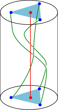
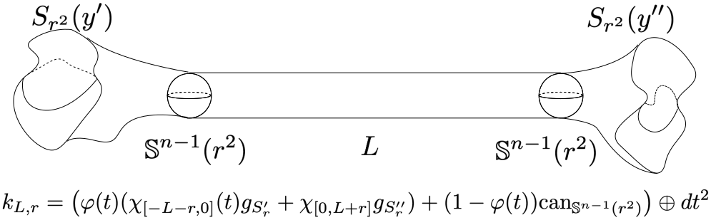
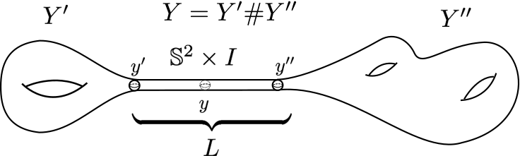
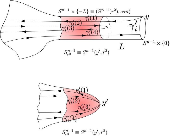
Let $(Y^{\prime},g^{\prime})$, $(Y^{\prime\prime},g^{\prime\prime})$ be two closed, oriented, connected Riemannian $n$-manifolds for $n\geq 3$. We shall now construct a family of metrics on $Y=Y^{\prime}\#Y^{\prime\prime}$. Let us assume to have fixed $y^{\prime}\in Y^{\prime}$, $y^{\prime\prime}\in Y^{\prime\prime}$ and two positive real numbers $L,r>0$ with $r<\frac{1}{2}\cdot\min\{\operatorname{inj}(Y^{\prime},g^{\prime}),\operatorname{inj}(Y^{\prime\prime},g^{\prime\prime})\}$. Excide the geodesic balls of radius $r$ around $y^{\prime}$, $y^{\prime\prime}$ and glue the Riemannian tube $(S^{n-1}\times[-L-r,L+r],k_{L,r})$ to $(Y^{\prime}\smallsetminus B_{g^{\prime}}(y^{\prime},r),g^{\prime})\cup(Y^{\prime}\smallsetminus B_{g^{\prime\prime}}(y^{\prime\prime},r),g^{\prime\prime})$ where $k_{L,r}$ is defined as follows. Let $\varphi:[-L-r,L+r]\rightarrow[0,1]$ be a smooth function which is identically equal to $1$ on an $\frac{r}{3}$-neighbourhood of $\{-L-r,L+r\}$, identically equal to zero on $(-L-\frac{r}{3},L+\frac{r}{3})$, which is non-increasing on $[-L-r,0]$ and non-decreasing on $[0,L+r]$. Then, let us denote by $g_{S_{r}^{\prime}}$ and $g_{S_{r}^{\prime\prime}}$ the restrictions of $g^{\prime}$ and $g^{\prime\prime}$ respectively to $S_{r}(y^{\prime})$ and $S_{r}(y^{\prime\prime})$ (the spheres of radius $r$ centered at $y^{\prime}$, $y^{\prime\prime}$ respectively). We shall define $k_{L,r}$ as follows: < where we denoted by $\chi_{I}$ the characteristic function of the interval $I$ (see Figure 3.1). In the sequel we shall assume to have chosen $r$ such that $\pi r^{2}/2\leq r/3$ or equivalently that $r\leq 2/(3\pi)$. We shall denote by $(Y,g_{L,r})$ the Riemannian manifold which is the result of the gluing, see Figure 3.2.

Figure 3.1: The metric $k_{L,r}$ on the “tube ” of length $R$ connecting the two geodesic balls of radius $r$ $S_{r}(y^{\prime})$ and $S_{r}(y^{\prime\prime})$.

The main result of the next two sections is the following theorem:

Theorem 3.3.

Let $(Y^{\prime},g^{\prime})$ and $(Y^{\prime\prime},g^{\prime})$ be two Riemannian manifolds. Let $L,r>0$ be two positive real constants and $(Y,g_{L,r})$ be the Riemannian manifold constructed as above. There exists a constant $\bar{L}>0$ depending on $(Y^{\prime},g^{\prime})$, $(Y^{\prime\prime},g^{\prime\prime})$ such that for any $L>\bar{L}$ the following holds:

• the critical exponent of the series $\mathcal{P}_{s}(\pi_{1}(Y,y),g_{L,r})$ is smaller than or equal to $\max\{\operatorname{Ent}(Y^{\prime},(g^{\prime})^{\delta}),\operatorname{Ent}(Y^{\prime\prime},(g^{\prime\prime})^{\delta})\}$.

Moreover, chosen $L>\bar{L}$, for every $\varepsilon>0$ there exists an $\bar{r}(L,\varepsilon)$ such that for every $r<\bar{r}(L,\varepsilon)$:

• $|\operatorname{Vol}(Y,g_{L,r})-\operatorname{Vol}(Y^{\prime},g^{\prime})-\operatorname{Vol}(Y^{\prime\prime},g^{\prime\prime})|<\varepsilon$.

Figure 3.2: The Riemannian manifold $(Y,g_{L,r})$ resulting from the gluing.

As a consequence, we have the following estimate which is valid for any dimension $n\geq 3$:

Corollary 3.4.

Let $Y^{\prime}$, $Y^{\prime\prime}$ be two closed, orientable, differentiable $n$-manifolds for $n\geq 3$. Then:

$$\operatorname{MinEnt}(Y^{\prime}\#Y^{\prime\prime})^{3}\leq\operatorname{MinEnt}(Y^{\prime})^{3}+\operatorname{MinEnt}(Y^{\prime\prime})^{3},$$

where $Y^{\prime}\#Y^{\prime\prime}$ denotes the connected sum of $Y^{\prime}$, $Y^{\prime\prime}$.

Proof.

Let $g_{k}^{\prime}$ and $g_{k}^{\prime\prime}$ two sequences of metrics converging to the Minimal Entropy of $Y^{\prime}$ and $Y^{\prime\prime}$ respectively. Up to normalization, we can assume that $\mbox{Ent}(Y^{\prime},g_{k}^{\prime})=\mbox{Ent}(Y^{\prime\prime},g_{k}^{\prime\prime})$; this does not affect the minimality of the sequence. The proof is a straightforward application of Theorem 3.3 to these two sequences of metrics on $Y^{\prime}$, $Y^{\prime\prime}$ minimizing the invariant $\operatorname{EntVol}$. ∎

3.3 The proof of Theorem 3.3

Before proving Theorem 3.3, we shall fix some notation. Denote by $d_{L,r}$ the Riemannian distance associated to $g_{L,r}$. Recall that for any $h\in\pi_{1}(Y,y)$ the value $d_{L,r}(\widetilde{y},h.\widetilde{y})$ does not depend on the lift chosen for $y$. From now on we shall denote by $|h|_{y}$ the length, with respect to the metric $g_{L,r}$ of the shortest geodesic loop representing $h$. Namely, $|h|_{y}=d_{L,r}(\widetilde{y},h.\widetilde{y})$, where $\widetilde{y}$ is any lift of $y$. Similarly, for any choice of $y^{\prime}\in Y^{\prime}$, $y^{\prime\prime}\in Y^{\prime\prime}$ we define $|\cdot|_{y^{\prime}}:\pi_{1}(Y^{\prime},y^{\prime})\longrightarrow\mathbb{R}$ and $|\cdot|_{y^{\prime\prime}}:\pi_{1}(Y^{\prime\prime},y^{\prime\prime})\longrightarrow\mathbb{R}$ the function mapping any class in $\pi_{1}(Y^{\prime},y^{\prime})$, $\pi_{1}(Y^{\prime\prime},y^{\prime\prime})$ into the length of the shortest geodesic representative with respect to $g^{\prime}$, $g^{\prime\prime}$.

Let $y\in Y$ be a point contained in the set $S^{n-1}\times\{0\}$ and $y^{\prime},y^{\prime\prime}$ be the centers of the balls removed from $Y^{\prime},Y^{\prime\prime}$ respectively when constructing the metric $g_{L,r}$. We shall denote by

$$\Phi:\pi_{1}(Y,y)\rightarrow\pi_{1}(Y^{\prime},y^{\prime})\ast\pi_{1}(Y^{\prime\prime},y^{\prime\prime})$$

the isomorphism obtained in two steps:

1. Let $(\widehat{Y},\hat{d}_{L})$ be the metric space obtained as the junction of $(Y^{\prime},g^{\prime})$ and $(Y^{\prime\prime},g^{\prime\prime})$ via an interval $[-L,L]$ (with the standard metric) joining $y^{\prime}$ to $y^{\prime\prime}$. Let $p:(Y,g_{L,r})\rightarrow(\widehat{Y},\hat{d}_{L})$ be the map obtained by collapsing the tube $S^{n-1}\times[-L,L]$ to the interval $[-L,L]$, sending $(S^{n-1}\times[-L-r,-L],g_{L,r})$ onto $B_{g^{\prime}}(y^{\prime},r)$, via the map $S^{n-1}\times\{t\}\mapsto\partial B_{g^{\prime}}(y^{\prime},r)$ and $(S^{n-1}\times[L,L+r],g_{L,r})$ onto $B_{g^{\prime\prime}}(y^{\prime\prime},r)$ via a similar map. Finally $(Y^{\prime}\smallsetminus B_{g^{\prime}}(y^{\prime},r),g_{L,r})$ is sent identically onto itself (and similarly $(Y^{\prime\prime}\smallsetminus B_{g^{\prime\prime}}(r),g_{L,r})$).

2. Call $\hat{y}\in\hat{Y}$ the point $p(S^{n-1}\times\{0\})=p(y)$. By construction we know that $p_{*}:\pi_{1}(Y,y)\rightarrow\pi_{1}(\widehat{Y},\hat{y})$ is an isomorphism. On the other hand it is obviously true that $\pi_{1}(Y^{\prime},y^{\prime})*\pi_{1}(Y^{\prime\prime},y^{\prime\prime})$ is isomorphic to $\pi_{1}(\widehat{Y},\hat{y})$, where the isomorphism is given by the following map: fix $\gamma_{\hat{y},y^{\prime}}$ and $\gamma_{\hat{y},y^{\prime\prime}}$ the unique unit speed geodesics in $(\widehat{Y},\hat{d}_{L})$ joining $\hat{y}$ to $y^{\prime}$ and $y^{\prime\prime}$ respectively. Then, the isomorphism is given by:

   $$g=[\gamma_{1}^{\prime}]\cdot[\gamma_{1}^{\prime\prime}]\cdots[\gamma_{n}^{\prime}]\cdot[\gamma_{n}^{\prime\prime}]\overset{\Psi}{\mapsto}[\gamma_{\hat{y},y^{\prime}}^{-1}*\gamma_{1}^{\prime}*\gamma_{\hat{y},y^{\prime}}]\cdots[\gamma_{\hat{y},y^{\prime\prime}}^{-1}*\gamma_{n}^{\prime\prime}*\gamma_{\hat{y},y^{\prime\prime}}]$$

   for any $g\in\pi_{1}(Y^{\prime},y^{\prime})*\pi_{1}(Y^{\prime\prime},y^{\prime\prime})$.

Hence we define $\Phi=(p_{*})^{-1}\circ\Psi$, and $\Phi^{\prime}:\pi_{1}(Y^{\prime},y^{\prime})\hookrightarrow\pi_{1}(Y,y)$ and $\Phi^{\prime\prime}:\pi_{1}(Y^{\prime\prime},y^{\prime\prime})\hookrightarrow\pi_{1}(Y,y)$ the monomorphisms obtained restricting $\Phi$, which embed $\pi_{1}(Y^{\prime},y^{\prime})$ and $\pi_{1}(Y^{\prime\prime},y^{\prime\prime})$ into $\pi_{1}(Y,y)$. Moreover, we denote by $G_{1}=\Phi^{\prime}\left(\pi_{1}(Y^{\prime},y^{\prime})\right)$ and $G_{2}=\Phi^{\prime\prime}\left(\pi_{1}(Y^{\prime\prime},y^{\prime\prime})\right)$.
By definition of $\pi_{1}(Y^{\prime},y^{\prime})\ast\pi_{1}(Y^{\prime\prime},y^{\prime\prime})$ every $g\in\pi_{1}(Y,y)$ can be (uniquely) written as: $g=h_{1}^{\prime}h_{1}^{\prime\prime}\cdots h_{n}^{\prime}h_{n}^{\prime\prime}$, where $h_{1}^{\prime}$ and $h_{n}^{\prime\prime}$ are possibly equal to the identity, $h_{i}^{\prime}\in\pi_{1}(Y^{\prime},y^{\prime})\smallsetminus\{\operatorname{id}\}$ for $i=2,\dots,n$ and $h^{\prime\prime}_{i}\in\pi_{1}(Y^{\prime\prime},y^{\prime\prime})\smallsetminus\{\operatorname{id}\}$ for $i=1,\dots,n-1$. Notice that we are making a little abuse of notation since we are omitting the identification of the elements of $\pi_{1}(Y^{\prime},y^{\prime})$ and $\pi_{1}(Y^{\prime\prime},y^{\prime\prime})$ with the elements of $\pi_{1}(Y,y)$ which correspond via the isomorphisms $\Phi^{\prime}$, $\Phi^{\prime\prime}$.

Lemma 3.5.

With the above notation, assume $L\geq\frac{\pi r}{2}$. For any element $g\in\pi_{1}(Y,y)$ let $g=h_{1}^{\prime}h_{1}^{\prime\prime}\dots h_{n}^{\prime}h_{n}^{\prime\prime}$ be a reduced syllabic form for $g$. Then:

$$\lvert g\rvert_{y}\geq\sum_{i=1}^{n}(|h_{i}^{\prime}|_{y^{\prime}}+2L)+\sum_{i=1}^{n}(|h_{i}^{\prime\prime}|_{y^{\prime\prime}}+2L)$$

Proof.

First of all we observe that by construction of the metric the sets $S^{n-1}\times\{t\}$ where $t\in[-L-\frac{r}{3},L+\frac{r}{3}]$ are totally geodesic hypersurfaces (because the metric is a Riemannian product). Moreover the set $S^{n-1}\times\{t\}$ for $t\in[-L,L]$ is such that every minimizing geodesic $\alpha_{PQ}$ joining pair of points $P$, $Q\in S^{n-1}\times\{t\}$ is entirely contained in $\subset S^{n-1}\times\{t\}$. Indeed, any curve $\beta_{PQ}$ joining the two points and contained in the tube $(S^{n-1}\times[-L-\frac{r}{3},L+\frac{r}{3}],k_{L,r})$ has length greater than or equal to the length of its projection on $S^{n-1}\times\{t\}$ with equality holding only for those curves contained into $S^{n-1}\times\{t\}$, because the metric in the tube is a Riemannian product. Furthermore, since $r\leq 2/(3\pi)$, every curve joining $P$ and $Q$ and escaping the tube $(S^{n-1}\times[-L-\frac{r}{3},L+\frac{r}{3}],k_{L,r})$ has length greater than $\pi r$, which is equal to the diameter of $(S^{n-1}\times\{t\},k_{L,r}|_{S^{n-1}\times\{t\}})$. Let $\gamma$ be a shortest representative in the homotopy class of $g$. Denote by $\gamma_{i}^{\prime},\gamma_{i}^{\prime\prime}$ the connected subsegments of $\gamma$ entirely contained in one of the two sides separated by $S^{n-1}\times\{0\}$. Observe that:

$$|\{\gamma_{i}^{\prime}\}|=|\{h_{i}^{\prime}\,:\,h_{i}^{\prime}\neq 1\}|,\quad|\{\gamma_{i}^{\prime\prime}\}|=|\{h_{i}^{\prime\prime}\,:\,h_{i}^{\prime\prime}\neq 1\}|$$ (3.1)

Indeed, for any $i=1,...,m$ and any $j=1,...,k$ consider two minimizing geodesics $\xi_{i}^{\prime}$, $\xi_{j}^{\prime\prime}$ contained in $S^{n-1}\times\{0\}$ and connecting $y$ respectively to $\gamma_{i}^{\prime}(0)$ and to $\gamma_{j}^{\prime\prime}(0)$ and call $\tilde{\gamma}_{i}^{\prime}$ ($\tilde{\gamma}_{j}^{\prime\prime}$ respectively) the path obtained by joining $\gamma_{i}^{\prime}$ to the $g_{L,r}$-geodesic connecting $\gamma_{i}^{\prime}(1)$ to $\gamma_{i}^{\prime}(0)$. By construction the loop $\gamma$ is homotopic to the join of the loops $[(\xi_{i}^{\prime})^{-1}*\tilde{\gamma}_{i}^{\prime}*\xi_{i}^{\prime}]$’s and $[(\xi_{j}^{\prime\prime})^{-1}*\tilde{\gamma}_{j}^{\prime\prime}*\xi_{j}^{\prime\prime}]$’s following the order in which the $\gamma_{i}^{\prime}$’s, $\gamma_{j}^{\prime\prime}$’s appear along $\gamma$. Notice that by construction the $\gamma_{i}^{\prime}$’s and the $\gamma_{j}^{\prime\prime}$’s appear alternately. Let $p:Y\rightarrow\widehat{Y}$ be the map defined before and let

$$\Phi^{-1}=\Psi^{-1}\circ p_{*}:\pi_{1}(Y,y)\rightarrow\pi_{1}(Y^{\prime},y^{\prime})*\pi_{1}(Y^{\prime\prime},y^{\prime\prime})$$

be the inverse of the isomorphism constructed before the Lemma. Then,

$$\Phi^{-1}([(\xi_{i}^{\prime})^{-1}*\tilde{\gamma}_{i}^{\prime}*\xi_{i}^{\prime}])\in\pi_{1}(Y^{\prime},y^{\prime})\smallsetminus\{1\}\mbox{ and }\Phi^{-1}([(\xi_{j}^{\prime\prime})^{-1}*\tilde{\gamma}_{j}^{\prime\prime}*\xi_{j}^{\prime\prime}])\in\pi_{1}(Y^{\prime\prime},y^{\prime\prime})\smallsetminus\{1\}.$$

Otherwise, if $\Phi^{-1}([(\xi_{i}^{\prime})^{-1}*\tilde{\gamma}_{i}^{\prime}*\xi_{i}^{\prime}])\in\pi_{1}(Y^{\prime},y^{\prime})\smallsetminus\{1\}$ were not trivial, we could replace $\gamma_{i}^{\prime}$ with a minimizing geodesic $\delta_{i}^{\prime}$ (contained in $S^{n-1}\times\{0\}$) connecting the two endpoints of $\gamma_{i}^{\prime}$, thus obtaining a shortest representative of $\gamma$, thus contradicting the minimality of $\gamma$.
As a consequence $|\{\gamma_{i}^{\prime}\}|=|\{h_{i}^{\prime}\,:\,h_{i}^{\prime}\neq 1\}|$ and $|\{\gamma_{j}^{\prime\prime}\}|=|\{h_{j}^{\prime\prime}\,:\,h_{j}^{\prime\prime}\neq 1\}|$. Moreover, by the previous discussion:

$$g=\Phi^{-1}[\xi_{1}^{\prime-1}*\tilde{\gamma}_{1}^{\prime}*\xi_{1}^{\prime}]\cdot\Phi^{-1}[\xi_{1}^{\prime\prime-1}*\tilde{\gamma}_{1}^{\prime\prime}*\xi_{1}^{\prime\prime}]\cdots\Phi^{-1}[\xi_{n}^{\prime-1}*\tilde{\gamma}_{n}^{\prime}*\xi_{n}^{\prime}]\cdot\Phi^{-1}[\xi_{n}^{\prime\prime-1}*\tilde{\gamma}_{n}^{\prime\prime}*\xi_{n}^{\prime\prime}]$$

By the unicity of the reduced form of an element in a free product we deduce that: $\Phi^{-1}([(\xi_{i}^{\prime})^{-1}*\tilde{\gamma}_{i}^{\prime}*\xi_{i}])=h_{i}^{\prime}$, $\Phi^{-1}([(\xi_{j}^{\prime\prime})^{-1}*\tilde{\gamma}_{j}^{\prime\prime}*\xi_{j}^{\prime\prime}])=h_{j}^{\prime\prime}$ for every $i,j=1,\dots n$.
Recall that our goal is to provide a sufficiently accurate estimate from below to the length of the shortest representative $\gamma$ of $g$ with respect to the Riemannian metric $g_{L,r}$ in terms of $L,r$ and of the lengths of the shortest representatives (with respect to the metrics $g^{\prime}$, $g^{\prime\prime}$) of the elements $h_{i}^{\prime}$’s, $h_{j}^{\prime\prime}$’s of $\pi_{1}(Y^{\prime},y^{\prime})$ and $\pi_{1}(Y^{\prime\prime},y^{\prime\prime})$ for every $i,j=1\dots,n$.

Claim (0). Any $\gamma_{i}^{\prime}$ (respectively $\gamma_{j}^{\prime\prime}$) is such that $|\gamma_{i}^{\prime-1}(S^{n-1}\times\{t\})|<+\infty$ for any $t\in(-L,L)$ (respectively, $|\gamma_{j}^{\prime\prime-1}(S^{n-1}\times\{t\})|<+\infty$ for any $t\in(-L,L)$).

Proof of Claim (0). Straightforward from the definition of the metric. ∎

Claim (1). Any $\gamma_{i}^{\prime}$ (respectively $\gamma_{j}^{\prime\prime}$) is such that $|\gamma_{i}^{\prime-1}(S^{n-1}\times\{t\})|=2$ for any $t\in(-L,0]$ (respectively, $|\gamma_{j}^{\prime\prime-1}(S^{n-1}\times\{t\})|=2$ for any $t\in[0,L)$).

Proof of Claim (1). Let us observe first that $|\gamma_{i}^{\prime-1}(S^{n-1}\times\{t\})|\geq 2$ for every $t\in[-L,0]$. Otherwise the loop $\xi_{i}^{\prime-1}*\tilde{\gamma}_{i}^{\prime}*\xi_{i}^{\prime}$ would be trivial, which is not. On the other hand assume that $\gamma_{i}^{\prime}$ crosses a sphere $S^{n-1}\times\{t\}$, with $t\in(-L,0]$, for at least three times. Then, we would have that $|\gamma_{i}^{\prime-1}(S^{n-1}\times\{-L\})|\geq 4$. Now, let $s_{2}$ and $s_{2k-1}$ be respectively the first time in which $\gamma_{i}^{\prime}$ crosses $S^{n-1}\times\{-L\}$ in direction $S^{n-1}\times\{0\}$ and the last time in which $\gamma_{i}^{\prime}$ crosses $S^{2}\times\{-L\}$ in direction $Y^{\prime}$. Connect $\gamma_{i}^{\prime}(s_{2})$ with $\gamma_{i}^{\prime}(s_{2k-1})$ with a geodesic segment in $(S^{n-1}\times\{-L\},g_{L,r}|_{S^{n-1}\times\{-L\}})$, call it $\zeta_{i}^{\prime}$. Then the path $\gamma_{i}^{\prime}|_{[0,s_{2}]}*\zeta_{i}^{\prime}*\gamma_{i}^{\prime}|_{[s_{2k-1},1]}$ is homotopic with fixed ends to $\gamma_{i}^{\prime}$, and is shorter. This is a contradiction because substituting $\gamma_{i}^{\prime}$ with this new path would produce a shorter representative for $g$.∎

We shall now look at the path $\gamma_{i}^{\prime}$ outside the tube $S^{n-1}\times(-L,0]$ (respectively, $S^{n-1}\times[0,L)$). Let $\gamma_{i}^{\prime}(1)=\gamma_{i}^{\prime}|_{I_{1}}$,…, $\gamma_{i}^{\prime}(k_{i})=\gamma_{i}^{\prime}|_{I_{k_{i}}}$ be the subpaths of $\gamma_{i}^{\prime}$ contained in $(S^{n-1}\times[-r-L,-L],g_{L,r}|_{S^{n-1}\times[-r-L,-L]})$. Now, look at $p(\gamma_{i}^{\prime})$ in restriction to $Y^{\prime}$ and observe that it is a loop based at $y^{\prime}$. Moreover, its homotopy class $[p(\gamma_{i}^{\prime})|_{Y^{\prime}}]=h_{i}^{\prime}$. Now, let $\eta_{i}^{\prime}(j)=p(\gamma_{i}^{\prime}(j))$. The following hold:

$$\ell_{g_{L,r}}(\gamma_{i}^{\prime}(j))\geq\ell_{quot}(\eta_{i}^{\prime}(j))\geq r=\ell_{g^{\prime}}(\zeta_{i}^{\prime}(j)))$$

where we denoted by $\ell_{quot}$ the quotient metric of $(S^{n-1}\times[-L-r,-L],g_{L,r})/\sim$ where $(x,t)\sim(y,t^{\prime})$ if and only if $t=t^{\prime}=-L$; and where we introduced the notation $\zeta_{i}^{\prime}$ for the $g^{\prime}$-geodesic segment joining $y^{\prime}=\eta_{i}^{\prime}(j)(0)$ to the other endpoint $\eta_{i}^{\prime}(j)(1)$ (see Figure 3.3).

Figure 3.3: The projection $p:(Y,g_{L,r})\rightarrow(\widehat{Y},\hat{d}_{L})$, and the images $\eta_{i}^{\prime}(j)=p(\gamma_{i}^{\prime})$.

Since we are in balls of radius shorter than the injectivity radius of $(Y^{\prime},g^{\prime})$, $\eta_{i}^{\prime}(j)$ is homotopic with fixed endpoints to $\zeta_{i}^{\prime}(j)$. On the other hand, observe that $p$ in restriction to $(Y^{\prime}\smallsetminus B_{g^{\prime}}(y^{\prime},r),g_{L,r})$ is an isometry on its image. Hence, the path obtained from $p(\gamma_{i}^{\prime})|_{Y^{\prime}}$ replacing the $\eta_{i}^{\prime}(j)$ with the $\zeta_{i}^{\prime}(j)$ is a representative of the same homotopy class and its length is less than the length of $p(\gamma_{i}^{\prime})|_{Y^{\prime}}$. We deduce the following inequality:

$$\ell_{g_{L,r}}(\gamma_{i}^{\prime})\geq|h_{i}^{\prime}|_{y^{\prime}}+2d_{g_{L,r}}(S^{n-1}\times\{-L\},S^{n-1}\times\{0\})=|h_{i}^{\prime}|_{y^{\prime}}+2L$$

which is the desired estimate. ∎

Now we can prove Theorem 3.3

Proof of Theorem 3.3.

Let $g=g_{1}^{\prime}g_{1}^{\prime\prime}\cdots g_{n}^{\prime}g_{n}^{\prime\prime}\in\pi_{1}(Y,y)$, where $g_{i}^{\prime}=\Phi^{\prime}(h_{i}^{\prime})$, $g_{i}^{\prime\prime}\in\Phi^{\prime\prime}(h_{i}^{\prime\prime})$, $h_{i}^{\prime}\in\pi_{1}(Y^{\prime},y^{\prime})$ and $h_{i}^{\prime\prime}\in\pi_{1}(Y^{\prime\prime},y^{\prime\prime})$, with possibly $h_{1}^{\prime}=1$, $h_{n}^{\prime\prime}=1$. Then, by Lemma 3.5 we have:

$$\lvert g\rvert_{y}\geq\sum_{i=1}^{n}\left(\lvert h_{i}^{\prime}\rvert_{y^{\prime}}+\lvert h_{i}^{\prime\prime}\rvert_{y^{\prime\prime}}\right)+4nL$$

Thus we get:

$$e^{-s\lvert g\rvert_{y}}\leq e^{-4nL}\cdot e^{-s\lvert h_{1}^{\prime}\rvert_{y^{\prime}}}\cdots e^{-s\lvert h_{n}^{\prime}\rvert_{y^{\prime}}}\cdot e^{-s\lvert h_{1}^{\prime\prime}\rvert_{y^{\prime\prime}}}\cdots e^{-s\lvert h_{n}^{\prime\prime}\rvert_{y^{\prime\prime}}}$$

So the Poincaré series of $\pi_{1}(Y,y_{0})$ with respect to the metric $g_{L,r}^{\delta}$ can be estimated as follows:

$$\mathcal{P}\left(\pi_{1}(Y,y),g_{L,r}\right)=\sum_{g\in\pi_{1}(Y,y)}e^{-s|g|_{y}}\leq$$

$$\leq 1+\sum_{\mathclap{\begin{subarray}{c}n\geq 1\\ h_{i}^{\prime}\in(\pi_{1}(Y^{\prime},y^{\prime}))^{\ast}\\ h_{i}^{\prime\prime}\in(\pi_{1}(Y^{\prime\prime},y^{\prime\prime}))^{\ast}\end{subarray}}}\left(e^{-s|h_{1}^{\prime}\cdots h_{n}^{\prime}h_{n}^{\prime\prime}|_{y}}+e^{-s|h_{1}^{\prime}\cdots h_{n-1}^{\prime\prime}h_{n}^{\prime}|_{y}}+e^{-s|h_{1}^{\prime\prime}h_{2}^{\prime}\cdots h_{n}^{\prime\prime}|_{y}}+e^{-s|h_{1}^{\prime\prime}h_{2}^{\prime}\cdots h_{n-1}^{\prime\prime}h_{n}^{\prime}|_{y}}\right){\leq}$$

$${\leq}1+4\cdot\sum_{n\geq 1}\left(\sum_{h^{\prime}\in(\pi_{1}(Y^{\prime},y^{\prime}))^{\ast}}e^{-s|h^{\prime}|_{y}}\right)^{n}\left(\sum_{h^{\prime\prime}\in(\pi_{1}(Y^{\prime\prime},y^{\prime\prime}))^{\ast}}e^{-s|h^{\prime\prime}|_{y}}\right)^{n}{\leq}$$

$${\leq}1+4\sum_{n\geq 1}\left(e^{-s2L}\sum_{\mathclap{h^{\prime}\in(\pi_{1}(Y^{\prime},y^{\prime}))^{\ast}}}e^{-s|h^{\prime}|_{y^{\prime}}}\right)^{n}\left(e^{-s2L}\sum_{\mathclap{h^{\prime\prime}\in(\pi_{1}(Y^{\prime\prime},y^{\prime\prime}))^{\ast}}}e^{-s|h^{\prime\prime}|_{y^{\prime\prime}}}\right)^{n}{\leq}$$

$${\leq}1+4\sum_{n\geq 1}\left(e^{-4sL}\cdot\mathcal{P}^{\ast}_{s}(\pi_{1}(Y^{\prime},y^{\prime}),g^{\prime})\cdot\mathcal{P}^{\ast}_{s}(\pi_{1}(Y^{\prime\prime},y^{\prime\prime}),g^{\prime\prime})\right)^{n}$$

where the second inequality is consequence of a rearrangement of the summands, the third follows from Lemma 3.5 and the last follows from the definition of the Poincaré series, with $\mathcal{P}^{\ast}$ denoting the Poincaré series without the summand corresponding to the identity.
Now for any arbitrarily chosen

$$s>s_{Y^{\prime},Y^{\prime\prime}}=\max\{\operatorname{Ent}(Y^{\prime},g^{\prime}),\operatorname{Ent}(Y^{\prime\prime},g^{\prime\prime})\}$$

the series $\mathcal{P}_{s}^{*}(\pi_{1}(Y^{\prime},y^{\prime}),g^{\prime})$ and $\mathcal{P}_{s}^{*}(\pi_{1}(Y^{\prime\prime},y^{\prime\prime}),g^{\prime\prime})$ converge to $P_{1}$, $P_{2}$. Thus the problem of the convergence of $\mathcal{P}_{s}(\pi_{1}(Y,y),g_{L,r})$ is reduced to the convergence of the geometric series:

$$\sum_{\mathclap{n\geq 1}}\left(e^{-s4L}\cdot P_{1}\cdot P_{2}\right)^{n}$$

This series converges if the length $L$ of the interpolation cylinder is large enough:

$$L>\frac{\log(P_{1}\cdot P_{2})}{4s_{Y^{\prime},Y^{\prime\prime}}}$$

As $s>s_{Y^{\prime},Y^{\prime\prime}}=\max\{\operatorname{Ent}(Y^{\prime},g^{\prime}),\operatorname{Ent}(Y^{\prime\prime},g^{\prime\prime})\}$ this shows that the critical exponent of $\mathcal{P}(\pi_{1}(Y,y),g_{L,r})$ is less or equal to $s_{Y^{\prime},Y^{\prime\prime}}$ for $L$ sufficiently large. This concludes the proof of Theorem 3.3 (1).

Let us now focus on assertion (2), i.e. the convergence of the volume. By construction of the metric $g_{L,r}$ we have:

$$\operatorname{Vol}(Y^{\prime}\smallsetminus B_{g^{\prime}}(y^{\prime},r),g^{\prime})+\operatorname{Vol}(Y^{\prime\prime}\smallsetminus B_{g^{\prime\prime}}(y^{\prime\prime},r),g^{\prime\prime})\leq\operatorname{Vol}(Y,g_{L,r})$$

but also:

$$\operatorname{Vol}(Y,g_{L,r})=\operatorname{Vol}(Y^{\prime}\smallsetminus B_{g^{\prime}}(y^{\prime},r),g^{\prime})+\operatorname{Vol}(Y^{\prime\prime}\smallsetminus B_{g^{\prime\prime}}(y^{\prime\prime},r),g^{\prime\prime})+V(L,r)$$

where:

$$V(L,r)=(S^{n-1}\times[-L-r,L+r],g_{L,r}|_{S^{n-1}\times[-L-r,L+r]})$$

Now observe that in restriction to $S^{n-1}\times[-L-r,L+r]$ the metric $g_{L,r}$ is equal to the metric $k_{L,r}$ described in Chapter 4, §3.2. Moreover, denoting:

$$A^{\prime}=\max_{r\in[0,\frac{\operatorname{inj}(y^{\prime})}{2}]}\{\mathcal{A}_{g^{\prime}}(S_{r}^{\prime}(y^{\prime}))\}$$

and

$$A^{\prime\prime}=\max_{r\in[0,\frac{\operatorname{inj}(y^{\prime\prime})}{2}]}\{\mathcal{A}_{g^{\prime\prime}}(S_{r}^{\prime\prime}(y^{\prime\prime}))\}$$

we observe that these are finite quantities. Call $A=\max\{A^{\prime},A^{\prime\prime}\}$; then

$$V(L,r)\leq A\cdot 2r+(\omega_{n-1}r^{n-1})\cdot(2L+2r),$$

where $\omega_{n-1}=\mathcal{A}(\mathbb{S}^{n-1})$. Hence, for every fixed $L>\bar{L}$ and every $\varepsilon>0$ there exists $\bar{r}(L,\varepsilon)>0$ such that for every $r<\bar{r}(L,\varepsilon)$ we have:

$$|\operatorname{Vol}(Y,g_{L,r})-\operatorname{Vol}(Y^{\prime},g^{\prime})-\operatorname{Vol}(Y^{\prime\prime},g^{\prime\prime})|<\varepsilon$$

which proves part (2). ∎

3.4 Proof of Theorem 3.1

Before going into the proof of Theorem 3.1 we recall some facts:

1. Let $X$ be a closed, orientable Seifert fibred manifold or a graph-manifold, then we have $\operatorname{MinEnt}(X)=0$ by [AP03].

2. Let $X$ be a closed, orientable manifold which admits a hyperbolic metric. Then by [BCG95] we know that the hyperbolic metric realizes the Minimal Entropy, that is $\operatorname{MinEnt}(X)=2\cdot\left(\operatorname{Vol}(X,hyp)\right)^{1/3}$.

3. Finally from Theorem LABEL:thm_construction_sequence_on_irreducible_Y we know that on every irreducible, closed, orientable $3$-manifold with non-trivial $JSJ$ decomposition and at least one hyperbolic $JSJ$ component we have

   $$\operatorname{MinEnt}(X)=2\left(\sum_{i=1}^{k}\operatorname{Vol}(int(X_{i}),hyp_{i})\right)^{1/3}$$

   i.e., $\operatorname{MinEnt}(Y)^{3}$ is additive with respect to the connected sum.

Proof of Theorem 3.1.

The theorem follows by iteratively applying Corollary 3.4 to the prime summands of the manifold $Y$, keeping into account the estimates (1)—(3) existing for the Minimal Entropy of the prime summands. ∎

Chapter 4 The lower bound via the barycentre method:
irreducible $3$-manifolds

In this Chapter we shall find the optimal lower bound for the Minimal Entropy of a closed, orientable, irreducible $3$-manifold $Y$. We shall handle the reducible case in Chapter 6.

Let $Y$ be a closed, orientable, irreducible $3$-manifold, consider its $JSJ$ decomposition and denote by $X_{1},\dots,X_{n}$ the hyperbolic $JSJ$ components. For every $i=1,\dots,n$ the manifold $int(X_{i})$ can be endowed with a complete hyperbolic, finite volume metric, unique up to isometries by Mostow Rigidity Theorem; we shall denote it by $hyp_{i}$.

The main result of this section is the following.

Theorem 4.1.

Let $Y$ be a closed, orientable, irreducible $3$-manifold, and let $X_{1},\dots X_{k}$ be its hyperbolic $JSJ$ components. Then, the following inequality holds:

$$\operatorname{MinEnt}(Y)\geq 2\cdot\left(\sum_{i=1}^{k}\operatorname{Vol}(int(X_{i}),hyp_{i})\right)^{1/3}.$$

The last statement, together with Theorem LABEL:thm_construction_sequence_on_irreducible_Y gives the exact computation of the minimal entropy in the irreducible case. In order to prove this inequality, we shall use the barycenter method applied to a $1$-parameter family of $C^{2}$ Riemannian metrics $\{g_{\delta}\}$ on $Y$, which are non-positively curved and locally isometric to $\mathbb{H}^{3}$ on larger and larger open subsets (as $\delta\rightarrow 0$), constructed in Chapter LABEL:section_a_conjectural_minimizing_sequence_irreducible.

4.1 The barycentre method

In this section we shall give a brief introduction to the barycenter method. Roughly speaking, given a map $f:(Y,g)\longrightarrow(X,g_{0})$ which lifts to a $\lambda$-equivariant map $\widetilde{f}:(\widetilde{Y},\tilde{g})\longrightarrow(\widetilde{X},\tilde{g}_{0})$ between the universal covers —here $\lambda=f_{*}:\pi_{1}(Y)\rightarrow\pi_{1}(X)$ is the homomorphism induced by $f$ between the first homotopy groups—, the method consists in:

• Immersing $(\widetilde{Y},\tilde{g})$ in $\mathcal{M}(Y,g)$ —the space of positive and finite Borel measures on $(\widetilde{Y},\tilde{g})$— via a family of $\pi_{1}(Y)$-equivariant maps $y\mapsto\mu_{c,y}$.

• Taking $\widetilde{f}_{\ast}(\mu_{c,y})\in\mathcal{M}(X,g_{0})$, the push-forward measure with respect to $\widetilde{f}$.

• Projecting from $\mathcal{M}(X,g_{0})$ on $(\widetilde{X},\tilde{g}_{0})$ by composing with the map which associates to any measure in $\mathcal{M}(X,g_{0})$ its barycenter, that we are going to describe in detail in few lines.

This way, we shall obtain, via the composition of the three maps described above, a family of maps $\widetilde{F}_{c}:\widetilde{Y}\longrightarrow\widetilde{X}$ —namely, $\widetilde{F}_{c}(y)=\operatorname{bar}[\widetilde{f}_{\ast}\mu_{c,y}]$:

By construction, the maps $\widetilde{F}_{c}$ have the following properties:

• $\widetilde{F}_{c}$ is $\lambda$-equivariant, i.e. $\widetilde{F}_{c}(h.\tilde{y})=\lambda(h).\widetilde{F}_{c}(\tilde{y})$; hence, every $\widetilde{F}_{c}$ induces a quotient map $F_{c}:Y\rightarrow X$ such that $(F_{c})_{*}=\lambda$;

• the induced maps $F_{c}$ are homotopic to the map $f$ for every $c$;

In our context, we shall consider the following family of immersions in the space $\mathcal{M}(Y,g)$:

$$y\mapsto d\mu_{c,y}(y^{\prime}):=e^{-c\tilde{d}(y,y^{\prime})}dv_{\tilde{g}}(y^{\prime}).$$

where $dv_{\tilde{g}}$ is the Riemannian measure of the metric $\tilde{g}$ on $\widetilde{Y}$ and $c>\operatorname{Ent}(g)$. All these measures are finite by the integral characterization of the entropy in the compact case, see Section 3.1.

Now we shall give the formal definition of the barycentre of a measure $\mu$ on a complete, simply connected Riemannian manifold having non-positive curvature. For the proof of the good definition of the barycenter, and of the useful properties provided in Lemmata 4.4, 4.6, 4.7 we refer to [Sam99].

Definition 4.2.

Let $(\widetilde{X},\tilde{g}_{0})$ be a complete simply connected Riemannian manifold with non-positive curvature, and $\mu\in\mathcal{M}(\widetilde{X},\tilde{g}_{0})$ a positive, finite Borel measure on it. If there exists at least a point $x_{0}\in\widetilde{X}$ such that the integral $\int_{\widetilde{X}}\tilde{d}_{0}(x_{0},x^{\prime})^{2}d\mu(x^{\prime})$ converges, then the so-called Leibniz function:

$$B_{\mu}(x)=\int_{\widetilde{X}}\tilde{d}_{0}(x^{\prime},x)^{2}d\mu(x^{\prime})$$

is well defined for any $x\in\widetilde{X}$ —namely, the integral converges for any $x\in\widetilde{X}$—, is positive and is $C^{\infty}$.

As a consequence of the strict convexity of the Riemannian distance function $d_{0}$ on $\widetilde{X}$, it follows that the Leibniz function associated to any $\mu\in\mathcal{M}(\widetilde{X},\tilde{g}_{0})$ is a strictly convex function. Moreover, for any fixed $x_{0}$ we have that $|B_{\mu}(x)-B_{\mu}(x_{0})|\rightarrow\infty$ as $\tilde{d}_{0}(x,x_{0})\rightarrow\infty$. We refer to [Sam99] for these facts. As a consequence, it follows that $B_{\mu}$ admits a unique critical point. It makes thus sense to give the following definition.

Definition 4.3.

Let $(\widetilde{X},\tilde{g}_{0})$ and $\mu$ as above. We define the barycentre of $\mu$ as the unique critical point of the associated Leibniz function. In particular, in this setting the critical point is a minimum. It will be denoted $\operatorname{bar}[\mu]$. The barycenter is equivariant, i.e., for every $\sigma\in\operatorname{Isom}(\widetilde{X},\tilde{g}_{0})$ we have $\operatorname{bar}[\sigma_{\ast}\mu]=\sigma.\operatorname{bar}[\mu]$.

We shall now list some properties verified by the maps $\widetilde{F}_{c}$, $F_{c}$. These properties are classical (see for example [Sam99]), nevertheless we shall provide proofs for the sake of completeness.

Lemma 4.4 (Equivariance of $\widetilde{F}_{c}$).

Using the notation introduced above, the maps $\widetilde{F}_{c}:\widetilde{Y}\longrightarrow\widetilde{X}$ are $\lambda$-equivariant, and thus induce maps between the quotients $F_{c}:Y\longrightarrow X$.

Proof.

We recall that $\lambda=f_{*}:\pi_{1}(Y)\longrightarrow\pi_{1}(X)$ is the homomorphism induced by $F:Y\rightarrow X$. We need to prove that the $\widetilde{F}_{c}$ are $\lambda$-equivariant, i.e., $\operatorname{bar}[\tilde{f}_{\ast}\mu_{c,h.y}]=\lambda(h).\operatorname{bar}[\tilde{F}_{\ast}\mu_{c,y}]$ for any $h\in\pi_{1}(Y)$. This will follow from:

$$B_{\mu_{c,h.y}}(\lambda(h).x)=B_{\mu_{c,y}}(x)$$

Indeed, the following equalities hold:

$$B_{\mu_{c,h.y}}(\lambda(h).x)=\int_{\widetilde{X}}\tilde{d}_{0}\left(z,\lambda(h).x\right)^{2}d(\tilde{f}_{*}\mu_{c,h.y})(z)=$$

$$=\int_{\widetilde{Y}}\tilde{d}_{0}\left(\tilde{f}(y^{\prime}),\lambda(h).x\right)^{2}\mu_{c,h.y}(y^{\prime})=$$

$$=\int_{\widetilde{Y}}\tilde{d}_{0}\left(\tilde{f}(y^{\prime}),\lambda(h).x\right)^{2}e^{-c\tilde{d}(h.y,y^{\prime})}dv_{\tilde{g}}(y^{\prime})=$$

$$=\int_{\widetilde{Y}}\tilde{d}_{0}\left(\lambda(h).\tilde{f}(y^{\prime\prime}),\lambda(h).x\right)^{2}e^{-c\tilde{d}(h.y,h.y^{\prime\prime})}dv_{\tilde{g}}(h.y^{\prime\prime})=$$

$$=\int_{\widetilde{Y}}\tilde{d}_{0}\left(\tilde{f}(y^{\prime\prime}),x\right)^{2}e^{-c\tilde{d}(y,y^{\prime\prime})}dv_{\tilde{g}}(y^{\prime\prime})=B_{\mu_{c,y}}(x)$$

Hence, the minimum of $B_{\mu_{c,h.y}}$ is equal to the image via $\lambda(h)$ of the minimum of $B_{\mu_{c,y}}$. ∎

Lemma 4.5.

The maps $F_{c}:Y\longrightarrow X$ are homotopic to $f$.

Proof.

Since $(X,g_{0})$ is non-positively curved we know that $X$ is an aspherical space. Hence, the set of homotopy classes of maps $[Y,X]$ from $Y$ to $X$ is in bijection with $\mathrm{Hom}(\pi_{1}(Y),\pi_{1}(X))/\mathrm{Inn}(\pi_{1}(X))$. As a consequence of this bijection, and of the fact that $\lambda=f_{*}=(F_{c})_{*}:\pi_{1}(Y)\rightarrow\pi_{1}(X)$ we deduce that $F_{c}$ is homotopic to $f$. ∎

By taking derivatives of the Leibniz function it is easily seen that for every complete, simply connected, non-positively curved $(\widetilde{X},\tilde{g}_{0})$ and every positive, finite Borel measure $\mu$ on $(\widetilde{X},\tilde{g}_{0})$ the barycenter $\operatorname{bar}[\mu]$ is uniquely determined by the implicit equation: $\forall v\in T_{\operatorname{bar}[\mu]}\widetilde{X}$,

$$(dB_{\mu})_{\operatorname{bar}[\mu]}(v)=2\int_{\widetilde{X}}(\tilde{\rho}_{0})_{x^{\prime}}(\operatorname{bar}[\mu])\cdot(d(\tilde{\rho}_{0})_{x^{\prime}})_{\operatorname{bar}[\mu]}(v)d\mu(x^{\prime})=0,$$ (4.1)

where $(\tilde{\rho}_{0})_{x^{\prime}}(\cdot)=\tilde{d}_{0}(x^{\prime},\cdot)$. As a consequence, we have the following implicit equations for the maps $\widetilde{F}_{c}$ (see [Sam99] or [Sam98] for a detailed proof of the following Lemmata 4.6, 4.7 and 4.8):

Lemma 4.6 (Implicit equations for $\widetilde{F}_{c}$).

The functions $\widetilde{F}_{c}$ are univocally determined by the vectorial implicit equations $G_{c}(\widetilde{F}_{c}(y),y)=0$, where $G_{c}=(G_{c}^{i}):\widetilde{X}\times\widetilde{Y}\longrightarrow\mathbb{R}^{n}$ is defined as

$$G_{c}^{i}(x,y)=\frac{1}{2}\int_{\widetilde{Y}}d_{x}[(\tilde{\rho}_{0})_{\tilde{f}(y^{\prime})}]^{2}(E_{i})\,e^{-c\tilde{d}(y,y^{\prime})}dv_{\tilde{g}}(y^{\prime}),$$

where $\{E_{i}\}_{i=1}^{n}$ is a $\tilde{g}_{0}$-orthonormal basis for the tangent space $T_{x}\widetilde{X}$, and $(\tilde{\rho}_{0})_{\tilde{f}(y^{\prime})}(\cdot)=\tilde{d}_{0}(\tilde{f}(y^{\prime}),\cdot)$.

Proof.

Since $(\widetilde{X},\tilde{g}_{0})$ is non-positively curved, the Riemannian universal cover $\widetilde{X}$ is diffeomorphic to $\mathbb{R}^{n}$; in particular, it has trivial tangent bundle. By the definition of the barycentre, $\widetilde{F}_{c}(y)=\operatorname{bar}[f_{\ast}\mu_{c,y}]$ is the unique point of $\widetilde{X}$ satisfying, for every $i=1,\dots,n$:

$$0=\left(dB_{\mu_{c,y}}\right)_{\widetilde{F}_{c}(y)}(E_{i})=\left(d\int_{\widetilde{X}}(\tilde{\rho}_{0})_{x^{\prime}}(x)^{2}\widetilde{f}_{\ast}\mu_{c,y}(x^{\prime})\right)_{\widetilde{F}_{c}(y)}(E_{i})=$$

$$=\int_{\widetilde{Y}}\left(d[(\tilde{\rho}_{0})_{\widetilde{f}(z)}]^{2}\right)_{\widetilde{F}_{c}(y)}(E_{i})e^{-\left(c\tilde{d}(y,z)\right)}dv_{\tilde{g}}(z)=2G_{c}^{i}(\widetilde{F}_{c}(y),y)$$

where we were allowed to pass the derivative through the integral sign thanks to Lebesgue Dominated Convergence Theorem. Indeed, if $x(t)\rightarrow x$, then the following estimates hold:

$$\left\lvert\frac{\tilde{d}_{0}(x(t),\widetilde{f}(z))^{2}-\tilde{d}_{0}(x,\widetilde{f}(z))^{2}}{t}\right\rvert e^{-c\tilde{d}(y,z)}\leq$$

$$\left\lvert\frac{\tilde{d}_{0}(x(t),\widetilde{f}(z))-\tilde{d}_{0}(x,\widetilde{f}(z))}{t}\right\rvert\left(\tilde{d}_{0}(x(t),\widetilde{f}(z))+\tilde{d}_{0}(x,\tilde{f}(z))\right)e^{-c\tilde{d}(y,z)}\leq$$

$$\leq(2+\delta)\tilde{d}_{0}(x(t),\widetilde{f}(z))e^{-c\tilde{d}(y,z)}$$

and the last function is integrable. ∎

A straightforward computation gives us the following:

Lemma 4.7 (Derivatives of the implicit function $G_{c}$).

Using the notation above, the map $G_{c}:\widetilde{X}\times\widetilde{Y}\rightarrow\mathbb{R}^{n}$ is $C^{1}$ and for $x=\widetilde{F}_{c}(y)$, the differential $(dG_{c})_{(x,y)}|_{T_{x}\widetilde{X}}$ is non-singular. Hence, for $x=\widetilde{F}_{c}(y)$ the map $\widetilde{F}_{c}:\widetilde{Y}\rightarrow\widetilde{X}$ is $C^{1}$ and satisfies:

$$d_{y}\widetilde{F}_{c}=-\left(dG_{c}\right)_{(x,y)}|^{-1}_{T_{x}\widetilde{X}}\circ\left(dG_{c}\right)_{(x,y)}|_{T_{y}\widetilde{Y}}$$ (4.2)

Furthermore, if $u\in T_{y}\widetilde{Y}$ and $v\in T_{x}\widetilde{X}$ we have:

$$(dG_{c}^{i})_{(x,y)}(u)=-c\int_{\widetilde{Y}}(\tilde{\rho}_{0})_{\tilde{f}(y^{\prime})}(x)\cdot d_{x}(\tilde{\rho}_{0})_{\tilde{f}(y^{\prime})}(E_{i})\cdot d_{y}\tilde{\rho}_{y^{\prime}}(u)e^{-c\,\tilde{d}(y,y^{\prime})}dv_{\tilde{g}}(y^{\prime})$$ (4.3)

$$(dG_{c}^{i})_{(x,y)}(v)=\frac{1}{2}\int_{\widetilde{Y}}Dd_{x}[(\tilde{\rho}_{0})_{\tilde{f}(y^{\prime})}]^{2}(v,E_{i})e^{-c\,\tilde{d}(y,y^{\prime})}dv_{\tilde{g}}(y^{\prime})$$ (4.4)

Proof.

We compute the derivative of the function $G_{c}$ with respect to the variable $x$. Fix $x$ and $y$, and take $v\in T_{x}\widetilde{X}$ such that $\lVert v\rVert=1$. Let $x(t)$ be the geodesic such that $x(0)=x$ and $x^{\prime}(0)=v$. Then:

$$\left(dG_{c}^{i}\right)_{(x,y)}(v)=\lim_{t\to 0}\int_{\widetilde{Y}}\left(\frac{\left(d[(\tilde{\rho}_{0})_{\tilde{f}(y^{\prime})}]^{2}\right)_{x(t)}(E_{i})-\left(d[(\tilde{\rho}_{0})_{\tilde{f}(y^{\prime})}]^{2}\right)_{x}(E_{i})}{2t}\right)e^{-c\tilde{d}(y,y^{\prime})}dv_{\tilde{g}}(y^{\prime})$$

Since $X$ is compact, the curvature of $(\widetilde{X},\tilde{g}_{0})$ is bounded from below by a constant $k^{2}$, and Rauch Comparison Theorem implies that the Hessian of the function $(\tilde{\rho}_{0})_{z}(x)=\tilde{d}_{0}(x,z)$ on $\widetilde{X}$ is bounded; namely:

$$\lVert Dd(\tilde{\rho}_{0})_{z}\rVert\leq\frac{k}{tgh(k\tilde{\rho}_{0})}\leq k.$$

Since:

$$\frac{1}{2}Dd\tilde{\rho}_{0}^{2}=\tilde{\rho}_{0}Dd\tilde{\rho}_{0}+d\tilde{\rho}_{0}\otimes d\tilde{\rho}_{0},$$

it follows:

$$\frac{1}{2}\left\lVert\left(Dd[(\tilde{\rho}_{0})_{\tilde{f}(y^{\prime})}]^{2}\right)_{x}\right\rVert\leq k\tilde{d}_{0}(\widetilde{f}(y^{\prime}),x)+1.$$

Furthermore, we observe that:

$$\left(\frac{\partial}{\partial v}\frac{\partial}{\partial E_{i}}[(\tilde{\rho}_{0})_{\tilde{f}(y^{\prime})}]^{2}\right)(x)=\left(Dd[(\tilde{\rho}_{0})_{\tilde{f}(y^{\prime})}]^{2}\right)_{x}(v,E_{i})+\left(d[(\tilde{\rho}_{0})_{\tilde{f}(y^{\prime})}]^{2}\right)_{x}(D_{v}E_{i}).$$ (4.5)

Observe that Lagrange Theorem implies that, for $t$ sufficiently small:

$$\frac{1}{2t}\left\lvert\left(d\tilde{\rho}_{0,\widetilde{f}(y^{\prime})}^{2}\right)_{x(t)}(E_{i})-\left(d\tilde{\rho}_{0,\widetilde{f}(y^{\prime})}^{2}\right)_{x}(E_{i})\right\rvert\leq$$

$$\leq\frac{\tilde{d}_{0}(x(t),x)}{2t}\sup_{t}\left\lvert\left(Dd[(\tilde{\rho}_{0})_{\tilde{f}(y^{\prime})}]^{2}\right)_{x}(v,E_{i})+\left(d[(\tilde{\rho}_{0})_{\tilde{f}(y^{\prime})}]^{2}\right)_{x}(D_{v}E_{i})\right\rvert\leq$$

$$\leq 1+\left(k+\lVert D_{v}E_{i}\rVert+\delta\right)\tilde{d}_{0}(\widetilde{f}(y^{\prime}),x)$$

Since the function $1+\left(k+\lVert D_{v}E_{i}\rVert+\delta\right)\tilde{d}_{0}(\widetilde{f}(y^{\prime}),x)$ is in $L^{1}(\widetilde{Y},dv_{\tilde{g}})$, then by Lebesgue Dominated Convergence Theorem we can pass the limit through the integral sign. Moreover, since at $x=\widetilde{F}_{c}(y)=\operatorname{bar}[\widetilde{f}_{\ast}\mu_{c,y}]$ Equality 4.1 implies:

$$\int_{\widetilde{Y}}\left(d[(\tilde{\rho}_{0})_{\tilde{f}(y^{\prime})}]^{2}\right)_{x}\left(D_{v}E_{i}\right)\mu_{c,y}(y^{\prime})=\int_{\widetilde{X}}\left(d[(\tilde{\rho}_{0})_{\tilde{x}^{\prime}}]^{2}\right)_{x}\left(D_{v}E_{i}\right)\widetilde{f}_{\ast}\mu_{c,y}(x^{\prime})=0\,\,\,\ \forall\,i=1,\dots,n$$

This implies that the integral of the second summand in 4.5 vanishes. Therefore Equation 4.4 holds, and $\partial_{v}G_{c}$ is continuous.

Now we compute the derivative of $G_{c}$ with respect to the variable $y$. Let $x\in\widetilde{X}$, $y\in\widetilde{Y}$ and $u\in T_{y}\widetilde{Y}$ whit $\lVert U\rVert\leq 1$, and let $y(t)$ be the geodesic such that $y(0)=y$ and $y^{\prime}(0)=u$. Then, the following estimate holds:

$$\frac{e^{-c\tilde{d}(y,y(t))}-1}{t}\leq\frac{e^{c\tilde{d}(y,y^{\prime})-c\tilde{d}(y(t),y^{\prime})}-1}{t}\leq\frac{e^{c\tilde{d}(y,y(t))}-1}{t}$$

Therefore, for $t$ sufficiently small:

$$\left\lvert\left(\frac{e^{-c\tilde{d}(y(t),y^{\prime})}-e^{-c\tilde{d}(y,y^{\prime})}}{t}\right)\left(d[(\tilde{\rho}_{0})_{\tilde{f}(y^{\prime})}]^{2}\right)_{x}(E_{i})\right\rvert\leq 4(c+\delta)e^{-c\tilde{d}(y,y^{\prime})}\cdot\tilde{d}_{0}(\widetilde{f}(y^{\prime}),x)$$

which for for $c>\operatorname{Ent}(g)$ is a function in $L^{1}(\widetilde{Y},dv_{\tilde{g}})$ . Hence, Lebesgue Dominated Convergence Theorem implies:

$$\left(dG_{c}^{i}\right)_{x,y}(u)=-c\int_{\widetilde{Y}}\left(d\tilde{\rho}_{y^{\prime}}\right)_{y}(u)\cdot\left(d(\tilde{\rho}_{0})_{\tilde{f}(y^{\prime})}\right)_{x}(E_{i})\cdot\tilde{d}_{0}(\tilde{f}(y^{\prime}),x)\mu_{c,y}(y^{\prime})$$

Since $(\tilde{X},\tilde{g}_{0})$ is non-positively curved, the function $(\tilde{\rho}_{0})_{\tilde{f}(y^{\prime})}$ is strictly convex. Therefore, $Dd[(\tilde{\rho}_{0})_{\tilde{f}(y^{\prime})}]^{2}(v,v)>0$ for every $v\in T_{x}\widetilde{X}$, and $(\left(dG_{c}\right)_{x,y})|_{T_{x}\widetilde{X}}$ is non-singular. Thus, the Implicit Function Theorem implies that $\widetilde{F}_{c}$ is $C^{1}$, and Equation 4.2 holds. ∎

Lemma 4.8 (Computation of the Jacobian of $F_{\varepsilon}$ ).

Let us fix $y\in\widetilde{Y}$, put $x=\widetilde{F}_{c}(y)$ and denote by $\nu_{c,y}(y^{\prime})=d_{0}(\tilde{f}(y),\tilde{f}(y^{\prime}))\cdot\mu_{c,y}(y^{\prime})$. Furthermore, let us introduce the positive quadratic forms $k_{c,y}^{X}$, $h_{c,y}^{X}$ and $h_{c,y}^{Y}$ defined on $T_{x}\widetilde{X}$, $T_{x}\widetilde{X}$ and $T_{y}\widetilde{Y}$ respectively.

$k_{c,y}^{X}(v,v)=\frac{1}{\nu_{c,y}(\widetilde{Y})}\int_{\widetilde{Y}}\frac{1}{2}Dd_{x}[(\tilde{\rho}_{0})_{\tilde{f}(y^{\prime})}]^{2}(v,v)d\mu_{c,y}(y^{\prime}),\;\;\qquad\forall v\in T_{x}\widetilde{X}$

$h_{c,y}^{X}(v,v)=\frac{1}{\nu_{c,y}(\widetilde{Y})}\int_{\widetilde{Y}}d_{x}[(\tilde{\rho}_{0})_{\tilde{f}(y^{\prime})}]^{2}(v,v)d\nu_{c,y}(y^{\prime}),\qquad\qquad\forall v\in T_{x}\widetilde{X}$

$h_{c,y}^{Y}(u,u)=\frac{1}{\nu_{c,y}(\widetilde{Y})}\int_{\widetilde{Y}}d_{y}[(\tilde{\rho})_{y^{\prime}}]^{2}(u,u)d\nu_{c,y}(y^{\prime}),\;\;\;\;\;\qquad\qquad\forall u\in T_{y}\widetilde{Y}$
and let us denote by $K_{c,y}^{X}$, $H_{c,y}^{X}$ and $H_{c,y}^{Y}$ the corresponding endomorphisms of the tangent spaces $T_{x}\widetilde{X}$, $T_{x}{\widetilde{X}}$ and $T_{y}\widetilde{Y}$ respectively, and associated to the scalar products $(\tilde{g}_{0})_{x}$ on $T_{x}\widetilde{X}$ and $(\tilde{g})_{y}$ on $T_{y}\widetilde{Y}$. Then,

$$\operatorname{Tr}_{\tilde{g}_{0}}H^{X}_{c,y}=1,\qquad\qquad\operatorname{Tr}_{\tilde{g}}(H^{Y}_{c,y})=1$$ (4.6)

and the eigenvalues of $H^{X}_{c,y}$ and $H^{Y}_{c,y}$ are pinched between $0$ and $1$.
Moreover, for any $u\in T_{y}\widetilde{Y}$ and for any $v\in T_{x}\widetilde{X}$ the following inequality between the quadratic forms holds:

$$k_{c,y}^{X}(d_{y}\widetilde{F}_{c}(u),v)\leq c\cdot h^{X}_{c,y}(v,v)\cdot h^{Y}_{c,y}(u,u),$$ (4.7)

and

$$|\operatorname{Jac}_{y}(\widetilde{F}_{c})|\leq\frac{c^{n}}{n^{\frac{n}{2}}}\cdot\frac{(\det H^{X}_{c,y})^{\frac{1}{2}}}{\det K^{X}_{c,y}}$$ (4.8)

Proof.

Since $\lVert\nabla(\tilde{\rho}_{0})_{x^{\prime}}\rVert=1$, we have $\sum_{i=1}^{n}d(\tilde{\rho}_{0})_{\tilde{f}(y^{\prime})}(E_{i})^{2}=1$, hence $\operatorname{Tr}_{\tilde{g}_{0}}H^{X}_{c,y}=1$. Analogously, we obtain that $\operatorname{Tr}_{\tilde{g}}H^{Y}_{c,y}=1$. Since the two quadratic forms $h^{X}_{c,y}$ and $h^{Y}_{c,y}$ are positive, it follows that all the eigenvalues of $H^{X}_{y,c}$ and $H^{Y}_{y,c}$ are pinched between $0$ and $1$. Then, by Lemma 4.7 we have that, for every $v\in T_{x}\widetilde{X}$:

$$k^{X}_{c,y}(v,E_{i})=\frac{\left(dG_{c}^{i}\right)_{(x,y)}(v)}{\nu_{c,y}(\widetilde{Y})}$$

Therefore, from Equations 4.2 and 4.3 we obtain:

$$k^{X}_{c,y}\left(\left(d\widetilde{F}_{c}\right)_{y}(u),v\right)=\frac{c}{\nu_{c,y}(\widetilde{Y})}\int_{\widetilde{Y}}\left(d\tilde{\rho}_{y^{\prime}}\right)_{y}(u)\left(d(\tilde{\rho}_{0})_{\tilde{f}(y^{\prime})}\right)_{x}(v)\nu_{c,y}(y^{\prime}).$$

for every $u\in T_{y}\widetilde{Y}$, $v\in T_{x}\widetilde{X}$. Then, by the Cauchy-Schwartz Formula we get Inequality 4.7. In order to prove Inequality 4.8, we start observing that it is trivially verified if $\operatorname{Jac}_{y}\widetilde{F}_{c}=0$, and that $K^{X}_{c,y}$ is invertible. Hence, without loss of generality, we can assume that $y$ is such that $(d\tilde{F}_{c})_{y}$ is invertible. Now we shall derive Inequality 4.8 from Inequality 4.7, as follows. Let $F:(U,g)\rightarrow(V,g_{0})$ be a linear isomorphism between Euclidean spaces of the same dimension $n$, and consider positive bilinear forms $h^{Y}$ on $U$ and $h^{X},k^{X}$ on $V$, represented by the endomorphisms $H^{Y}$, $H^{X}$, $K^{X}$ with respect to $g$ and $g_{0}$, respectively, and such that:

$$\left\lvert k^{X}(F(u),v)\right\rvert\leq C\cdot h^{Y}(u,u)^{1/2}\cdot h^{X}(v,v)^{1/2}$$

Since $K^{X}$ is an isomorphism, once chosen a $g_{0}$-orthonormal basis $\{v_{i}\}$ of $V$ diagonalizing $h^{X}$, we can consider the basis $\{u_{i}\}$ obtained by orthonormalizing with respect to $g$ the basis $\{\left(K^{X}\circ F\right)^{-1}(v_{i})\}$. Hence, $K^{X}\circ F(u_{i})$ can be written as a linear combination of kind $\sum_{j\leq i}a_{ij}v_{j}$. Therefore, the matrix representing $K^{X}\circ F$ with respect to the bases $\{u_{i}\}$ and $\{v_{i}\}$ is upper triangular. Thus:

$$\left|\det K^{X}\right\rvert\cdot\left\lvert\det F\right\rvert=\prod_{i=1}^{n}\left\lvert g_{0}\left(K^{X}\circ F(u_{i}),v_{i}\right)\right\rvert=\prod_{i=1}^{n}\left\lvert k^{X}(F(u_{i}),v_{i})\right\rvert\leq$$

$$\leq C^{n}\left(\prod_{i=1}^{n}h^{Y}(u_{i},u_{i})^{1/2}\right)\cdot\left(\prod_{i=1}^{n}h^{X}(v_{i},v_{i})\right)^{1/2}\leq C^{n}\left(\frac{1}{n}\operatorname{Tr}H^{Y}\right)^{n/2}\cdot\left(\det H^{X}\right)^{1/2}$$

∎

4.2 Barycenter method and large hyperbolic balls

In the classical application of the barycenter method, when the target space $(X,g_{0})$ is a hyperbolic manifold or satisfy $\sigma_{0}\leq-1$, a sharp estimate of the Jacobian is obtained by (4.8) applying Rauch’s Theorem in order to estimate the quadratic form $K_{c,y}^{X}$ in terms of $\mbox{Id}-H^{X}_{c,y}$, and then using the following algebraic lemma (see [BCG95], Appendix D for a detailed proof).

Lemma 4.9 (Algebraic).

Let $V=\mathbb{E}^{n}$ with $n\geq 3$, and denote by $\mathcal{K}$ the set of all the symmetric endomorphisms $H$ of $V$ whose eigenvalues $h_{i}$ satisfy $0\leq h_{i}\leq 1$, and $\operatorname{Tr}(H)=\sum_{i=1}^{n}h_{i}=1$. Then, for any $H\in\mathcal{K}$ the following inequality holds:

$$\varphi(H)=\frac{(\det H)^{1/2}}{\det(Id-H)}\leq\frac{n^{n/2}}{(n-2)^{n}}.$$

Furthermore, the value $\frac{n^{n/2}}{(n-2)^{n}}$ is realized at the unique point of absolute maximum $H=\frac{1}{n}\cdot\operatorname{id}$ for $\varphi$.

However, unlike the standard setting where the Hessian of the distance function of the target space can be explicitly computed (the curvature being constantly equal to $-1$), when $\sigma\leq 0$ the classical estimate of the Hessian provided by Rauch’s Theorem does not provide a useful upper bound for $\varphi(H)$. Nevertheless, in our case the $C^{2}$ Riemannian metrics $g_{\delta}$ are hyperbolic on large portions of our Riemannian manifolds, so we shall recover an almost optimal estimate for the Hessian of the distance function,which in combination with (4.8) will be sufficient for our purposes.

4.2.1 Jacobi fields along hyperbolic directions

In this paragraph and in the next one we shall explain how to obtain almost optimal estimates from below for the Hessian of the distance function on a non-positively curved Riemannian manifold at points which possess sufficiently large hyperbolic neighbourhoods. In particular, this sufficiently large radius will be made explicit in terms of the closeness to the optimal estimate. We shall first prove the following general:

Proposition 4.10.

Let $(M,g)$ be a Riemannian manifold, and assume that $c:[0,\ell]\longrightarrow M$ is the unique minimizing geodesic from $z:=c(0)$ to $c(\ell)$, and that the sectional curvatures $\sigma$ of $M$ along $c$ satisfies:

$$\left\{\begin{array}[]{l}\sigma\leq 0\ \ \ \ \text{ at points }\,c(t)\,\text{ such that }\ \ 0\leq t<\ell-R\ ,\\ \sigma=-1\ \ \text{ at points }\,c(t)\,\text{ such that }\ \ \ell-R\leq t\leq\ell\ .\end{array}\right.$$

Then, for every $t\geq\ell-R$ and every $w\in T_{c(t)}M$ such that $g(w,\dot{c}(t))=0$ we have

$$(Dd\rho_{z})_{c(t)}(w,w)\geq(1-2e^{-2(t+R-\ell)})||w||^{2}$$

Proof.

The unicity of $c$ and the assumption on the sectional curvatures along $c$ tell us that $c$ does not cross the cut-locus of $z=c(0)$. Let us denote by $z^{\prime}=c(\ell-R)$. For every $v\in T_{z}M$ orthogonal to $\dot{c}(0)$ define $J_{v}$ as the Jacobi field along $c$ satisfying the initial conditions $J_{v}(0)=0$, $J_{v}^{\prime}(0)=v$. For every $s\in[0,R]$ let $Y_{\ell-R}^{0}(s)$ and $Y_{\ell-R}^{1}(s)$ be the parallel transports of $J_{v}(\ell-R)$, $J_{v}^{\prime}(\ell-R)$ respectively from the point $c(\ell-R)$ to the point $c(\ell-R+s)$. Since $\sigma\equiv-1$ along $c$ for any $t\geq\ell-R$ we see that for $s\in[0,R]$

$$J_{v}(\ell-R+s)=\cosh(s)\cdot Y_{\ell-R}^{0}(s)+\sinh(s)\cdot Y_{\ell-R}^{1}(s)$$

$$J_{v}^{\prime}(\ell-R+s)=\sinh(s)\cdot Y_{\ell-R}^{0}(s)+\cosh(s)\cdot Y_{\ell-R}^{1}(s)$$

Let $\mathrm{II}_{t}$ denote the second fundamental form at $c(t)$ of the geodesic sphere of radius $t\geq\ell-R$ centered at $z$. Recall that:

$$(Dd\rho_{z})_{c(t)}\left(\frac{J_{v}(t)}{\|J_{v}(t)\|},\frac{J_{v}(t)}{\|J_{v}(t)\|}\right)=\mathrm{II}_{t}\left(\frac{J_{v}(t)}{\|J_{v}(t)\|},\frac{J_{v}(t)}{\|J_{v}(t)\|}\right)=\frac{g(J_{v}^{\prime}(t),J_{v}(t))}{g(J_{v}(t),J_{v}(t))}$$

Now we shall prove that the last term is greater or equal to $1-\alpha(t)$ where $\alpha(t)=2\cdot e^{-2(t+R-\ell)}$. Indeed, using the abbreviations:

$$N=\|J_{v}(\ell-R)\|_{g},\;N^{\prime}=\|J_{v}^{\prime}(\ell-R)\|_{g},\;L=g(J_{v}(\ell-R),J_{v}^{\prime}(\ell-R))$$

we get:

$$\frac{g(J_{v}^{\prime}(t)\,,J_{v}(t))}{g(J_{v}(t)\,,J_{v}(t))}=\frac{\cosh t\cdot\sinh t\left(N^{2}+(N^{\prime})^{2}\right)+\left(\cosh^{2}t+\sinh^{2}t\right)L}{\cosh^{2}t\cdot N^{2}+\sinh^{2}t\cdot(N^{\prime})^{2}+2\,\cosh t\cdot\sinh t\cdot L}=1-A(t)$$

where

$$A(t)=\frac{e^{-t}\cosh t\,N^{2}-e^{-t}\sinh t\,(N^{\prime})^{2}-e^{-2t}\,L}{\cosh^{2}t\,N^{2}+\sinh^{2}t\,(N^{\prime})^{2}+\sinh 2t\,L}\leq$$

$$\leq\frac{e^{-t}\cosh t\,N^{2}-e^{-t}\sinh t\,(N^{\prime})^{2}-e^{-2t}L}{\cosh^{2}t\,N^{2}+\sinh^{2}t\,(N^{\prime})^{2}+\sinh 2t\,L}\leq$$

$$\leq e^{-2t}\cdot\frac{e^{t}\cosh t\,N^{2}-e^{t}\sinh t\,(N^{\prime})^{2}}{\cosh^{2}t\,N^{2}+\sinh^{2}t\,(N^{\prime})^{2}}\leq 2\cdot e^{-2t}$$

which proves the desired estimate. ∎

Remark 4.11 (Euristhic interpretation of Proposition 4.10).

The euristhic idea behind the Proposition is the following: let $c:[0,+\infty)\rightarrow\mathbb{H}^{n}$ be a geodesic ray and let $J_{v,w}$ be the Jacobi field along $c$ with initial conditions $J_{v,w}(0)=v$, $J_{v,w}^{\prime}(0)=w$. Then

$$J_{v,w}(t)=\cosh(t)\,P_{c(t)}(v)+\sinh(t)P_{c(t)}(w)$$

and

$$J_{v,w}^{\prime}(t)=\sinh(t)\,P_{c(t)}(v)+\cosh(t)P_{c(t)}(w),$$

where we denoted by $P_{c(t)}$ the parallel transport along the geodesic $c$ from $T_{c(0)}\mathbb{H}^{n}$ to $T_{c(t)}\mathbb{H}^{n}$. Taking the difference between $J_{v,w}(t)$ and $J_{v,w}^{\prime}(t)$ it is easily seen that:

$$J_{v,w}(t)-J_{v,w}^{\prime}(t)=e^{-t}\cdot P_{c(t)}(v-w)$$

Hence, travelling in the hyperbolic space straighten up the Jacobi fields, no matter which initial condition you put. In other words, the Jacobi field $J_{v,w}$ tends to become closer and closer to its first covariant derivative $J_{v,w}^{\prime}$, thus providing a lower bound for $\frac{g(J_{v,w}(t),J_{v,w}(t))}{g(J_{v,w}(t),J_{v,w}(t))}$ which becomes asymptotically optimal. Hence, Proposition 4.10 is saying that given a geodesic which travels in a non-positive direction, we do not care about whatever the Jacobi field $J_{v}$ does before entering in a hyperbolic direction, but, as far as you travel inside a hyperbolic direction for a sufficiently large amount of time, the Jacobi field $J_{v}$ will become closer and closer to its first covariant derivative.

4.2.2 Large hyperbolic balls and estimate of $\mathrm{Hess}(\rho_{z})$

Using Proposition 4.10 it is easy to show the following result:

Lemma 4.12.

Let $(\widetilde{X},\tilde{g}_{0})$ be a complete, non-positively curved, simply connected Riemannian manifold. Let us fix $\varepsilon>0$ and $R\geq R_{\varepsilon}=\ln\left(\sqrt{\frac{2}{\varepsilon}}\right)$. Assume that the geodesic ball centred at $x\in\widetilde{X}$ of radius $R$ is isometric to $B_{\mathbb{H}^{n}}(o,R)\subset\mathbb{H}^{n}$. Then for every $z\in\widetilde{X}\smallsetminus B_{\widetilde{X}}(x,R)$ and for every $v\in T_{x}\widetilde{X}$ we have that:

$$(1-\varepsilon)(\|v\|^{2}_{\tilde{g}_{0}}-(d_{x}(\tilde{\rho}_{0})_{z}(v))^{2})\leq(Dd(\tilde{\rho}_{0})_{z})_{x}(v,v).$$ (4.9)

Proof.

Since, $z$ is outside $B_{\tilde{g}_{0}}(x,R)$ the (unique) geodesic from $z$ to $x$ satisfies the hypotheses of Proposition 4.10. Estimate (4.9) then follows from the choice made for $R$. ∎

From Lemma 4.12 we get an inequality relating $k_{c,y}^{X}$ and $\tilde{g}_{0}-h_{c,y}^{X}$, which will give the required estimate for the jacobian: the following, immediate corollary says that the (almost optimal) inequality between these quadratic forms holds, at least at the points having a sufficiently large hyperbolic neighbourhood:

Corollary 4.13 (Estimate of $k_{c,y}^{X}$).

Let $c>\operatorname{Ent}(g)$ and $x=\tilde{f}(y)\in\widetilde{X}$. For every $\varepsilon>0$ there exists $R_{\varepsilon}>0$ such that if $\tilde{g}_{0}$ is hyperbolic when restricted to the ball $B(x,R_{\varepsilon})$, then for every $z\in\widetilde{X}$ and $v\in T_{x}\widetilde{X}$, the following inequality holds:

$$k_{c,y}^{X}(v,v)\geq(1-\varepsilon)(\tilde{g}_{0}(v,v)-h_{c,y}^{X}(v,v)).$$

Proof of Corollary 4.13.

Recall that the probability measure $\nu_{c,y}$ involved in the integral equation defining $h_{c,y}^{X}$ is obtained from $\mu_{c,y}$ by multiplying for $(\tilde{\rho}_{0})_{\tilde{f}(y)}(\tilde{f}(\cdot))$ and normalizing. Furthermore, the following relations hold:

$$\frac{1}{2}Dd\tilde{\rho}_{0}^{2}=\tilde{\rho}_{0}Dd\tilde{\rho}_{0}+d\tilde{\rho}_{0}\otimes d\tilde{\rho}_{0}\geq\tilde{\rho}_{0}Dd\rho_{0}.$$

We distinguish two cases. If $x\in\widetilde{X}\smallsetminus B_{\widetilde{X}}(x,R)$, then the statement follows by multiplying relation $(\ref{eq_estimate_Hessian_distance})$ by $(\tilde{\rho}_{0})_{\tilde{f}(y)}(\tilde{f}(y^{\prime}))$, and integrating with respect to the measure $\mu_{c,y}(y^{\prime})=e^{-c\tilde{d}(y,y^{\prime})}dv_{\tilde{g}}(y^{\prime})$. Otherwise, if $z\in B_{\widetilde{X}}(x,R)$ the computation of the Hessian of the distance function gives:

$$\frac{1}{2}Dd\tilde{\rho}_{0}^{2}=\tilde{\rho}_{0}\cdot\frac{1}{\tanh(\tilde{\rho}_{0})}\cdot\left(g_{0}-d\tilde{\rho}_{0}\otimes d\tilde{\rho}_{0}\right)\geq$$

$$\geq\tilde{\rho}_{0}\cdot\left(g_{0}-d\tilde{\rho}_{0}\otimes d\tilde{\rho}_{0}\right)\geq(1-\varepsilon)\tilde{\rho}_{0}\cdot\left(g_{0}-d\tilde{\rho}_{0}\otimes d\tilde{\rho}_{0}\right)$$

∎

4.2.3 The estimate of the jacobian

We are now ready to prove the next proposition. Even if we will be interested only in the setting of $3$-manifolds, we shall keep writing the dependence on the dimension $n$, to avoid cumbersome numerical constants:

Proposition 4.14.

With the notation introduced in this chapter, for every $\varepsilon>0$ there exists $R_{\varepsilon}>0$ such that, if the ball centred at $\widetilde{F}_{c}(y)$ of radius $R_{\varepsilon}$ in $(\widetilde{X},\tilde{g}_{0})$ is hyperbolic, the following estimate for the jacobian holds:

$$\lvert\operatorname{Jac}_{y}\widetilde{F}_{c}\rvert\leq\frac{1}{\left(1-\varepsilon\right)^{n}}\cdot\left(\frac{c}{n-1}\right)^{n}.$$

Proof.

We have already proved in Lemma 4.8 that:

$$\lvert\operatorname{Jac}_{y}\widetilde{F}_{c}\rvert\leq\frac{c^{n}}{n^{\frac{n}{2}}}\cdot\frac{\det(H^{X}_{c,y})^{\frac{1}{2}}}{\lvert\det(K^{X}_{c,y})\rvert}$$

Furthermore, it follows from Proposition 4.10 that, if $\widetilde{F}_{c}(y)$ admits an hyperbolic ball $B(\widetilde{F}_{c}(y),R_{\varepsilon})$ then, for any $v\in T_{\widetilde{F}_{c}(y)}\widetilde{X}$:

$$(1-\varepsilon)(\tilde{\rho}_{0})_{\tilde{f}(y)}\tilde{g}_{0}(v,v)-d_{\widetilde{F}_{c}(y)}(\tilde{\rho}_{0})_{\tilde{f}(y)}(v)\otimes d_{\widetilde{F}_{c}(y)}(\tilde{\rho}_{0})_{\tilde{f}(y)}(v)\leq$$

$$\leq(\tilde{\rho}_{0})_{\tilde{f}(y)}(Dd(\tilde{\rho}_{0})_{\tilde{f}(y)})_{\widetilde{F}_{c}(y)}\leq(Dd((\tilde{\rho}_{0})_{\tilde{f}(y)})^{2})_{\widetilde{F}_{c}(y)}$$

Recalling the definition of the quadratic forms $H^{X}_{c,y}$ and $K^{X}_{c,y}$, the last inequality is equivalent to:

$$\left(1-\varepsilon\right)(\cdot\operatorname{Id}-H^{X}_{c,y})\leq K^{X}_{c,y}.$$

Thus we get:

$$\lvert\operatorname{Jac}_{y}\widetilde{F}_{c}\rvert\leq\frac{c^{n}}{n^{\frac{n}{2}}}\cdot\frac{\left(\det H^{X}_{c,y}\right)^{\frac{1}{2}}}{(1-\varepsilon)^{n}\lvert\det(\operatorname{Id}-H^{X}_{c,y})\rvert}\leq\frac{c^{n}}{\cancel{n^{\frac{n}{2}}}}\cdot\frac{\cancel{n^{\frac{n}{2}}}}{(n-1)^{n}}=\frac{1}{(1-\varepsilon)^{n}}\cdot\left(\frac{c}{n-1}\right)^{n},$$

where the last inequality follows applying Lemma 4.9, once we recall that the endomorphism $H_{c,y}^{X}$ is symmetric, has trace equal to $1$ and eigenvalues pinched between $0$ and $1$ (see Lemma 4.8). ∎

4.3 Proof of Theorem 4.1

Let $Y$ be an orientable, closed, irreducible $3$-manifold with non-trivial $JSJ$ decomposition and at least one hyperbolic $JSJ$ component. For the application we have in mind, we shall fix the Riemannian manifold $(Y,g)$ and we shall consider for every sufficiently small $\delta$ as target space $(X,g_{0})$ the Riemannian manifold $(Y,g_{\delta})$, endowed with the $C^{2}$ Riemannian metrics which we found in Chapter LABEL:section_a_conjectural_minimizing_sequence_irreducible. The starting map $f$ will be the identity map. Notation will be modified coherently with these choices. Any possible confusion arising from the fact that we are considering Riemannian metrics on the same manifold should be avoided by keeping in mind the general discussion of the previous section.
Recall that we denoted by $X_{1},...,X_{k}$ the hyperbolic $JSJ$ components of $Y$. By the argument used to prove Theorem LABEL:thm_construction_sequence_on_irreducible_Y and the statement of Theorem 2.9 we know that for every $i=1,...,k$ and any $\delta>0$ there exists an open subset $V_{\delta}^{i}$ of $(X_{i},g_{\delta}|_{X_{i}})\subseteq(Y,g_{\delta})$ such that:

1. $(V_{\delta}^{i},g_{\delta}|_{V_{\delta}^{i}})$ is isometric to the complement of a horoball neighbourhood $\mathcal{U}_{\delta}^{i}$ of the cusps of $(int(X_{i}),hyp_{i})$;

2. $\mathcal{U}_{\delta}^{i}\subseteq\mathcal{U}_{\delta^{\prime}}^{i}$ for every $\delta<\delta^{\prime}$;

3. $\operatorname{Vol}(V_{\delta}^{i},g_{\delta}|_{V_{\delta}^{i}})/\operatorname{Vol}(X_{i},g_{\delta}|_{X_{i}})\rightarrow 1$ as $\delta\rightarrow 0$.

For every $\varepsilon>0$, $\delta>0$ and $i=1,...,k$ denote by $V_{\delta,\varepsilon}^{i}\subseteq V_{\delta}^{i}$ the subsets of those points $p\in V_{\delta}^{i}$ such that the restriction of $g_{\delta}$ to $B_{g_{\delta}}(x,R_{\varepsilon})$ is a smooth Riemannian metric of constant curvature $-1$. By construction $\operatorname{Vol}(V_{\varepsilon,\delta}^{i})=\operatorname{Vol}(int(X_{i})\smallsetminus N_{R_{\varepsilon}}(\mathcal{U}_{\delta}^{i}),hyp_{i})$ where we denoted by $N_{r}(\cdot)$ the tubular neighbourhood of radius $r$. It is straightforward to check that properties (1)—(3) of the $V_{\delta}^{i}$’s are satisfied by the $V_{\delta,\varepsilon}^{i}$’s with $\mathcal{U}_{\delta,\varepsilon}^{i}=N_{R_{\varepsilon}}(\mathcal{U}_{\delta}^{i})$. Moreover, the $V_{\delta,\varepsilon}^{i}$ satisfy the following additional property:

• $(N_{R_{\varepsilon}}(V_{\delta,\varepsilon}^{i}),g_{\delta})$ has curvature constantly equal to $-1$;

Now, applying Corollary 4.13 to the universal cover, and from the equivariance of the $\widetilde{F}_{c}$’s we know that:

$$|\operatorname{Jac}_{y}F_{c}|\leq\frac{1}{(1-\varepsilon)^{3}}\left(\frac{c}{2}\right)^{3}$$

for every $y\in Y$ such that $F_{c}(y)\in V_{\delta,\varepsilon}^{i}$. Now observe that, using the coaerea formula:

$$\int_{F_{c}^{-1}(V_{\delta,\varepsilon}^{i})}|\operatorname{Jac}_{y}F_{c}|dv_{g}(y)=\int_{V_{\delta,\varepsilon}^{i}}(\#F_{c}^{-1}(y))dv_{g}(y)\geq$$

$$\geq\int_{V_{\delta,\varepsilon}^{i}}1\cdot dv_{g}(y)=\operatorname{Vol}(V_{\delta,\varepsilon}^{i},g_{\delta})$$

Now use the estimate for $|\operatorname{Jac}_{y}F_{c}|$ for $y\in F_{c}^{-1}(V_{\delta,\varepsilon}^{i})$:

$$\operatorname{Vol}(V_{\delta,\varepsilon}^{i},g_{\delta})\leq\int_{F_{c}^{-1}(V_{\delta,\varepsilon}^{i})}|\operatorname{Jac}_{y}F_{c}|dv_{g}(y)\leq\frac{1}{(1-\varepsilon)^{3}}\cdot\left(\frac{c}{2}\right)^{3}\cdot\operatorname{Vol}(F_{c}^{-1}(V_{\delta,\varepsilon}^{i}))$$

Taking the sum over $i=1,...,k$ and observing that $F_{c}^{-1}(V_{\delta,\varepsilon}^{i})\cap F_{c}^{-1}(V_{\delta,\varepsilon}^{j})$ has zero measure for $i\neq j$ we get that:

$$\sum_{i=1}^{k}\operatorname{Vol}(V_{\delta,\varepsilon}^{i},g_{\delta})\leq\frac{1}{(1-\varepsilon)^{3}}\cdot\left(\frac{c}{2}\right)^{3}\cdot\operatorname{Vol}(Y,g).$$

Now for $\delta\rightarrow 0$, $\varepsilon\rightarrow 0$ and $c\rightarrow\operatorname{Ent}(g)$ we get:

$$\operatorname{EntVol}(Y,g)\geq 2\cdot\left(\sum_{i=1}^{k}\operatorname{Vol}(int(X_{i}),hyp_{i})\right)^{1/3}.$$

Since $g$ is any Riemannian metric on $g$ we conclude that:

$$\operatorname{MinEnt}(Y)=\inf_{g}\operatorname{EntVol}(Y,g)\geq 2\cdot\left(\sum_{i=1}^{k}\operatorname{Vol}(int(X_{i}),hyp_{i})\right)^{1/3}.$$

∎

Chapter 5 The lower bound via the barycentre method:
reducible $3$-manifolds

In this Chapter, we shall prove the optimal lower estimate of the minimal entropy in the case of a reducible $3$-manifold $Y$. To this purpose, we shall generalize the notion of barycentre to a $\mbox{CAT}(0)$ space. A fundamental role in the estimate of the Volume Entropy will be played by the metrics that we have defined in Chapter 3 on each irreducible piece, and the characteristics of the particular family of (singular) metric spaces we are going to use as target spaces for the barycenter method.

Theorem 5.1.

Let $Y$ be a closed, orientable, reducible $3$-manifold, and denote by $Y=Y_{1}\#\dots\#Y_{m}$ a minimal decomposition in prime summands. For every $i=1,\dots,m$ denote by $X_{i}^{1},\dots,X_{i}^{n_{i}}$ the $JSJ$ hyperbolic components of $Y_{i}$. Let $g$ be any Riemannian metric on $Y$. Then:

$$\operatorname{VolEnt}(Y,g)\geq 2\left(\sum_{i=1}^{m}\sum_{j=1}^{n_{i}}\operatorname{Vol}(int(X_{i}^{j}),hyp_{i}^{j})\right)^{1/3}.$$

As a consequence,

$$\operatorname{MinEnt}(Y)\geq 2\left(\sum_{i=1}^{m}\sum_{j=1}^{n_{i}}\operatorname{Vol}(int(X_{i}^{j}),hyp_{i}^{j})\right)^{1/3}.$$

5.1 The family of the target spaces $\{(X,d_{\delta})\}$

Up to reordering the prime decomposition $Y=Y_{1}\#\cdots\#Y_{m}$, we may assume that for $i=1,\dots,k$ each $Y_{i}$ has at least a hyperbolic piece in its $JSJ$ decomposition, while $Y_{i}$ is purely graph (or Seifert fibred) for $i>k$. We can assume that the connected sum is realized by performing the connected sum of every $Y_{i}$ to the same copy $Y_{0}$ of $S^{3}$. This can be done by “sliding" the gluing spheres along $Y$ via an ambient isotopy. Let $\bar{Y}_{i}$, for $i=1,..,k$ be the complement of the ball $B_{i}^{3}$ removed from $Y_{i}$ to realize the connected sum. Now consider the following space: for any $i=1,...,k$ fix a point $y_{i}\in Y_{i}$ and let

$$X=\bigvee_{y_{1}=\cdots=y_{k}}Y_{i}$$

be the space obtained by shrinking $Y\smallsetminus\bigcup_{i=1}^{k}int(\bar{Y}_{i})$ to a single point $x_{0}$. We shall denote by $f:Y\rightarrow X$ the quotient map, see Figure 5.1.

Figure 5.1: The map $f:Y\rightarrow X$, where $X=\bigvee_{y_{1}=\cdots=y_{k}}Y_{i}$, collapsing $Y\smallsetminus\bigcup_{i=1}^{k}int(\bar{Y}_{i})$ to the point $x_{0}$.

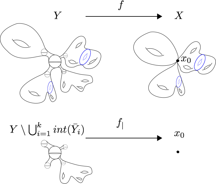
By construction, $X$ can be presented as $X=\sqcup_{i=1}^{k}Y_{i}/\sim$ where $y\sim z$ if and only if $y=y_{i}$ and $z=y_{j}$ for some choice of $1\leq i,j\leq k$. Then $x_{0}=[y_{i}]_{\sim}$ (for any choice of $i=1,...,k$). Let $q:\sqcup_{i=1}^{k}Y_{i}\rightarrow X$ be the quotient map. Let $d_{\delta}$ be the unique length metric such that $q|_{Y_{i}}:(Y_{i},g_{\delta}^{i})\rightarrow(X,d_{\delta})$ is an isometry. Since the metric space $(X,d_{\delta})$ is semi-locally simply connected, it has a universal covering $p:(\widetilde{X},\tilde{d}_{\delta})\rightarrow(X,d_{\delta})$, which has a Riemannian structure except at those points in $p^{-1}(x_{0})=\pi_{1}(X).\tilde{x}_{0}$ where $\tilde{x}_{0}$ is a chosen preimage of $x_{0}$.

5.1.1 The universal cover $\widetilde{X}$

  

Figure 5.2: Intersection of $k=3$ leaves in the universal cover.

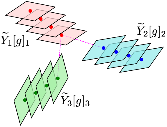
We now introduce some notation in order to efficiently describe the universal cover of the singular space $X$, and the action by automorphisms of its fundamental group. We remark that, by construction, the fundamental group of $X$ splits as a free product: $\pi_{1}(X)\simeq\pi_{1}(Y_{1})\ast\dots\ast\pi_{1}(Y_{k})$. Let us denote by $G=\pi_{1}(X,x_{0})$ and by $G_{j}=(\iota_{j})_{*}\pi_{1}(Y_{j},y_{j})$ where $\iota_{j}:Y_{i}\hookrightarrow X$ is the natural inclusion. Let $\tilde{x}_{0}\in\widetilde{X}$ be a lift of $x_{0}\in X$. Roughly speaking, $\widetilde{X}$ consists of $G/G_{i}$ copies of the universal cover $\widetilde{Y}_{i}$ of each manifold $Y_{i}$, glued along the points of the orbit $G.\tilde{x}_{0}$. Let us summarize the structure of $\widetilde{X}$ in the next proposition:

Proposition 5.2 (On the structure of $\widetilde{X}$).

The universal covering $\widetilde{X}$ of $X$ is obtained as follows:

$$\widetilde{X}=\bigsqcup_{\mathclap{\begin{subarray}{c}i=1,...,k\\ [g]_{i}\in G/G_{i}\end{subarray}}}\widetilde{Y}_{i}[g]_{i}$$

where each $\tilde{Y}_{i}[g]_{i}$ is homeomorphic to $\tilde{Y}_{i}$.
Moreover, $\widetilde{Y}_{i}[g]_{i}\cap\widetilde{Y}_{i}[g^{\prime}]_{i}=\varnothing$ if $[g]_{i}\neq[g^{\prime}]_{i}$ and $\widetilde{Y}_{i}[g]_{i}\cap\widetilde{Y}_{j}[g^{\prime}]_{j}\neq\varnothing$ if and only if either $g^{-1}g^{\prime}\in G_{i}$ or $(g^{\prime})^{-1}g\in G_{j}$ and their intersection is either $\{gh_{i}.\tilde{x}_{0}\}$ for some $h_{i}\in G_{i}$ or $\{g^{\prime}h_{j}.\tilde{x}_{0}\}$ for some $h_{j}\in G_{j}$. Finally, notice that for every $g\in G$ the point $g.\tilde{x}_{0}$ belongs to $\widetilde{Y}_{1}[g]_{1},\dots\widetilde{Y}_{k}[g]_{k}$.

Remark 5.3.

Let us observe that using the notation introduced above:

• $h.\widetilde{Y}_{i}[g]_{i}=\widetilde{Y}_{i}[h\,g]_{i}$;

• for every $i=1,..,k$ we have $p^{-1}(\tilde{x}_{0})\cap\widetilde{Y}_{i}[g]_{i}=\{g\,h_{i}.\tilde{x}_{0}\,|\,h_{i}\in G_{i}\}$;

5.1.2 The distance function $\tilde{d}_{\delta}(\cdot,\cdot)$

First of all remark that, by construction, the distance function $\tilde{d}_{\delta}$ on the singular space $\widetilde{X}$ restricts at any leaf $\widetilde{Y_{i}}[g]$ to the distance $\tilde{g}_{\delta}^{i}$ corresponding to the Riemannian metric on $(\widetilde{Y}_{i},\tilde{g}_{\delta}^{i})$. Moreover,

Lemma 5.4.

$(\widetilde{X},d^{\widetilde{X}}_{\varepsilon})$ is a $\mbox{CAT}(0)$ space.

The Lemma is a classical result about $CAT(\kappa)$ spaces: indeed, the gluing of two locally $CAT(\kappa)$ spaces along convex subsets is still a locally $CAT(\kappa)$ space (see [BH99], Chapter II.11, Theorem 11.1).

Figure 5.3: The three possible configurations for the vertices of a triangle in $X$.

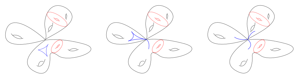
5.1.3 Geodesic balls in $(\widetilde{X},\tilde{d}_{\delta})$

Let $\tilde{x}\in\widetilde{X}$ be any point in the universal cover of $X$, and fix $R\in\mathbb{R}^{+}$. It is worth for the sequel to have a good intuition of what the geodesic ball $B_{\widetilde{X}}(\tilde{x},R)$ looks like. Roughly speaking, the ball of radius $R$ centred at any point $\tilde{x}$ is the union of some metric balls with respect to the metrics $\widetilde{g}_{\delta}^{i}$ defined on each leaf $\widetilde{Y_{i}}[g]_{i}$. More precisely, pick a point $\tilde{x}\in\widetilde{Y}_{i}[g]_{i}$ and fix $R\in\mathbb{R}^{+}$. By construction, $\widetilde{Y}_{i}[g]_{i}$ is a copy of $\widetilde{Y}_{i}$, and the restriction of the singular metric $\tilde{d}_{\delta}$ coincides with $\tilde{g}^{i}_{\delta}$.
If $p^{-1}(x_{0})\cap B_{\widetilde{X}}(\tilde{x},R)=\varnothing$, then $B_{\widetilde{X}}(\tilde{x},R)\subset\widetilde{Y}_{i}[g]_{i}$. Otherwise, the Riemannian ball $B_{\widetilde{Y}_{i}[g]_{i}}(\tilde{x},R)=B_{\widetilde{X}}(\tilde{x},R)\cap\widetilde{Y}_{i}[g]_{i}$ ramifies at points $g\,h_{i,\ell}.\tilde{x}_{0}$ where $h_{i,\ell}$ is an element of $G_{i}$ for every $\ell=1,...,\ell_{i,1}$, and for every $j=1,...,k$ the intersection $B_{\widetilde{X}}(\tilde{x},R)\cap\widetilde{Y}_{j}[g\,h_{i,\ell}]_{j}$ coincides with the Riemannian ball $B_{\widetilde{Y}_{j}[g\,h_{i,\ell}]_{j}}(gh_{i,\ell}.x_{0},R-\tilde{d}_{\delta}(x,gh_{i,\ell}.x_{0}))$. The balls keep ramifying until there are no singular points in its restriction to the leaves. In the end we obtain the following description (see Figure 5.4 for an evoking image):

$$B_{\widetilde{X}}(\tilde{x},R)=B_{\widetilde{Y}_{i}[g_{i}]}(\tilde{x},R)\bigcup_{\begin{subarray}{c}g^{\prime}\in G\,:\\ \tilde{d}_{\delta}(\tilde{x},g^{\prime}\tilde{x}_{0})<R\end{subarray}}\bigcup_{j=1}^{k}B_{\widetilde{Y}_{j}[g^{\prime}]_{j}}(g^{\prime}\tilde{x}_{0},R-\tilde{d}_{\delta}(\tilde{x},g^{\prime}\tilde{x}_{0}))$$

Figure 5.4: Metric ball in the universal cover $\widetilde{X}$ of the singular space $X$ associated with a $3$-manifold having two components of hyperbolic type.

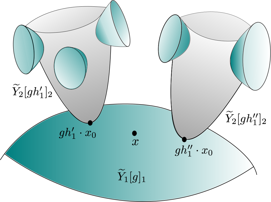
5.2 Barycenter in a CAT(0) space

In this section we shall adapt the notion of barycenter of a measure in the wider context of $CAT(0)$ spaces. The resulting notion will generalize the one in [BCG95] and [Sam99]. To start with, we shall derive an elementary result of Euclidean geometry, which turns out to be fundamental in defining the generalized version of the barycenter. First of all, we introduce some notation. We shall denote with capitol letters points in the Euclidean space $\mathbb{E}^{n}$ and with tiny letters points in other metric spaces. Moreover, given three points $A,B,C$ we will denote by $[A,B,C]$ the triangle in $\mathbb{E}^{n}$ having them as vertices, while given $a,b,c$ we will denote by $[a,b,c]$ the geodesic triangle having them as vertices. Moreover, in the Euclidean space we will denote by $AB$ the segment with endpoints $A$ and $B$, and with $\overset{\rightarrow}{AB}$ the oriented segment with endpoints $A$ and $B$, parameterized so that $A$ is its source and $B$ is its target. Moreover, we will denote by $[a,b]$ the geodesic segment joining $a$ and $b$. Finally, we denote by $AB^{2}$ the square length of the segment $AB$.

Lemma 5.5.

Let $[A,B,C]$ be a triangle in the $\mathbb{E}^{n}$, and take a point $M$ on the side $[B,C]$. Then, the following relation between the lengths of the sides holds:

$$AM^{2}+BM\cdot CM=AB^{2}\cdot\frac{CM}{BC}+AC^{2}\cdot\frac{BM}{BC}$$

Proof.

Let us parameterize the side $BC$ as the interval $[0,1]$, and choose $t\in[0,1]$ such that $\overset{\rightarrow}{BM}=t\cdot\overset{\rightarrow}{BC}$ and $\overset{\rightarrow}{MC}=(1-t)\cdot\overset{\rightarrow}{BC}$ . Let us denote by $\overset{\rightarrow}{AM}^{2}=\langle\overset{\rightarrow}{AC},\overset{\rightarrow}{AC}\rangle$. Then we have:

$$\!\!\!\!\!\!\!\!\!\!\overset{\rightarrow}{AM}^{2}=(\overset{\rightarrow}{AB}+\overset{\rightarrow}{BM})^{2}=(\overset{\rightarrow}{AB}+t\overset{\rightarrow}{BC})^{2}=\overset{\rightarrow}{AB}^{2}+t^{2}\overset{\rightarrow}{BC}+2t\langle\overset{\rightarrow}{AB},\overset{\rightarrow}{BC}\rangle$$ (5.1)

Similarly,

$$\!\!\!\!\!\!\!\!\!\!\overset{\rightarrow}{AM}^{2}=(\overset{\rightarrow}{AC}+\overset{\rightarrow}{CM})^{2}=(\overset{\rightarrow}{AC}+(1-t)\overset{\rightarrow}{BC})^{2}=\overset{\rightarrow}{AB}^{2}+(1-t)^{2}\overset{\rightarrow}{BC}-2(1-t)\langle\overset{\rightarrow}{AC},\overset{\rightarrow}{BC}\rangle$$ (5.2)

Putting together Equations 5.1 and 5.2, we finally get:

$$\overset{\rightarrow}{AM}^{2}=(1-t)\overset{\rightarrow}{AM}^{2}+t\overset{\rightarrow}{AM}^{2}=$$

$$=(1-t)\overset{\rightarrow}{AB}^{2}+t^{2}(1-t)\overset{\rightarrow}{BC}^{2}+t\overset{\rightarrow}{AC}^{2}+t(1-t)^{2}\overset{\rightarrow}{BC}^{2}+2t(1-y)\langle\overset{\rightarrow}{AB}-\overset{\rightarrow}{AC},\overset{\rightarrow}{BC}\rangle=$$

$$=(1-t)\overset{\rightarrow}{AB}^{2}+t^{2}(1-t)\overset{\rightarrow}{BC}^{2}+t\overset{\rightarrow}{AC}^{2}+t(1-t)^{2}\overset{\rightarrow}{BC}^{2}+2t(1-y)\langle\overset{\rightarrow}{AB}-\overset{\rightarrow}{AC},\overset{\rightarrow}{BC}\rangle=$$

$$=(1-t)\overset{\rightarrow}{AB}^{2}+t^{2}(1-t)\overset{\rightarrow}{BC}^{2}+t\overset{\rightarrow}{AC}^{2}+t(1-t)^{2}\overset{\rightarrow}{BC}^{2}+2t(1-y)\langle\overset{\rightarrow}{BC},\overset{\rightarrow}{BC}\rangle=$$

Hence,

$$\overset{\rightarrow}{AM}^{2}=(1-t)\overset{\rightarrow}{AB}^{2}+t\overset{\rightarrow}{AC}^{2}-t(1-t)\overset{\rightarrow}{BC}^{2},$$

and the required equality holds plugging $t=\frac{BM}{BC}$ and $(1-t)=\frac{CM}{BC}$ in the last one. ∎

Lemma 5.6.

Let $(X,d)$ be a $CAT(0)$ space, let $[a,b,c]$ be any geodesic triangle. Then, for any $m\in[b,c]$ the following inequality holds:

$$d(a,m)^{2}+d(m,b)\cdot d(c,m)\leq d(a,b)^{2}+\frac{d(c,m)}{d(b,c)}+d(a,c)^{2}\cdot\frac{d(b,m)}{d(b,c)}.$$

Proof.

Let us construct the comparison triangle $[A,B,C]$ for $[a,b,c]$ in the Euclidean space. Let $M$ be the point dividing the segment $[B,C]$ in the same proportion as $m$ divides $[b,c]$. By the definition of comparison triangle we have: $AB=d(a,b),$ $AC=d(a,c),BC=d(b,c)$ and by construction $BM=d(b,m)$ and $CM=d(c,m)$. Furthermore, the $CAT(0)$ assumption implies $AM\geq d(a,m)$, and we get:

$$d(a,m)^{2} \leq AM^{2}=AB^{2}\cdot\frac{CM}{BC}+AC^{2}\cdot\frac{BM}{BC}-BM\cdot CM$$

$$= d(a,b)^{2}\cdot\frac{d(c,m)}{d(b,c)}+d(a,c)^{2}\cdot\frac{d(b,m)}{d(b,c)}-d(b,m)\cdot d(c,m)$$

∎

Now we shall exploit the previous lemma to prove the existence and uniqueness of the barycenter.

Proposition 5.7.

Let $\mu$ be a positive measure on a $CAT(0)$ space $(X,d)$ such that there exists a point $x_{0}$ satisfying:

$$\int_{X}(1+d(x_{0},z))^{2}d\mu(z)<+\infty$$ (5.3)

and consider the associated Leibniz function

$$B_{\mu}(x)=\int_{X}d^{2}(x,z)d\mu(z).$$

This function is continuous on $X$ and $B_{\mu}(x)\rightarrow+\infty$ when $d(x,x_{0})\rightarrow+\infty$. Moreover, the following conditions hold:

• the function $B_{\mu}$ has a unique minimum point $\operatorname{bar}[\mu]$, called the barycenter of $\mu$;

• for any $x\in X$, we have

  $$d^{2}(\operatorname{bar}[\mu],x)\cdot\mu(X)\leq B_{\mu}(x)-B_{\mu}(\operatorname{bar}[\mu]).$$

Remark 5.8.

We remark that the hypothesis provided by Inequality 5.3 simultaneously ensures that $\mu$ is a finite measure on $X$, and the functions $\rho_{x_{0}}(\cdot)=d(x_{0},\cdot)$ and $\rho_{x_{0}}^{2}$ are in $L^{1}(X,\mu)$.

Proof of Propositon 5.7.

Let us show first that the function $B_{\mu}$ is continuous on X. Let us fix $x_{0}\in X$. For $x\in B(x_{0},R)$ the following chain of estimates holds:

$$d^{2}(x,z)\leq(d(x,x_{0})+d(x_{0},z))^{2}\leq(R+d(x_{0},z))^{2}\leq R^{2}(1+d(x_{0},z))^{2}=f_{R}(z)$$

The function $f_{R}$ does not depend on $x\in B(x_{0},R)$, and is $\mu$-integrable by assumption. Hence for $\{x_{k}\}_{k\in\mathbb{N}}\subset B(x_{0},R)$ such that $x_{k}\rightarrow x$ the $\mu$-integrable functions $d^{2}(x_{k},\cdot)$ are converging pointwise to the $\mu$-integrable function $d^{2}(x_{0},\cdot)$ and are smaller than or equal to $f_{R}$. Thus Lebesgue’s Dominated Convergence Theorem implies the continuity of $B_{\mu}$.

Now, remark that $B_{\mu}(x)\longrightarrow+\infty$ as $d(x_{0},x)\longrightarrow\infty$. Indeed, recalling the elementary inequality $(a-b)^{2}\geq\frac{1}{2}a^{2}-b^{2}$ , we get

$$B_{\mu}(x) \geq \int_{X}(d(x,x_{0})-d(x_{0},z))^{2}d\mu(z)\geq\frac{1}{2}d(x,x_{0})^{2}\mu(X)-\int_{X}d(x_{0},z)^{2}d\mu(z)$$

$$= \frac{1}{2}d(x,x_{0})^{2}\mu(X)-B_{\mu}(x_{0}).$$

We conclude observing that $B_{\mu}(x_{0})<\infty$, and by assumption $d(x,x_{0})\rightarrow\infty$.

Existence. The last two properties imply that there exist points $b\in X$ such that $B_{\mu}(b)=\underset{x\in X}{\inf}B_{\mu}(x)$; namely there exists at least a minimum for the function $B_{\mu}$. Now we shall prove that this minimum value is attained at a unique point.

Uniqueness. Let $b\in X$ be a point as above, i.e., a point realizing the minimum for the function $B_{\mu}$. Then Lemma 5.6 implies that, for any $x,z\in X$ and for any $m\in[b,x]$ (where by $[b,x]$ we intend the —unique— geodesic segment joining the two points) we have:

$$d(m,z)^{2}\leq d(b,z)^{2}\cdot\frac{d(m,x)}{d(b,x)}+d(x,z)^{2}\cdot\frac{d(b,m)}{d(b,x)}-d(m,b)d(m,x).$$

Integrating the last inequality with respect to the measure $\mu$, we get:

$$B_{\mu}(b)\leq B_{\mu}(m)\leq B_{\mu}(b)\cdot\frac{d(m,x)}{d(b,x)}+B_{\mu}(x)\cdot\frac{d(b,m)}{d(b,x)}-d(b,m)d(m,x)\mu(X),$$

where the first inequality holds as $b$ is a minimum for $B_{\mu}$. Thus we have:

$$B_{\mu}(b)\cdot\frac{d(b,m)}{d(b,x)}\leq B_{\mu}(x)\cdot\frac{d(b,m)}{d(b,x)}-d(b,m)d(m,x)\mu(X).$$

Multiplying the last relation by $\frac{d(b,x)}{d(m,b)}$ and letting the distance $d(b,m)$ go to zero, we obtain:

$$B_{\mu}(b)\leq B_{\mu}(x)-d^{2}(b,x)\mu(X),$$

which is clearly equivalent to

$$d^{2}(b,x)\mu(X)\leq B_{\mu}(x)-B_{\mu}(b).$$ (5.4)

We stress here that Inequality (5.4) is precisely the point $(ii)$ of the statement. Now assume that $b$ and $b^{\prime}$ are two points where the function $B_{\mu}$ achieves its minimum. Then Inequality (5.4) implies:

$$d(b,b^{\prime})^{2}\mu(X)\leq B_{\mu}(b^{\prime})-B_{\mu}(b)=0,$$

whence $d(b,b^{\prime})=0$ and $b=b^{\prime}$. This completes the proof of the uniqueness statement. ∎

5.3 The natural maps

Let $g$ be any Riemannian metric on $Y$; we shall denote by $d$ the Riemannian distance on $Y$ and by $\tilde{g},\tilde{d}$ the Riemannian metric and distance on $\widetilde{Y}$ respectively. Moreover, for every $i=1,\dots k$ we shall denote $g^{i}_{\delta}$ the sequence of Riemannian metrics on the irreducible manifold $Y_{i}$ constructed as in Chapter LABEL:section_a_conjectural_minimizing_sequence_irreducible. Furthermore, we denote by $\rho_{\delta,z}(.)=\tilde{d}_{\delta}(z,\,\cdot)$, the distance function from a fixed point $z\in\widetilde{X}$. Let us consider the following immersion of $\widetilde{Y}$ into the space $\mathcal{M}(Y,g)$ of finite, positive Borel measures on $\widetilde{Y}$:

$$y\mapsto d\mu_{c,y}(y^{\prime}):=e^{-c\,\tilde{d}(y,y^{\prime})}dv_{\tilde{g}}(y^{\prime}),$$

for $c>\operatorname{Ent}(g)$ and let

$$\tilde{f}:(\widetilde{Y},\tilde{g})\longrightarrow(\widetilde{X},\tilde{d}_{\delta})$$

be the lift of the quotient map $f$. Then we compose the latter map with the push-forward via $\tilde{f}$, thus obtaining the (finite, positive, Borel) measures $\tilde{f}_{*}\mu_{c,y}$ in $\mathcal{M}(\widetilde{X},\tilde{d})$. Let $B_{c,y}^{\delta}$ denote the Leibniz function associated with the measure $\tilde{f}_{*}\mu_{c,y}$, that is:

$$B_{c,y}^{\delta}(x)=\int_{\widetilde{X}}[\rho_{\delta,x}(z)]^{2}\,d(\tilde{f}_{\ast}\mu_{c,y})(z)=\int_{\widetilde{Y}}(\rho_{\delta,x}(\tilde{f}(y^{\prime})))^{2}e^{-c\tilde{d}(y,y^{\prime})}dv_{\tilde{g}}(y^{\prime}).$$

Since $(\widetilde{X},\tilde{d}_{\delta})$ is a $CAT(0)$ space (Lemma 5.4) it follows from Proposition 5.7 that $B_{c,y}^{\delta}$ admits a unique minimum point for every $y\in\widetilde{Y}$. Hence, for every $y\in\widetilde{Y}$ we define the map

$$\widetilde{F}_{c,\delta}:(\widetilde{Y},\tilde{g})\rightarrow(\widetilde{X},\tilde{d}_{\delta}),\qquad\widetilde{F}_{c,\delta}(y)=\operatorname{bar}[\tilde{f}_{*}\mu_{c,y}]$$

and we shall refer to the maps $\widetilde{F}_{c,\delta}$ as to the natural maps on $(\widetilde{X},d_{\delta})$.

5.4 Properties of the natural maps

We shall now list the properties of the natural maps $\widetilde{F}_{c,\delta}$.

5.4.1 Equivariance, homotopy type, surjectivity

To begin with, we shall observe that the natural maps $\widetilde{F}_{c,\delta}$ are $\lambda$-equivariant, where $\lambda=f_{*}:\pi_{1}(Y,y_{0})\rightarrow\pi_{1}(X,x_{0})$ is the homomorphism induced by $f$ —where $y_{0}\in f^{-1}(x_{0})$.

Lemma 5.9 (Equivariance).

Choose a point $y_{0}\in f^{-1}(x_{0})\subset Y$. The natural maps $\widetilde{F}_{c,\delta}$ are $\lambda$-equivariant with respect to the surjective homomorphism $\lambda=f_{*}:\pi_{1}(Y,y_{0})\rightarrow\pi_{1}(X,x_{0})$

Proof.

As in the irreducible case we have that $B_{c,h.y}^{\delta}(\lambda(h).x)=B_{c,y}^{\delta}(x)$, and thus we obtain the $\lambda$-equivariance of the natural maps. ∎

Since the maps $\widetilde{F}_{c,\delta}$ are $\lambda$-equivariant, they induce maps $F_{c,\delta}:Y\rightarrow X$ between the quotients. Now observe that:

Lemma 5.10 (Homotopy type).

For every $\delta>0$ and every $c>0$ the natural map $F_{c,\delta}$ is homotopic to $f$.

Proof.

The proof goes as in the irreducible case, once observed that $X$ is an aspherical $CW$-complex. ∎

Finally, we observe that:

Lemma 5.11 (Surjectivity).

For every $\delta>0,c>\operatorname{Ent}(g)$ the natural map $F_{c,\delta}$ is surjective.

Proof.

Observe that $H_{3}(X,\mathbb{Z})\cong\mathbb{Z}^{k}=(\iota_{1})_{*}[Y_{1}]\mathbb{Z}\oplus\cdots\oplus(\iota_{k})_{*}[Y_{k}]\,\mathbb{Z}$ where $\iota_{i}:Y_{i}\hookrightarrow X$ is the natural inclusion. For every $i=1,..,k$ let us denote by $p_{i}:X\rightarrow Y_{i}$ the map sending $Y_{i}$ identically into $Y_{i}$ and $X\smallsetminus Y_{i}$ into $y_{i}$ (the point on $Y_{i}$ identified to $x_{0}$). Let us consider $\alpha_{X}=(\iota_{1})_{*}[Y_{1}]\oplus\cdots\oplus(\iota_{k})_{*}[Y_{k}]\in H_{3}(X,\mathbb{Z})$, then $(p_{i})_{*}(\alpha_{X})=[p_{i}(X)]=[Y_{i}]\in H_{3}(Y_{i},\mathbb{Z})$. Moreover, we have that $f_{*}[Y]=\alpha_{X}$. On the other hand, for every $i=1,...,k$ the map $p_{i}\circ F_{c,\delta}$ is homotopic to the map $p_{i}\circ f$, hence $(p_{i}\circ F_{c,\delta})_{*}[Y]=[Y_{i}]$ —i.e. $p_{i}\circ F_{c,\delta}$ has degree $1$, which implies the surjectivity of the map $p_{i}\circ F_{c,\delta}$. Since this holds for every $i=1,...,k$ and the space $X$ is obtained by identifying for $i=1,\dots,k$ the points $\{y_{i}\}$ to $x_{0}$ we conclude that $F_{c,\delta}$ is surjective. ∎

5.4.2 Regularity

In this paragraph we shall be concerned with derivatives of the $\widetilde{F}_{c,\delta}$’s wherever this makes sense. Notice that $\widetilde{X}$ has a Riemannian manifold structure outside the set $S_{x_{0}}=p^{-1}(x_{0})$. Hence, it makes sense to consider derivatives outside this set. Notice that, since we are dealing with a singular space, we have to face some difficulties concerning the regularity of the distance function. In this section we shall explain how this issue can be circumvented. We start proving the following lemma.

Lemma 5.12 (Regularity).

The function $B_{c,y}^{\delta}(x)$ is $C^{2}$ on $\widetilde{X}\setminus S_{x_{0}}$.

Since $B_{c,y}^{\delta}$ is obtained by integrating $(\tilde{\rho}_{\delta,x})^{2}$, Lemma 5.12 is a consequence of the next Lemma, concerning the regularity of the function $\tilde{\rho}_{\delta,z}=\tilde{d}_{\delta}(z,\cdot)$, and of Lebesgue’s Dominated Convergence Theorem.

Lemma 5.13.

Let $z\in\widetilde{X}$ be any point. The function $\tilde{\rho}_{\delta,z}:\widetilde{X}\longrightarrow\mathbb{R}^{+}$ is $C^{2}$ on $\widetilde{X}\smallsetminus S_{x_{0}}.$

Proof.

Let $x\in\widetilde{X}\smallsetminus S_{x_{0}}$. Assume that $z\in\widetilde{Y}_{i}[g]_{i}$ and $x\in\widetilde{Y}_{j}[g^{\prime}]_{j}$. Since $\widetilde{Y}_{i}[g]_{i}$, $\widetilde{Y}_{j}[g^{\prime}]_{j}$ are convex subsets of $(\widetilde{X},\tilde{d}_{\delta})$ we can define $P_{i,g}$, $P_{j,g^{\prime}}$ as the projections on these subsets. By construction it is readily seen that $P_{i,g}(x)=(g\cdot h_{i}).\tilde{x}_{0}$ and $P_{j,g^{\prime}}(z)=(g^{\prime}\cdot h_{j}).\tilde{x}_{0}$, for suitably chosen $h_{i}$, $h_{j}$ (depending only on $\widetilde{Y}_{i}[g]_{i}$, $\widetilde{Y}_{j}[g^{\prime}]_{j}$). Then,

$$\tilde{\rho}_{\delta,z}(x)=\tilde{d}_{\delta}(x,z)=\tilde{d}_{\delta}(z,P_{i,g}(x))+\tilde{d}_{\delta}(P_{i,g}(x),P_{j,g^{\prime}}(z))+\tilde{d}_{\delta}(P_{j,g^{\prime}}(z),x).$$

Notice that, once $z$ has been fixed, the first summand $\tilde{d}_{\delta}(z,P_{i,g}(x))$ and the second summand $\tilde{d}_{\delta}(P_{i,g}(x),P_{j,g^{\prime}}(z))$ are constant as long as $x$ varies in $\widetilde{Y}_{j}[g^{\prime}]_{j}$. Moreover, by construction, the restriction of $\tilde{d}_{\delta}$ to $\widetilde{Y}_{i}[g]_{i}$ is equal to the Riemannian distance function on $(\widetilde{Y}_{i},\tilde{g}_{\delta}^{i})$ (and similarly the restriction of $\tilde{d}_{\delta}$ to $\widetilde{Y}_{j}[g^{\prime}]_{j}$). Hence, there exists a constant $K=K(z,g,g^{\prime})$ such that

$$\tilde{\rho}_{\delta,z}(x)=K+\tilde{d}_{\delta}(x,P_{j,g^{\prime}}(z))$$ (5.5)

for every point $x\in\widetilde{Y}_{j}[g^{\prime}]_{j}$. By this remark, it is clear that we can take derivatives up to the second order (recall that the Riemannian metrics $\tilde{g}_{\delta}^{i}$’s are $C^{2}$) of $\tilde{\rho}_{\delta,z}$ at every point $x\in\widetilde{X}\smallsetminus S_{x_{0}}$, using the Levi-Civita connection with respect to the metric $\tilde{g}_{\delta}^{j}$ of the appropriate leaf $\widetilde{Y}_{j}[g^{\prime}]_{j}$ to which $x$ belongs. ∎

Since we arleady know that for every $y\in\widetilde{Y}$ the minimum of $B_{c,y}^{\delta}$ is attained at unique point, i.e. the barycentre $\widetilde{F}_{c,\delta}(y)$ of the measure $\tilde{f}_{*}\mu_{c,y}$, Lemma 5.12 allows us to give the following characterization of $\widetilde{F}_{c,\delta}(y)$ when $\widetilde{F}_{c,\delta}(y)\in\widetilde{X}\smallsetminus S_{x_{0}}$. The proofs of the following Lemmata 5.14, 5.15 and 5.16 follow exactly the same line as those of Lemmata 4.6, 4.7 and 4.8 in Chapter 4.

Lemma 5.14 (The implicit equation at manifold points).

For every $\delta>0$, $c>\operatorname{Ent}(g)$ and every $y\in\widetilde{Y}$ such that $x=\widetilde{F}_{c,\delta}(y)\in\widetilde{X}\smallsetminus S_{x_{0}}$, the point $x$ is characterized by the equation:

$$\int_{\widetilde{X}}\tilde{\rho}_{\delta,z}(x)d(\tilde{\rho}_{\delta,z})_{x}(v)d(\tilde{f}_{*}\mu_{c,y})(z)=0,\qquad\forall v\in T_{x}\widetilde{X}$$ (5.6)

In other words, the map $\widetilde{F}_{c,\delta}$ is univocally determined on the complement of the preimage of the singular set $S_{x_{0}}$ by the vectorial implicit equation $G_{c,\delta}(\widetilde{F}_{c,\delta}(y),y)=0$, where $G_{c,\delta}=(G_{c,\delta}^{i}):(\widetilde{X}\smallsetminus S_{x_{0}})\times\widetilde{Y}\longrightarrow\mathbb{R}^{n}$ is defined as

$$G_{c,\delta}^{i}(x,y)=\frac{1}{2}\int_{\widetilde{Y}}d_{x}[(\tilde{\rho}_{\delta,\tilde{f}(y^{\prime})}]^{2}(E_{i})e^{-c\tilde{d}(y,y^{\prime})}dv_{\tilde{g}}(y^{\prime}),$$

where $\{E_{i}\}_{i=1}^{n}$ is a global $\tilde{g}_{\delta}^{j}$-orthonormal basis for the tangent space $T_{x}\widetilde{X}$ where $x\in\widetilde{Y}_{j}[g^{\prime}]_{j}$ for some $j$, and $\rho_{\delta,\tilde{f}(y^{\prime})}(\cdot)=\tilde{d}_{\delta}(\tilde{f}(y^{\prime}),\cdot)$.

Since $x\in\widetilde{X}\smallsetminus S_{x_{0}}$ we are allowed to take derivatives (up to the first order) of the function $G_{c}(x,y)$. Hence, for those $y\in\widetilde{Y}$ such that $x=\widetilde{F}_{c,\delta}(y)\in\widetilde{X}\smallsetminus S_{x_{0}}$ we have:

Lemma 5.15 (Derivatives of the implicit function $G_{c,\delta}$).

Using the notation introduced above, the map $G_{c,\delta}:(\widetilde{X}\smallsetminus S_{x_{0}})\times\widetilde{Y}\rightarrow\mathbb{R}^{n}$ is $C^{1}$ and for $x=\widetilde{F}_{c,\delta}(y)\in\widetilde{X}\smallsetminus S_{x_{0}}$, the differential $(dG_{c,\delta})_{(x,y)}|_{T_{x}\widetilde{X}}$ is non-singular. Hence, for $x=\widetilde{F}_{c,\delta}(y)\in\widetilde{X}\smallsetminus S_{x_{0}}$ the map $\widetilde{F}_{c,\delta}:\widetilde{Y}\rightarrow\widetilde{X}$ is $C^{1}$ and satisfies:

$$d_{y}\widetilde{F}_{c,\delta}=-\left(dG_{c,\delta}\right)_{(x,y)}|^{-1}_{T_{x}\widetilde{X}}\circ\left(dG_{c,\delta}\right)_{(x,y)}|_{T_{y}\widetilde{Y}}.$$

Furthermore, if $u\in T_{y}\widetilde{Y}$ and $v\in T_{x}\widetilde{X}$ we have:

$$(dG_{c,\delta}^{i})_{(x,y)}(u)=-c\int_{\widetilde{Y}}\tilde{\rho}_{\delta,\tilde{f}(y^{\prime})}(x)\cdot d_{x}(\tilde{\rho}_{\delta,\tilde{f}(y^{\prime})}(E_{i}))\cdot d_{y}\tilde{\rho}_{y^{\prime}}(u)e^{-c\,\tilde{d}(y,y^{\prime})}dv_{\tilde{g}}(y^{\prime})$$

$$(dG_{c}^{i})_{(x,y)}(v)=\frac{1}{2}\int_{\widetilde{Y}}Dd_{x}[\tilde{\rho}_{\delta,\tilde{f}(y^{\prime})}]^{2}(v,E_{i})e^{-c\,\tilde{d}(y,y^{\prime})}dv_{\tilde{g}}(y^{\prime})$$

Finally, we have the following estimate of the Jacobian of the map $\widetilde{F}_{c,\delta}$ at those points $y\in\widetilde{Y}$ such that $\widetilde{F}_{c,\delta}(y)\in\widetilde{X}\smallsetminus S_{x_{0}}$:

Lemma 5.16 (Computation of the Jacobian of $\widetilde{F}_{c,\delta}$ ).

Let us fix $y\in\widetilde{Y}$ such that $x=\widetilde{F}_{c,\delta}(y)\in\widetilde{X}\smallsetminus S_{x_{0}}$ and define

$$\nu_{c,y}^{\delta}(y^{\prime})=\tilde{d}_{\delta}(\tilde{f}(y),\tilde{f}(y^{\prime}))\cdot\mu_{c,y}(y^{\prime}).$$

Furthermore, let us introduce the positive quadratic forms $k_{c,\delta,y}^{X}$, $h_{c,\delta,y}^{X}$ and $h_{c,\delta,y}^{Y}$ defined on $T_{x}\widetilde{X}$, $T_{x}\widetilde{X}$ and $T_{y}\widetilde{Y}$ respectively.

$k_{c,\delta,y}^{X}(v,v)=\frac{1}{\nu_{c,y}^{\delta}(\widetilde{Y})}\int_{\widetilde{Y}}\frac{1}{2}Dd_{x}[\tilde{\rho}_{\delta,\tilde{f}(y^{\prime})}]^{2}(v,v)d\mu_{c,y}(y^{\prime}),\;\;\qquad\forall v\in T_{x}\widetilde{X}$

$h_{c,\delta,y}^{X}(v,v)=\frac{1}{\nu_{c,y}^{\delta}(\widetilde{Y})}\int_{\widetilde{Y}}d_{x}[\tilde{\rho}_{\delta,\tilde{f}(y^{\prime})}]^{2}(v,v)d\nu_{c,y}^{\delta}(y^{\prime}),\qquad\qquad\forall v\in T_{x}\widetilde{X}$

$h_{c,\delta,y}^{Y}(u,u)=\frac{1}{\nu_{c,y}^{\delta}(\widetilde{Y})}\int_{\widetilde{Y}}d_{y}[(\tilde{\rho})_{y^{\prime}}]^{2}(u,u)d\nu_{c,y}(y^{\prime}),\;\;\;\;\;\qquad\qquad\forall u\in T_{y}\widetilde{Y}$
and let us denote by $K_{c,\delta,y}^{X}$, $H_{c,\delta,y}^{X}$ and $H_{c,\delta,y}^{Y}$ the corresponding endomorphisms of the tangent spaces $T_{x}\widetilde{X}$, $T_{x}{\widetilde{X}}$ and $T_{y}\widetilde{Y}$ respectively, and associated to the scalar products $(\tilde{g}_{\delta}^{j})_{x}$ on $T_{x}\widetilde{X}=T_{x}\widetilde{Y}_{j}[g^{\prime}]_{j}$ (where we are assuming $x\in\widetilde{Y}_{j}[g^{\prime}]_{j}$) and $(\tilde{g})_{y}$ on $T_{y}\widetilde{Y}$. Then,

$$\operatorname{Tr}_{\delta}H^{X}_{c,\delta,y}=1,\qquad\qquad\operatorname{Tr}_{\tilde{g}}(H^{Y}_{c,\delta,y})=1$$ (5.7)

and the eigenvalues of $H^{X}_{c,\delta y}$ and $H^{Y}_{c,\delta,y}$ are pinched between $0$ and $1$. Notice that we denoted for simplicity $\operatorname{Tr}_{\delta}$ the trace with respect to the Riemannian metric on $\widetilde{X}\smallsetminus S_{x_{0}}$ given by the restriction of $d_{\delta}$.
Moreover, for any $u\in T_{y}\widetilde{Y}$ and for any $v\in T_{x}\widetilde{X}$ the following inequality between the quadratic forms holds:

$$k_{c,\delta,y}^{X}(d_{y}\widetilde{F}_{c,\delta}(u),v)\leq c\cdot h^{X}_{c,\delta,y}(v,v)\cdot h^{Y}_{c,\delta,y}(u,u),$$ (5.8)

and

$$|\operatorname{Jac}_{y}(\widetilde{F}_{c,\delta})|\leq\frac{c^{n}}{n^{\frac{n}{2}}}\cdot\frac{(\det H^{X}_{c,\delta,y})^{\frac{1}{2}}}{\det K^{X}_{c,\delta,y}}.$$ (5.9)

In the next paragraph we shall obtain an estimate for the Hessian of $\tilde{d}_{\delta}$ outside the singular set, which together with Lemma 5.16 will give the lower bound of the Minimal Entropy in the reducible case.

5.5 The Hessian of $\tilde{\rho}_{\delta,z}$ on $\widetilde{X}\smallsetminus S_{x_{0}}$

By Lemma 5.16, in order to estimate $\operatorname{Jac}\widetilde{F}_{c,\delta}$ we need to provide a good upper bound for the quadratic form $k_{c,\delta,y}^{X}$. To this purpose we shall need an estimate of the Hessian of $\tilde{\rho}_{\delta,z}$ where $z\in\widetilde{X}\smallsetminus S_{x_{0}}$. This will be done by looking at $Hess_{x}(\tilde{\rho}_{\delta,z})$ as the second fundamental form ${\rm II}_{z,R}(x)$ of the distance sphere $S_{\delta}(z,R)$ with center $z$ and radius $R=\tilde{d}_{\delta}(z,x)$, computed at $x$.

Lemma 5.17 (Hessian of $\tilde{\rho}_{\delta,z}$).

Let us fix a point $x\in\widetilde{X}\smallsetminus S_{x_{0}}$ and a point $z\in\widetilde{X}$. Then $\mathrm{II}_{z,R}(x)=Hess_{x}(\tilde{\rho}_{\delta,z})$.

Proof.

Since $x\in\widetilde{X}\smallsetminus S_{x_{0}}$ we know that there exists a unique $i\in\{1,..,k\}$ and a unique $[g]_{i}\in G/G_{i}$ such that $x\in\widetilde{Y}_{i}[g]_{i}$. By construction of $\tilde{d}_{\delta}$ the intersection of the geodesic sphere $S_{\delta}(z,R)$ passing through $x$ with the leaf $\widetilde{Y}_{i}[g]_{i}$ is equal to $S_{\delta}(P_{i,g}(z),R-r)$ where $r=\tilde{d}_{\delta}(P_{i,g}(z),z)$. But $S_{\delta}(P_{i,g}(z),R-r)$ is isometric to a suitable $\tilde{g}_{\delta}^{i}\,$–geodesic sphere of the same radius in $(\widetilde{Y}_{i},\tilde{g}_{\delta}^{i})$. Thus:

$$\mathrm{II}_{z,R}(x)=\mathrm{II}_{P_{i,g}(z),R-r}(x)=Hess_{x}(\tilde{\rho}_{\delta,P_{i,g}(z)}^{i})=Hess_{x}(\tilde{\rho}_{\delta,z}),$$

where in the second equality we denoted by $\tilde{\rho}_{\delta,P_{i,g}(z)}^{i}$ the Riemannian distance function $\tilde{d}_{\delta}|_{\widetilde{Y}_{i}[g]_{i}}$ from the point $P_{i,g}(z)$; the third equality comes from Equation 5.5. ∎

5.6 An approximated version of Rauch’s Comparison Theorem

From now on, we proceed following the same lines of the proof of the irreducible case, paying some extra care due to the presence of the singular points. Recall that we denoted $y_{i}\in Y_{i}$ for $i=1,\dots,k$ the points identified to the singular point $x_{0}\in X$.

Proposition 5.18.

For every $\varepsilon>0$ define $R_{\varepsilon}=\ln\left(\sqrt{\frac{2}{\varepsilon}}\right)$. Assume that $x\in\widetilde{X}\smallsetminus S_{x_{0}}$ is such that, for any $i=1,\dots,k$ and $g\in\pi_{1}(X,x_{0})$, the intersection $B_{\widetilde{X}}(x,R_{\varepsilon})\cap\widetilde{Y}_{i}[g]_{i}$ is either empty or is a hyperbolic ball; then for every $z\in\widetilde{X}$ and $v\in T_{x}\widetilde{X},$ the following inequality holds:

$$(1-\varepsilon)\tilde{\rho}_{\delta,z}\left(||v||_{\delta}^{2}-(d_{x}\tilde{\rho}_{\delta,z}\otimes d_{x}\tilde{\rho}_{\delta,z})(v,v)\right)\leq\tilde{\rho}_{\delta,z}D_{x}d\tilde{\rho}_{\delta,z}(v,v).$$ (5.10)

Proof.

We may assume that $x\in\widetilde{Y}_{i}[g]_{i}$. Recall that we denoted by $P_{g,i}$ the projection onto the convex subspace $\widetilde{Y}_{i}[g]_{i}$. In order to prove Proposition 5.18 we need to distinguish two cases: the case where $P_{i,g}(z)\in B_{\widetilde{Y}_{i}[g]_{i}}(x,R_{\varepsilon})$ and the case where $\tilde{d}_{\delta}(P_{i,g}(z),x)>R_{\varepsilon}$. In the first case, observe that the second fundamental form $\mathrm{II}_{P_{i,g}(z),r}(x)$ of the ball of radius $r=\tilde{d}_{\delta,i}(x,P_{i,g}(z))$ —where we denote with $\tilde{d}_{\delta,i}$ the Riemannian distance function on $\widetilde{Y}_{i}[g]_{i}$— coincides with the second fundamental form in the hyperbolic case. Hence, for $v\in T_{x}\widetilde{X}$

$$Hess_{x}(\tilde{\rho}_{\delta,z})(v,v)=Hess_{x}(\tilde{\rho}^{i}_{\delta,P_{i,g}(z)})(v,v)\geq\tilde{g}_{\delta}^{i}(v,v)-(d_{x}\tilde{\rho}^{i}_{P_{i,g}(z)}(v))^{2},$$

where we used the notation $\tilde{\rho}_{\delta,w}^{i}$ for the Riemannian distance function from $w$ in $(\widetilde{Y}_{i}[g]_{i},\tilde{g}_{\delta}^{i})$. Otherwise, the distance between $P_{i,g}(z)$ and $x$ is greater than $R_{\varepsilon}$, and we can apply Lemma 4.12 in restriction to $\widetilde{Y}_{i}[g]_{i}$, thus obtaining:

$$Hess_{x}(\tilde{\rho}_{\delta,z})(v,v)\geq(1-\varepsilon)\left(\tilde{g}_{\delta}^{i}(v,v)-(d_{x}\tilde{\rho}_{\delta,z}(v))^{2}\right).$$

∎

5.7 The Jacobian estimate

We are now ready to apply the inequalities found in Lemma 5.16 and Proposition 5.18, to derive an almost optimal inequality for the Jacobian of the maps $\widetilde{F}_{c,\delta}$ valid on an appropriately chosen subset of $Y$.

Proposition 5.19 (Jacobian Estimate, reducible case).

For every $\varepsilon>0$ there exists $R_{\varepsilon}>0$ such that, if the ball centred at the non-singular point $x=\widetilde{F}_{c,\delta}(y)\in\widetilde{Y}_{i}[g]_{i}\subset\widetilde{X}$ of radius $R_{\varepsilon}$ is such that $B_{\widetilde{X}}(x,R_{\varepsilon})\cap\widetilde{Y}_{i}[g_{i}]$ is hyperbolic for every $g\in\pi_{1}(X,x_{0})$, and every $i=1,...,k$, the following estimate for the Jacobian holds:

$$\lvert\operatorname{Jac}\widetilde{F}_{c,\delta}(y)\rvert\leq\frac{1}{\left(1-\varepsilon\right)^{n}}\cdot\left(\frac{c}{n-1}\right)^{n}.$$ (5.11)

Proof.

Let $x=\widetilde{F}_{c,\delta}(y)$ and assume that $B_{\widetilde{X}}(x,R_{\varepsilon})$ satisfies the assumptions. Then by Proposition 5.18 we know that, at the point $x=\widetilde{F}_{c,\delta}(y)$ the following inequality holds:

$$(1-\varepsilon)\tilde{\rho}_{\delta,z}\left(||v||_{\delta}^{2}-(d_{x}\tilde{\rho}_{\delta,z}\otimes d_{x}\tilde{\rho}_{\delta,z})(v,v)\right)\leq\tilde{\rho}_{\delta,z}D_{x}d\tilde{\rho}_{\delta,z}(v,v)$$

for every $z\in\widetilde{X}$. Integrating in $d(\tilde{f}_{*}\mu_{c,y})$ and normalizing by $\nu_{c,y}^{\delta}(\widetilde{Y})$ we get the following inequality between quadratic forms

$$(1-\varepsilon)\cdot(\tilde{g}_{\delta}^{i}-h_{c,\delta,y}^{X})\leq k_{c,\delta,y}^{X}$$

and hence we obtain the inequality between the symmetric endomorphisms:

$$(1-\varepsilon)\cdot\left(\operatorname{Id}-H_{c,\delta,y}^{X}\right)\leq K_{c,\delta,y}^{X}$$

Now, using this inequality, Lemma 5.16 and Lemma 4.9 we obtain:

$$\lvert\operatorname{Jac}\widetilde{F}_{c,\delta}(y)\rvert\leq\frac{c^{n}}{n^{\frac{n}{2}}}\cdot\frac{|\det(H_{c,\delta,y}^{X})|^{\frac{1}{2}}}{\det(K_{c,\delta,y}^{X})}\leq$$

$$\leq\frac{c^{n}}{n^{\frac{n}{2}}(1-\varepsilon)^{n}}\frac{|\det(H_{c,\delta,y}^{X})|^{\frac{1}{2}}}{\det(\operatorname{Id}-H_{c,\delta,y}^{X})}\leq\frac{1}{(1-\varepsilon)^{n}}\cdot\left(\frac{c}{n-1}\right)^{n}$$

which is the desired inequality. ∎

5.8 Proof of Theorem 5.1

The proof of Theorem 5.1 partly relies on the proof of Theorem 4.1. For every $i=1,...,k$ and every $j=1,...,n_{i}$ we shall denote by $\{V_{i,\delta,\varepsilon}^{j}\}_{j=1}^{n_{i}}$ the collection of open subsets of $(Y_{i},g_{\delta}^{i})$ constructed in the proof of Theorem 5.1, when $Y_{i}$ does not admit a complete hyperbolic metric. Otherwise we shall choose $V_{i,\delta,\varepsilon}^{1}=Y_{i}$. By construction of the metrics $g_{\delta}^{i}$ (where $g_{\delta}^{i}$ is the —unique— hyperbolic metric for every $Y_{i}$ which is of hyperbolic type) and by Proposition 5.19 we have that:

$$|\operatorname{Jac}F_{c,\delta}(y)|\leq\frac{1}{(1-\varepsilon)^{3}}\cdot\left(\frac{c}{2}\right)^{3}$$

for every $y\in\left(\bigcup_{i=1}^{k}\bigcup_{j=1}^{n_{i}}F_{c,\delta}^{-1}(V_{i,\delta,\varepsilon}^{j})\right)\smallsetminus\{x_{0}\}$. On the other hand we have that for every fixed $\varepsilon>0$ the volume $\operatorname{Vol}(V_{i,\delta,\varepsilon}^{j})$ converges as $\delta\rightarrow 0$ to $\operatorname{Vol}(int(X_{i}^{j}),hyp_{i}^{j})$. Now observe that:

$$\int_{\left(\bigcup_{i=1}^{k}\bigcup_{j=1}^{n_{i}}F_{c,\delta}^{-1}(V_{i,\delta,\varepsilon}^{j})\right)\smallsetminus F_{c,\delta}^{-1}\{x_{0}\}}|\operatorname{Jac}F_{c,\delta}(y)|dv_{g}(y)=$$

$$=\int_{\left(\bigcup_{i=1}^{k}\bigcup_{j=1}^{n_{i}}V_{i,\delta,\varepsilon}^{j}\right)\smallsetminus\{x_{0}\}}\#(F_{c,\delta}^{-1}(x))d\mu_{\delta}(x)=$$

$$=\sum_{i=1}^{k}\int_{\bigcup_{j=1}^{n_{i}}V_{i,\delta,\varepsilon}^{j}}\#(F_{c,\delta}^{-1}(x))dv_{g_{\delta}^{i}}(x)\geq\sum_{i=1}^{k}\sum_{j=1}^{n_{i}}\operatorname{Vol}\left(V_{i,\delta,\varepsilon}^{j},g_{\delta}^{i}\right)$$

where the first equality comes from the coarea formula and the second from the fact that the $V_{i,\delta,\varepsilon}^{j}$’s are disjoint. Plugging the inequality for the Jacobian into the formula, we see that:

$$\sum_{i=1}^{k}\sum_{j=1}^{n_{i}}\operatorname{Vol}\left(V_{i,\delta,\varepsilon}^{j},g_{\delta}^{i}\right)\leq\frac{1}{(1-\varepsilon)^{3}}\cdot\left(\frac{c}{2}\right)^{3}\cdot\operatorname{Vol}(Y,g)$$

Now for every fixed $\varepsilon>0$ the left-hand side of the latter inequality converges to $\sum_{i=1}^{k}\sum_{j=1}^{n_{i}}\operatorname{Vol}(int(X_{i}^{j}),hyp_{i}^{j})$ as $\delta\rightarrow 0$. Since this holds for every choice of $\varepsilon>0$ it is easily seen that:

$$\operatorname{EntVol}(Y,g)\geq 2\cdot\left(\sum_{i=1}^{n}\sum_{j=1}^{n_{i}}\operatorname{Vol}(int(X_{i}^{j}),hyp_{i}^{j})\right)^{1/3}$$ (5.12)

As Inequality (5.12) holds for every Riemannian metric $g$ on $Y$ we have the following estimate from below for $\operatorname{MinEnt}(Y)$:

$$\operatorname{MinEnt}(Y)\geq 2\cdot\left(\sum_{i=1}^{n}\sum_{j=1}^{n_{i}}\operatorname{Vol}(int(X_{i}^{j}),hyp_{i}^{j})\right)^{\frac{1}{3}}.$$

Appendix A Smooth and Riemannian orbifolds

This appendix is devoted to the introduction of smooth and Riemannian orbifolds. For further details, we recommend [BMP03] and [KL14].

A.0.1 Definition and basic notions

Definition A.1.

A smooth $n$-orbifold is a metrizable topological space $\mathcal{O}$ endowed with a collection $\left\{\left(U_{i},\tilde{U}_{i},\phi_{i},\Gamma_{i}\right)\right\}_{i}$, called an atlas, where for every $i$ $U_{i}$ is an open subset of $\mathcal{O}$, $\tilde{U}_{i}$ is an open subset of $\mathbb{R}^{n-1}\times\left[0,\infty\right)$, $\phi_{i}:\tilde{U}_{i}\rightarrow U_{i}$ is a continuous map (called a chart) and $\Gamma_{i}$ is a finite group of diffeomorphisms of $\tilde{U}_{i}$ satisfying the following conditions:

1. The $U_{i}$’s cover $\mathcal{O}$.

2. Each $\phi_{i}$ factors through a homeomorphism between $\tilde{U}_{i}/\Gamma_{i}$ and $U_{i}$.

3. The charts are compatible in the following sense: for every $x\in\tilde{U}_{i}$ and $y\in\tilde{U}_{j}$ with $\phi_{i}(x)=\phi_{j}(y)$, there is a diffeomorphism $\psi$ between a neighbourhood $V$ of $x$ and a neighbourhood $W$ of $y$ such that $\phi_{j}(\psi(z))=\phi_{i}(z)$ for all $z\in V$.

For convenience, we shall assume that the atlas is maximal.

We remark that an orbifold $\mathcal{O}$ is a manifold if all the groups $\Gamma_{i}$ are trivial. Given an orbifold $\mathcal{O}$, we denote by $\lvert\mathcal{O}\rvert$ its underlying space, i.e. the topological space obtained by neglecting the orbifold structure.

Let $x\in\mathcal{O}$ be any point; then the local group of $\mathcal{O}$ at $x$ is the group $\Gamma_{x}$ defined as follows: pick any chart $(U,\tilde{U}_{i},\phi,\Gamma)$, where $x\in U$. Then $\Gamma_{x}$ is the stabilizer of any point of $\phi^{-1}(x)$ under the action of $\Gamma$. It turns out that the group $\Gamma_{x}$ is well defined up to isomorphism. We say that the point $x$ is regular if $\Gamma_{x}$ is trivial, otherwise $x$ is singular. Notice that the set of singular points is empty if and only if $\mathcal{O}$ is a manifold.

There are several notions that can be defined in the orbifold context, extending in a straightforward manner the analogous notion given for manifolds.

The boundary of $\mathcal{O}$, denoted $\partial\mathcal{O}$, is the set of points $x\in\mathcal{O}$ such that there exists a chart at $x$, $\phi_{i}:\tilde{U}_{i}\rightarrow U_{i}$ such that $\phi_{i}^{-1}(x)\subset\mathbb{R}^{n-1}\times\left\{0\right\}$. The orbifold $\mathcal{O}\setminus\partial\mathcal{O}$ is called the interior of $\mathcal{O}$. We call $\mathcal{O}$ orientable if it has an atlas such that each $\phi_{i}$ and every element of each $\Gamma_{i}$ are orientation preserving.

Observation.

Let $\mathcal{O}$ be an orbifold with boundary, and assume that all the singular points are conical points, i.e. the group $\Gamma_{i}\simeq\mathbb{Z}_{k}$ acts by rotation. Let $x$ be a boundary point. Then, there exists a chart $(\tilde{U}_{i},U_{i}.\phi_{i},\Gamma_{i})$ at $x$ such that $\phi_{i}^{-1}(x)\subset\mathbb{R}^{n-1}\times\{0\}$, and the group $\Gamma_{i}$ is trivial. Thus, there is a neighbourhood of the boundary such that the local groups are trivial.

A.0.2 Maps between orbifolds

A map between two orbifolds $\mathcal{O}$ and $\mathcal{O}^{\prime}$ is a continuous map $f:\lvert\mathcal{O}\rvert\rightarrow\lvert\mathcal{O}^{\prime}\rvert$ such that for every $x\in\mathcal{O}$ there are charts $\phi_{i}:\tilde{U}_{i}\rightarrow U_{i}\ni x$ and $\phi_{j}^{\prime}:\tilde{U}^{\prime}_{j}\rightarrow U_{j}^{\prime}$ such that $f(U_{i})\subset U_{j}^{\prime}$ and the restriction $f|_{U_{i}}$ can be lifted to a smooth map $\tilde{f}:\tilde{U}_{i}\rightarrow\tilde{U}^{\prime}_{j}$ which is equivariant with respect to some homomorphism $\Gamma_{i}\rightarrow\Gamma^{\prime}_{j}$. A map $f:\mathcal{O}\rightarrow\mathcal{O}^{\prime}$ is an immersion (resp. a submersion) if the lifts $\tilde{f}$ are immersions (resp. submersions). An embedding is an immersion whose underlying map is a homeomorphism with the image. A diffeomorphism is a surjective embedding.

A.0.3 Orbifold covering

A covering of an orbifold $\mathcal{O}$ is an orbifold $\tilde{\mathcal{O}}$ with a continuous map $p:\lvert\tilde{\mathcal{O}}\rvert\rightarrow\lvert\mathcal{O}\rvert$, called a covering map, such that every point $x\in\mathcal{O}$ has a neighbourhood $U$ with the following property: for each component $V$ of $p^{-1}(U)$ there is a chart $\phi:\tilde{V}\rightarrow V$ such that $p\circ\phi$ is a chart.

We say that an orbifold is good if it is covered by a manifold, bad otherwise. If an orbifold is finitely covered by a manifold we say that it is very good.

The notions of deck transformation group and universal covering extend to the context of orbifolds, see [Thu97] and [BMP03].
The fundamental group of $\mathcal{O}$, denoted by $\pi_{1}^{orb}(\mathcal{O})$, is the deck transformation group of its universal covering.

There is an interpretation of the fundamental group in terms of loops, keeping track of the passage through the singular locus. Furthermore, a continuous map between two orbifolds gives rise to a map between the corresponding orbifold fundamental groups.

A.0.4 Riemannian orbifolds

A Riemannin metric on an orbifold $\mathcal{O}$ is given by an atlas for $\mathcal{O}$ along with a collection of Riemannian metric on the $\tilde{U}_{i}$’s so that:

1. $\Gamma_{i}$ acts isometrically on $\tilde{U}_{i}$ for every $i$;

2. The diffeomorphism $\psi$ is an isometry.

We say that a map $f:\mathcal{O}\rightarrow\mathcal{O}^{\prime}$ between Riemannian orbifolds is a Riemannian submersion (resp. a Riemannian immersion) if the lift $\tilde{f}$ is a Riemannian submersion (resp. a Riemannian immersion) equivariant with respect to the isometric actions of the local groups.

Remark A.2.

Let $\mathcal{O}$ and $\mathcal{O}^{\prime}$ be two orbifolds that are global quotients of two Riemannian manifolds $M$ and $M^{\prime}$ with respect to groups of isometries $\Gamma$ and $\Gamma^{\prime}$ acting properly. Then, a Riemannian submersion between $\mathcal{O}$ and $\mathcal{O}^{\prime}$ is equivalent to a Riemannian submersion between $M$ and $M^{\prime}$ which is equivariant with respect to the action of $\Gamma$ and $\Gamma^{\prime}$.

Appendix B Proof of Proposition 2.8

Lemma B.1.

Let $\Phi\in\mathcal{C}^{1}\left(-\infty,0\right]\cap\mathcal{C}^{1}\left[0,+\infty\right)\cup\mathcal{C}^{0}(\mathbb{R})$ such that:

1. $\Phi^{\prime}(t)\geq 0$ for every $t\not=0$;

2. $|\Phi(0)|\leq M;$

3. $0\leq\Phi^{\prime}(0)^{-}<\Phi^{\prime}(0)^{+}$

Then there exists $\varepsilon>0$, $\varepsilon$ arbitrarily small, such that there exists a function $\Phi_{\varepsilon}\in\mathcal{C}^{1}(\mathbb{R})$ satisfying the following properties:

1. $\Phi_{\varepsilon}(t)=\Phi(t)$ for $t\in\mathbb{R}\setminus\left(-\varepsilon,\varepsilon\right)$ and $\Phi\leq\Phi_{\varepsilon}\leq\Phi(\varepsilon)$ for $t\in\left(-\varepsilon,\varepsilon\right)$

2. $\Phi^{\prime}(-\varepsilon)\leq\Phi^{\prime}_{\varepsilon}(t)\leq\Phi^{\prime}(\varepsilon)$ for every $t\in\left(-\varepsilon,\varepsilon\right)$

3. $\lvert\int_{-\varepsilon}^{\varepsilon}\Phi_{\varepsilon}(s)ds\rvert\leq 2M\varepsilon$

Proof.

Property $iii$ implies that there exists $\varepsilon_{1}$ such that, for $\varepsilon<\varepsilon_{1}$, inequality $\Phi^{\prime}(-\varepsilon)<\Phi^{\prime}(\varepsilon)$ holds. Let us choose $\varepsilon<\varepsilon_{1}$; then it si possible to construct a function $\Phi_{\varepsilon}$ such that $\Phi_{\varepsilon}(\pm\varepsilon)=\Phi(\pm\varepsilon)$, $\Phi_{\varepsilon}^{\prime}(\pm\varepsilon)=\Phi^{\prime}(\pm\varepsilon)$ and $\Phi^{\prime}(-\varepsilon)\leq\Phi^{\prime}(t)\leq\Phi^{\prime}(\varepsilon)$. Furthermore, we can choose $\Phi_{\varepsilon}$ such that $\Phi(-\varepsilon)\leq\Phi_{\varepsilon}(t)\leq\Phi(\varepsilon)$. Moreover, since $|\Phi(0)|<M$ there exists $\varepsilon_{2}$ such that for $\varepsilon<\varepsilon_{2}$ inequality $|\Phi(t)|\leq M$ holds for $t\in(-\varepsilon,\varepsilon)$. Thus, provided $\varepsilon<\min(\varepsilon_{1},\varepsilon_{2})$:

$$\left\lvert\int_{-\varepsilon}^{\varepsilon}\Phi_{\varepsilon}(s)ds\right\rvert\leq\int_{-\varepsilon}^{\varepsilon}\lvert\Phi_{\varepsilon}(s)\rvert ds\leq 2M\varepsilon$$

∎

Lemma B.2.

Let $\varphi\in\mathcal{C}^{2}\left(-\infty,0\right]\cap\mathcal{C}^{2}\left[0,+\infty\right)\cap\mathcal{C}^{1}(\mathbb{R})$ with $\varphi(0)\geq 0$ such that:

1. $\varphi$ convex;

2. $|\varphi^{\prime}(0)|\leq M$;

3. $0\leq\varphi^{\prime\prime}(0)^{-}<\varphi^{\prime\prime}(0)^{+}$

Then there exists $\varepsilon>0$ arbitrarily small and $\varphi_{\varepsilon}\in\mathcal{C}^{2}(\mathbb{R})$ such that:

1. $\varphi^{\prime}(t)\leq\varphi^{\prime}_{\varepsilon}(t)\leq\varphi^{\prime}(\varepsilon)$ for every $t\in\left(-\varepsilon,\varepsilon\right)$ ;

2. $\varphi^{\prime\prime}(-\varepsilon)\leq\varphi_{\varepsilon}^{\prime\prime}(t)\leq\varphi^{\prime\prime}(\varepsilon)$ for $t\in(-\varepsilon,\varepsilon)$;

3. $\left\{\begin{array}[]{l}\varphi_{\varepsilon}=\varepsilon\quad t\leq-\varepsilon\\ \varphi_{\varepsilon}=\varepsilon+c\quad t\geq\varepsilon,|c|<2M\varepsilon\\ |\varphi_{\varepsilon}-\varphi|<3M\varepsilon\end{array}\right.$

Proof.

Denote by $\Phi=\varphi^{\prime}$. Then, $\Phi$ satisfies the hypotheses of Lemma B.1 and applying it we get a function $\Phi_{\varepsilon}$ such that properties a,b,c of Lemma B.1 hold. Let us define:

$$\varphi_{\varepsilon}(t)=\int_{-\varepsilon}^{t}\Phi_{\varepsilon}(s)ds+\varphi(-\varepsilon)$$

We show that $\varphi_{\varepsilon}$ satisfies property $C$.
For $t\leq-\varepsilon$,

$$\varphi_{\varepsilon}(t)=\int_{-\varepsilon}^{t}\Phi_{\varepsilon}(s)ds+\varphi(-\varepsilon)=-\int_{t}^{-\varepsilon}\Phi_{\varepsilon}(s)ds+\varphi(-\varepsilon)=\cancel{-\varphi(-\varepsilon)}+\varphi(t)+\cancel{\varphi(-\varepsilon)}=\varphi(t)$$

Thus $\varphi_{\varepsilon}=\varphi$ for $t\leq-\varepsilon$.
For $t\geq\varepsilon:$

$$\varphi_{\varepsilon}(t)=\int_{-\varepsilon}^{t}\Phi_{\varepsilon}(s)ds+\varphi(-\varepsilon)=\int_{-\varepsilon}^{\varepsilon}\Phi_{\varepsilon}(s)ds+\int_{\varepsilon}^{t}\Phi(s)ds+\varphi(-\varepsilon)=\\ =\int_{-\varepsilon}^{\varepsilon}\Phi_{\varepsilon}(s)ds+\int_{\varepsilon}^{t}\varphi^{\prime}(s)ds+\varphi(-\varepsilon)=\int_{-\varepsilon}^{\varepsilon}\Phi_{\varepsilon}(s)ds+\phi(t)-\phi(\varepsilon)+\varphi(-\varepsilon)=\\ =\phi(t)+c_{1}+c_{2}$$

where $c_{1}=\int_{-\varepsilon}^{\varepsilon}\Phi_{\varepsilon}(s)ds$, $c_{2}=\varphi(-\varepsilon)-\varphi(\varepsilon)$.

Furthermore,

$$\lvert c_{1}+c_{2}\rvert\leq\left\lvert c_{1}\right\rvert+\left\lvert c_{2}\right\rvert\leq\left\lvert\int_{-\varepsilon}^{\varepsilon}\Phi_{\varepsilon}(s)ds\right\rvert+\left\lvert\varphi(-\varepsilon)-\varphi(\varepsilon)\right\rvert\leq 4M\varepsilon$$

where Inequality $\int_{-\varepsilon}^{\varepsilon}\Phi_{\varepsilon}(s)ds\leq 2M\varepsilon$ follows by Lemma B.1.

For $t\in\left(-\varepsilon,\varepsilon\right)$, the same computation just held gives:

$$\lvert\varphi_{\varepsilon}(t)-\varphi(t)\rvert\leq\left\lvert\int_{-\varepsilon}^{t}\Phi_{\varepsilon}(s)ds\right\rvert+\left\lvert\varphi(-\varepsilon)-\varphi(t)\right\rvert\leq 4M\varepsilon$$

Finally, we observe that property a of Lemma B.1 implies the thesis A, and part B of the thesis follows from property b.

∎

Proposition B.3.

For every fixed $\ell,\delta>0$ there exists $\varepsilon>0$ arbitrarily small and $\varphi_{\varepsilon}\in\mathcal{C}^{2}(\mathbb{R})$ such that:

1. $\varphi_{\varepsilon}$ is not increasing and convex, such that

   $\left\{\begin{array}[]{l}\varphi_{\varepsilon}(t)=\varphi_{0}(t)=\ell e^{-t}\,\,\mbox{ for }t\leq-\varepsilon\\ \varphi_{\varepsilon}(t)=\ell^{\prime}\,\,\mbox{ for }t\geq t_{\delta}+\varepsilon\end{array}\right.$
   where:

   $$\ell\frac{\sqrt{\delta(1+\delta)}}{1+2\delta}\leq\ell^{\prime}\leq 4\ell\frac{\sqrt{\delta(1+\delta)}}{1+2\delta}$$

2. $\frac{(\varphi_{\varepsilon}^{\prime})^{2}}{\varphi_{\varepsilon}^{2}}<(1+2\delta)^{2}\frac{(\varphi_{0}^{\prime})^{2}}{\varphi_{0}^{2}}$ for every $t\in\mathbb{R}$

3. $\frac{\varphi_{\varepsilon}^{\prime\prime}}{\varphi_{\varepsilon}}\leq(1+2\delta)^{2}$ for every $t\in(-\varepsilon,t_{\delta}+\varepsilon)$

where $t_{\delta}=\frac{1}{2(1+2\delta)}\ln\left(1+\frac{1}{\delta}\right)$

Proof.

The function $\varphi_{0}(t)=\ell e^{-t}$ satisfies the differential equation $\frac{\varphi_{0}^{\prime\prime}}{\varphi}=1$, with initial conditions

$$\left\{\begin{array}[]{l}\varphi_{0}(0)=\ell\\ \varphi_{0}^{\prime}(0)=-\ell\end{array}\right.$$

Let us denote by $\varphi_{\delta}$ the solution of the differential equation $\frac{\varphi_{\delta}^{\prime\prime}}{\varphi_{\delta}}=\left(1+2\delta\right)^{2}$ with the same initial conditions. Namely,

$$\varphi_{\delta}(t)=\ell\left(\frac{1+\delta}{1+2\delta}\right)e^{-(1+2\delta)t}+\ell\frac{\delta}{1+2\delta}e^{(1+2\delta)t}$$

Straightforward computations show that, for $\delta>0$, the function $\varphi_{\delta}$ is more convex than $\varphi_{0}$, and $\varphi_{\delta}$ has a unique stationary point, which turns to be a minimum, at $t_{\delta}=\frac{1}{2(1+2\delta)}\ln\left(1+\frac{1}{\delta}\right)$. We denote by $\ell_{\delta}$ the corresponding minimal value.

We define the following function:

$$\varphi(t)=\left\{\begin{array}[]{ll}\varphi_{0}(t)&\text{for }t<0\\ \varphi_{\delta}(t)&\text{for }t\in\left[0,\right]\\ \ell_{\delta}&\text{for }t>t_{\delta}\end{array}\right.$$

We observe that $\varphi(t)\in\mathcal{C}^{1}(\mathbb{R})\cap\mathcal{C}^{2}\left(\left(-\infty,0\right]\right)\cap\mathcal{C}^{2}(\left[0,t_{\delta}\right])\cap\mathcal{C}^{2}(\left[t_{\delta},+\infty\right))$, but is not $\mathcal{C}^{2}(\mathbb{R})$. Furthermore, $\varphi$ is not increasing, convex and satisfies condition $(1)$. Moreover, we observe that, for every $\delta>0$:

$$\frac{\varphi_{\delta}^{\prime 2}}{\varphi_{\delta}^{2}}\leq\frac{\varphi_{0}^{\prime 2}}{\varphi_{0}^{2}}.$$ (B.1)

Indeed, on the interval $\left[0,t_{\delta}\right]$ the following inequality holds:

$$\frac{\varphi_{\delta}^{\prime\prime}}{\varphi_{\delta}}\geq\frac{\varphi_{0}^{\prime\prime}}{\varphi_{0}}$$

and $\varphi_{\delta}(0)=\varphi_{0}(0)$, $\varphi_{\delta}^{\prime}(0)=\varphi^{\prime}_{\delta}(0)$. Then, by Sturm-Liouville Theorem, $0>\varphi_{\delta}^{\prime}\geq\varphi_{0}^{\prime}$ and $\varphi_{\delta}\geq\varphi_{0}>0$ and

$$\left\lvert\frac{\varphi_{\delta}^{\prime}}{\varphi}\right\rvert\leq\left\lvert\frac{\varphi_{0}^{\prime}}{\varphi}\right\rvert.$$

The latter Inequality implies Equation B.1. In order to obtain a $\mathcal{C}^{2}$ function satisfying the required properties we will apply (twice) Lemma B.2, as follows.

Firstly, we observe that $\varphi$ satisfies the hypotheses of Lemma B.2; hence, there exists a function $\varphi_{\varepsilon}$, enjoying properties $(A),(B),(C)$. In particular, $\varphi_{\varepsilon}$ is convex, not increasing, and

$$\left\{\begin{array}[]{ll}\varphi_{\varepsilon}=\varphi&\mbox{for }t\leq\varepsilon\\ \varphi_{\varepsilon}=\varphi+c(\varepsilon)&\mbox{for }t\geq\varepsilon\\ \lvert\varphi_{\varepsilon}-\varphi\rvert\leq 3M\varepsilon&\mbox{for }t\in\left[-\varepsilon,\varepsilon\right]\end{array}\right.$$

We claim that $\varphi_{\varepsilon}$ satisfies properties $2)$ and $3)$. Indeed, Lemma B.2 implies:

$$\varphi^{\prime}(t)\leq\varphi^{\prime}_{\varepsilon}(t)\leq\varphi^{\prime}(\varepsilon)$$

for $t\in\left(-\varepsilon,\varepsilon\right)$. Thus:

$$\left(\frac{\varphi_{\varepsilon}^{\prime}(t)}{\varphi_{\varepsilon}(t)}\right)^{2}\leq\left(\frac{\varphi^{\prime}(t)}{\varphi_{\varepsilon}(t)}\right)^{2}\leq\left(\frac{\varphi^{\prime}(t)}{\varphi(t)-3M\varepsilon}\right)^{2}$$

Now choose $\varepsilon\leq\min\left\{\frac{1}{2},\frac{\delta\ell}{6M\sqrt{e}}\right\}$ so that, in particular, $\varepsilon\leq\frac{\delta\varphi(\varepsilon)}{6M}$; then we have

$$\left(\frac{\varphi^{\prime}(t)}{\varphi(t)-3M\varepsilon}\right)^{2}\leq\left(\frac{\varphi^{\prime}(t)}{\left(1-\frac{\delta}{2}\right)\varphi(t)}\right)^{2}$$

Thus,

$$\left(\frac{\varphi_{\varepsilon}^{\prime}(t)}{\varepsilon_{\varepsilon}(T)}\right)^{2}\leq\left(\frac{\varphi^{\prime}(t)}{\varphi(t)-3M\varepsilon}\right)^{2}\leq\left(\frac{\varphi^{\prime}(t)}{\left(1-\frac{\delta}{2}\right)\varphi(t)}\right)^{2}\leq\frac{1}{\left(1-\frac{\delta}{2}\right)^{2}}\leq\left(1+4\delta\right)$$

where the latter inequality holds provided that $\delta<\frac{1}{2}$. Thus, $\varphi_{\varepsilon}$ satisfies Property $2$.
We claim that $\varphi_{\varepsilon}$ also satisfies Property $3$. Lemma B.2 implies:

$$\varphi^{\prime\prime}(-\varepsilon)\leq\varphi_{\varepsilon}^{\prime\prime}(t)\leq\varphi^{\prime\prime}(\varepsilon)$$

Hence we have:

$$\frac{\varphi_{\varepsilon}^{\prime\prime}(t)}{\varphi_{\varepsilon}(t)}\leq\frac{\varphi^{\prime\prime}(\varepsilon)}{\varphi(t)-3M\varepsilon}\leq\frac{\varphi^{\prime\prime}(\varepsilon)}{\varphi(\varepsilon)-3M\varepsilon}$$

We choose $\varepsilon\leq\min\left\{\frac{1}{2},\frac{\delta^{2}\ell}{2M\sqrt{e}}\right\}$, so that $3M\varepsilon\leq\delta^{2}\varphi(\varepsilon)$. With this choice,

$$\frac{\varphi^{\prime\prime}(\varepsilon)}{\varphi(\varepsilon)-3M\varepsilon}\leq\frac{\varphi^{\prime\prime}(\varepsilon)}{\varphi(\varepsilon)-\delta^{2}\varphi(\varepsilon)}$$

and so

$$\frac{\varphi_{\varepsilon}^{\prime\prime}(t)}{\varphi_{\varepsilon}(t)}\leq\frac{\varphi^{\prime\prime}(\varepsilon)}{\varphi(\varepsilon)-3M\varepsilon}\leq\frac{\varphi^{\prime\prime}(\varepsilon)}{\varphi(\varepsilon)-\delta^{2}\varphi(\varepsilon)}=\frac{\varphi^{\prime}_{\delta}(\varepsilon)}{\varphi_{\delta}(\varepsilon)}\frac{1}{(1-\delta)^{2}}=\left(\frac{1+2\delta}{1-\delta}\right)^{2}\leq\left(1+4\delta\right)^{2}$$

where the latter inequality holds provided that $\delta\leq\frac{1}{2}$.

Let us define $\psi_{\varepsilon}(t)=\varphi_{\varepsilon}(t_{\delta}-t)$. We observe that $\psi_{\varepsilon}(0)=\varphi_{\varepsilon}(t_{\delta})$, $\psi_{\varepsilon}(\varepsilon)=\varphi_{\varepsilon}(t_{\delta}-\varepsilon)$ and $\psi_{\varepsilon}(-\varepsilon)=\varphi_{\varepsilon}(t_{\delta}+\varepsilon)$. Furthermore, $\psi_{\varepsilon}$ satisfies the hypothesis of Lemma B.2. Then there exists $\varepsilon^{\prime}$ sufficiently small, and a convex function $\psi_{\varepsilon,\varepsilon^{\prime}}(t)$ such that:

$$\left\{\begin{array}[]{ll}\psi_{\varepsilon,\varepsilon^{\prime}}=\psi_{\varepsilon}&\mbox{for }t\leq\varepsilon^{\prime}\\ \psi_{\varepsilon,\varepsilon^{\prime}}=\psi_{\varepsilon}+c(\varepsilon^{\prime})&\mbox{for }t\geq\varepsilon^{\prime}\\ \lvert\psi_{\varepsilon,\varepsilon^{\prime}}-\psi_{\varepsilon}\rvert\leq 3M\varepsilon^{\prime}&\mbox{for }t\in\left[-\varepsilon,^{\prime}\varepsilon^{\prime}\right]\end{array}\right.$$

Furthermore, $\psi_{\varepsilon,\varepsilon^{\prime}}$ satisfies:

$$\psi_{\varepsilon}^{\prime}(t)\leq\psi_{\varepsilon,\varepsilon^{\prime}}(t)\leq\psi_{\varepsilon}^{\prime}(\varepsilon^{\prime})\Longleftrightarrow-\varphi_{\varepsilon}^{\prime}(t_{\delta}-t)\leq\psi_{\varepsilon,\varepsilon^{\prime}}(t)\leq-\varphi_{\varepsilon}^{\prime}(t_{\delta}-\varepsilon^{\prime})$$ (B.2)

$$\psi_{\varepsilon}^{\prime\prime}(-\varepsilon^{\prime})\leq\psi_{\varepsilon,\varepsilon^{\prime}}(t)\leq\psi_{\varepsilon}^{\prime\prime}(\varepsilon^{\prime})\Longleftrightarrow\varphi_{\varepsilon}^{\prime\prime}(t+\varepsilon^{\prime})\leq\psi_{\varepsilon,\varepsilon^{\prime}}^{\prime\prime}(t)\leq\varphi_{\varepsilon}^{\prime\prime}(t_{\delta}-t)$$ (B.3)

In order to prove that $\psi_{\varepsilon,\varepsilon^{\prime}}$ satisfies Property $2$, we perform the following estimates, exploiting Equation B.2:

$$\left(\frac{\psi_{\varepsilon,\varepsilon^{\prime}}^{\prime}(t)}{\psi_{\varepsilon,\varepsilon^{\prime}}}\right)^{2}\leq\left(\frac{\psi_{\varepsilon}^{\prime}(\varepsilon^{\prime})}{\psi_{\varepsilon,\varepsilon^{\prime}}(t)}\right)^{2}\leq\left(\frac{\psi^{\prime}_{\varepsilon}(\varepsilon^{\prime})}{\varphi(t_{\delta}-t)+c_{\varepsilon}-3M\varepsilon}\right)^{2}\leq\left(\frac{\psi^{\prime}_{\varepsilon^{\prime}}}{\psi(t_{\delta}-t)-\frac{\varphi_{\delta}(t_{\delta})}{100}-3M\varepsilon^{\prime}}\right)^{2}$$

where the latter inequality holds provided that we have chosen $\varepsilon$ sufficiently small so that $\lvert c_{\varepsilon}\rvert\leq\frac{\delta\varphi_{\delta}(t_{\delta})}{100}$.

We remark that $\min_{t\in\left(t_{\delta}-\varepsilon^{\prime},t_{\delta}+\varepsilon^{\prime}\right)}=\varphi(t_{\delta})$. We choose $\varepsilon^{\prime}$ sufficiently small so that $3M\varepsilon^{\prime}\leq\frac{\delta\varphi(t_{\delta})}{100}$; thus we have:

$$\varphi(t_{\delta}-t)+c_{\varepsilon}-3M\varepsilon^{\prime}\geq\varphi(t_{\delta})-\frac{\delta\varphi(t_{\delta})}{100}-3M\varepsilon^{\prime}\geq\varphi(t_{\delta})\left(1-\frac{\delta}{50}\right)$$

Hence, recalling Inequality B.2

$$\left(\frac{\psi_{\varepsilon,\varepsilon^{\prime}}(t)}{\psi_{\varepsilon,\varepsilon^{\prime}}(t)}\right)^{2}\leq\left(\frac{\psi^{\prime}_{\varepsilon^{\prime}}}{\psi(t_{\delta}-t)-\frac{\varphi_{\delta}(t_{\delta})}{100}-3M\varepsilon^{\prime}}\right)^{2}\leq\left(\frac{-\varphi_{\delta}^{\prime}(t_{\delta}-\varepsilon^{\prime})}{\left(1-\frac{\delta}{ro}\right)\varphi(t_{\delta})}\right)^{2}\leq$$

$$\leq\frac{1}{4\left(1-\frac{\delta}{50}\right)^{2}}\left\lvert\frac{\varphi_{0}^{\prime}}{\varphi_{0}}\right\rvert\leq\frac{1}{4\left(1-\frac{\delta}{50}\right)^{2}}\leq 1$$

where the second inequality holds if we choose $\varepsilon^{\prime}$ small enough so that

$$-\varphi_{\delta}^{\prime}(t_{\delta}-\varepsilon^{\prime})<\frac{1}{2}\varphi(t_{\delta})$$

Finally, we check that $\psi_{\varepsilon,\varepsilon^{\prime}}$ satisfies Property $3$. Exploiting Equation B.3 we obtain:

$$\frac{\psi_{\varepsilon,\varepsilon^{\prime}}^{\prime\prime}(t)}{\psi_{\varepsilon,\varepsilon^{\prime}}(t)}\leq\frac{\varphi_{\varepsilon}^{\prime\prime}(t_{\delta}-\varepsilon^{\prime})}{\varphi_{\varepsilon}(t_{\delta}-t)-3M\varepsilon^{\prime}}\leq\frac{\varphi_{\varepsilon}^{\prime\prime}(t_{\delta}-\varepsilon^{\prime})}{\varphi(t_{\delta}+\varepsilon^{\prime})-3M\varepsilon^{\prime}-\lvert c_{\varepsilon}\rvert}$$

We choose $\varepsilon^{\prime}$ sufficiently small so that

$$\lvert c_{\varepsilon}\rvert+3M\varepsilon^{\prime}\leq\frac{\delta}{10}\varphi(t_{\delta)}$$

Then:

$$\frac{\psi_{\varepsilon,\varepsilon^{\prime}}^{\prime\prime}(t)}{\psi_{\varepsilon,\varepsilon^{\prime}}(t)}\leq\frac{\varphi_{\varepsilon}^{\prime\prime}(t_{\delta}-\varepsilon^{\prime})}{\varphi(t_{\delta}+\varepsilon^{\prime})-3M\varepsilon^{\prime}-\lvert c_{\varepsilon}\rvert}\leq\frac{\varphi^{\prime\prime}(t_{\delta}-\varepsilon^{\prime})}{\varphi(t_{\delta})\left(1-\frac{\delta}{10}\right)}\leq\frac{(1+2\delta)^{2}}{1-\frac{\delta}{10}}$$

where the latter inequality holds provided that $\varepsilon^{\prime}$ is sufficiently small so that

$$\varphi(t_{\delta}-\varepsilon^{\prime})\left(1-\frac{\delta}{10}\right)\leq\varphi(t_{\delta})$$

Finally, we call

$$\widetilde{\psi}_{\varepsilon,\varepsilon^{\prime}}(t)=\psi_{\varepsilon,\varepsilon^{\prime}}-c_{\varepsilon^{\prime}}$$

so that $\widetilde{\psi}_{\varepsilon,\varepsilon^{\prime}}(t)=e^{t_{\delta}-t}$ for $t\leq t_{\delta}-\varepsilon^{\prime}$, and we define

$$\psi_{\varepsilon,\varepsilon^{\prime}}(t)=\widetilde{\psi}_{\varepsilon,\varepsilon^{\prime}}(t-t_{\delta})$$

By construction, this function satisfies the required properties.

∎

References

- [AP03] James W. Anderson and Gabriel P. Paternain. The minimal entropy problem for 3-manifolds with zero simplicial volume. Astérisque, 286:xvii–xviii, 63–79, 2003. Geometric methods in dynamics. I.
- [Bab92] I. K. Babenko. Asymptotic invariants of smooth manifolds. Izv. Ross. Akad. Nauk Ser. Mat., 56(4):707–751, 1992.
- [BBM+10] Laurent Bessières, Gérard Besson, Sylvain Maillot, Michel Boileau, and Joan Porti. Geometrisation of 3-manifolds, volume 13 of EMS Tracts in Mathematics. European Mathematical Society (EMS), Zürich, 2010.
- [BCG95] G. Besson, G. Courtois, and S. Gallot. Entropies et rigidités des espaces localement symétriques de courbure strictement négative. Geom. Funct. Anal., 5(5):731–799, 1995.
- [BCG96] Gérard Besson, Gilles Courtois, and Sylvestre Gallot. Minimal entropy and Mostow’s rigidity theorems. Ergodic Theory Dynam. Systems, 16(4):623–649, 1996.
- [BCG99] Gérard Besson, Gilles Courtois, and Sylvestre Gallot. Lemme de Schwarz réel et applications géométriques. Acta Math., 183(2):145–169, 1999.
- [BCS05] Jeffrey Boland, Chris Connell, and Juan Souto. Volume rigidity for finite volume manifolds. Amer. J. Math., 127(3):535–550, 2005.
- [BH99] Martin R. Bridson and André Haefliger. Metric spaces of non-positive curvature, volume 319 of Grundlehren der Mathematischen Wissenschaften [Fundamental Principles of Mathematical Sciences]. Springer-Verlag, Berlin, 1999.
- [BMP03] Michel Boileau, Sylvain Maillot, and Joan Porti. Three-dimensional orbifolds and their geometric structures, volume 15 of Panoramas et Synthèses [Panoramas and Syntheses]. Société Mathématique de France, Paris, 2003.
- [Bon02] Francis Bonahon. Geometric structures on 3-manifolds. In Handbook of geometric topology, pages 93–164. North-Holland, Amsterdam, 2002.
- [BS04] S. V. Buyalo and P. V. Svetlov. Topological and geometric properties of graph manifolds. Algebra i Analiz, 16(2):3–68, 2004.
- [CG86] Jeff Cheeger and Mikhael Gromov. Collapsing Riemannian manifolds while keeping their curvature bounded. I. J. Differential Geom., 23(3):309–346, 1986.
- [CS] Filippo Cerocchi and Andrea Sambusetti. Entropy and covergence of non-geometric -manifolds. In preparation.
- [DPPS09] Françoise Dal’Bo, Marc Peigné, Jean-Claude Picaud, and Andrea Sambusetti. On the growth of nonuniform lattices in pinched negatively curved manifolds. J. Reine Angew. Math., 627:31–52, 2009.
- [Ebe83] Patrick Eberlein. Euclidean de Rham factor of a lattice of nonpositive curvature. J. Differential Geom., 18(2):209–220, 1983.
- [Eps72] D. B. A. Epstein. Periodic flows on three-manifolds. Ann. of Math. (2), 95:66–82, 1972.
- [Fri17] Roberto Frigerio. Bounded cohomology of discrete groups, volume 227 of Mathematical Surveys and Monographs. American Mathematical Society, Providence, RI, 2017.
- [Gro82] Michael Gromov. Volume and bounded cohomology. Inst. Hautes Études Sci. Publ. Math., 56:5–99 (1983), 1982.
- [Gro83] Mikhael Gromov. Filling Riemannian manifolds. J. Differential Geom., 18(1):1–147, 1983.
- [Jac80] William Jaco. Lectures on three-manifold topology, volume 43 of CBMS Regional Conference Series in Mathematics. American Mathematical Society, Providence, R.I., 1980.
- [Joh79] Klaus Johannson. Homotopy equivalences of -manifolds with boundaries, volume 761 of Lecture Notes in Mathematics. Springer, Berlin, 1979.
- [JS78] William Jaco and Peter B. Shalen. A new decomposition theorem for irreducible sufficiently-large -manifolds. In Algebraic and geometric topology (Proc. Sympos. Pure Math., Stanford Univ., Stanford, Calif., 1976), Part 2, Proc. Sympos. Pure Math., XXXII, pages 71–84. Amer. Math. Soc., Providence, R.I., 1978.
- [Kap01] Michael Kapovich. Hyperbolic manifolds and discrete groups, volume 183 of Progress in Mathematics. Birkhäuser Boston, Inc., Boston, MA, 2001.
- [Kat82] A. Katok. Entropy and closed geodesics. Ergodic Theory Dynam. Systems, 2(3-4):339–365 (1983), 1982.
- [KL14] Bruce Kleiner and John Lott. Geometrization of three-dimensional orbifolds via Ricci flow. Astérisque, 365:101–177, 2014.
- [Lee95] Bernhard Leeb. -manifolds with(out) metrics of nonpositive curvature. Invent. Math., 122(2):277–289, 1995.
- [LS04] Martin W. Liebeck and Aner Shalev. Fuchsian groups, coverings of Riemann surfaces, subgroup growth, random quotients and random walks. J. Algebra, 276(2):552–601, 2004.
- [Man79] Anthony Manning. Topological entropy for geodesic flows. Ann. of Math. (2), 110(3):567–573, 1979.
- [Mar16] Bruno Martelli. An introduction to geometric topology. arXiv:1610.02592v1, 2016.
- [Mer16] Louis Merlin. Minimal entropy for uniform lattices in product of hyperbolic planes. Comment. Math. Helv., 91(1):107–129, 2016.
- [Ohs87] Ken’ichi Ohshika. Teichmüller spaces of Seifert fibered manifolds with infinite . Topology and its Applications, 27(1):75 – 93, 1987.
- [Ota96] Jean-Pierre Otal. Le théorème d’hyperbolisation pour les variétés fibrées de dimension 3. Astérisque, 235:x+159, 1996.
- [Ota98] Jean-Pierre Otal. Thurston’s hyperbolization of Haken manifolds. In Surveys in differential geometry, Vol. III (Cambridge, MA, 1996), pages 77–194. Int. Press, Boston, MA, 1998.
- [Per02] Grigori Perelman. The entropy formula for the ricci flow and its geometric applications. arXiv:math/0211159v1, 2002.
- [Per03a] Grigori Perelman. Finite extinction time for the solutions to the ricci flow on certain three-manifolds. arXiv:math/0307245v1, 2003.
- [Per03b] Grigori Perelman. Ricci flow with surgery on three-manifolds. arXiv:math/0303109v1, 2003.
- [PS17] Marc Peigné and Andrea Sambusetti. Entropy rigidity of negatively curved manifolds of finite volume. arXiv:1702.06567, 2017.
- [Sam98] Andrea Sambusetti. Aspetti topologici e geometrici di un lemma di Schwartz in geometria riemanniana. PhD thesis, Università di Roma, La Sapienza, 1998.
- [Sam99] Andrea Sambusetti. Minimal entropy and simplicial volume. Manuscripta Math., 99(4):541–560, 1999.
- [Sco83] Peter Scott. The geometries of -manifolds. Bull. London Math. Soc., 15(5):401–487, 1983.
- [Sou01] Juan Souto. Minimal Entropy and Minimal Volume. PhD thesis, Rheinische Friedrich-Wilhelms-Universität Bonn, 2001.
- [Sto06] P. A. Storm. The minimal entropy conjecture for nonuniform rank one lattices. Geom. Funct. Anal., 16(4):959–980, 2006.
- [Thu82] William P. Thurston. Three-dimensional manifolds, Kleinian groups and hyperbolic geometry. Bull. Amer. Math. Soc. (N.S.), 6(3):357–381, 1982.
- [Thu86] William P. Thurston. Hyperbolic structures on -manifolds. I. Deformation of acylindrical manifolds. Ann. of Math. (2), 124(2):203–246, 1986.
- [Thu97] William P. Thurston. Three-dimensional geometry and topology. Vol. 1, volume 35 of Princeton Mathematical Series. Princeton University Press, Princeton, NJ, 1997. Edited by Silvio Levy.
- [Thu98a] William P. Thurston. Hyperbolic structures on 3-manifolds, ii: Surface groups and 3-manifolds which fiber over the circle. arXiv:math/9801045v1, 1998.
- [Thu98b] William P. Thurston. Hyperbolic structures on 3-manifolds, iii: Deformations of 3-manifolds with incompressible boundary. arXiv:math/9801058v1, 1998.