The Matthew Effect in Computation Contests:
High Difficulty May Lead to 51% Dominance

Abstract

We study the computation contests where players compete for searching a solution to a given problem with a winner-take-all reward. The search processes are independent across the players and the search speeds of players are proportional to their computational powers. One concrete application of this abstract model is the mining process of proof-of-work type blockchain systems, such as Bitcoin. Although one’s winning probability is believed to be proportional to his computational power in previous studies on Bitcoin, we show that it is not the case in the strict sense.

Because of the gaps between the winning probabilities and the proportions of computational powers, the Matthew effect will emerge in the system, where the rich get richer and the poor get poorer. In addition, we show that allowing the players to pool with each other or reducing the number of solutions to the problem may aggravate the Matthew effect and vice versa.

1 Introduction

In a computation contest, a group of players compete with each other on solving a given computational problem and only the player who first finds a solution to this problem will receive a fixed reward. To solve the problem, the most efficient way is to execute a random brute force search across the candidate set, so the computational power is a critical resource for each player to increase the probability of winning this contest. Practical examples abound, ranging from tuning the parameters for a deep neural network, selecting random seeds for reinforcement learning to recovering the spatial structure of proteins and discovering new drugs for cancers [Cooper et al.,, 2010; Mnih et al.,, 2015; Horowitz et al.,, 2016; Silver et al., 2017b, ; Silver et al., 2017a, ].

The mining process of Bitcoin [Nakamoto,, 2008] is a concrete example that perfectly matches the computation contest in terms of mathematics. The Bitcoin system is maintained as a chain of blocks and it awards the builder of each block by a certain amount of BTC, which is about $12.5$ BTC ($\approx 79,400$ USD) at the time this paper is written. To build (or mine) a block, one must find a block header (a fixed-length bit string) whose hash value meets a certain criteria and announce it before other competitors. Because it is hard to invert the secure hash function, the most efficient way is to enumerate (in an arbitrary order) and verify the candidate block headers. This is exactly the case as we described in the computation contest and the mining process is now an extremely fierce competition — the total computational power of the community is roughly $48$E ($4.8\times 10^{19}$) hash per second.

To participate such a vast contest, understanding the winning probability or the expected reward is undoubtedly important to the players. So far, the winning probability of each player is believed to be proportional to his computational power (or his speed of verifying one candidate) [Fisch et al.,, 2017]. Their argument is briefly as follows: For each player, the wins follow a Poisson process with a strength proportional to his computational power and hence the expected reward is also proportional to his computational power.

However, in the strict sense, this conclusion is incorrect due to the nature of draws without replacement in the computation contests: Conditioned on no solution has been found yet, the more candidates one has already checked, the higher probability the next candidate will be a solution. To see this concretely, take the following extreme case as an example. There are only two players with computational powers being $2$ and $1$. When there is only one solution to the given problem, the winning probabilities of them are in fact $3/4$ and $1/4$, instead of $2/3$ and $1/3$. In Section 3, we will demonstrate the analysis in details. In general, our analysis shows that the gap between one’s winning probability and the proportion of his computational power increases as the number of solutions of the problem decreases.

Such gaps, if not negligible, will lead to the Matthew effect in the system where the players repeatedly participate the computation contest. In practice, the reward received now often results in increments of computational powers in the future, for example, research groups can attract more researcher and funds by their results and Bitcoin miners can purchase more machines using BTCs. The gaps, as we will show in this paper, offer higher increments for those with relatively high computational powers and makes the rich (relatively) richer and the poor (relatively) poorer. Eventually, the entire system could be dominated by a single player, which is undesirable in most applications. The converging speed could be accelerated if the players are allowed to form groups or pools where they can jointly search for the solution and split the rewards.

Our analysis of the computation contest then suggests that keeping the number of solutions large is critical to suppress the Matthew effect in the system.

1.1 Our contribution

In this paper, we make the following contributions, where all the results apply to general multiple-solution cases:

• We give the winning probabilities of the players in closed-form, both for the single-solution case (Theorem 1) and the multiple-solution case (Theorem 5).

• In general, the probabilities are not proportional to the computational powers of the players. In extreme cases, this may lead to the Matthew effect in terms of computational powers: “the rich get richer and the poor get poorer”.

• We introduce a pool choosing game between the players, where each of them can either specify one pool to join or keep himself independent. We analyse the incentives of the players under this game (Section 4) and identify a non-trivial Nash equilibrium (Theorem 3).

  In particular, in the Nash equilibrium, there is always a pool (or a single player) who has more than half of the total computational power. It implies that the Matthew effect could become even stronger when pooling is allowed. For the application of Bitcoin, it also means the $51\%$ attack could emerge in this case.

• Last but not least, we show that increasing the number of solutions will mitigate the Matthew effect. This is because as the number of solutions grows, the winning probabilities will gradually get close to being proportional to computational powers, where the gap between the probabilities and the proportions can be roughly bounded by the order of $n^{-1}$ (Theorem 6).

1.2 Related work

The blockchain and Bitcoin are first presented in 2008 under the pseudonym Nakamoto, [2008] and widely concerned in the past decade. Thousands of papers follow the work by Nakamoto, [2008] with research areas including cryptography, game theory, and distributed systems. The book “Mastering Bitcoin” [Antonopoulos,, 2014] introduces the basic knowledge about Bitcoin for beginners and Tschorsch and Scheuermann, [2016] summarize some early studies and progresses of the Bitcoin techniques.

The game-theoretical analysis of the mining systems, where each miner performs as a self-interested player to maximize his reward, is one of the central topics of blockchain researches and most relevant to this work. Rosenfeld, [2011] introduces the attack called “pool-hopping”, where the miner can work in one pool at the beginning of one round and hop to another pool when the current round is longer than a threshold, and analyzes the advantages and disadvantages under several reward mechanisms of mining pools. Eyal and Sirer, [2018] introduce the attack called “selfish mining”. In such an attack, when a miner successfully mines a block, he can choose to not publish it and continue mining based on that block, called the private chain. Results show that a rational miner will follow the selfish mining strategy as long as the selfish miner controls at least $1/3$ of the total computational power. Kiayias et al., [2016] consider a mining game with similar attacks, where the model structure is a tree of blocks and a block becomes valid when its height is larger than a given threshold. Eyal, [2015] proposes an attack that a mining pool can send some “spies” to other pools and share the utilities of the spies obtained from these pools. Liu et al., [2018] consider how a miner should choose a mining pool of which the required computational power is fixed. Fisch et al., [2017] show that the geometric pay pool achieves the optimal social welfare based on the power utility function.

In the famous economic model, R$\&$D race [Harris and Vickers,, 1987; Canbolat et al.,, 2012], a similar setting is analyzed, where each agent can choose his effort rate to the winner-takes-all competition. However, the expected profits are still assumed to be linear to the agents’ effort rates with additional costs. To the best of our knowledge, no literature drops the assumption about the proportional winning probability and this paper is the first to mathematically consider the winning probabilities in first principles.

2 Preliminaries

Consider the following model of an abstract computation contest where the problem is solved via random trials:

• $m$ players compete with each other in solving a problem;

• The problem is to find a solution of $h(v)=0$ from a candidate set $V$, where $|V|=N$ is finite;

• There are $n\geq 1$ solutions to the problem, but only the player who first finds one solution receives a reward $1$.

In particular, there is no trick for solving the problem in the sense that enumerating and verifying all candidates from $V$ in an arbitrary order is the best algorithm. Formally, let $h$ be randomly drawn from a ground set $\mathcal{H}$ according to some distribution, such that for any $v\in V$, the event $h(v)=0$ is independent of the function values of any subset of $V\setminus\{v\}$. In addition, the probability of $h(v)=0$ is the same for any $v\in V$ and the computational resource needed to determine whether $h(v)=0$ or not is the also the same for any $v\in V$, both independent of the knowledge about the function values on $V\setminus\{v\}$.

Throughout the paper, we refer each $v\in V$ as a candidate and the ones such that $h(v)=0$ as solutions. In the contest, each player $i$ has a type $x_{i}>0$ called the computational power, i.e., the number of candidates he can verify in a unit of time. The player with higher computational power will be able to test more candidates and of course has higher chance to win. Here, we assume that each player is enumerating through the candidate set in a random order independent of others.

Blockchain

One concrete real-world example of this computation contest is the application of blockchains under Proof of Work (PoW) schemes. As its name would suggest, a blockchain is a chain of many blocks that are accepted by the peers, where each accepted block must have a valid block header pointing to the previous block.

Taking Bitcoin as the example: Each block header has a fixed length of $80$ bytes ($640$ bits) which in general could be divided into two parts: (i) the fixed part (e.g., the hash value of the previous block header) and (ii) the adjustable part (e.g., the nonce and the merkle root). In other words, there is a fixed and finite set $V$ containing all block header candidates.

A block header is valid if its hash value (a $256$-bit integer) is less than a target threshold, i.e., $2^{208}(2^{16}-1)/D\approx 2^{224}/D$, where $D$ is a positive number called difficulty. In this case, the probability of a randomly selected block header being valid is $2^{224}/D\cdot 2^{-256}=2^{-32}D$. In the language of our computation contest model, the function value $h(v)$ of a candidate block header $v$ is $0$, if and only if $v$ is a valid block header.

Since the hash function is deterministic, for any specific block, the number of valid block headers (solutions), $n$, is fixed (but unknown). Note that the fixed part of block header is randomly determined by the previous block and the system, therefore it can be seen as the random index of the function $h$, given that the hash function is ideal.

The main computational challenge of building the next block is to find one of the $n$ valid block headers from the $N$ possible candidates, or equivalently, solving $h(v)=0$. In particular, if the hash function resists preimage attacks, the most efficient algorithm one can hope for is the brute force search (in arbitrary orders). In the context of blockchain, the procedure of searching a valid block header is referred as mining and the speed of computing the hash function is often referred as the hash rate or the computational power.

In the classic PoW scheme, such as Bitcoin, every miner has the equal right to mine and the one who first announces the next block with a valid block header will win the reward on that block. The reward is a constant with respect to the mining procedure. Therefore, the mining process of each block could be well-modeled by our computation contest, where each miner corresponds to a player, block headers correspond to candidates, and valid block headers correspond to solutions.

Pooling

In practice, the probability of winning the contest could be extremely low for a single player and hence the variance of the random reward is very high. To avoid the high variance, it is a common practice that individuals form a pool and jointly search for the solution. Once the pool wins, the reward will be distributed to the players in the pool according to a pre-specified policy. The most common policy, in the case of Bitcoin, is essentially a proportional allocation rule, i.e., the reward a player receives is proportional to the computational power he contributes to the pool. In the same spirit, work by Bloch, [1996] analyzes sequential coalition game, splitting the whole party into subsets, and studies subgame perfect equilibrium.

In this paper, we focus on two types of questions under this computation contest model:

• Given the environment and the computational powers, what are the winning probabilities of the players? Are the probabilities proportional to their computational powers?

• If not proportional to their computational powers, what is the optimal pooling strategy for the players?

3 The Single-Solution Case

In this section, we start with the basic case with only one solution, i.e., $n=1$. Later in Section 5, we will generalize all results for single-solution cases to multiple-solution cases.

3.1 Warmup: two players and a single solution

As defined in the previous section, the player who find its first solution earliest wins. To compute the winning probabilities of the players, we use real numbers in $[0,1]$ to index the candidates in the order that they are verified by player $i$. Since each candidate in general will have different indices in the enumerating sequences of different players, putting the indices together, a coordinate of each candidate is defined. In particular, let $t_{i}$ be the index of the first solution in player $i$’s sequence and then $t_{i}/x_{i}$ is the time that player $i$ first finds a solution. In this case, the player with minimum $t_{i}/x_{i}$ wins. Note that the $t_{i}$’s are random variables and also the source of the randomness of the outcome.

Let $p_{i}$ be the winning probability of player $i$, we have

$$p_{i}=\Pr[i\text{ wins}]=\Pr\left[t_{i}/x_{i}\leq\min_{j\neq i}t_{j}/x_{j}\right].$$

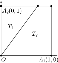
Figure 1: In the two-player case, player $1$ wins if and only if the random coordinate $\boldsymbol{t}$ falls into $T_{1}$.

For the two-player single-solution case, since there is only one solution, $t_{1}$ and $t_{2}$ are independently and uniformly distributed over $[0,1]$. Denote $\boldsymbol{t}=(t_{1},t_{2})$ and let $T_{1}$ be the set of $\boldsymbol{t}$ where player $1$ wins:

$$T_{1}=\{\boldsymbol{t}\in[0,1]^{2}:t_{1}/x_{1}\leq t_{2}/x_{2}\}.$$

Similarly, we can define $T_{2}$:

$$T_{2}=\{\boldsymbol{t}\in[0,1]^{2}:t_{2}/x_{2}\leq t_{1}/x_{1}\}.$$

Because $\boldsymbol{t}$ is uniformly distributed over $[0,1]^{2}$, $p_{1}=\int_{T_{1}}\mathrm{d}\boldsymbol{t}=\mathsf{area}(T_{1})$ equals to the area of set $T_{1}$ (see Figure 1). Suppose that $x_{1}\leq x_{2}$, then with some primary calculation, we know that the slope of the line separating $T_{1}$ and $T_{2}$ is $x_{2}/x_{1}$ and hence

$$p_{1}=\mathsf{area}(T_{1})=x_{1}/2x_{2},~{}p_{2}=\mathsf{area}(T_{2})=1-x_{1}/2x_{2},$$

which are not proportional to the computational power $x_{1}$ and $x_{2}$ (unless $x_{1}=x_{2}$).

3.2 $m$ players and a single solution

For the general $m$-player case, the winning probability of each player is summarized by the following theorem, where $\pi(z)$ and $\pi_{-i}(z)$ are defined to simplify the notations:

$$\pi(z)=\prod_{i=1}^{m}\left(1-\frac{x_{i}}{x_{m}}\cdot z\right),\quad\pi_{-i}(z)=\frac{\pi(z)}{1-\frac{x_{i}}{x_{m}}\cdot z}.$$

Theorem 1.

Suppose that $x_{1}\leq x_{2}\leq\cdots\leq x_{m}$, then the winning probability of player $i$ is:

$$p_{i}=\frac{x_{i}}{x_{m}}\int_{0}^{1}\pi_{-i}(z)\mathrm{d}z.$$

Proof.

Recall that

$$p_{i}=\Pr\left[t_{i}/x_{i}\leq\min_{j\neq i}t_{j}/x_{j}\right]=\Pr\bigg{[}\bigwedge_{j\neq i}t_{i}/x_{i}\leq t_{j}/x_{j}\bigg{]}.$$

Let $f_{i}(\cdot)$ be the probability density function of the random variable $t_{i}$, then

$$p_{i}=\int_{0}^{1}\Pr\bigg{[}\bigwedge_{j\neq i}t_{j}\geq\frac{t_{i}x_{j}}{x_{i}}\bigg{|}t_{i}=t\bigg{]}f_{i}(t)\mathrm{d}t.$$

Since the orders of the players enumerating through the candidates are independent, we have that

$$\Pr\bigg{[}\bigwedge_{j\neq i}t_{j}\geq\frac{t_{i}x_{j}}{x_{i}}\bigg{|}t_{i}=t\bigg{]}=\prod_{j\neq i}\Pr\left[t_{j}\geq\frac{tx_{j}}{x_{i}}\right].$$

In the meanwhile, note that $t_{1},\ldots,t_{m}$ are uniformly distributed, hence $f_{i}(t)=1$ and

$$\Pr\left[t_{j}\geq\frac{tx_{j}}{x_{i}}\right]=\max\left\{1-\frac{tx_{j}}{x_{i}},0\right\}.$$

Thus the production is zero for $t\geq x_{i}/x_{m}$, which implies

$$p_{i}=\int_{0}^{x_{i}/x_{m}}\prod_{j\neq i}\left(1-\frac{tx_{j}}{x_{i}}\right)\mathrm{d}t.$$

By substituting $t=x_{i}z/x_{m}$, we complete the proof

$$p_{i}=\frac{x_{i}}{x_{m}}\int_{0}^{1}\prod_{j\neq i}\left(1-\frac{x_{j}}{x_{m}}\cdot z\right)\mathrm{d}z=\frac{x_{i}}{x_{m}}\int_{0}^{1}\pi_{-i}(z)\mathrm{d}z.$$

∎

According to Theorem 1, the winning probabilities $p_{i}$ are proportional to the computational powers $x_{i}$ if and only if the integration $\int_{0}^{1}\pi_{-i}(z)\mathrm{d}z$ is a constant for all $1\leq i\leq m$, which in general is not true.

In particular, as we will show in Section 5, the observation above holds even when there are multiple solutions, i.e., $n>1$. Nevertheless, as $n$ goes to infinity, the winning probabilities will gradually get close to being proportional with respect to the computational powers.

However, the larger the player’s computational power is, the higher efficiency (winning probability divided by computational power) it achieves.

3.2.1 The Matthew Effect

The next theorem in fact indicates the Matthew effect in such systems: the player with higher computational power gets higher return (or higher probability to win) for each unit of their computational power, i.e., $p_{i}/x_{i}\leq p_{j}/x_{j}$.

Theorem 2 (The Matthew Effect).

If $x_{i}\leq x_{j}$, then $p_{i}/x_{i}\leq p_{j}/x_{j}$, where the equality is reached if and only if $x_{i}=x_{j}$.

If both of them invest all the rewards (such as bitcoins) they get to increase their future computational power, the ratio of $x_{j}/x_{i}$ will become larger and larger over time:

$\Delta x_{i}$ and $\Delta x_{j}$ are proportional to $p_{i}$ and $p_{j}$, respectively, hence

$$\Delta x_{i}/x_{i}\leq\Delta x_{j}/x_{j},\quad\Longrightarrow\quad(x_{i}+\Delta x_{i})/(x_{j}+\Delta x_{j})\leq x_{i}/x_{j}.$$

In other words, the player with the highest computational power in the system will gradually take a more and more fraction of the total computational power and eventually dominate the entire system.

Proof of Theorem 2.

To simplify the notations, write

$$\pi_{-ij}(z)=\frac{\pi(z)}{\big{(}1-\frac{x_{i}}{x_{m}}\cdot z\big{)}\big{(}1-\frac{x_{j}}{x_{m}}\cdot z\big{)}}.$$

Therefore, by $x_{i}\leq x_{j}\leq x_{m}$ and $\pi_{ij}(z)\geq 0$, we have that $\forall z\in[0,1]$,

$$\left(1-\frac{x_{j}}{x_{m}}\cdot z\right)\cdot\pi_{-ij}(z)\leq\left(1-\frac{x_{i}}{x_{m}}\cdot z\right)\cdot\pi_{-ij}(z).$$

Finally, using Theorem 1, we conclude that

$$\frac{p_{i}}{x_{i}}=\frac{1}{x_{m}}\int_{0}^{1}\left(1-\frac{x_{j}}{x_{m}}\cdot z\right)\cdot\pi_{-ij}(z)\mathrm{d}z\leq\frac{1}{x_{m}}\int_{0}^{1}\left(1-\frac{x_{i}}{x_{m}}\cdot z\right)\cdot\pi_{-ij}(z)\mathrm{d}z=\frac{p_{j}}{x_{j}}.$$

In particular, the equality is reached if and only if $x_{i}=x_{j}$. ∎

4 Pooling Incentives

In this section, we investigate the incentives of players to pool together assuming that the reward is split proportional to their computational powers. In particular, we identify a non-trivial Nash equilibrium of the following pool choosing game.

Definition (Pool choosing game).

Let $\mathcal{P}_{1},\ldots,\mathcal{P}_{m}$ be $m$ pools. The actions of each player is either to choose one from these $m$ pools (say $\mathcal{P}_{i}$) or to be independent (denoted as $\bot$). The utility of each player is the expected winning reward and if a pool wins, the reward is split proportional to its members’ computational powers.

In the practice of Bitcoin, there are many such pools. The pools have their own websites, cooperatively mining tools, and reward splitting policies. Usually, the pools always welcome miners to join so that they can attract more computational resources. In contrast, each individual miner can of course work by himself.

As a quick example, the action profile $(\mathcal{P}_{1},\ldots,\mathcal{P}_{1})$ results in a giant pool including everyone ($\{1,\ldots,m\}$) and the action profile $(\bot,\ldots,\bot)$ results in everyone being independent. Although trivial, the latter is a Nash equilibrium of the game. Because, for example, if player $i$ deviates, then the result is that only player $i$ in a pool and all others being independent. No difference.

The following theorem then identifies a non-trivial Nash equilibrium for two cases.

Theorem 3 (Nash Equilibrium).

Suppose that $x_{m}\geq x_{m-1}\geq\cdots\geq x_{1}$. If $x_{m}\leq x_{1}+\cdots+x_{m-1}$, then the action profile $(\mathcal{P}_{1},\ldots,\mathcal{P}_{1})$ is a Nash equilibrium, yielding a giant pool.

Otherwise, we have $x_{m}\geq x_{1}+\cdots+x_{m-1}$, and the action profile $(\mathcal{P}_{1},\ldots,\mathcal{P}_{1},\bot)$ is a Nash equilibrium, with player $m$ being independent and the others in one pool.

To prove this theorem, we first need to understand the conditions that a player has incentive to join a pool (or another player). With the theorems and lemmas in place, we prove Theorem 3 at the end of this section.

We also emphasize that the results in this section will later be generalized to the multiple-solution case in Section 5.

4.1 Incentive Analysis

First of all, an important and immediate observation for pooling is that pooling is always beneficial when taking the pool as a whole. Formally,

Observation .

A pool’s winning probability is no less than the sum of the winning probabilities of its members when they participate the computation contest separately.

This is easy to get by considering a “pseudo-pool” of the members, where they enumerate through the candidates in the same order as they do when participate the contest separately. Clearly, the winning probability of the “pseudo-pool” equals to the sum of the winning probabilities of the members working separately. Since the players in the “pseudo-pool” may repeatedly verify some of the candidates, the winning probability could be even higher if they simply skip those already verified by other members in the pool. In particular, this “higher” winning probability equals to the winning probability of the real pool by symmetry.

Theorem 4.

For any player $i$, pooling with another player with higher computational power than him is always beneficial.

Proof.

Consider a player $i$ pooling with another player $j$ with $x_{j}\geq x_{i}$. We use $p_{ij}$ to denote the winning probability of the pool. Then by Section 4.1, we have $p_{ij}\geq p_{i}+p_{j}$ and hence the reward of player $i$ from the pool is

$$p^{\prime}_{i}=\frac{x_{i}}{x_{i}+x_{j}}\cdot p_{ij}=\frac{p_{ij}}{1+x_{j}/x_{i}}\geq\frac{p_{i}+p_{i}}{1+x_{j}/x_{i}}.$$

Note that by Theorem 2, we have

$$p_{i}/x_{i}\leq p_{j}/x_{j}\quad\iff\quad x_{j}/x_{i}\leq p_{j}/p_{i}.$$

Therefore

$$p^{\prime}_{i}\geq\frac{p_{i}+p_{i}}{1+x_{j}/x_{i}}\geq\frac{p_{i}+p_{j}}{1+p_{j}/p_{i}}=p_{i}.$$

In other words, player $i$ gets more reward by pooling with player $j$. ∎

A direct consequence of this theorem is that a pool is stable against single deviation as long as the largest player’s computational power is no more than half of the computational power of the pool.

Corollary .

Any individual member of a pool has no incentive to leave if its computational power is no more than half of the pool’s computational power.

Proof.

Otherwise, once the player left the pool, he would have incentive to rejoin the pool by Theorem 4, a contradiction. ∎

In fact, the corollary asserts that any player (or pool) always has incentive to pool with a player (or pool) that has higher computational power than himself. In contrast, there would be a tradeoff for the player (or pool) being proposed:

• Pros: By pooling together, they form a larger pool, which by Theorem 2, has a higher efficiency in terms of computational power (i.e., higher ratio of reward divided by computational power).

• Cons: However, the player (or pool) with low computational power may actually takes more than he contributes. In this case, the total tradeoff for the player with high computational power could be negative and he would have incentive to be independent.

The following lemma then provides a sufficient condition where the tradeoff is positive.

Lemma .

If $x_{i}+x_{j}\leq x_{m}$, then both $i$ and $j$ will be better off in terms of the expected reward by pooling.

Proof.

Throughout the proof, we use the notations $\pi_{-ij}(z)$ (defined in the proof of Theorem 2) and $p_{ij}$ (the winning probability of the pool $\{i,j\}$).

Without loss of generality, suppose that $x_{i}\leq x_{j}\leq x_{m}$. Then by Theorem 4, player $i$ gets better off by pooling. In the rest of the proof, we show that player $j$ gets better off as well.

On one hand, according to the proportional allocation rule, the reward of player $j$ by pooling is $p^{\prime}_{j}=\frac{x_{j}}{x_{i}+x_{j}}\cdot p_{ij}$. Thinking the pool $\{i,j\}$ as a player with computational power $x_{i}+x_{j}$, then by Theorem 1,

$$p_{ij}=\frac{x_{i}+x_{j}}{x_{m}}\int_{0}^{1}\pi_{-ij}(z)\mathrm{d}z.$$

Hence

$$p^{\prime}_{j}=\frac{x_{j}}{x_{i}+x_{j}}\cdot p_{ij}=\frac{x_{j}}{x_{m}}\int_{0}^{1}\pi_{-ij}(z)\mathrm{d}z.$$

On the other hand, the reward of player $j$ without pooling is $p_{i}$, which by Theorem 1 is,

$$p_{j}=\frac{x_{j}}{x_{m}}\int_{0}^{1}\pi_{-j}(z)\mathrm{d}z.$$

Note that for any $z\in[0,1)$, since $x_{i}<x_{m}$ and $\pi_{-ij}(z)>0$,

$$\pi_{-ij}(z)>\left(1-\frac{x_{i}}{x_{m}}\cdot z\right)\pi_{-ij}(z)=\pi_{-j}(z).$$

Therefore,

$$p^{\prime}_{j}>p_{j}.$$

In other words, player $j$ gets strictly higher expected reward by pooling with player $i$. ∎

4.2 Equilibrium Analysis

Now we are ready to prove Theorem 3.

Theorem (Theorem 3 restate).

Suppose that $x_{m}\geq x_{m-1}\geq\cdots\geq x_{1}$. If $x_{m}\leq x_{1}+\cdots+x_{m-1}$, then the action profile $(\mathcal{P}_{1},\ldots,\mathcal{P}_{1})$ is a Nash equilibrium, yielding a giant pool.

Otherwise, we have $x_{m}\geq x_{1}+\cdots+x_{m-1}$, and the action profile $(\mathcal{P}_{1},\ldots,\mathcal{P}_{1},\bot)$ is a Nash equilibrium, with player $m$ being independent and the others in one pool.

Proof of Theorem 3.

The first case is a direct consequence of Section 4.1. Because none of them has computational power more than half of the pool, no player has incentive to deviate (leave the pool).

For the second case, we first show that player $m$ has no incentive to deviate (or equivalently, join pool $\mathcal{P}_{1}$).

We use $x_{-m}$ and $p_{-m}$ to denote the computational power and the winning probability of the pool $\{1,\ldots,m-1\}$, respectively. Since $x_{m}\geq x_{-m}$, by Theorem 2, $p_{m}/x_{m}\geq p_{-m}/x_{-m}$. Note that $p_{m}+p_{-m}=1$, hence $p_{-m}=1-p_{m}$. Then we have

$$\frac{p_{m}}{x_{m}}\geq\frac{1-p_{m}}{x_{-m}}\iff p_{m}\geq\frac{x_{m}}{x_{-m}+x_{m}},$$

where the right-hand-side is the reward of player $m$ if he joins the pool. In other words, if player $m$ deviates by joining pool $\mathcal{P}_{1}$, his winning probability will decreases.

Then we prove that any player $i\in\{1,\ldots,m-1\}$ has no incentive to deviate (or equivalently, leave pool $\mathcal{P}_{1}$).

To show this, we prove that player $i$ has incentive to join pool $\mathcal{P}^{\prime}_{1}$, when $\mathcal{P}^{\prime}_{1}=\{1,\ldots,i-1,i+1,\ldots,m-1\}$ and player $m$ chooses $\bot$. Thinking the pool $\mathcal{P}^{\prime}_{1}$ as a player with computational power $x^{\prime}=x_{1}+\cdots+x_{i-1}+x_{i+1}+\cdots+x_{m-1}$. Since $x_{i}+x^{\prime}\leq x_{m}$, then by Section 4.1, player $i$ has incentive to join pool $\mathcal{P}^{\prime}_{1}$. In other words, player $i$ gets (weakly) higher reward in pool $\mathcal{P}_{1}$ than being independent.

In summary, for the second case, no player has incentive to deviate, hence a Nash equilibrium. ∎

5 The Multiple-Solution Case

In this section, we first extend our results of single-solution cases to multiple-solution cases. Then we show that as the number of solutions goes to infinity, the winning probabilities become asymptotically proportional to the player computational powers. In particular, it means that the Matthew effect gets weaker as the number of solutions increases.

5.1 Generalization

We start with generalizing Theorem 1.

Theorem 5.

Suppose that $x_{1}\leq\cdots\leq x_{m}$, then the winning probability for player $i$ in the multiple-solution case is

$$p_{i}=\frac{x_{i}}{x_{m}}\int_{0}^{1}\pi_{-i}(z)\cdot\pi(z)^{n-1}\mathrm{d}z.$$

We omit the proof of this theorem but highlight the only two differences with the proof of Theorem 1. Both are because of the definition of $t_{i}$, the index of the first solution in player $i$’s sequence. Therefore, the probability density function of $t_{i}$ and the probability that $t_{j}\geq tx_{j}/x_{i}$ are different with those in the single-solution case:

$$f_{i}(t)=n(1-t)^{n-1},\Pr\left[t_{j}\geq\frac{tx_{j}}{x_{i}}\right]=\max\left\{1-\frac{tx_{j}}{x_{i}},0\right\}^{n}.$$

Then by substituting these two terms in the proof of Theorem 1, we get Theorem 5.

Based on Theorem 5, we claim that all previous results (except Theorem 1) also apply to multiple-solution cases:

Claim (Generalization).

Theorem 2 and Section 4.1 can be easily reproved for multiple-solution cases with Theorem 5. Based on this, Theorem 3, Section 4.1, Theorem 4, and Section 4.1 are automatically generalized because their proofs do not rely on the number of solutions.

5.2 Asymptotically Proportional Winning Probabilities

Consider the probability that the first solution comes after $t_{1},\ldots,t_{m}$ for each of the players. Since the distribution of each $t_{i}$ is independent, we have:

$$\Pr[\boldsymbol{\tau}\geq\boldsymbol{t}]=\prod_{i=1}^{m}\Pr[\tau_{i}\geq t_{i}]=\prod_{i=1}^{m}(1-t_{i})^{n},$$

hence its density function:

$$f(\boldsymbol{t})=\prod_{i=1}^{n}f_{i}(t_{i})=\prod_{i=1}^{n}\frac{\partial\left(1-t_{i}\right)^{n}}{\partial t_{i}}=n^{m}\prod_{i=1}^{m}(1-t_{i})^{n-1}.$$

Let $T_{i}$ be the set of $\boldsymbol{t}$ that player $i$ wins and $T=T_{1}\cup\cdots\cup T_{m}=[0,1]^{m}$. Then the winning probability of player $i$ is

$$p_{i}=\int_{\boldsymbol{t}\in T_{i}}f(\boldsymbol{t})\mathrm{d}\boldsymbol{t}.$$

Theorem 6 (Asymptotically Proportional).

For any fixed number of players, $m$, as the number of solutions, $n$, approaches to infinity,

$$p_{i}\longrightarrow\frac{x_{i}}{x_{1}+\cdots+x_{m}}.$$

In particular, the difference is vanishing in the order of $\widetilde{O}(n^{-1})$, i.e.,

$$\left|p_{i}-\frac{x_{i}}{x_{1}+\cdots+x_{m}}\right|=\widetilde{O}(n^{-1}).$$

The theorem could be directly derived based on the following Section 5.2 and Section 5.2.

We use $\rho_{i}(z)$ to denote the $(m-1)$-dimensional volume of set $\{\boldsymbol{t}\in T_{i}:t_{1}+\cdots+t_{m}=z\}$ and $\rho(z)=\rho_{1}(z)+\cdots+\rho_{m}(z)$.

Then Section 5.2 essentially means that $\boldsymbol{p}_{i}$ is asymptotically proportional to $\rho_{i}(1)$.

Lemma .

For any constant $m\ll n$,

$$p_{i}=\frac{\rho_{i}(1)}{\rho(1)}\cdot n^{m}\int_{0}^{n^{-1+\epsilon}}(1-z)^{n-1}\rho(z)\mathrm{d}z+\widetilde{O}(n^{-1}).$$

Furthermore, Section 5.2 indicates that $\rho_{i}(1)$ is proportional to the computational power of player $i$.

Lemma .

$$\frac{\rho_{i}(1)}{\rho(1)}=\frac{x_{i}}{x_{1}+\cdots+x_{m}}.$$

Proof of Theorem 6.

By Section 5.2 and Section 5.2. ∎

We dedicate the rest of this section to prove Section 5.2 and Section 5.2.

Proof idea of Section 5.2

The proof is done by a careful estimation of $p_{i}$ using a technique called the core-tail decomposition [Li and Yao,, 2013]. To estimate the probability, consider the core-tail decomposition of the set $T_{i}$, i.e., let

$$\mathsf{core}=\{\boldsymbol{t}:\bar{t}\leq\alpha\}\quad\text{and}\quad\mathsf{core}(T_{i})=\mathsf{core}\cap T_{i},$$

where $\bar{t}=t_{1}+\cdots+t_{m}$ and $\alpha>0$ is a parameter to be determined later. Similarly, define $\mathsf{tail}=[0,1]^{m}\setminus\mathsf{core}$ and $\mathsf{tail}(T_{i})=\mathsf{tail}\cap T_{i}$. Thus,

$$p_{i}=\int_{\mathsf{core}(T_{i})}f(\boldsymbol{t})\mathrm{d}\boldsymbol{t}+\int_{\mathsf{tail}(T_{i})}f(\boldsymbol{t})\mathrm{d}\boldsymbol{t}.$$ (1)

The following two lemmas would be helpful on simplifying the analysis.

Lemma .

Let $g(\boldsymbol{t})=n^{m}(1-\bar{t})^{n-1}$. If $\alpha<n^{-2/3}$, then

$$\int_{\mathsf{core}(T_{i})}f(\boldsymbol{t})\mathrm{d}\boldsymbol{t}=\int_{\mathsf{core}(T_{i})}g(\boldsymbol{t})\mathrm{d}\boldsymbol{t}+O(n^{m+1}\alpha^{m+2}).$$

Lemma .

$$\int_{\mathsf{tail}(T_{i})}f(\boldsymbol{t})\mathrm{d}\boldsymbol{t}\leq e^{-\alpha(n-1)+m\ln n}.$$

We postpone the proofs of these lemmas to Section 6, which are mainly elaborate treatments of the Taylor series.

Proof of Section 5.2.

Plugging Section 5.2 and Section 5.2 into (1), and letting $\alpha=\frac{(m+1)\ln n}{n-1}$, we have that,

$$p_{i}-\int_{\mathsf{core}(T_{i})}g(\boldsymbol{t})\mathrm{d}\boldsymbol{t}=O\left(n^{-1}(\ln n)^{m+2}\right)=\widetilde{O}(n^{-1}).$$

Hence we remain to show the following equation:

$$\int_{\mathsf{core}(T_{i})}g(\boldsymbol{t})\mathrm{d}\boldsymbol{t}=\frac{\rho_{i}(1)}{\rho(1)}\cdot n^{m}\int_{0}^{\alpha}(1-z)^{n-1}\rho(z)\mathrm{d}z,$$

or equivalently,

$$\!\int_{\mathsf{core}(T_{i})}(1-\bar{t})^{n-1}\mathrm{d}\boldsymbol{t}=\frac{\rho_{i}(1)}{\rho(1)}\int_{0}^{\alpha}(1-z)^{n-1}\rho(z)\mathrm{d}z. *$$ ()

First of all, note that the left-hand-side of ($*$ ‣ 5.2) could be rewritten as a double integration over $\mathsf{core}_{z}(T_{i})=\{\boldsymbol{t}\in\mathsf{core}(T_{i}):\bar{t}=z\}$ and then for $z$ from $0$ to $\alpha$:

$$\int_{\mathsf{core}(T_{i})}(1-\bar{t})^{n-1}\mathrm{d}\boldsymbol{t}=\int_{0}^{\alpha}\mathrm{d}z\int_{L}(1-z)^{n-1}\mathrm{d}\mathsf{core}_{z}(T_{i})=\int_{0}^{\alpha}(1-z)^{n-1}\mathrm{d}z\int_{L}\mathrm{d}\mathsf{core}_{z}(T_{i}),$$

where $\int_{L}\mathrm{d}S$ is the Lebesgue integration over a set $S$. In particular, $\int_{L}\mathrm{d}\mathsf{core}_{z}(T_{i})$ is the $(m-1)$-dimensional volume of the set $\mathsf{core}_{z}(T_{i})$, denoted as $\rho_{i}(z)$.

Then consider the ratio between $\rho_{i}(z)$ and the volume of set $\mathsf{core}_{z}(T)$, $\rho(z)$. Since both $\mathsf{core}(T_{i})$ and $\mathsf{core}(T)$ are the intersections of the $\mathsf{core}$ and positive cones in $\mathbb{R}^{m}$, hence $\rho_{i}(z)$ and $\rho(z)$ must be proportional to $z^{m-1}$ accordingly:

$$\rho_{i}(z)=z^{m-1}\rho_{i}(1),\quad\rho(z)=z^{m-1}\rho(1).$$

Finally, we conclude that

$$\int_{L}\mathrm{d}\mathsf{core}_{z}(T_{i})=\rho_{i}(z)=\frac{\rho_{i}(1)}{\rho(1)}\cdot\rho(z),$$

which then directly implies ($*$ ‣ 5.2). ∎

Proof idea of Section 5.2

To smoothly proceed the analysis, we will start with the cases of $m=2$ and $m=3$.

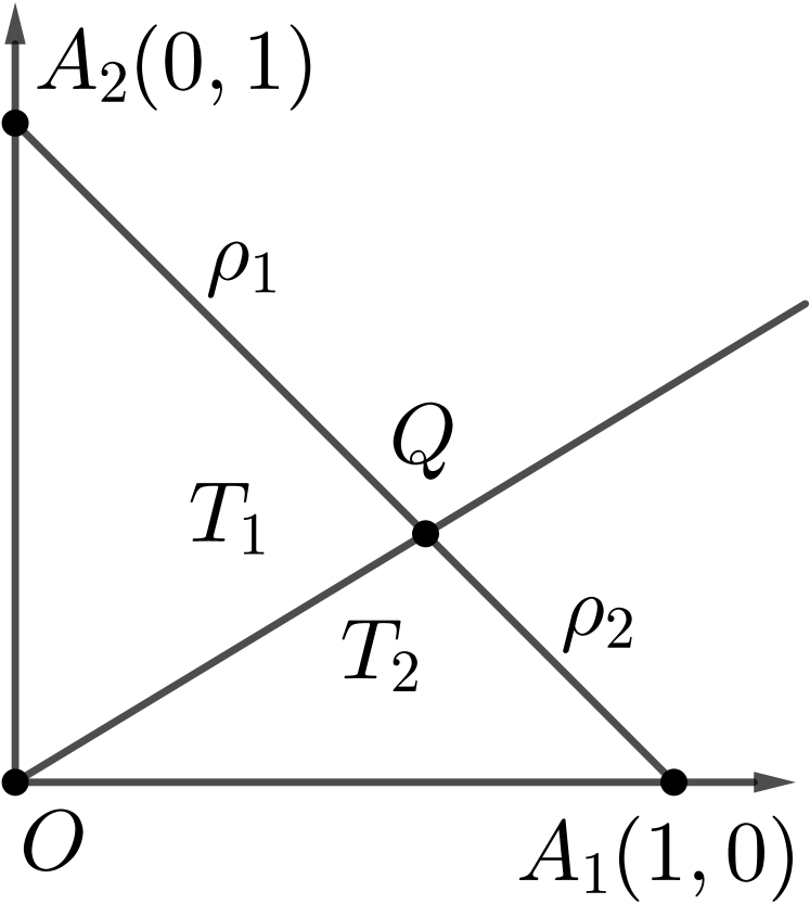
(a) The two-player case.

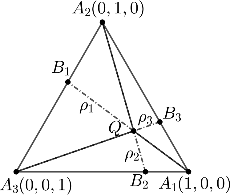
(b) The three-player case.

.

Figure 2: Simplexes for two-player and three-player cases.

For the two-player case (see 2(a)), by definition,

$$T_{1}=\{\boldsymbol{t}\in[0,1]^{2}:t_{1}/x_{1}\leq t_{2}/x_{2}\},$$

$$T_{2}=\{\boldsymbol{t}\in[0,1]^{2}:t_{2}/x_{2}\leq t_{1}/x_{1}\}.$$

Therefore, the formula of the hyperplane (in fact a line in the $2$-dimensional case) separating $T_{1}$ and $T_{2}$ is $t_{1}/x_{1}=t_{2}/x_{2}$ and $Q$ is the intersection of this line and the simplex $A_{1}A_{2}$. In particular, the $1$-dimensional volume of the set $\{\boldsymbol{t}\in T_{1}:\bar{t}=1\}$ is exactly the length of the line segment $QA_{2}$, which equals to $\rho_{1}(1)=\sqrt{2}x_{1}/(x_{1}+x_{2})$. Similarly, we get $\rho_{2}(1)=\sqrt{2}x_{2}/(x_{1}+x_{2})$.

For the three-player case (see 2(b)), by definition,

$$T_{1}=\{\boldsymbol{t}\in[0,1]^{3}:t_{1}/x_{1}\leq t_{2}/x_{2},t_{1}/x_{1}\leq t_{3}/x_{3}\},$$

$$T_{2}=\{\boldsymbol{t}\in[0,1]^{3}:t_{2}/x_{2}\leq t_{1}/x_{1},t_{2}/x_{2}\leq t_{3}/x_{3}\},$$

$$T_{3}=\{\boldsymbol{t}\in[0,1]^{3}:t_{3}/x_{3}\leq t_{1}/x_{1},t_{3}/x_{3}\leq t_{2}/x_{2}\}.$$

In this case, there are three hyperplanes separating $T_{1}$, $T_{2}$, and $T_{3}$: $t_{1}/x_{1}=t_{2}/x_{2}$, $t_{2}/x_{2}=t_{3}/x_{3}$, and $t_{3}/x_{3}=t_{1}/x_{1}$. Note that the intersection of the three hyperplanes is a line, $t_{1}/x_{1}=t_{2}/x_{2}=t_{3}/x_{3}$, which then intersects with the simplex $A_{1}A_{2}A_{3}=\{\boldsymbol{t}:t_{1}+t_{2}+t_{3}=1\}$ at a point $Q$.

Therefore, the $2$-dimensional volumes (or areas) $\rho_{1}(1)$, $\rho_{2}(1)$, and $\rho_{3}(1)$ are exactly the areas of triangles $\triangle QA_{2}A_{3}$, $\triangle A_{1}QA_{3}$, and $\triangle A_{1}A_{2}Q$, respectively. Note that $A_{1}A_{2}A_{3}$ is a regular $2$-simplex, hence $A_{2}A_{3}=A_{3}A_{1}=A_{1}A_{2}$. Thus the ratios between the areas of the triangles equal to the ratios between the heights of the triangles, because their bases ($A_{2}A_{3}$, $A_{3}A_{1}$, $A_{1}A_{2}$) are of the same length.

We conclude that

$$\frac{\rho_{1}(1)}{\rho_{2}(1)}=\frac{d(Q,A_{2}A_{3})}{d(Q,A_{3}A_{1})},\frac{\rho_{1}(1)}{\rho_{3}(1)}=\frac{d(Q,A_{2}A_{3})}{d(Q,A_{1}A_{2})},$$

where $d$ denotes the distance between a point and a line.

In the meanwhile, recall that the coordinate of point $Q$ is:

$$\left(\frac{x_{1}}{x_{1}+x_{2}+x_{3}},\frac{x_{2}}{x_{1}+x_{2}+x_{3}},\frac{x_{3}}{x_{1}+x_{2}+x_{3}}\right),$$

and with some primary calculation, we know that

$$\frac{d(Q,A_{2}A_{3})}{d(Q,A_{3}A_{1})}=\frac{x_{1}}{x_{2}}\quad\text{and}\quad\frac{d(Q,A_{2}A_{3})}{d(Q,A_{1}A_{2})}=\frac{x_{1}}{x_{3}}.$$

In other words, $\rho_{i}(1)/\rho(1)=x_{i}/(x_{1}+x_{2}+x_{3})$.

Finally, we generalize the observations above to get the proof.

Proof of Section 5.2.

By the definition, $T_{1},\ldots,T_{m}$ are separated by ${m\choose 2}$ hyperplanes:

$$\forall i\neq j,t_{i}/x_{i}=t_{j}/x_{j}.$$

In particular, the intersection of them is a line and the line intersects the $(m-1)$-simplex $A_{1}\cdots A_{m}$ at a unique point $Q$, whose coordinate is:

$$Q:\left(\frac{x_{1}}{x_{1}+\cdots+x_{m}},\ldots,\frac{x_{m}}{x_{1}+\cdots+x_{m}}\right).$$

In the meanwhile, note that for each $i\in[m]$, point $A_{j}\in T_{i}$ for all $j\neq i$. Therefore, the set $\{\boldsymbol{t}\in T_{i}:\bar{t}=1\}$ is a $(m-1)$-simplex, $A_{1}\cdots A_{i-1}QA_{i+1}\cdots A_{m}$ and its volume is proportional to the $(m-2)$-dimensional volume of its base $A_{1}\cdots A_{i-1}A_{i+1}\cdots A_{m}$ times its height (the distance between point $Q$ and the base).

Because $A_{1}\cdots A_{m}$ is a regular $(m-1)$-simplex, the volumes of the bases for each $i$ are the same. Therefore, $\rho_{i}(1)/\rho_{j}(1)$ equals to the ratios between the distances from $Q$ to the corresponding bases. Based on the coordinate of $Q$, we conclude that the ratio equals to $x_{i}/x_{j}$. In other words,

$$\frac{\rho_{i}(1)}{\rho(1)}=\frac{\rho_{i}(1)}{\rho_{1}(1)+\cdots+\rho_{m}(1)}=\frac{x_{i}}{x_{1}+\cdots+x_{m}}.$$

∎

6 Missing Proofs

The following technical lemma is repeatedly used in the proofs.

Lemma .

For all $x\in\mathbb{R}$, $e^{x}\geq 1+x$.

Proof of Section 5.2.

For the $\mathsf{core}$ part, because $\bar{t}<\alpha<n^{-2/3}$,

$$\prod_{i=1}^{m}(1-t_{i})=1-\sum_{i}t_{i}+\sum_{i\neq j}t_{i}t_{j}+\cdots=1-\bar{t}+O(\bar{t}^{2}),$$

$$\prod_{i=1}^{m}(1-t_{i})^{n-1}=(1-\bar{t})^{n-1}\left(1+\frac{O(\bar{t}^{2})}{1-\bar{t}}\right)^{n-1}.$$

Since $n\bar{t}^{2}\leq n\alpha^{2}<n^{-1/3}$, then by Section 6 and Taylor’s expansion of $e^{x}$ at $0$,

$$\prod_{i=1}^{m}(1-t_{i})^{n-1}\leq(1-\bar{t})^{n-1}e^{\frac{O(\bar{t}^{2})}{1-\bar{t}}\cdot(n-1)}={}(1-\bar{t})^{n-1}\cdot\left(1+\frac{O(\bar{t}^{2})(n-1)}{1-\bar{t}}+O(n^{2}\bar{t}^{4})\right)={}(1-\bar{t})^{n-1}+O(n\bar{t}^{2}).$$

Thus

$$\int_{\mathsf{core}(T_{i})}f(\boldsymbol{t})\mathrm{d}\boldsymbol{t}\leq\int_{\mathsf{core}(T_{i})}n^{m}\left((1-\bar{t})^{n-1}+O(n\bar{t}^{2})\right)\mathrm{d}\boldsymbol{t},$$

where

$$\int_{\mathsf{core}(T_{i})}n^{m}\cdot O(n\bar{t}^{2})\mathrm{d}\boldsymbol{t}\leq n^{m+1}\int_{\mathsf{core}}O(\bar{t}^{2})\mathrm{d}t.$$

Consider rewrite the right-hand-side as a double integration over $\mathsf{core}_{z}=\{\boldsymbol{t}\in\mathsf{core}:\bar{t}=z\}$ and then for $z$ from $0$ to $\alpha$:

$$\int_{\mathsf{core}}O(\bar{t}^{2})\mathrm{d}t=\int_{0}^{\alpha}O(z^{2})\mathrm{d}z\int_{L}\mathrm{d}{\mathsf{core}_{z}}$$

Note that $\int_{L}\mathrm{d}{\mathsf{core}_{z}}$ is the Lebesgue integration over the set $\mathsf{core}_{z}$ and hence equals to its $(m-1)$-dimensional volume, which is $\rho(z)=\frac{\sqrt{m}}{(m-1)!}\cdot z^{m-1}$ [Stein,, 1966]. Therefore,

$$\int_{\mathsf{core}}O(\bar{t}^{2})\mathrm{d}t=\int_{0}^{\alpha}O(z^{2})\cdot z^{m-1}\mathrm{d}z=O(\alpha^{m+2}).$$

That is

$$\int_{\mathsf{core}(T_{i})}n^{m}\cdot O(n\bar{t}^{2})\mathrm{d}\boldsymbol{t}\leq O(n^{m+1}\alpha^{m+2}).$$

In summary,

$$\int_{\mathsf{core}(T_{i})}f(\boldsymbol{t})\mathrm{d}\boldsymbol{t}=\int_{\mathsf{core}(T_{i})}g(\boldsymbol{t})\mathrm{d}\boldsymbol{t}+O(n^{m+1}\alpha^{m+2}).$$

∎

Proof of Section 5.2.

For the $\mathsf{tail}$ part, according to the inequality of arithmetic and geometric means,

$$\prod_{i=1}^{m}(1-t_{i})\leq(1-\bar{t}/m)^{m},$$

then by Section 6 and $\bar{t}\geq\alpha$,

$$\prod_{i=1}^{m}(1-t_{i})^{n-1}\leq(1-\bar{t}/m)^{m(n-1)}\leq e^{-\bar{t}(n-1)}\leq e^{-\alpha(n-1)}.$$

Therefore, $f(\boldsymbol{t})\leq n^{m}e^{-\alpha(n-1)}=e^{-\alpha(n-1)+m\ln n}$. Also note that $\int_{\mathsf{tail}}\mathrm{d}\boldsymbol{t}$ is the volume of $\mathsf{tail}$, which is less than $1$, hence

$$\int_{\mathsf{tail}(T_{i})}f(\boldsymbol{t})\mathrm{d}\boldsymbol{t}\leq e^{-\alpha(n-1)+m\ln n}\int_{\mathsf{tail}}\mathrm{d}\boldsymbol{t}\leq e^{-\alpha(n-1)+m\ln n}.$$

∎

References

- Antonopoulos, [2014] Antonopoulos, A. M. (2014). Mastering Bitcoin: unlocking digital cryptocurrencies. ” O’Reilly Media, Inc.”.
- Bloch, [1996] Bloch, F. (1996). Sequential formation of coalitions in games with externalities and fixed payoff division. Games and Economic Behavior, 14(1):90–123.
- Canbolat et al., [2012] Canbolat, P. G., Golany, B., Mund, I., and Rothblum, U. G. (2012). A stochastic competitive r&d race where “winner takes all”. Operations Research, 60(3):700–715.
- Cooper et al., [2010] Cooper, S., Khatib, F., Treuille, A., Barbero, J., Lee, J., Beenen, M., Leaver-Fay, A., Baker, D., Popović, Z., et al. (2010). Predicting protein structures with a multiplayer online game. Nature, 466(7307):756.
- Eyal, [2015] Eyal, I. (2015). The miner’s dilemma. In Security and Privacy (SP), 2015 IEEE Symposium on, pages 89–103. IEEE.
- Eyal and Sirer, [2018] Eyal, I. and Sirer, E. G. (2018). Majority is not enough: Bitcoin mining is vulnerable. Communications of the ACM, 61(7):95–102.
- Fisch et al., [2017] Fisch, B., Pass, R., and Shelat, A. (2017). Socially optimal mining pools. In International Conference on Web and Internet Economics, pages 205–218. Springer.
- Harris and Vickers, [1987] Harris, C. and Vickers, J. (1987). Racing with uncertainty. The Review of Economic Studies, 54(1):1–21.
- Horowitz et al., [2016] Horowitz, S., Koepnick, B., Martin, R., Tymieniecki, A., Winburn, A. A., Cooper, S., Flatten, J., Rogawski, D. S., Koropatkin, N. M., Hailu, T. T., et al. (2016). Determining crystal structures through crowdsourcing and coursework. Nature communications, 7:12549.
- Kiayias et al., [2016] Kiayias, A., Koutsoupias, E., Kyropoulou, M., and Tselekounis, Y. (2016). Blockchain mining games. In Proceedings of the 2016 ACM Conference on Economics and Computation, pages 365–382. ACM.
- Li and Yao, [2013] Li, X. and Yao, A. C.-C. (2013). On revenue maximization for selling multiple independently distributed items. Proceedings of the National Academy of Sciences, 110(28):11232–11237.
- Liu et al., [2018] Liu, X., Wang, W., Niyato, D., Zhao, N., and Wang, P. (2018). Evolutionary game for mining pool selection in blockchain networks. IEEE Wireless Communications Letters.
- Mnih et al., [2015] Mnih, V., Kavukcuoglu, K., Silver, D., Rusu, A. A., Veness, J., Bellemare, M. G., Graves, A., Riedmiller, M., Fidjeland, A. K., Ostrovski, G., et al. (2015). Human-level control through deep reinforcement learning. Nature, 518(7540):529.
- Nakamoto, [2008] Nakamoto, S. (2008). Bitcoin: A peer-to-peer electronic cash system.
- Rosenfeld, [2011] Rosenfeld, M. (2011). Analysis of bitcoin pooled mining reward systems. arXiv preprint arXiv:1112.4980.
- [16] Silver, D., Hubert, T., Schrittwieser, J., Antonoglou, I., Lai, M., Guez, A., Lanctot, M., Sifre, L., Kumaran, D., Graepel, T., et al. (2017a). Mastering chess and shogi by self-play with a general reinforcement learning algorithm. arXiv preprint arXiv:1712.01815.
- [17] Silver, D., Schrittwieser, J., Simonyan, K., Antonoglou, I., Huang, A., Guez, A., Hubert, T., Baker, L., Lai, M., Bolton, A., et al. (2017b). Mastering the game of go without human knowledge. Nature, 550(7676):354.
- Stein, [1966] Stein, P. (1966). A note on the volume of a simplex. The American Mathematical Monthly, 73(3):299–301.
- Tschorsch and Scheuermann, [2016] Tschorsch, F. and Scheuermann, B. (2016). Bitcoin and beyond: A technical survey on decentralized digital currencies. IEEE Communications Surveys & Tutorials, 18(3):2084–2123.