Coulomb-promoted spintromechanics in magnetic shuttle devices

Abstract

Exchange forces on the movable dot (”shuttle”) in a magnetic shuttle device depend on the parity of the number of shuttling electrons. The performance of such a device can therefore be tuned by changing the strength $U$ of Coulomb correlations to block or unblock parity fluctuations. We show that by increasing $U$ the spintro-mechanics of the device crosses over, at $U=U_{c}(T)$, from a mechanically stable regime to a regime of spin-induced shuttle instabilities. This is due to enhanced spin-dependent mechanical forces as parity fluctuations are reduced by a Coulomb blockade of tunneling and demonstrates that single-electron manipulation of single-spin controlled nano-mechanics is possible.

Single-electronics devoret and spintronics zutic are mesoscopic research areas related to two fundamental properties of electrons: their charge and their spin. Strong Coulomb correlations and quantum coherent electron spin dynamics in nanometer-size conductors make them candidates for future device applications. In this context it is interesting to explore the interplay between spin- and charge degrees of freedom on the nanometer length scale.

Tunneling injection of electrons into a nanoconductor is an obvious way to control the amount of both charge and spin accumulated in a nanometer scale spatial domain. However, in contrast to the amount of electric charge the amount of electron spin that can be accumulated by this process is limited. This is because while electrons with different spin projections can be injected into the conductor, the net spin accumulated depends — assuming a spin-degenerate electronic spectrum — on the parity of the number of injected electrons. The net accumulated spin, at equilibrium, is at most equal to a single electron spin and this occurs only for an odd number of injected electrons. Quantum fluctuations of the electron number destroy all effects originating from parity, thus prohibiting the tunneling accumulation of a finite average amount of spin. By suppressing these parity fluctuations the Coulomb blockade phenomenon enhances the probability for a finite spin to be accumulated. This opens an intriguing possibility to use the interplay between single-electronic and spintronic properties for designing the functionality of nanoconductors.

Spintromechanics pulkin relies on a coupling between mechanical degrees of freedom and the electron spin in magnetic nanoelectromechanical (NEM) devices zant ; mceuen (see e.g. reviews Ref. blencowe, , Ref. aldridge, ). The coupling is due to the magnetic exchange interaction between spins accumulated in the movable part of the NEM device (a metal grain or molecule here called a “dot”) and the magnetization in the leads. This makes spintromechanical phenomena an important tool for probing the spin accumulated in a nanoconductor. One can therefore expect a prominent role for Coulomb correlations in the spintromechanical performance of magnetic NEM devices.

Below we consider the interplay between spintromechanical and single-electron performances of a magnetic NEM system, taking the magnetic shuttle device ( see, e.g., Refs. erbe, , pistolesi, ) as an example. We demonstrate that a dramatic change of the mechanical behavior of the shuttle device can be induced by using a gate to increase the electron-number (parity) fluctuations in the dot, corresponding to a lifting of the Coulomb blockade of tunneling. As a consequence of the related increase of the fluctuations of the spin-dependent mechanical force on the dot the shuttle instability of the magnetic NEM device, predicted to occur in the absence of parity fluctuations in Ref. kulinich, , is suppressed.

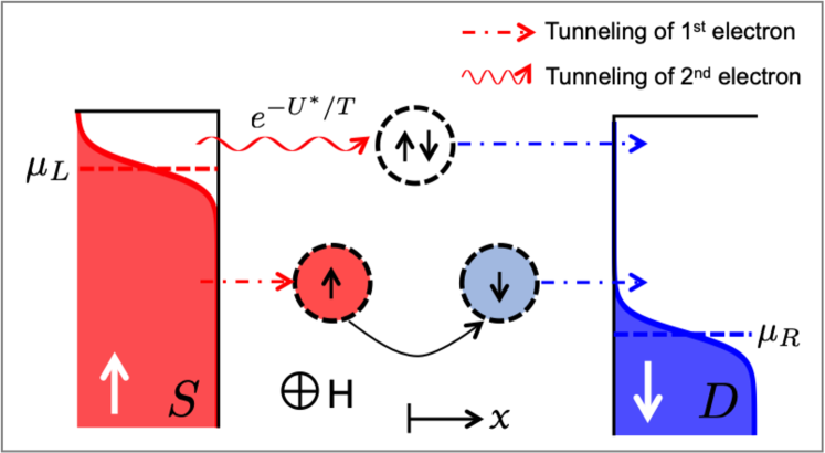
Figure 1: Mechanism of Coulomb-promoted spintromechanics: A spin-up electron loaded to the shuttle from the fully polarized source electrode ($S$) interacts with the magnetizations in the leads to create a magnetic exchange force that attracts the dot to the source (red dot). An external magnetic field “rotates” the spin into a spin-down state, thereby reversing the sign of the exchange force so that the shuttle is pushed towards the drain ($D$) (blue dot). In the case of a full Coulomb blockade ($U^{\ast}\rightarrow\infty$, see text), which prevents double occupation, the shuttle becomes mechanically active and energy is pumped into the mechanical shuttle vibrations. With a partial Coulomb blockade double occupation of the shuttle occurs with probability $\exp(-U^{\ast}/T)$, where $T$ is the temperature, leading to electron parity fluctuations, which are detrimental to the energy pumping mechanism.

A typical magnetic shuttle device comprises two magnetic metallic electrodes, which form a standard tunnel junction, while a movable small conductor (dot) is trapped (e.g., by van der Waals forces) in the tunneling region of the device. By biasing the device by a voltage difference or a temperature gradient, a flow of electrons is induced between the magnetic electrodes with the possibility for extra electrons to be resident in the dot. In a steady state, the electric charge and net electron spin accumulated in the dot interact with the electric field (caused by the bias voltage) and with the magnetic (exchange) forces (caused by the interaction of the quantum dot spin with the magnetizations of the leads). This is how a coupling between mechanical vibrations and electron tunneling through the device is induced (see supplementary material).

We model the quantum dot by a single spin-degenerate electron level and assume that the leads are fully spin-polarized half-metals with anti-parallel magnetizations. In Fig. 1 different tunneling and spin-flip events, which modify the electronic population in the dot, are specified. Tunneling events, leading to a singly and a doubly occupied dot, are discriminated by the extra Coulomb energy cost $U$ for the dot to be doubly occupied. If the energy of the singly occupied dot is $\varepsilon_{0}$, then the activation energy $U^{\ast}$ required for a second electron to tunnel to the dot is

$$U^{\ast}=U+\varepsilon_{0}-\mu_{L},$$ (1)

where $\mu_{L}$ is the chemical potential in the left lead.

Let us first consider the limit of strong Coulomb correlations ($U\to\infty$), in which case double occupation of the dot is prohibited. Then, we note that an important requirement for the proper operation of a magnetic shuttle device is that an external magnetic field is applied perpendicular to the magnetizations of the leads. This field makes it possible for a spin-up electron injected into the dot from the source electrode, to flip its spin, as indicated in Fig. 1. The resulting change of spin orientation enables the exchange force to push the dot away from the source towards the drain electrode, into which the extra electron tunnels, thus causing the empty dot to move back to the source electrode. This is the mechanism by which an electron flow through the device can generate mechanical oscillations and, under certain conditions, the spin-induced shuttle instability predicted in Ref. kulinich, (where it was assumed that no more than one electron occupies the dot at any time).

Next we explore the consequences of our ability to vary the effect of the Coulomb correlations by increasing the temperature or by gating the device. To that end we consider strong Coulomb blockade regime, $U^{\ast}\gg T$, where $T$ is the temperature, in which case there is a small probability for a spin-up second electron to tunnel into the dot already occupied by a spin-down electron. Three electronic configurations on the dot are now possible. Two of them, the dot singly occupied by a spin-up electron — prevented to tunnel into the drain since it has only spin-down states — and the dot doubly occupied by one spin-up and one spin-down electron, are “mechanically inactive” in the sense that no net work is done during one oscillation period against the exchange force. Only the third configuration, the dot singly occupied by a spin-down electron, is mechanically active, which enables energy, accumulated by electrons, to be transferred into mechanical vibration energy.

The functionality of the magnetic shuttle device is determined by the coupling of three different degrees of freedom. Those are related to: (i) the spatial tunneling motion of electrons between the leads via the quantum dot, (ii) the rigid mechanical motion of the movable dot, which affects electron tunneling probabilities, and (iii) the electron spin dynamics, which influences the mechanical motion of the dot through the exchange force, acting on the quantum dot.

Referring to Fig. 1, the classical nanomechanics of the shuttle vibrations can be described by Newton’s equation for the oscillator with a spin- and displacement-dependent “external” exchange force ilinskaya ,

$$m\ddot{x}+m\omega^{2}x=-\frac{\alpha}{2}\left[\rho_{\uparrow}\{x(t)\}-\rho_{\downarrow}\{x(t)\}\right].$$ (2)

Here the coefficient $\alpha$ is the magnitude of the exchange force per unit spin experienced by a shuttle, situated in the middle of the gap ($x$=0) between the oppositely magnetized leads, where the exchange energy $J(x)=J_{L}(x)-J_{R}(x)\simeq-\alpha x$ [we consider a magnetically symmetric contact, $J_{L}(0)=J_{R}(0)\equiv J$]; $J$ is the strength of exchange interaction, $m$ is the mass of the dot and $\omega$ is the angular frequency of the mechanical vibrations of the dot.

The exchange force on the right-hand side of Eq. (2) is proportional to the displacement-dependent amount of spin accumulated in the dot, which depends on the difference between the probabilities $\rho_{\uparrow(\downarrow)}\{x(t)\}$ for the dot to be singly occupied by a spin-up (down) electron. These probabilities are solutions to a complex kinetic problem for the quantum evolution of the electron density operator $\hat{\rho}$, describing the interplay between mechanical vibrations, coherent spin dynamics in the exchange and external magnetic fields and incoherent tunneling of electrons SM .

The corresponding equations can be derived to lowest order in the tunneling probabilities by following the procedure used in Ref. ilinskaya, . In this approach electrons in the leads are described by equilibrium distribution functions and therefore all electronic degrees of freedom in the leads are easily averaged out. The electron distribution in the dot is described using the Fock representation. In this representation, four eigenstates, corresponding to the empty dot, $|0\rangle$, to the dot, singly occupied by a spin-up (down) electron, $\mid\uparrow\rangle$ ($\mid\downarrow\rangle$), and to the doubly occupied dot, $|2\rangle$, form a complete Hilbert space for the single-level quantum dot. The matrix elements of the density operator form a $6$-vector with components: $\rho_{0}\equiv\langle 0|\hat{\rho}_{d}|0\rangle$, $\rho_{\uparrow}\equiv\langle\uparrow|\hat{\rho}_{d}|\uparrow\rangle$, $\rho_{\downarrow}\equiv\langle\downarrow|\hat{\rho}_{d}|\downarrow\rangle$, $\rho_{\uparrow\downarrow}=\rho_{\downarrow\uparrow}^{\ast}\equiv\langle\uparrow|\hat{\rho}_{d}|\downarrow\rangle$, $\rho_{2}\equiv\langle 2|\hat{\rho}_{d}|2\rangle$. Here $\rho_{0}$ ($\rho_{2}$) is the probability for the dot to be empty (doubly occupied), while the other matrix elements correspond to a singly occupied dot (including the non-diagonal components $\rho_{\uparrow\downarrow}$, $\rho_{\downarrow\uparrow}$). The number of independent variables can be reduced by one using the normalization condition $\rho_{0}+\rho_{\uparrow}+\rho_{\downarrow}+\rho_{2}=1$. All matrix elements experience two types of dynamical evolution: (i) electron tunneling events, described by classical “collision” integrals, and (ii) quantum coherent spin evolution in response to the exchange field and to the external magnetic field $H$. In order to study the mechanical motion of the quantum dot, we are interested in the dynamics of the ”spin active” linear combination of distribution functions, $\rho_{\uparrow}-\rho_{\downarrow}$. It is easy to show that the symmetric spin-neutral quantities $R_{0}=\rho_{0}+\rho_{2}$ and $\rho_{\uparrow}+\rho_{\downarrow}=1-R_{0}$ are decoupled from the equations for the four other linear combinations: $R_{1}=\rho_{0}-\rho_{2}$, $R_{2}=\rho_{\uparrow}-\rho_{\downarrow}$, $R_{3}=-i(\rho_{\uparrow\downarrow}-\rho_{\uparrow\downarrow}^{\ast})$, and $R_{4}=\rho_{\uparrow\downarrow}+\rho_{\uparrow\downarrow}^{\ast}$. It follows that the set of equations, describing tunneling and spin evolution of the density operator, can be written in the compact form SM

$$\frac{d\overrightarrow{R}}{dt}=\left(\hat{A}_{\Gamma}+\hat{A}_{H}+\hat{A}_{J}\right)\overrightarrow{R}+\overrightarrow{B}.$$ (3)

Here the matrices $\hat{A}_{\Gamma,H,J}$, which describe the dynamics, caused by tunneling ($\hat{A}_{\Gamma}$), spin evolution in the external magnetic field ($\hat{A}_{H}$), and spin evolution due to the exchange interaction ($\hat{A}_{J}$), and the “source term” $\overrightarrow{B}$ are defined by Eqs. (25)-(31) of Ref. SM, .

Equations (2) and (29) form a closed set of equations, describing the spintromechanics of the magnetic shuttle device. Being nonlinear, they can in a general case only be solved numerically. Whether a nanomechanical instability can be triggered by injecting an electron current into the device is the most important question to address. The answer can be obtained by linearizing Eqs. (2) and (29) with respect to small mechanical dot displacements and by finding the condition for the exponential growth (in time) of their amplitude. Having in mind the above qualitative analysis, one expects that the criterion for a mechanical instability crucially depends on the strength of the Coulomb charging energy $U$. In the Coulomb blockade regime, $U^{\ast}\gg T$, the existence of a shuttle instability for such a system was predicted in Ref. ilinskaya, . The solution of the linearized Eqs. (2) and (29) can also be found in the opposite limit of non-interacting electrons, $U=0$, for the case of a symmetric junction $\Gamma_{L}=\Gamma_{R}\equiv\Gamma$ SM ($\Gamma_{L,R}$ are partial dot tunneling widths). In this case we have shown [SM, ] that the exchange interaction, caused by the electron spin, results in a positive imaginary part of the renormalized angular frequency $\Omega$ of the mechanical vibrations. This corresponds to an exponential time decay of the amplitude of mechanical vibrations [$x(t)\sim\exp(i\Omega t)]$]. Straightforward calculations SM yield for the rate of change, $r$, of the amplitude of the nanomechanical vibrations at $U=0$

$$r=-\text{Im}\Omega(h) = -\frac{\alpha^{2}}{16m}\sum_{j=L,R}\frac{f_{j}(\varepsilon_{0}-h)-f_{j}(\varepsilon_{0}+h)}{h}\times$$ (4)

$$\times \frac{\Gamma(\Gamma^{2}+\omega^{2}+4h^{2})}{(\Gamma^{2}-\omega^{2}+4h^{2})^{2}+4\omega^{2}\Gamma^{2}}.$$

Here $\hbar=1$, $h=g\mu_{B}H/2$ is the external magnetic field in energy units ($\mu_{B}$ is the Bohr magneton, $g$ is the gyromagnetic ratio). The negative value of the rate is evident from the monotonic decay of the Fermi distribution function, $f_{j}(\epsilon)=1/\left\{\exp[(\epsilon-\mu_{j})/T_{j}+1]\right\}$, determined by chemical potentials $\mu_{j}$ and temperatures $T_{j}$ in the leads $j=L,R$. In the numerical analysis below we assume that the temperatures in the leads are the same, $T_{L}=T_{R}=T$, and in the unbiased device $\mu_{L}=\mu_{R}=\varepsilon_{F}$.

The result, presented in Eq. (4), suggests that a crucial change in spintromechanical performance occurs when Coulomb correlations are tuned. While increasing $U$ from zero, one stimulates a performance, which eventually results in the occurrence of a nanomechanical instability at a certain critical value of $U=U_{c}$.

The temperature-dependent crossover from a mechanically stable regime, where spontaneous dot fluctuations are damped out, to a shuttling regime, where they are amplified, occurs at $U^{\ast}_{c}$ when the ratio of double to single spin-down occupations reaches a critical value $\rho_{2}/\rho_{\downarrow}=n_{c}$. The critical value $U^{\ast}_{c}$ and $n_{c}$ are related by a simple steady state relation $\Gamma_{L}\exp(-U^{\ast}/T)=n_{c}\Gamma_{R}$ (here we neglect electron backflow and we omit all terms proportional to small magnetic field). The critical activation energy reads

$$U_{c}^{\ast}\simeq T\ln\left(\frac{\Gamma_{L}}{n_{c}\Gamma_{R}}\right),$$ (5)

corresponding to a linear dependence of the critical Coulomb energy on temperature and a slight (logarithmic) decrease of the slope with an increase of the “asymmetry parameter“ $\gamma=\Gamma_{R}/\Gamma_{L}$ of the shuttle device.

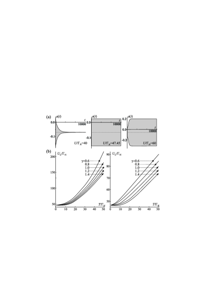
Figure 2: Characteristics of the mechanical dot vibrations as determined by Eqs. (2) and (29) for the NEM device sketched in Fig. 1: (a) Amplitude $a(t)$ of the dot vibrations (in units of the tunneling length $\lambda$) as a function of time $t$ (in units of $\hbar/\Gamma_{N}$, where $\Gamma_{N}=\Gamma_{L}\Gamma_{R}/(\Gamma_{L}+\Gamma_{R})$, $\Gamma_{L,R}$ are the widths of the energy level on the dot) for three different values of the Coulomb blockade energy $U$ at $T/{\Gamma_{N}}=5$. For small values of $U$ spontaneous vibrations are damped out (left panel), while for large $U$ they are amplified and develop into sustained finite-amplitude vibrations (right panel). A crossover between the two regimes occurs at $U=U_{c}$, when the vibration amplitude stays constant over time (middle panel). (b) Temperature dependence of the critical value of the Coulomb blockade energy $U_{c}(T)$ for a symmetric voltage biased device $\mu_{L}-\varepsilon_{F}=\varepsilon_{F}-\mu_{R}$ (left panel) and a device with a strongly biased drain electrode $\mu_{L}-\varepsilon_{F}\sim T,\varepsilon_{F}-\mu_{R}\gg T$ (right panel) for different values of the asymmetry parameter $\gamma=\Gamma_{R}/\Gamma_{L}$. The results were obtained for the following parameters: left lead bias $(\mu_{L}-\varepsilon_{F})=50\,\Gamma_{N}$, vibration frequency $\omega=1\,\Gamma_{N}/\hbar$, external magnetic field $H=0.5\,\Gamma_{N}/\mu_{B}$, magnetic exchange energy $J=1.5\,\Gamma_{N}$, dot level detuning energy $(\varepsilon_{0}-\varepsilon_{F})=2\,\Gamma_{N}$, and the electromechanical coupling constant $\kappa=\hbar^{2}J/(ml\lambda\Gamma_{N}^{2})=0.09$, where $\kappa$ is the coefficient multiplying r.h.s of Eq. (2) written in terms of dimensionless variables $x$ and $t$. For $\Gamma_{N}=$ 0.5 meV and $\lambda=l=$ 0.1 nm one finds that $m\sim 2\cdot 10^{-25}$ kg and $\omega\sim 2\pi\times 0.1$ THz are in reasonable agreement with experiments on single C₆₀ molecules trapped between metal electrodes mceuen ; park .

In order to analyze shuttle vibrations in the steady state, eventually reached after a shuttle instability, linearizing the problem with respect to dot displacements is not an adequate approach. Instead, one has to deal with the full nonlinear and nonlocal in time spintromechanical problem at hand numerically. In Fig. 2 we present results of numerical solutions to the coupled equations for the time-development of the density matrix components and of the mechanical oscillations of the dot, which are valid for arbitrary (not only small) dot displacements. In this case Eq. (2) has to be generalized by replacing the spintromechanical exchange force $\alpha=(2J/l)$ by a coordinate-dependent force, $\alpha\rightarrow(2J/l)\cosh\left(x(t)/l\right)$; $l$ is the decay length of the exchange interaction, and we consider a magnetically symmetric junction [SM, ].

Results of numerical simulations of the nonlinear and nonlocal temporal dynamics of the mechanical vibrations are presented in Fig. 2(a). One can readily see that, depending on how the Coulomb correlation energy $U$ is related to a critical value $U_{c}$, spontaneous small-amplitude vibrations are either damped out ($U<U_{c}$, left panel), maintained at a constant amplitude ($U=U_{c}$, middle panel) or amplified until they reach some steady-state amplitude $a_{0}$ ($U>U_{c}$, right panel).

It is remarkable that in the event of a shuttle instability [such as the one illustrated in the right panel of Fig. 2(a)] the mechanical vibration amplitude saturates even though no phenomenological friction term is included in Eq. (2). The physical explanation of this “self-saturation” effect is based on the fact that the electron shuttling phenomenon relies on retardation effects in the mechanical subsystem. These effects disappear in the limit of oscillation amplitudes that are large enough for the dot to come so close to the source and drain electrodes that the tunneling rate of charge relaxation becomes higher than the mechanical oscillation frequency.

In Fig. 2(b) (left panel) we present the numerically obtained temperature dependence of $U_{c}$ for different asymmetry parameters $\gamma$ and a symmetric biasing of the device, $\mu_{L}-\varepsilon_{F}=\varepsilon_{F}-\mu_{R}$. It is clearly seen from the figure that the linear temperature dependence of $U_{c}$, which is expected from the qualitative analysis, see Eqs. (5) and (1), holds rather accurately in the temperature range $25<T/\Gamma_{N}<45$. At higher temperatures the deviation from linearity becomes more pronounced due to a strong suppression of electron shuttling caused by electron parity fluctuations. An obvious reason for that is temperature stimulated population (ignored in Eq. (5)) of electronic states in the drain (right) electrode. This impedes electron tunneling to the drain lead thus suppressing the electric current through the device and diminishing the power supply to the mechanical vibrations. Such a blocking effect can be removed in asymmetrically biased device when $(\varepsilon_{F}-\mu_{R})/T\gg 1$, $(\mu_{L}-\varepsilon_{F})/T\sim 1$. The results of numerical simulations in this case are presented in Fig. 2(b), right panel. One can clearly see an accurate linear dependence in a large temperature interval in full agreement with Eq. (5). Moreover, using the value $n_{c}\simeq 0.28$ obtained in our numerical analysis, one finds from Eqs. (5) and (1) that the slope $s(n_{c},\gamma)\equiv dU_{c}/dT$ for $\gamma=1$ is $s(\gamma=1)\simeq 1.27$. This can be compared with the slope $s\simeq 1.0$ of the curve plotted for $\gamma=1$ in Fig. 2(b) (right panel). We conclude that there is good agreement between the exact numerical result and what we anticipated from our qualitative picture of Coulomb promoted magnetic-shuttle spintromechanics.

In conclusion, we have shown that Coulomb correlations play an important role for the nanomechanical properties of a magnetic shuttle device due to their ability to trigger a spintromechanical shuttle instability. Such an instability occurs when the Coulomb blockade charging energy exceeds a critical value, which depends on temperature and the strength of the enabling external magnetic field. The effect opens a possibility for single-electronic manipulation of spintromechanical performance.

Acknowledgement. This work was supported by the Institute for Basic Science in Korea (IBS-R024-D1); the Swedish Research Council (VR) ; the Croatian Science Foundation, project IP-2016-06-2289, and by the QuantiXLie Centre of Excellence, a project cofinanced by the Croatian Government and the European Union through the European Regional Development Fund - the Competitiveness and Cohesion Operational Programme (Grant KK.01.1.1.01.0004). The authors acknowledge the hospitality of PCS IBS in Daejeon (Korea).

Supplemental Material

The Hamiltonian of our spintromechanical system (see Fig. 1) consists of 3 terms

$$\hat{H}=\hat{H}_{l}+\hat{H}_{d}+\hat{H}_{t},$$ (6)

where $\hat{H}_{l}$ describes noninteracting spin-polarized electrons in the leads ( we assume that the leads are fully spin-polarized half-metals with anti-parallel magnetizations)

$$\hat{H}_{l}=\sum_{k,j}\varepsilon_{k,j}a_{k,j}^{\dagger}a_{k,j},\qquad j=L,R=\uparrow,\downarrow.$$ (7)

Here $a_{k,j}^{\dagger}$ $(a_{k,j})$ is the creation (annihilation) operator for an electron with momentum $k$ in lead $j$. We model the quantum dot by a single spin-degenerate electron level. The Hamiltonian of the quantum dot (QD) reads

$$\hat{H}_{d}=\sum_{\sigma}\varepsilon_{\sigma}c_{\sigma}^{\dagger}c_{\sigma}-h\left(c_{\uparrow}^{\dagger}c_{\downarrow}+c_{\downarrow}^{\dagger}c_{\uparrow}\right)+Uc_{\uparrow}^{\dagger}c_{\uparrow}c_{\downarrow}^{\dagger}c_{\downarrow}+\hat{H}_{m},$$ (8)

$$\hat{H}_{m}=\frac{p^{2}}{2m}+\frac{m\omega^{2}}{2}x^{2},$$ (9)

where $\varepsilon_{\sigma}=\varepsilon_{0}-(\sigma/2)J(x)$ is the spin- ($\sigma=\uparrow,\downarrow=+,-$) and position-dependent energy of the quantum dot spin-split levels ($\varepsilon_{0}$ is the level energy, $J(x)=J_{L}(x)-J_{R}(x)$ is the coordinate-dependent magnetic exchange energy per unit QD spin between the QD and the leads); $c_{\sigma}^{\dagger}$ $(c_{\sigma})$ is the creation (annihilation) operator for electron with spin projection $\sigma=\uparrow,\downarrow$ in the dot; $h\equiv g\mu_{B}H/2$ and $H$ is the external magnetic field, which is perpendicular to the plane of magnetization in the leads ($g$ is the gyromagnetic ratio, $\mu_{B}$ is the Bohr magneton), $U$ is the electron-electron repulsion energy. Vibrations of the dot are described by the Hamiltonian $H_{m}$ of a harmonic oscillator. In what follows we will treat $x$ and $p$ as classical variables.

In Eq.(6)-(8) and in the analysis below we neglect the voltage-dependent electric force on the dot in comparison with the magnetic exchange force. This is a good approximation if the electric field ${\cal E}$ acting on the shuttle is sufficiently weak. If ${\cal E}$ is increased there is at some point a transition from the regime of spintromechanical shuttling discussed here to electromechanical shuttling for which the parity effect is obviously irrelevant. A description of this transition is beyond the scope of the present paper.

The tunneling of electrons between lead $j=L,R=-,+$ and a movable QD is described by a tunneling Hamiltonian with coordinate-dependent tunneling amplitude $t_{j}(x)=t_{j}\exp(jx/\lambda)$, $\lambda$ is the characteristic tunneling length,

$$\hat{H}_{t}=t_{L}(x)\sum_{k}c^{\dagger}_{\uparrow}a_{k,L}+t_{R}(x)\sum_{k}c^{\dagger}_{\downarrow}a_{k,R}+\text{h.c.}$$ (10)

We solve the problem of mechanical instability in our NEM system by using the density operator method. The density operator obeys the von Neumann equation $(\hbar=1)$

$$i\partial_{t}\hat{\rho}(t)=[\hat{H},\hat{\rho}(t)].$$ (11)

In what follows we consider the regime of sequential electron tunneling in the NEM transistor ($\text{max}\{T,\mu_{L}-\mu_{R}\}\gg\Gamma$, where $\Gamma$ is the width of the electron energy level in the dot, $T$ is the temperature, $\mu_{L}$, $\mu_{R}$ are the chemical potentials in the leads). Then the total density operator is factorized, $\hat{\rho}(t)\approx\hat{\rho}_{d}(t)\otimes\hat{\rho}_{l}$, where $\hat{\rho}_{d}(t)$ is the QD density operator and $\hat{\rho}_{l}$ is the equilibrium density matrix of the leads. By tracing out the leads’ degrees of freedom it is straightforward to derive a set of equations for the matrix elements of $\hat{\rho}_{d}$ in the Fock space of a single level QD: $\rho_{0}=\langle 0|\hat{\rho}_{d}|0\rangle$, $\rho_{\uparrow}=\langle\uparrow|\hat{\rho}_{d}|\uparrow\rangle$, $\rho_{\downarrow}=\langle\downarrow|\hat{\rho}_{d}|\downarrow\rangle$, $\rho_{\uparrow\downarrow}=\langle\uparrow|\hat{\rho}_{d}|\downarrow\rangle=\rho_{\downarrow\uparrow}^{\ast}$, $\rho_{2}=\langle 2|\hat{\rho}_{d}|2\rangle$. One finds that

$$|\dot{\rho}_{j}\rangle=\hat{A}_{\rho}|\rho_{j}\rangle,$$ (12)

where the $6\times 6$ matrix $\hat{A}_{\rho}$ has the form

$$\hat{A}_{\rho}=\left(\begin{array}[]{cccccc}A_{11}&A_{12}&A_{13}&A_{14}&A_{14}^{\ast}&0\\ A_{21}&A_{22}&0&A_{24}&A_{24}^{\ast}&A_{26}\\ A_{31}&0&A_{33}&A_{34}&A_{34}^{\ast}&A_{36}\\ A_{41}&A_{42}&A_{43}&A_{44}&0&A_{46}\\ A_{41}^{\ast}&A_{42}^{\ast}&A_{43}^{\ast}&0&A_{44}^{\ast}&A_{46}^{\ast}\\ 0&A_{62}&A_{63}&A_{64}&A_{64}^{\ast}&A_{66}\\ \end{array}\right),$$ (13)

with the following matrix elements $A_{ij}$:

$$A_{11} = -\Gamma_{L}(x)f_{L}^{+}-\Gamma_{R}(x)f_{R}^{+}-\Upsilon_{1L}(x)+\Upsilon_{1R}(x),\;A_{12}=\Gamma_{L}(x)(1-f_{L}^{+})-\Upsilon_{1L}(x),$$ (14)

$$A_{13} = \Gamma_{R}(x)(1-f_{R}^{+})+\Upsilon_{1R}(x),\;A_{14}=-\Upsilon_{2L}(x)-\Upsilon_{2R}(x),$$ (15)

$$A_{21} = \Gamma_{L}(x)f_{L}^{+}+\Upsilon_{1L}(x),\;A_{22}=-\Gamma_{L}(x)(1-f_{L}^{+})-\Gamma_{R}(x)f_{R}^{U,+}+\Upsilon_{1L}(x)+\Upsilon_{1R}^{U}(x),$$ (16)

$$A_{24} = -ih+\Upsilon_{2L}(x)+\Upsilon_{2R}^{U}(x),\;A_{26}=\Gamma_{R}(x)(1-f_{R}^{U,+})+\Upsilon_{1R}^{U}(x),$$ (17)

$$A_{31} = \Gamma_{R}(x)f_{R}^{+}-\Upsilon_{1R}(x),\;A_{33}=-\Gamma_{R}(x)(1-f_{R}^{+})-\Gamma_{L}(x)f_{L}^{U,+}-\Upsilon_{1L}^{U}(x)-\Upsilon_{1R}(x),$$ (18)

$$A_{34} = ih+\Upsilon_{2R}(x)+\Upsilon_{2L}^{U}(x),\;A_{36}=\Gamma_{L}(x)(1-f_{L}^{U,+})-\Upsilon_{1L}^{U}(x),$$ (19)

$$A_{41} = \Upsilon_{2L}(x)+\Upsilon_{2R}(x),\;A_{42}=-ih+\Upsilon_{2L}(x)+\Upsilon_{2R}^{U}(x),\;A_{43}=ih+\Upsilon_{2R}(x)+\Upsilon_{2L}^{U}(x),$$ (20)

$$A_{44} = iJ(x)-\frac{1}{2}\Gamma_{L}(x)(1-f_{L}^{+}+f_{L}^{U,+})-\frac{1}{2}\Gamma_{R}(x)(1-f_{R}^{+}+f_{R}^{U,+})$$ (21)

$$- \frac{1}{2}\left[\Upsilon_{1L}(x)-\Upsilon_{1L}^{U}(x)-\Upsilon_{1R}(x)+\Upsilon_{1R}^{U}(x)\right],$$

$$A_{46} = \Upsilon_{2L}^{U}(x)+\Upsilon_{2R}^{U}(x),\;A_{62}=\Gamma_{R}(x)f_{R}^{U,+}-\Upsilon_{1R}^{U}(x),\;A_{63}=\Gamma_{L}(x)f_{L}^{U,+}+\Upsilon_{1L}^{U}(x),$$ (22)

$$A_{64} = -\left[\Upsilon_{2L}^{U}(x)+\Upsilon_{2R}^{U}(x)\right],\;A_{66}=-\Gamma_{L}(x)(1-f_{L}^{U,+})-\Gamma_{R}(x)(1-f_{R}^{U,+})+\Upsilon_{1L}^{U}(x)-\Upsilon_{1R}^{U}(x).$$ (23)

In Eqs. (14)–(23) we introduced the following notations,

$$\Upsilon_{1L/R}(x) = f_{L/R}^{-}\frac{J(x)\Gamma_{L/R}(x)}{\sqrt{J^{2}(x)+4h^{2}}},\;\Upsilon_{1L/R}^{U}(x)=f_{L/R}^{U,-}\frac{J(x)\Gamma_{L/R}(x)}{\sqrt{J^{2}(x)+4h^{2}}},$$ (24)

$$\Upsilon_{2L/R}(x) = f_{L/R}^{-}\frac{h\Gamma_{L/R}(x)}{\sqrt{J^{2}(x)+4h^{2}}},\;\Upsilon_{2L/R}^{U}(x)=f_{L/R}^{U,-}\frac{h\Gamma_{L/R}(x)}{\sqrt{J^{2}(x)+4h^{2}}};$$ (25)

here

$$2f_{L,R}^{\pm} = f_{L,R}(E_{-})\pm f_{L,R}(E_{+}),\;2f_{L,R}^{U,\pm}=f_{L,R}(E_{-}+U)\pm f_{L,R}(E_{+}+U),$$ (26)

and

$$E_{\pm}=\varepsilon_{0}\pm\frac{\sqrt{J^{2}(x)+4h^{2}}}{2},$$ (27)

$$f_{j}(\epsilon)=\left\{1+\exp[(\epsilon-\mu_{j})/T_{j}]\right\}^{-1}.$$ (28)

We use the system of equations (12) for numerical calculations (see main text).

For analytical calculations it is convenient to use linear combinations of $\rho_{j}$. Then the symmetric spin-neutral combination $R_{0}=\rho_{0}+\rho_{2}$ (and $\rho_{\uparrow}+\rho_{\downarrow}=1-\rho_{0}-\rho_{2}$) is decoupled from the other four quantities $R_{1}=\rho_{0}-\rho_{2}$, $R_{2}=\rho_{\uparrow}-\rho_{\downarrow}$, $R_{3}=-i(\rho_{\uparrow\downarrow}-\rho_{\uparrow\downarrow}^{\ast})$, $R_{4}=\rho_{\uparrow\downarrow}+\rho_{\uparrow\downarrow}^{\ast}$. The system of equations for $R_{j}$ $(j=1-4)$ takes the form

$$|\dot{R}(t)\rangle=\hat{A}\{x(t),U\}|R(t)\rangle+|B\{x(t),U\}\rangle,$$ (29)

with $\hat{A}\{x(t),U\}=\hat{A}_{\Gamma}\{x(t),U\}+\hat{A}_{H}\{x(t),U\}+\hat{A}_{J}\{x(t),U\}$. Here we introduced matrices related to tunneling (subindex $\Gamma$), the external magnetic field (subindex $H$) and the exchange interaction (subindex $J$)

$$\hat{A}_{\Gamma}\{x(t),U\}=-\frac{1}{2}\left(\begin{array}[]{cccc}F_{+}^{+,-}(x,U)&-F_{-}^{-,+}(x,U)&0&0\\ -F_{-}^{+,-}(x,U)&F_{+}^{-,+}(x,U)&0&0\\ 0&0&F_{+}^{-,+}(x,U)&0\\ 0&0&0&F_{+}^{-,+}(x,U)\\ \end{array}\right),$$ (30)

$$\hat{A}_{H}\{x(t),U\}=\left(\begin{array}[]{cccc}0&0&0&-H_{+}^{-}(x,U)\\ 0&0&2h&H_{-}^{-}(x,U)\\ 0&-2h&0&0\\ H_{+}^{-}(x,U)&H_{-}^{-}(x,U)&0&0\\ \end{array}\right),$$ (31)

$$\hat{A}_{J}\{x(t),U\}=\frac{1}{2}\left(\begin{array}[]{cccc}-J_{-}^{-}(x,U)&-J_{+}^{-}(x,U)&0&0\\ J_{+}^{-}(x,U)&J_{-}^{-}(x,U)&0&0\\ 0&0&-J_{-}^{-}(x,U)&J(x)\\ 0&0&-J(x)&J_{-}^{-}(x,U)\\ \end{array}\right),$$ (32)

$$|B\{x(t),U\}\rangle=\frac{1}{2}\left(\begin{array}[]{c}F_{+}^{-,-}(x,U)-J_{-}^{+}(x,U)\\ -F_{-}^{-,-}(x,U)+J_{+}^{+}(x,U)\\ 0\\ 2H_{+}^{+}(x,U)\\ \end{array}\right).$$ (33)

Here we denote

$$F_{\pm}^{j,k}(x,U)=\Gamma_{\pm}(x)+j\left[\Gamma_{L}(x)f_{L}^{+}\pm\Gamma_{R}(x)f_{R}^{+}\right]+k\left[\Gamma_{L}(x)f_{L}^{U,+}\pm\Gamma_{R}(x)f_{R}^{U,+}\right],$$ (34)

with $j,k=(+,-)$

$$H_{\pm}^{\eta}(x,U)=\left\{\Gamma_{L}(x)f_{L}^{-}\pm\Gamma_{R}(x)f_{R}^{-}+\eta\left[\Gamma_{L}(x)f_{L}^{U,-}\pm\Gamma_{R}(x)f_{R}^{U,-}\right]\right\}\frac{h}{\sqrt{4h^{2}+J^{2}(x)}},$$ (35)

$$J_{\pm}^{\eta}(x,U)=\left\{\Gamma_{L}(x)f_{L}^{-}\pm\Gamma_{R}(x)f_{R}^{-}+\eta\left[\Gamma_{L}(x)f_{L}^{U,-}\pm\Gamma_{R}(x)f_{R}^{U,-}\right]\right\}\frac{J(x)}{\sqrt{4h^{2}+J^{2}(x)}};$$ (36)

and $\eta=\pm 1$. Notice that $H_{\pm}^{\eta}(x,U)/h=J_{\pm}^{\eta}(x,U)/J(x)$. In Eq. (34) the notation $\Gamma_{\pm}(x)=\Gamma_{L}(x)\pm\Gamma_{R}(x)$ is introduced.

In the case of non-interacting electrons, $U=0$, the analytic solution can be simplified for a symmetric tunnel junction, $\Gamma_{L}(x=0)=\Gamma_{R}(x=0)=\Gamma$, $J_{L}(x=0)=J_{R}(x=0)$. We solve the system (29) by perturbation theory with $R_{i}(t)\approx R_{i}^{0}+R_{i}^{1}(t)$, $R_{i}^{1}(t)\propto x(t)$, assuming the displacement $x$ to be small. Then the equations for $R_{1}^{1}$ and $R_{4}^{1}$ are decoupled from the equations for $R_{2}^{1}$ and $R_{3}^{1}$. Therefore the analysis of the mechanical instability in this particular case is reduced to a simpler problem — one has to solve two coupled linear equations

$$\left(\begin{array}[]{c}\dot{R}_{2}^{1}\\ \dot{R}_{3}^{1}\end{array}\right)=\left(\begin{array}[]{cc}-\Gamma&2h\\ -2h&-\Gamma\end{array}\right)\left(\begin{array}[]{c}R_{2}^{1}\\ R_{3}^{1}\end{array}\right)-\alpha(f_{L}^{-}+f_{R}^{-})\left(\begin{array}[]{c}\Gamma/(2h)\\ 1\end{array}\right)x(t),$$ (37)

where $\alpha>0$ (the exchange force per unit QD spin) is the derivative of the exchange energy per unit QD spin, $J(x)\approx-\alpha x$ (Cf. Fig. 1). Substituting the solution $R_{2}^{1}$ into Eq. (2) of the main text, we obtain the desired Eq. (6).

References

(1)Single Charge Tunneling (H. Grabert, M.H. Devoret, Eds.),
Plenum, New York (1992).
(2)
I. Zutic, J. Fabian, S. Das Sarma, Rev. Mod. Phys.76,
323 (2004).
(3)
R.I. Shekhter, A. Pulkin, M. Jonson, Phys. Rev. B86,
100404(R) (2012).
(4)
M. Poot, H.S.J. van der Zant, Phys. Rep.511, 273
(2012).
(5)
Abhay N. Pasupathy, Radoslaw C. Bialczak, Jan Martinek, Jacob E. Grose,
Luke A. K. Donev, Paul L. McEuen, and Daniel C. Ralph Science306, 86
(2004).
(6) M.P. Blencowe, Contemp. Phys.
46, 249 (2005).
(7) J.S. Aldridge, A.N. Cleland,
R. Knobel, D.R. Schmidt, C.S. Yung, Proceedings of Spie — the
International Society for Optical Engineering 4591, 11
(2001).
(8) A. Erbe, C. Weiss, W. Zwerger,
R.H. Blick, Phys. Rev. Lett. 87(9), 096106 (2001).
(9) F. Pistolesi, Phys. Rev. B 69(24), 245409 (2004).
(10)
S.I. Kulinich, L.Y. Gorelik, A.N. Kalinenko, I.V. Krive,
R.I. Shekhter, Y.W. Park, and M. Jonson, Phys. Rev. Lett.112, 117206 (2014).
(11)
O.A. Ilinskaya, S.I. Kulinich, I.V. Krive, R.I. Shekhter,
H.C. Park, and M. Jonson, New J. Phys.20, 063036
(2018).
(12)
See Supplemental Material at [URL will be inserted by publisher] for details.
(13)
Hongkun Park, Jiwoong Park, Andrew K. L. Lim, Erik H. Anderson, A. Paul Alivisatos, and Paul L. McEuen,
Nature 407, 58 (2000).