Does spatial flatness forbid the turnaround epoch of collapsing structures?

Abstract

Cosmological observational analysis frequently assumes that the Universe is spatially flat. We aim to non-perturbatively check the conditions under which a flat or nearly flat expanding dust universe, including the $\Lambda$-cold-dark-matter ($\Lambda$CDM) model if interpreted as strictly flat, forbids the gravitational collapse of structure. We quantify spatial curvature at turnaround. We use the Hamiltonian constraint to determine the pointwise conditions required for an overdensity to reach its turnaround epoch in an exactly flat spatial domain. We illustrate this with a plane-symmetric, exact, cosmological solution of the Einstein equation, extending earlier work. More generally, for a standard initial power spectrum, we use the relativistic Zel’dovich approximation implemented in inhomog to numerically estimate how much positive spatial curvature is required to allow turnaround at typical epochs/length scales in almost-Einstein–de Sitter (EdS)/$\Lambda$CDM models with inhomogeneous curvature. We find that gravitational collapse in a spatially exactly flat, irrotational, expanding, dust universe is relativistically forbidden pointwise. In the spatially flat plane-symmetric model considered here, pancake collapse is excluded both pointwise and in averaged domains. In an almost-EdS/$\Lambda$CDM model, the per-domain average curvature in collapsing domains almost always becomes strongly positive prior to turnaround, with the expansion-normalised curvature functional reaching $\Omega_{{\cal R}}^{{\cal D}}\sim-5$. We show analytically that a special case gives $\Omega_{{\cal R}}^{{\cal D}}=-5$ exactly (if normalised using the EdS expansion rate) at turnaround. An interpretation of $\Lambda$CDM as literally 3-Ricci flat would forbid structure formation. The difference between relativistic cosmology and a strictly flat $\Lambda$CDM model is fundamental in principle, but we find that the geometrical effect is weak.

1 Introduction

We investigate the degree to which the spatial flatness of a compact spatial domain of the Universe would relativistically prevent the domain from gravitationally collapsing. Cosmological observations are usually analysed by modelling the Universe as a Friedmann–Lemaître–Robertson–Walker (FLRW) [1, 2, 3] model with a flat comoving spatial section (e.g. [4, 5, 6, 7]; and [8] apart from the gravitational lensing analyses therein; and references therein). However, this use of flatness for calculations coexists with the contradictory characteristic of spatially inhomogeneous curvature. The seeds of structure formation are frequently modelled as early epoch curvature pertubations associated with density pertubations, in linear perturbation theory [e.g. 9, and references therein], and allowed to grow into non-linear gravitationally collapsed (or nearly emptied) structures by the current epoch, based on the hypothesis that the perturbed solutions are good approximations to exact solutions of the Einstein equation for as long as the perturbations remain weak. Empirically, this mathematical hypothesis seems to be a posteriori reasonable. However, the Einstein equation imposes constraints that are still being explored and not yet completely understood. Non-perturbative, exact, nearly-FLRW cosmological solutions of the Einstein equation [for a review, see 10] can, as we show here, provide stronger constraints on structure formation than those provided by linear perturbation theory. It is important to improve our understanding of the distinction between the $\Lambda$CDM ($\Lambda$ cold dark matter) model, interpreted literally as having flat FLRW spatial sections with non-linear curvature inhomogeneities that by coincidence cancel exactly to a uniform, flat average background, versus strictly general-relativistic models that account for structure formation with as few linearisations as possible. Better understanding of inhomogeneous curvature at the scale of a few tens of megaparsecs can potentially contribute to the understanding of large-scale average scalar curvature. This is especially important in the context of the upcoming generation of major extragalactic surveys including those of ground-based photometric projects such as LSST (Large Synoptic Survey Telescope; [11]), spectroscopic projects such as 4MOST (4-metre Multi-Object Spectroscopic Telescope; [12, 13]), DESI (Dark Energy Spectroscopic Instrument; [14]) and eBOSS (extended Baryon Oscillation Spectroscopic Survey; [15]), and the space-based projects Euclid [16] and COREmfive [17, 18, 19].

As a step towards this clarification, the primary aim of this work is to non-perturbatively check the conditions under which a flat or nearly flat expanding dust (general-relativistic) universe forbids the gravitational collapse of structure. By ‘flat’, we refer to the spatial curvature for a flow-orthogonal spacetime foliation, as detailed below in Sect. 2.1. This foliation is defined by a physical criterion and is thus gauge independent (see Sect. 4.1 for more discussion).

While Newtonian gravity in standard $N$-body simulations can be interpreted as requiring positive spatial curvature for gravitational collapse, this relativistic interpretation only follows from a quite restricted line of reasoning. This ‘Newtonian limit’ argument follows from a Newtonian slicing (a Newtonian-gauge restriction) of a relativistic cosmological spacetime with a spatial section that is topologically $\mathbb{E}^{3}$ or $\mathbb{S}^{1}\times\mathbb{S}^{1}\times\mathbb{S}^{1}$ and that has a line element restricted to

$$\mathrm{d}s^{2} =a^{2}\left\{-(1+2\psi)\,\mathrm{d}\tau^{2}+(1-2\varphi)\left[\mathrm{d}x^{2}+\mathrm{d}y^{2}+\mathrm{d}z^{2}\right]\right\}\,,$$ (1.1)

where $a=a(\tau)$ is a flat FLRW background scale factor depending on conformal time $\tau$, and $\psi$ and $\varphi$ are scalar fields on the spacetime. The 3-Ricci scalar curvature is

$${}^{3}R={{8\,\varphi\,\left(\varphi_{,x\,x}+\,\varphi_{,y\,y}+\,\varphi_{,z\,z}\right)-4\,\left(\varphi_{,x\,x}+\,\varphi_{,y\,y}+\,\varphi_{,z\,z}\right)-6\,\left(\varphi_{,x}^{2}+\,\varphi_{,y}^{2}+\,\varphi_{,z}^{2}\right)}\over{a^{2}\,\left(2\,\varphi-1\right)^{3}}}\,,$$ (1.2)

where commas indicate partial derivatives. For linear perturbation theory with a slowly varying potential $\varphi$ and weak second derivatives of the potential, that is, for $|\varphi|\ll 1,\;|\varphi_{,x^{i}}|\ll 1,\;|\varphi_{,x^{i}x^{i}}|\ll 1\;\forall x^{i}\in\{x,y,z\}$, Eq.  (1.2) can be approximated as

$${}^{3}R \approx 4\,a^{-2}\,\left(\varphi_{,x\,x}+\varphi_{,y\,y}+\varphi_{,z\,z}\right)$$

$$=4\,a^{-2}\,\nabla_{\mathbb{E}^{3}}^{2}\varphi$$

$$=16\pi\,G\,\delta\rho\,,$$ (1.3)

for an overdensity $\delta\rho$, where the final line follows from the Newtonian expanding universe form of Poisson’s equation. Thus, since gravitational collapse will usually require a positive overdensity, this should be associated with positive spatial curvature in the Newtonian restriction if the potential $\varphi$ and its first and second derivatives are weak enough. (For wider discussion, see especially Eq. (4.5) of [20]; or [9] and references therein.) Here, we do not make these restrictions.

Beyond this interpretive, approximate, Newtonian-gauge–restriction sense, the Newtonian formulae and vector space structure of standard $N$-body simulations are not modified to take into account spatial curvature. Thus, the ‘Newtonian cosmology’ that directly enters into calculations that are coded in the non-linear evolution of standard $N$-body simulations [e.g. 21, 22, 23, 24], is, in principle, relativistically inaccurate by not taking into account curvature beyond this intepretive sense. Here, by Newtonian cosmology we mean work such as that of [25] and the terminology of Ellis ([26]; [27], p. 611), who observes that spatial curvature is ‘essentially general-relativistic in character’ and that the 3-Ricci tensor ‘has no Newtonian analogue’, and of Ellis et al. [28, p. 149], who note that in Newtonian cosmology, the Friedmann equation curvature constant is ‘a constant of integration, with no relation to spatial curvature’.

In standard $N$-body simulations, spatial flatness is built into the simulations via two-point flat-space Newtonian gravitational attraction for the ‘particle-particle’ mode of calculation, Fourier analysis for the ‘mesh’ mode of calculating gravitational potentials, vector arithmetic (in the universal covering space) that is undefined in a space that is not a vector space, and distance calculations that use a flat FLRW metric (not an inhomogeneous Newtonian-gauge metric). Using these methods is consistent with the assumptions of Newtonian cosmology (in the sense defined above), reliant on the notion of an absolute spacetime, which provides a flat embedding for cosmological fluid trajectories. In Newtonian cosmology, one can change from Eulerian coordinates, associated with the absolute spacetime, to Lagrangian coordinates, which trace fluid evolution. This allows associating the relativistic notions of extrinsic and intrinsic spatial curvature to properties of fluid trajectories in Newtonian cosmology. The fact that the Eulerian to Lagrangian coordinate transformation is invertible prior to shell crossing sometimes leads to the belief that the extrinsic and intrinsic curvatures are merely artefacts of a specific coordinate system. In particular, in the context of cosmological perturbation theory, a diffeomorphism is used to map between the curved manifold and a flat background with pulled-back fields, giving the misleading impression that scalar quantities associated with curvature are not invariant.

To the best of our knowledge, it has not been shown prior to this work that positive intrinsic spatial curvature in the fluid rest frame is unavoidable if a collapsing domain is to reach the turnaround epoch, apart from the approximate, Newtonian-gauge–restriction argument above that imposes several restrictive assumptions. This is yet another example of how extrinsic and intrinsic curvatures are real physical quantities that are not removable by any coordinate transformation.

With the aim of developing new tests for observational cosmology, we also wish to estimate approximate values of positive spatial curvature that are required at characteristic mass scales and epochs in the almost-Einstein–de Sitter (EdS) and almost-$\Lambda$CDM models in order to allow overdensities to reach their turnaround epochs. We use the term ‘almost-’ to indicate that inhomogeneous spatial curvature is allowed in the models. The initial spatial curvature at any point or region is typically weak. However, in contrast to the evolution of the spatially constant curvature of a non-flat FLRW model, which is static in FLRW comoving units but weakens in physical inverse square length units as the Universe expands, generic spatial curvature evolution tends to strengthen initially weak curvature.

Moreover, we show that the positive curvature at turnaround must, at least in a particular EdS case, occur at a particular critical value. The motivation for considering the EdS case is that a cosmic microwave background (CMB) normalised EdS model together with structure formation may provide the extra 16% expansion (scale factor value) needed for the combined model to be observationally viable without dark energy [29, Eq. (13)].

Following the standard FLRW and scalar averaging conventions, the expansion-rate–normalised curvature functional adopted here ($\Omega_{{\cal R}}^{{\cal D}}$, see Eq. (2.7)) has the opposite sign to that of the scalar curvature itself. In the scalar averaging context, the ‘Omegas’ are referred to as functionals rather than parameters, because they depend on fields on spatial hypersurfaces. We set the initial values of the average scale factor in a domain ${\cal D}$, of the effective (globally averaged) scale factor, and of $a(t)$, to be equal, that is, we set $a_{{\cal D}}({{t}_{\mathbf{i}}})$ and $a_{\mathrm{eff}}({{t}_{\mathbf{i}}})$ to be equal to $a({{t}_{\mathbf{i}}})$, respectively, where this value is normalised to the CMB value using a $\Lambda$CDM proxy that reaches a unity scale factor at the current epoch, as detailed in Sect. 2.4.2.

In Sect. 2 we present our method, including definitions and terminology in Sect. 2.1, the Hamiltonian constraint in Sect. 2.2, and the definition of an illustrative, one–free-function, plane-symmetric case in Sect. 2.3. In Sect. 2.4 we describe how we analytically investigate a special case of initial conditions in an almost-EdS model (Sect. 2.4.1), and in the more general case, for standard cosmological $N$-body simulation initial conditions, for the EdS and $\Lambda$CDM cases (Sect. 2.4.2), where we also include the effects of scalar averaging. Results are given in Sect. 3. In Sect. 3.1 we examine the pointwise (unaveraged) Hamiltonian constraint, which relates, in particular, the expansion rate, density and curvature. In Sect. 3.2 we consider the plane-symmetric, exact, flat, expanding universe example. In Sect. 3.3 we present the results in a special analytical almost-EdS case that yields a critical value (Sect. 3.3.1) and more general numerical results in the almost-EdS and almost-$\Lambda$CDM cases (Sect. 3.3.2). We discuss the results in Sect. 4 and applications to numerical general relativity in Sect. 4.4, and conclude in Sect. 5.

2 Method

2.1 Universe model

As in [30] and following [31, 32], we generalise beyond the FLRW model, allowing initial inhomogeneities to, a priori, gravitationally collapse, expand and become voids, or form more complex structures that together yield the cosmic web, as follows. We adopt the notation of [33] for an irrotational dust universe foliated by flow-orthogonal spatial sections that are labelled by a time coordinate $t$ defined by the fluid proper time. This notation differs slightly from that of [30]. We adopt Roman indices to indicate spatial coordinates, we use the Einstein summation convention, and an overdot ($\dot{\ }$) indicates derivatives with respect to $t$. An FLRW ‘reference model’ (not necessarily an average model; we thus avoid the ambiguous term ‘background model’) is used here, with scale factor $a(t)$. The extrinsic curvature $K^{i}_{j}$ is used to define the expansion tensor $\Theta^{i}_{j}:=-K^{i}_{j}$, the expansion scalar (without removal of a reference model Hubble–Lemaître flow; [34, 2, 35]) $\Theta:=\Theta^{i}_{i}\equiv-K^{i}_{i}$, and the peculiar-expansion tensor $\theta^{i}_{j}:=\Theta^{i}_{j}-H\,\delta^{i}_{j}$ (for the Kronecker delta $\delta^{i}_{j}$), where a reference model expansion rate $H:=\dot{a}/a$ is subtracted; the shear tensor is defined $\sigma^{i}_{j}:=\Theta^{i}_{j}-\frac{1}{3}\Theta\,\delta^{i}_{j}$ and the shear scalar $\sigma^{2}:=\frac{1}{2}\sigma^{i}_{j}\,\sigma^{j}_{i}$; the spatial scalar curvature is ${\cal R}:={\cal R}^{i}_{i}$; density is $\rho$; the gravitational constant is $G$; and an optional cosmological constant is $\Lambda$.

The FLRW models solve the Einstein equation in a way in which $a^{2}(t)\,{\cal R}$ is spatially constant (curvature is set to be homogeneous) and setting $\theta^{i}_{j}=0$, or equivalently, $\sigma^{i}_{j}=0$ and $\Theta=3H$. The EdS and $\Lambda$CDM models are part of the FLRW subcase in which ${\cal R}=0$. In sections Sections 2.4 and 3.3 we consider models that are almost-FLRW at early times.

2.2 Hamiltonian constraint

The time–time component of the Einstein equation gives the Hamiltonian constraint [36, 37, 38, 39], which is presented in an elegant form in [30, Eq. (4a)]:

$$\frac{1}{3}\Theta^{2} =8\pi G\rho+\sigma^{2}-\frac{1}{2}{\cal R}+\Lambda\,.$$ (2.1)

In Sect. 3.1, we use this equation to determine the conditions required for an initially weak overdensity expanding with the rest of the Universe to decelerate and reach its turnaround epoch at points that are exactly flat spatially. The above equation generalises the Friedmann equation of the FLRW model, which can be written with terms matching, respectively, those of Eq. (2.1),

$$3\,H^{2} =3\,H^{2}\Omega_{\mathrm{m}}+0+3\,H^{2}\Omega_{\mathrm{k}}+3\,H^{2}\Omega_{\Lambda}\,,$$ (2.2)

with matter density parameter $\Omega_{\mathrm{m}}$, curvature parameter $\Omega_{\mathrm{k}}$, and dark energy parameter $\Omega_{\Lambda}$, all of which are given here as time-dependent values, not current-epoch constants.

2.3 Plane-symmetric subcase

We illustrate the blocking of gravitational collapse (inability to reach the turnaround epoch) with an exact non-perturbative solution of the Einstein equation. This is a subcase of the plane-symmetric case, which has been considered by several authors ([40, 41, 42]; [43]). The existence of this exact but reasonably simple inhomogeneous cosmology solution (a Szekeres model; [44]) potentially offers a powerful method of calibrating relativistic cosmology software. Here, we examine the subcase in the form that has an ‘exact perturbation’ $P(w,t)$ in a single direction $w$ in a universe whose spatial section is either the infinite Euclidean space $\mathbb{E}^{3}$ or the 3-torus $\mathbb{T}^{3}$. By ‘exact perturbation’, we mean that the perturbation $P$ can be studied without Taylor expansions in $P$ and without dropping any Taylor or non-Taylor high-order terms in $P$.

The metric is expressed here as [33, Eq. (66), Sect. V.A],

$$\mathrm{d}s^{2}= -\mathrm{d}t^{2}+a(t)^{2}\left[\mathrm{d}x^{2}+\mathrm{d}y^{2}+\left(1+P(w,t)\rule{0.0pt}{8.61108pt}\right)^{2}\mathrm{d}w^{2}\right],$$ (2.3)

with flow-orthogonal spatial sections, where $P$ is by definition a plane-symmetric function, which we require to be smooth. Inserting this metric into the Einstein equation shows that the scale factor $a(t)$ and the associated expansion rate $H(t):=\dot{a}/a$ must be the standard flat FLRW solutions (for arbitrary $\Lambda$). In other words, $a(t)$ has to be the scale factor solution for what we can consider to be a flat ‘reference model’ universe. The coordinates $x,y,w$ are comoving with the fluid. We assume as an initial condition at an early epoch that $|P(w,{{t}_{\mathbf{i}}})|\ll 1$. Situations in which the line element in the inhomogeneous direction $w$ is compressed to zero, that is, in which $\lim_{t\rightarrow t_{\mathrm{coll}}^{+}}P=-1$ at an epoch $t_{\mathrm{coll}}$, can be expected to represent gravitational ‘pancake’ collapse. In Sect. 3.2, we consider whether an initial overdensity defined on a $w$ plane of the function $P$ can decelerate sufficiently to reach its turnaround epoch, and extend the EdS reference model case considered by [33] to also include the case of a $\Lambda$CDM reference model.

To extend this analysis from pointwise collapse to averaged collapse within a comoving spatial domain ${\cal D}$ using the spatial metric volume element $\mathrm{d}\mu_{\mathbf{g}}$, we need the scalar averaging operator $\left\langle.\right\rangle_{\cal D}$, defined for a scalar field ${\cal A}$ as

$$\left\langle{\cal A}\right\rangle_{\cal D}:=\frac{\int_{{\cal D}}{\cal A}\,\mathrm{d}\mu_{\mathbf{g}}}{\int_{{\cal D}}\mathrm{d}\mu_{\mathbf{g}}}$$ (2.4)

(see also Eq. (2.12) below). Applying this to Eq. (2.1) and shifting $\left\langle\Theta^{2}\right\rangle_{\cal D}/3$ to the right-hand side yields

$$\frac{1}{3}\left\langle\Theta\right\rangle_{\cal D}^{2} =8\pi G\left\langle\rho\right\rangle_{\cal D}+\left\langle\sigma^{2}\right\rangle_{\cal D}-\frac{1}{3}\left\langle\left(\Theta-\left\langle\Theta\right\rangle_{\cal D}\right)^{2}\right\rangle_{\cal D}-\frac{1}{2}\left\langle{\cal R}\right\rangle_{\cal D}+\Lambda$$ (2.5)

[33, Eqs (10), (11), and references therein].

2.4 Almost-Einstein–de Sitter and almost-$\Lambda$CDM models

Since a realistic cosmological model must allow gravitational collapse of density perturbations, the results below (Sect. 3.1, Sect. 3.2) imply that positive spatial curvature has to be allowed in such a model in order to allow pointwise turnaround to be reached. The scalar-averaged behaviour in a spatial domain, as represented in Eq. (2.5), has an extra term in the right-hand side. Since $\left\langle\left(\Theta-\left\langle\Theta\right\rangle_{\cal D}\right)^{2}\right\rangle_{\cal D}$ is necessarily non-negative, it could, in principle, provide an alternative physical driver than positive curvature for allowing gravitational collapse through to the turnaround epoch, provided that it is sufficiently bigger than the averaged shear scalar $\left\langle\sigma^{2}\right\rangle_{\cal D}$. To study this, as shown in [45], [46], and [33, and references therein] and implemented with free-licensed software as shown in [47], the relativistic Zel’dovich approximation (RZA) can be used to model gravitational collapse and void formation in the cosmological context much faster than using $N$-body simulations, without any need to assume spherically symmetric collapse, and permitting positive (and non-positive) spatial scalar curvature. This is done by integrating the averaged Raychaudhuri equation, where the averaging corresponds to a Lagrangian spatial domain ${\cal D}$, starting with standard cosmological inhomogeneous initial conditions. This equation yields $\ddot{a}_{{\cal D}}$, the second time derivative of the per-domain average scale factor $a_{{\cal D}}$, and depends, in particular, on the temporal evolution of the kinematical backreaction functional. The kinematical backreaction functional, defined [33, Eq. (11)]

$${\cal Q}_{{\cal D}} :=\frac{2}{3}\left\langle\left(\Theta-\left\langle\Theta\right\rangle_{\cal D}\right)^{2}\right\rangle_{\cal D}-2\left\langle\sigma^{2}\right\rangle_{\cal D}\,,$$ (2.6)

combines the expansion variance term, $\left\langle\left(\Theta-\left\langle\Theta\right\rangle_{\cal D}\right)^{2}\right\rangle_{\cal D}$, and the shear scalar. By definition, ${\cal Q}_{\cal D}$ only makes sense as an average quantity (it would be zero in the limit at a spatial point).

More specifically, we use the average Raychaudhuri equation as expressed in Eq. (25) of [47], and use Eqs (30), (31) of [47] [33, Eq. (50)] to approximate the kinematical backreaction temporal evolution ${\cal Q}_{\cal D}(t)$. The relation of the evolution of non-collapsing domains to collapsed (virialised) domains, a major theme of [47], is beyond the scope of the present paper, and will be revisited in future work.

The Raychaudhuri and the RZA kinematical backreaction (${\cal Q}_{\cal D}$) evolution equations are algebraically identical in Newtonian and relativistic cosmological models, as shown in [33], although they have different interpretations and, in principle, physically different meanings. For numerical purposes, it is usually assumed that there are no significant differences between the initial conditions for $\Lambda$CDM $N$-body (Newtonian) simulations and those for relativistic cosmology simulations. For this reason, this method can be conveniently referred to as the QZA method, where Q represents the kinematical backreaction term and ZA stands for the relativistic Zel’dovich approximation that to some degree can be interpreted as Newtonian. The main practical difference between the Newtonian and relativistic cases, as shown below in Sect. 3.1 and illustrated in Sect. 3.2, is not directly in QZA itself, but is instead an effect of the Hamiltonian constraint, which can induce at least one fundamental difference between the relativistic and Newtonian cases. The Raychaudhuri equation and the RZA kinematical backreaction evolution equation, as used in the QZA, do not, in practice, distinguish the two cases directly, but because of the Hamiltonian constraint, not all perturbation modes are allowed: a relativistic constraint can prevent growing modes. This is how flatness can forbid structure formation.

The case considered here can be compared to the Newtonian setting in terms of the Hamiltonian constraint, which in the absence of spatial curvature relates the initial density to the shear and expansion scalars. In this context, a physical situation allowed in the Newtonian formulation of a setting with a particular (plane) symmetry is forbidden in the analogous general relativistic solution due to the difference in the corresponding versions of the Hamiltonian constraint.

In this part of our work, we make the reasonable hypotheses that strictly zero curvature is not required in the cosmological model, and that the slowing down to the turnaround epoch is not blocked by the Hamiltonian constraint, since positive curvature is allowed, and in an averaged domain, kinematical backreaction may be positive due to its non-negative expansion variance component, $\left\langle\left(\Theta-\left\langle\Theta\right\rangle_{\cal D}\right)^{2}\right\rangle_{\cal D}$. In Sect. 2.4.1 we investigate the behaviour of the average (spatial) per-domain expansion-rate–normalised scalar curvature functional

$$\Omega_{{\cal R}}^{{\cal D}}:=-\frac{\left\langle{\cal R}\right\rangle_{\cal D}}{6\,{H_{\mathrm{eff}}}^{2}}$$ (2.7)

(defined as in [48, Eqs (10), (11)], where $H_{\mathrm{eff}}$ is the global volume-weighted mean expansion rate; see Eq. (2.12) here for the definition of averaging) in a special case of initial conditions in a spatial domain. In Sect. 2.4.2, we simulate the general case, using standard cosmological $N$-body initial conditions.

2.4.1 Almost-EdS special case

In addition to the definitions of Sect. 2.1, we need to use several elements of the relativistic Zel’dovich approximation apparatus, with the use of a reference model (in principle, reference-model–free calculations are possible). The FLRW parameters of the reference model, in this case EdS, include the scale factor $a(t)$ and the Hubble–Lemaître parameter $H:=\dot{a}/{a}$. The peculiar volume deformation ${\cal J\mathop{\vphantom{\rule{0.0pt}{8.1805pt}}}}(t,\mathbf{X})$ at foliation time $t$ and Lagrangian position $\mathbf{X}$ is defined as in [33, Eq. (42)]

$${\cal J\mathop{\vphantom{\rule{0.0pt}{8.1805pt}}}}(t,\mathbf{X}) :=1+\xi(t){{{\mathrm{I}}}_{\mathbf{i}}}+\xi^{2}(t){{{\mathrm{II}}}_{\mathbf{i}}}+\xi^{3}(t){{{\mathrm{III}}}_{\mathbf{i}}}\,,$$ (2.8)

where $\xi(t)$ is a normalised, zero-pointed linear perturbation theory growth function defined in [33, Eqs (32), (33)], ${{\mathrm{I}}},{{\mathrm{II}}},{{\mathrm{III}}}$ are defined as the principal scalar invariants of the peculiar-expansion tensor $\theta^{i}_{j}$ (Sect. 2.1), and ${{{\mathrm{I}}}_{\mathbf{i}}},{{{\mathrm{II}}}_{\mathbf{i}}},{{{\mathrm{III}}}_{\mathbf{i}}}$ are their values on the initial hypersurface. For the EdS reference model, writing ${{a}_{\mathbf{i}}}$ as the initial scale factor, we write the normalised growth function as

$$\xi=\frac{a-{{a}_{\mathbf{i}}}}{{{a}_{\mathbf{i}}}}\,.$$ (2.9)

Averages of a scalar functional ${\cal A}$ can be either spatial metric (‘Riemannian’) averages $\left\langle{\cal A}\right\rangle_{\cal D}$ or Lagrangian averages $\left\langle{\cal A}\right\rangle_{{\cal I}}$ [33, Eqs (1)–(8)]. In particular, from [33, Eqs (2), (3)] we need the spatial (Riemannian) volume $V_{{\cal D}}$ and average scale factor $a_{{\cal D}}$ on a Lagrangian (fluid-comoving) domain ${\cal D}$ that evolved from an initial domain ${{{\cal D}}_{\mathbf{i}}}$,

$$V_{{\cal D}}(t) :=\int_{{\cal D}}\mathrm{d}\mu_{\mathbf{g}}\;\equiv\int_{{\cal D}}J\,{{G}_{\mathbf{i}}}\,\mathrm{d}^{3}X,\;\;\;a_{{\cal D}}:={{a}_{\mathbf{i}}}\,\left(V_{{\cal D}}(t)/V_{{{{\cal D}}_{\mathbf{i}}}}\right)^{1/3},$$ (2.10)

where the initial spatial metric $\mathbf{G}(\mathbf{X}):=\mathbf{g}({{t}_{\mathbf{i}}},\mathbf{X})$ is used to define a local volume deformation $J:=\left(\det(g_{ij})/\det(G_{ij})\right)^{1/2}$, an initial normalisation ${{G}_{\mathbf{i}}}:=\left(\det{G_{ij}}\right)^{1/2}$, and the spatial-metric volume element $\mathrm{d}\mu_{\mathbf{g}}$ is rewritten as $J\,{{G}_{\mathbf{i}}}\,\mathrm{d}^{3}X$. The Lagrangian average for a scalar field ${\cal A}$ is defined [33, Eq. (7)]

$$\left\langle{\cal A}\right\rangle_{{\cal I}} =\frac{\int_{{\cal D}}{\cal A}\,{{G}_{\mathbf{i}}}\,\mathrm{d}^{3}X}{\int_{{{{\cal D}}_{\mathbf{i}}}}J({{\mathbf{X}}_{\mathbf{i}}},{{t}_{\mathbf{i}}})\,{{G}_{\mathbf{i}}}\,\mathrm{d}^{3}X}\;=\frac{\int_{{\cal D}}{\cal A}\,{{G}_{\mathbf{i}}}\,\mathrm{d}^{3}X}{\int_{{{{\cal D}}_{\mathbf{i}}}}\,{{G}_{\mathbf{i}}}\,\mathrm{d}^{3}X}\;=\frac{\int_{{\cal D}}{\cal A}\,{{G}_{\mathbf{i}}}\,\mathrm{d}^{3}X}{V_{{{{\cal D}}_{\mathbf{i}}}}}\,,$$ (2.11)

with the consequence that the Riemannian average can be written [33, Eq (8)]

$$\left\langle{\cal A}\right\rangle_{\cal D} =\frac{\left\langle{\cal A}J\right\rangle_{{\cal I}}}{\left\langle J\right\rangle_{{\cal I}}}\,,\;\left\langle J\right\rangle_{{\cal I}}=a_{{\cal D}}^{3}\,.$$ (2.12)

The Riemannian average is intended to correspond to the physical intuition of an average (mean), while the Lagrangian average is normally intended as a convenient tool for both numerical and analytical purposes, without a simple intuitive interpretation. An exception is at the initial time, at which $\left\langle{\cal A}({{t}_{\mathbf{i}}})\right\rangle_{{\cal I}}\equiv\left\langle{\cal A}({{t}_{\mathbf{i}}})\right\rangle_{\cal D}$, whence the subscript ${\cal I}$ and frequent use of this for describing initial averages. The peculiar expansion rate of a domain is defined

$$H_{{\cal D}} :=\frac{\dot{a}_{{\cal D}}}{a_{{\cal D}}}\,.$$ (2.13)

A domain that, in the Riemannian (spatial) averaging sense, expands in the same way as the reference model at a given time $t^{\prime}$ would have $H_{{\cal D}}(t^{\prime})=H(t^{\prime})$.

We can now relate the peculiar volume deformation ${\cal J\mathop{\vphantom{\rule{0.0pt}{8.1805pt}}}}$ to the RZA local volume deformation ${}^{\mathrm{RZA}}J$ and assume that the latter is a fair approximation,

$$J\approx{}^{\mathrm{RZA}}J:=a^{3}{\cal J\mathop{\vphantom{\rule{0.0pt}{8.1805pt}}}}\,,$$ (2.14)

[33, Eq. (41)] where we have reversed the direction of definition in order to avoid multiply defining ${\cal J\mathop{\vphantom{\rule{0.0pt}{8.1805pt}}}}$. Hereafter, we drop the ‘RZA’ superscript.

The special case that we consider is then defined by setting the initial average values of the second and third invariants to zero,

$$\left\langle{{{\mathrm{II}}}_{\mathbf{i}}}\right\rangle_{{\cal I}}=0\;,\;\;\;\left\langle{{{\mathrm{III}}}_{\mathbf{i}}}\right\rangle_{{\cal I}}=0\;.$$ (2.15)

This includes the plane-symmetric subcase considered above. In Sect. 3.3.1 we use these together with Eq. (48) of [33] to investigate the behaviour of $\Omega_{{\cal R}}^{{\cal D}}$ at turnaround.

Table 1: Software version numbers, git commit hashes, and git repositories.

package, URL	version	git commit hash
mpgrafic	0.3.18	19103c7
https://bitbucket.org/broukema/mpgrafic
dtfe	1.1.1.Q	8efe489
https://bitbucket.org/broukema/dtfe
inhomog	0.1.10	876c7e5
https://bitbucket.org/broukema/inhomog
ramses	ramses-use-mpif08	7b64713
https://bitbucket.org/broukema/ramses-use-mpif08
ramses-scalav	–	df379ab
https://bitbucket.org/broukema/ramses-scalav

2.4.2 QZA simulations

For the general case, we adopt a standard cosmic-microwave-background normalised Gaussian-random-fluctuation power spectrum for the appropriate FLRW reference model and the growing mode of perturbations of either the EdS or $\Lambda$CDM FLRW models. This lets us study the positive spatial curvature associated with achieving turnaround. We leave deeper investigation of the post-turnaround stages of gravitational collapse of galaxy and cluster scale objects to future work.

We generate a realisation of $N$-body simulation initial conditions; we estimate the peculiar-expansion tensor; we average the principal scalar invariants of this tensor within individual domains ${\cal D}$; we calculate ${\cal Q}_{\cal D}$ evolution using the relativistic Zel’dovich approximation for each domain; we calculate evolution of the effective scale factor $a_{{\cal D}}$ for each domain using the average Raychaudhuri equation; and we infer the evolution of the per-domain expansion rate $H_{{\cal D}}$ and of the cosmological functionals (‘Omegas’) in each domain.

More specifically, we use the same method as stated in [47] in Sections 3.1–3.4, 3.5.1–3.5.3, 3.5.4, 3.5.5, and the first paragraph of 3.7. In particular, we again use the domain-normalised Hamiltonian constraint for $\Omega_{{\cal R}}^{{\cal D}}$ given at the end of (42) in [47], rather than calculating $\left\langle{\cal R}\right\rangle_{\cal D}$ directly using Eqs (13) and (54) of [33]. This way, we effectively use Eq. (60) of [33], which satisfies the integral constraint between the Raychaudhuri equation and the Hamiltonian constraint, instead of Eq. (54) of [33], which is expected to be less accurate. There should be no difference between these in the special case considered in Sect. 3.3.1, and in general there should be a disagreement between the methods of the order of $\left\langle{{{\mathrm{II}}}_{\mathbf{i}}}\right\rangle_{{\cal I}}$ [33, Eq. (60)].

We use mpgrafic to generate initial conditions [49, 50], dtfe to estimate the peculiar-expansion tensor [51, 52, 53, 54], inhomog to carry out effective scale factor and ${\cal Q}_{\cal D}$ evolution using the relativistic Zel’dovich approximation [47], and ramses-scalav [47] for using ramses [22, 24] as a front end for reading in initial conditions and calling dtfe and inhomog. All these packages are free (‘as in speech’) software. The versions and git commit hashes of the software used for the results shown here are listed in Table 1.

Here, we also consider the case of a $\Lambda$CDM reference model, in order to find out how strongly positive the pre-turnaround curvature is required to be in order to allow structure formation in $\Lambda$CDM. To obtain initial conditions normalised at the CMB epoch, instead of using $\Lambda$CDM as a proxy to extrapolate from late times back towards CMB-epoch EdS parameters [see 29], we use $\Lambda$CDM as a proxy for itself. That is, for the $\Lambda$CDM case we use the Planck 2015 [8, Table 4, final column] estimates of a current-epoch matter density parameter of $\Omega_{\mathrm{m0}}=0.3089$ and a normalisation of $\sigma_{8}=0.8159$. Using [55]’s formulae, version inhomog-0.1.9 includes a speed improvement of about 4–10 for calculations of the flat, non-EdS growth function (and its first and second derivatives) over those performed using the [56] incomplete beta function algorithm. We set the spacetime unit conversion constant to unity except where otherwise noted. A free-licensed script to install system-level packages, to download, compile, and install user-space packages, to run ramses as a front-end, and to plot and table results that are statistically equivalent to those presented here is provided online with the aim of convenient reproducibility.

3 Results

3.1 Hamiltonian constraint

We now examine Eq. (2.1) to see if there are conditions in which flatness prevents gravitational collapse. At an initial time ${{t}_{\mathbf{i}}}$, we adopt the standard assumption that the Universe is expanding everywhere, so $\Theta({{t}_{\mathbf{i}}})>0$ holds everywhere, with only weak perturbations. We do not assume any linearisation of the perturbations; in this subsection and the folllowing, we only consider ‘exact perturbations’, as mentioned above.

Given that the Universe is initially expanding everywhere, pointwise collapse requires the expansion scalar to decrease from $\Theta({{t}_{\mathbf{i}}})>0$ to $\Theta=0$, that is, it has to reach its turnaround epoch. This requires that the right-hand side of Eq. (2.1) be zero. The density $\rho$ will normally be expected to be positive in order for gravitational collapse to occur, and a strictly zero density is physically unreasonable in the cosmological context. The shear scalar term $\sigma^{2}$ is necessarily non-negative (see the definitions in Sect. 2.1 and [33, Eq. (79)]). We are assuming flatness, so ${\cal R}=0$. If we also have $\Lambda\geq 0$, as in the EdS or $\Lambda$CDM models, then the right-hand side must be positive.

Since we do not consider $\Lambda<0$ here, and we consider zero density to be unrealistic, especially for a gravitationally collapsing perturbation, the only way that the right-hand side can reach zero is with positive curvature: ${\cal R}>0$. Positive curvature is the physical, geometrical phenomenon that can permit an overdensity to slow its expansion and turn around from expansion to contraction in terms of proper (‘physical’) spatial separations. It is in this sense that flatness prevents the gravitational collapse of exact density perturbations, by blocking the positive spatial curvature required for achieving turnaround. We summarise what we have shown as follows.

Proposition 1

Suppose that a cosmological solution to the Einstein equation with a zero or positive cosmological constant and a fluid-flow–orthogonal foliation satisfies the conditions that there is a spatial hypersurface $\Sigma(t)$ at foliation time $t$ such that (i) the model is everywhere 3-Ricci flat since an initial time ${{t}_{\mathbf{i}}}$, that is, $\forall X\in\Sigma,\,\forall t^{\prime}\in[{{t}_{\mathbf{i}}},t],\,{\cal R}(X,t)=0$; (ii) the model expands since the initial time, $\forall X\in\Sigma,\,\forall t^{\prime}\in[{{t}_{\mathbf{i}}},t),\,\Theta(X,t^{\prime})>0$; and (iii) the fluid is irrotational, pressure-less. In these conditions, pointwise gravitational slowdown and ‘turn around’ ($\Theta(t)=0$) cannot occur on $\Sigma(t)$. Thus, density perturbations on $\Sigma$ cannot (isotropically) gravitationally collapse at any point $X$ during the interval $t^{\prime}\in[{{t}_{\mathbf{i}}},t]$.

The caveat on isotropy is required because $\Theta$ is the trace of the expansion tensor. What might be called ‘anisotropic collapse’, with expansion outweighing contraction, is not forbidden.

3.2 Plane-symmetric subcase

Proposition 1 shows why [33, Sect. V.A] found a fundamental difference between Newtonian and relativistic cosmology in a subcase of the plane-symmetric solution, as given above with the line element in Eq. (2.3). The absence of a growing mode of exact density perturbations was pointed out in that work as a consequence of the Hamiltonian constraint, which in the relativistic case includes a scalar curvature term. However, it was argued there that pancake collapse could nevertheless occur for this exact solution, despite the absence of a growing mode.

Here, we examine this case more closely, extending it from the EdS reference model case to include the option of a $\Lambda$CDM reference model. The metric as shown in Eq. (2.3) is exactly 3-Ricci flat: all components ${\cal R}^{i}_{j}$ are zero. As shown in [33, Eq. (67), Sect. V.A], by using the definitions in Sect. 2.2, the peculiar-expansion tensor can be written

$$\theta^{i}_{\,j} =\frac{1}{2}g^{ik}\dot{g}_{kj}-H\,\delta^{i}_{j}=\mathrm{diag}\left(0,0,\frac{\dot{P}}{1+P}\right)\,,$$ (3.1)

and it follows that

$$\Theta=3H+\theta^{i}_{i}=:3H+\theta\;\;\textrm{and}\;\;\sigma^{2}=\frac{1}{3}\left(\frac{\dot{P}}{1+P}\right)^{2}=\frac{1}{3}\theta^{2}\,,$$ (3.2)

where $H$ is the expansion rate of the EdS or $\Lambda$CDM reference model. The conditions of Proposition 1 are satisfied, which is sufficient to show that isotropic gravitational turnaround cannot occur pointwise anywhere, and thus collapse cannot occur either. However, this is insufficient to show that pancake turnaround, which is anisotropic by definition, cannot occur pointwise, or that turnaround could occur in terms of averaged properties of a spatial domain. Pointwise, pancake collapse in one spatial direction could, in principle, be sufficiently balanced by expansion in the other directions to give $\Theta(t)>0$, which would not violate Proposition 1.

The Einstein equation can now be written in the form of Eq. (2.1) together with an equation closely related to the Raychaudhuri equation, expressed in the form [33, Eq. (71)]

$$\dot{\Theta}^{i}_{j}+\Theta\Theta^{i}_{j}=(4\pi G\rho+\Lambda)\delta^{i}_{j}\,.$$ (3.3)

We now generalise the [33, Eq. (74), Sect. V.A] solution to Eqs (2.1) and (3.3) to an arbitrary flat FLRW reference model by writing it as

$$P(w,t) =B(w)+C(w)\frac{\dot{a}}{a}=B(w)+C(w)\,H(t)\,,$$ (3.4)

where $B(w)$ and $C(w)$ are functions depending only on the spatial coordinate $w$, with no temporal dependence, and we assume that $|B(w)|\ll 1,\;|C(w){{H}_{\mathbf{i}}}|\ll 1$. These low amplitude assumptions are only required for inequalities and limits as $t\rightarrow\infty$; high order terms are not set to zero. In other words, this is a non-perturbative model. We ignore the special (fine-tuned) case where $B(w)\approx-1,\;C(w){{H}_{\mathbf{i}}}\approx 1,B(w)+C(w){{H}_{\mathbf{i}}}\ll 1$.

Adopting $|P(w,{{t}_{\mathbf{i}}})|\ll 1$, gravitational collapse at a plane $w$ would require $C(w)<0$ and $H$ would have to increase with time $t$, in order that $1+P$ drops to zero, that is, to obtain $1+P\rightarrow 0^{+}$. However, $H(t)$ is a decreasing function for both the EdS and $\Lambda$CDM reference models, which can be seen (for example) as follows. As $t\rightarrow\infty$, in the EdS case $H(t)=2/(3t)\rightarrow 0^{+}$ and $\dot{H}(t)\rightarrow 0^{-}$. In the $\Lambda$CDM case, the exact FLRW expression using the Hubble constant $H_{0}$, the current-epoch cosmological constant density parameter $\Omega_{\Lambda 0}$ and the current age of the Universe $t_{0}$, is

$$a(t)=\left[\frac{\sinh\left(\frac{3}{2}H_{0}\sqrt{\Omega_{\Lambda 0}}\;t\right)}{\sinh\left(\frac{3}{2}H_{0}\sqrt{\Omega_{\Lambda 0}}\;t_{0}\right)}\right]^{2/3}\,,$$ (3.5)

([57], Eq. (3); [58], Eq. (12)), which yields a reference model expansion rate dropping from its initial value towards a limiting constant expansion rate, $H(t)\rightarrow(H_{0}\sqrt{\Omega_{\Lambda 0}})^{+}$ as $t\rightarrow\infty$, with $\dot{H}<0\;\forall t$, and $\dot{H}(t)\rightarrow 0^{-}$. It follows that as $t\rightarrow\infty$, $1+P(w,t)\rightarrow 1+B(w)$ (EdS reference model) or $1+P(w,t)\rightarrow 1+B(w)+C(w)H_{0}\sqrt{\Omega_{\Lambda 0}}$ ($\Lambda$CDM). Thus, compression in the $w$ direction, $g_{ww}\rightarrow 0^{+}$, is prevented, suggesting that pointwise pancake collapse cannot occur.

We can check this using Eqs (3.1), (3.2), (3.4) and the definitions in Sect. 2.1, which give the expansion scalar

$$\Theta =3H-\frac{\dot{P}}{1+P}=3H(t)-\frac{C(w)\,\dot{H}(t)}{1+B(w)+C(w)\,H(t)}\,,$$ (3.6)

where in the rightmost expression we write coordinate dependences explicitly. Since $H(t)\rightarrow 0^{+},\dot{H}\rightarrow 0^{-}$ (EdS) and $H(t)\rightarrow H_{0}\sqrt{\Omega_{\Lambda 0}}^{+},\dot{H}\rightarrow 0^{-}$ ($\Lambda$CDM), we have for both the EdS and $\Lambda$CDM reference models,

$$\lim_{t\rightarrow\infty}\Theta=3H\,.$$ (3.7)

In other words, if $\Theta>0$ (and $H>0$) initially, then overdensities and underdensities will be unable to grow in amplitude, and the initial conditions force the universe to approach a homogeneous expansion rate in the limit as $t\rightarrow\infty$. Thus, there is no growing mode in this exact relativistic cosmological solution of the Einstein equation. This contrasts to the Newtonian case, which, as discussed by [33, Sect. V.A.], has flat spatial sections but allows gravity to form overdense and underdense structures.

Proposition 1 refers to isotropic collapse. So $\Theta\rightarrow 3H$ on its own could allow, for example, $\Theta^{w}_{w}\rightarrow 0,\Theta^{x}_{x}=\Theta^{y}_{y}\rightarrow 3H/2$. This is not the case under consideration here, however. Equation (3.1) shows that the only non-zero component of peculiar expansion is $\theta^{w}_{w}=\tfrac{\dot{P}}{1+P}$, so expansion in the $x$ and $y$ directions cannot compensate collapse in the $w$ direction. The more general plane-symmetric case is interesting, but not considered in this work.

[33, Sect. V.A, second last paragraph] suggested that by considering spatial-domain–averaged behaviour ([33], Eqs (10), (11); written here as Eq. (2.5)) and using the relativistic Zel’dovich approximation [RZA; 45, 46, 33], anisotropic pancake-like collapse of the plane-symmetric subcase could be possible for a domain that is initially expanding more slowly than the reference model (has a negative initial extrinsic curvature invariant $\left\langle{\mathrm{I}}\right\rangle_{{\cal I}}$). The expansion variance term $\left\langle\left(\Theta-\left\langle\Theta\right\rangle_{\cal D}\right)^{2}\right\rangle_{\cal D}$ does not have a pointwise equivalent, and the behaviour of the spatially averaged parameters cannot be trivially related to the behaviour of the pointwise parameters.

Figure 1: Domain-averaged scalar curvature functional $\Omega_{{\cal R}}^{{\cal D}}$ versus expansion rate $H_{{\cal D}}$, from QZA simulations ($N$-body initial conditions and RZA kinematical backreaction ${\cal Q}_{{\cal D}}$ evolution) for a CMB-normalised almost-EdS model. From top to bottom panels: averaging scales $L_{{\cal D}}=2.5,10,40$ Mpc/$h_{\mathrm{eff}}$, respectively, where $L_{\mathrm{box}}=16L_{{\cal D}}=64L_{\mathrm{DTFE}}=256L_{N}$ and $N=256^{3}$ particles. Colour hues indicate universe ages from red (earliest) to blue (most recent). Only pre-turnaround domains are shown. The domains closest to turnaround (lowest $H_{{\cal D}}$) show the most negative $\Omega_{{\cal R}}^{{\cal D}}$ values (most positive curvatures). The axis ranges are identical in all panels here and in Fig. 2.

Figure 2: Averaged scalar curvature functional $\Omega_{{\cal R}}^{{\cal D}}$ versus expansion rate in the same domain $H_{{\cal D}}$, for an almost-$\Lambda$CDM model, again from from top to bottom for $L_{{\cal D}}=2.5,10,40$ Mpc/$h_{\mathrm{eff}}$, respectively. The $L_{{\cal D}}=40$ Mpc/$h_{\mathrm{eff}}$ domains do not reach turnaround.

Nevertheless, Eq. (3.7) implies that the limiting behaviour of the latter term is

$$\left\langle\left(\Theta(X,t)-\left\langle\Theta(X,t)\right\rangle_{\cal D}\right)^{2}\right\rangle_{\cal D}\rightarrow\left\langle\left(3H(t)-\left\langle 3H(t)\right\rangle_{\cal D}\right)^{2}\right\rangle_{\cal D}=0\,,$$ (3.8)

given that the pointwise limits are well-controlled by the specific algebraic expressions above. Thus, Proposition 1 cannot be overridden in this case. The loophole in the suggestion that pancake collapse could occur in this model is that it was assumed that the reference model growing mode can be used as the source of the RZA normalised growing mode function $\xi(t)$. For consistency with the solution Eq. (3.4), only the decaying mode (the second term, $C(w)H(t)$) should be used. Thus the expansion variance term approaches zero (as in the above discussion) rather than diverging, so that no behaviour beyond that of the pointwise constraint given by Proposition 1 occurs.

Figure 3: Curvature functional $\Omega_{{\cal R}}^{{\cal D}}$ against initial average peculiar-expansion tensor second invariant $\left\langle{\mathrm{II}}\right\rangle_{{\cal I}}$ at turnaround, defined as $|H_{{\cal D}}|<1$ km/s/Mpc, for an almost-EdS model. A Theil–Sen robust linear fit is shown, with the zero points listed in Table 2. A red line indicates $\Omega_{{\cal R}}^{{\cal D}}=0$. It is clear that no domains were negatively curved ($\Omega_{{\cal R}}^{{\cal D}}>0$) at turnaround. The distributions of $\Omega_{{\cal R}}^{{\cal D}}$ are clearly separated from the negative curvature region.

Figure 4: Curvature functional $\Omega_{{\cal R}}^{{\cal D}}$ against $\left\langle{\mathrm{II}}\right\rangle_{{\cal I}}$ at turnaround, as in Fig. 3, for an almost-$\Lambda$CDM model. Turnaround is not reached at $L_{{\cal D}}=40$ Mpc/$h_{\mathrm{eff}}$.

This resolution of the [33] paradox implies an important corollary for numerical implementations of the RZA approach [46, 33], which until now have assumed that the growing modes of the background cosmological model can be associated with standard choices of Gaussian random field initial perturbations [33, 47]. The growing mode is not guaranteed to be relativistically valid (allowed by the equations that solve the Einstein equation) for a given perturbation or domain; in at least the subcase under discussion here, the growing mode is invalid. The model being studied and the perturbation under consideration must allow positive spatial curvature to accompany the perturbation as it slows down and reaches its turnaround epoch, unless a positive expansion variance term, or to be more specific, a positive kinematical backreaction (see Eq. (2.6)) is strong enough to allow reaching turnaround, or unless the behaviour is complex enough (for example, strongly anisotropic) for average properties to override Proposition 1. In [47], there is no constraint forcing zero curvature or blocking kinematical backreaction evolution, but the existence of the growing mode is effectively an assumption there, rather than a solution that is guaranteed to be consistent with the Einstein equation.

In the following subsection, we quantify the positive spatial curvatures that should be associated with typical scales of gravitational collapse on galaxy dark matter halo, galaxy cluster and supercluster scales.

3.3 Almost-Einstein–de Sitter and almost-$\Lambda$CDM models

3.3.1 Almost-EdS special case

Given the null initial average second and third invariants (Eq. (2.15)), the additivity of the Lagrangian average over its arguments that follows from its definition in Eq. (2.11), and the spatial independence of $\xi$, we can rewrite Eq. (2.8) and its derivatives as

$$\left\langle{\cal J\mathop{\vphantom{\rule{0.0pt}{8.1805pt}}}}\right\rangle_{{\cal I}} =\left\langle 1+\xi{{{\mathrm{I}}}_{\mathbf{i}}}+\xi^{2}{{{\mathrm{II}}}_{\mathbf{i}}}+\xi^{3}{{{\mathrm{III}}}_{\mathbf{i}}}\right\rangle_{{\cal I}}\,=\left\langle 1+\xi{{{\mathrm{I}}}_{\mathbf{i}}}\right\rangle_{{\cal I}}\,,$$

$$\left\langle\dot{{\cal J\mathop{\vphantom{\rule{0.0pt}{8.1805pt}}}}}\right\rangle_{{\cal I}} =\left\langle\dot{\xi}{{{\mathrm{I}}}_{\mathbf{i}}}+2\xi\dot{\xi}{{{\mathrm{II}}}_{\mathbf{i}}}+3\xi^{2}\dot{\xi}{{{\mathrm{III}}}_{\mathbf{i}}}\right\rangle_{{\cal I}}\,=\dot{\xi}\left\langle{{{\mathrm{I}}}_{\mathbf{i}}}\right\rangle_{{\cal I}}\,,$$

$$\left\langle\ddot{{\cal J\mathop{\vphantom{\rule{0.0pt}{8.1805pt}}}}}\right\rangle_{{\cal I}} =\left\langle\ddot{\xi}{{{\mathrm{I}}}_{\mathbf{i}}}+\left(2\dot{\xi}^{2}+2\xi\ddot{\xi}\right){{{\mathrm{II}}}_{\mathbf{i}}}+\left(6\xi\dot{\xi}^{2}+3\xi^{2}\ddot{\xi}\right){{{\mathrm{III}}}_{\mathbf{i}}}\right\rangle_{{\cal I}}\,=\ddot{\xi}\left\langle{{{\mathrm{I}}}_{\mathbf{i}}}\right\rangle_{{\cal I}}\,.$$ (3.9)

The same relations, together with the general RZA expressions for the evolution of the invariants, given in Eq. (48) of [33], show that

$$\frac{\left\langle\ddot{{\cal J\mathop{\vphantom{\rule{0.0pt}{8.1805pt}}}}}\right\rangle_{{\cal I}}}{\left\langle{{\cal J\mathop{\vphantom{\rule{0.0pt}{8.1805pt}}}}}\right\rangle_{{\cal I}}} =\frac{\ddot{\xi}}{\dot{\xi}}\frac{\left\langle\dot{{\cal J\mathop{\vphantom{\rule{0.0pt}{8.1805pt}}}}}\right\rangle_{{\cal I}}}{\left\langle{{\cal J\mathop{\vphantom{\rule{0.0pt}{8.1805pt}}}}}\right\rangle_{{\cal I}}}\,.$$ (3.10)

Thus

$$\left\langle{\mathrm{II}}\right\rangle_{\cal D}=0$$ (3.11)

at all times. A similar calculation yields

$$\left\langle{\mathrm{III}}\right\rangle_{\cal D}=0\,,$$ (3.12)

again, at all times for which the RZA remains valid.

Table 2: Zero point $\Omega_{{\cal R}}^{{\cal D}}(\left\langle{\mathrm{II}}\right\rangle_{{\cal I}}=0)$ estimated using Theil–Sen robust linear fit of $\Omega_{{\cal R}}^{{\cal D}}$ against $\left\langle{\mathrm{II}}\right\rangle_{{\cal I}}$ at turnaround ($|H_{{\cal D}}|<1$ km/s/Mpc), with robust estimate of the uncertainty (1.4826 times the median absolute deviation from 100 bootstrap Theil–Sen fits, corresponding to 68% probability for a Gaussian distribution).

$\begin{array}[]{c ccc}\hline\cr\hline\cr L_{{\cal D}}&2.5&10&40\rule{0.0pt}{10.76385pt}\\ \mathrm{Mpc}/h_{\mathrm{eff}}\\ \hline\cr\rule{0.0pt}{10.76385pt}\mbox{EdS}&-3.71\pm 0.05&-4.77\pm 0.04&-5.37\pm 0.01\\ \mbox{{$\Lambda$CDM}}&-4.24\pm 0.08&-4.24\pm 0.03&\mbox{--}\\ \hline\cr\end{array}$

Table 3: Zero point of $\Delta_{{\cal R}}^{{\cal D}}(\left\langle{\mathrm{II}}\right\rangle_{{\cal I}}=0)$, defined in Eq. (3.22), near turnaround, estimated by robust statistics, as in Table 2. The special case initial conditions should yield $\Delta_{{\cal R}}^{{\cal D}}=-6$.

$\begin{array}[]{c ccc}\hline\cr\hline\cr L_{{\cal D}}&2.5&10&40\rule{0.0pt}{10.76385pt}\\ \mathrm{Mpc}/h_{\mathrm{eff}}\\ \hline\cr\rule{0.0pt}{10.76385pt}\mbox{EdS}&-6.50\pm 0.02&-6.17\pm 0.02&-5.99\pm 0.01\\ \mbox{{$\Lambda$CDM}}&-6.08\pm 0.05&-5.85\pm 0.01&\mbox{--}\\ \hline\cr\end{array}$

Table 4: Statistics of $\Omega_{{\cal R}}^{{\cal D}}(\left\langle{\mathrm{II}}\right\rangle_{{\cal I}}=0)$ near turnaround (defined as $|H_{{\cal D}}|<1$ km/s/Mpc), mean $\mu(\Omega_{{\cal R}}^{{\cal D}})$, standard deviation $\sigma(\Omega_{{\cal R}}^{{\cal D}})$, median $\mu^{\prime}(\Omega_{{\cal R}}^{{\cal D}})$, robust dispersion estimate (1.4826 times the median absolute deviation) $\sigma^{\prime}(\Omega_{{\cal R}}^{{\cal D}})$.

$\begin{array}[]{c rrr}\hline\cr\hline\cr L_{{\cal D}}&2.5&10&40\rule{0.0pt}{10.76385pt}\\ \mathrm{Mpc}/h_{\mathrm{eff}}\\ \hline\cr\rule{0.0pt}{10.76385pt}&\lx@intercol\hfil\mbox{EdS}\hfil\lx@intercol\\ \mu(\Omega_{{\cal R}}^{{\cal D}})&-3.95&-4.84&-5.48\\ \sigma(\Omega_{{\cal R}}^{{\cal D}})&0.92&0.96&0.36\rule{0.0pt}{10.76385pt}\\ \mu^{\prime}(\Omega_{{\cal R}}^{{\cal D}})&-3.73&-4.71&-5.38\rule{0.0pt}{10.76385pt}\\ \sigma^{\prime}(\Omega_{{\cal R}}^{{\cal D}})&0.76&0.58&0.20\rule{0.0pt}{10.76385pt}\\ &\lx@intercol\hfil\mbox{{$\Lambda$CDM}}\hfil\lx@intercol\\ \mu(\Omega_{{\cal R}}^{{\cal D}})&-4.30&-4.26&\mbox{--}\\ \sigma(\Omega_{{\cal R}}^{{\cal D}})&0.70&0.32&\mbox{--}\rule{0.0pt}{10.76385pt}\\ \mu^{\prime}(\Omega_{{\cal R}}^{{\cal D}})&-4.25&-4.24&\mbox{--}\rule{0.0pt}{10.76385pt}\\ \sigma^{\prime}(\Omega_{{\cal R}}^{{\cal D}})&0.57&0.37&\mbox{--}\rule{0.0pt}{10.76385pt}\\ \hline\cr\end{array}$

We now consider the turnaround condition, which we set as

$$\left\langle{\mathrm{I}}\right\rangle_{\cal D} =-3\frac{H}{{{H}_{\mathbf{i}}}}\,,$$ (3.13)

since the collapse of the domain ${\cal D}$ has to exactly balance the reference model expansion and the factor of three follows from ${\mathrm{I}}$ being the trace of $\theta^{i}_{j}$. The denominator ${{H}_{\mathbf{i}}}$ follows from using the same convention of dimensionless invariants as in [47, Eq. (19)] and much of [33]. Using the first part of Eq. (48) of [33], appropriately normalised and without the ‘RZA’ superscript,

$${\mathrm{I}}=\frac{1}{{{H}_{\mathbf{i}}}}\frac{\dot{{\cal J\mathop{\vphantom{\rule{0.0pt}{8.1805pt}}}}}}{{\cal J\mathop{\vphantom{\rule{0.0pt}{8.1805pt}}}}}\,,$$ (3.14)

and Eqs (2.10), (2.11), (2.12), and (2.14), we can write

$$\left\langle{\mathrm{I}}\right\rangle_{\cal D} =\frac{\left\langle{\mathrm{I}}J\right\rangle_{{\cal I}}}{\left\langle J\right\rangle_{{\cal I}}}\;=\frac{\left\langle{\mathrm{I}}J\right\rangle_{{\cal I}}}{a_{{\cal D}}^{3}}\;=\frac{\left\langle a^{3}\dot{{\cal J\mathop{\vphantom{\rule{0.0pt}{8.1805pt}}}}}\right\rangle_{{\cal I}}}{{{H}_{\mathbf{i}}}a_{{\cal D}}^{3}}\;=\frac{\left\langle\dot{{\cal J\mathop{\vphantom{\rule{0.0pt}{8.1805pt}}}}}\right\rangle_{{\cal I}}}{{{H}_{\mathbf{i}}}\left\langle{\cal J\mathop{\vphantom{\rule{0.0pt}{8.1805pt}}}}\right\rangle_{{\cal I}}}\,.$$ (3.15)

We are now ready to evaluate the curvature using Eqs (13) and (53) of [33], together with the flatness of the EdS reference model, which give

$$\left\langle{\cal R}\right\rangle_{\cal D} =-\,\left[\frac{\left\langle\ddot{{\cal J\mathop{\vphantom{\rule{0.0pt}{8.1805pt}}}}}\right\rangle_{{\cal I}}}{\left\langle{{\cal J\mathop{\vphantom{\rule{0.0pt}{8.1805pt}}}}}\right\rangle_{{\cal I}}}+3\left(\frac{\ddot{\xi}}{\dot{\xi}}+4\frac{\dot{a}}{a}\right)\frac{\left\langle\dot{{\cal J\mathop{\vphantom{\rule{0.0pt}{8.1805pt}}}}}\right\rangle_{{\cal I}}}{\left\langle{{\cal J\mathop{\vphantom{\rule{0.0pt}{8.1805pt}}}}}\right\rangle_{{\cal I}}}\right]\,.$$ (3.16)

Using Eq. (3.10), the EdS normalised, zero-pointed growth function (Eq. (2.9)), and the EdS deceleration parameter $q:=-{a\,\ddot{a}}/{\dot{a}^{2}}=1/2$, we rewrite this as

$$\left\langle{\cal R}\right\rangle_{\cal D} =-\,\frac{\left\langle\dot{{\cal J\mathop{\vphantom{\rule{0.0pt}{8.1805pt}}}}}\right\rangle_{{\cal I}}}{\left\langle{{\cal J\mathop{\vphantom{\rule{0.0pt}{8.1805pt}}}}}\right\rangle_{{\cal I}}}\left(4\frac{\ddot{\xi}}{\dot{\xi}}+12\frac{\dot{a}}{a}\right)$$

$$=-\,\frac{\left\langle\dot{{\cal J\mathop{\vphantom{\rule{0.0pt}{8.1805pt}}}}}\right\rangle_{{\cal I}}}{\left\langle{{\cal J\mathop{\vphantom{\rule{0.0pt}{8.1805pt}}}}}\right\rangle_{{\cal I}}}\left(4\frac{\ddot{a}}{\dot{a}}+12\frac{\dot{a}}{a}\right)$$

$$=-10H\,\frac{\left\langle\dot{{\cal J\mathop{\vphantom{\rule{0.0pt}{8.1805pt}}}}}\right\rangle_{{\cal I}}}{\left\langle{{\cal J\mathop{\vphantom{\rule{0.0pt}{8.1805pt}}}}}\right\rangle_{{\cal I}}}\,.$$ (3.17)

The turnaround condition Eq. (3.13), together with Eq. (3.15), yield

$$\left\langle{\cal R}\right\rangle_{\cal D} =30H^{2}\,.$$ (3.18)

The curvature functional (Eq. (2.7)) is thus

$$\Omega_{{\cal R}}^{{\cal D}} =-5\alpha^{2}\,,$$ (3.19)

where we have defined $\alpha$ as the ratio of the reference model expansion rate $H$ to the effective expansion rate $H_{\mathrm{eff}}$,

$$\alpha:=\frac{H}{H_{\mathrm{eff}}}\,.$$ (3.20)

An equivalent expression to Eq. (3.19) can be obtained for the $\Lambda$CDM case by combining the first line of Eq. (3.17), an appropriate expression for the $\Lambda$CDM growth rate and its first and second time derivatives, and again equating the turnaround definition (Eq. (3.13)) to the rightmost expression in Eq. (3.15), yielding

$$\Omega_{{\cal R}}^{{\cal D}} =-\left(\frac{2}{H}\frac{\ddot{\xi}}{\dot{\xi}}+6\right)\alpha^{2}\,.$$ (3.21)

We thus define a parameter for testing numerical calculations,

$$\Delta_{{\cal R}}^{{\cal D}} :=\frac{\Omega_{{\cal R}}^{{\cal D}}}{\alpha^{2}}+\frac{2}{H}\frac{\ddot{\xi}}{\dot{\xi}}\,,$$ (3.22)

which in this special case should have the value $\Delta_{{\cal R}}^{{\cal D}}=-6$ and for the almost-EdS case can be evaluated as $\Delta_{{\cal R}}^{{\cal D}}=\Omega_{{\cal R}}^{{\cal D}}/\alpha^{2}-1.$

The other main cosmological functionals at turnaround follow almost immediately. The globally normalised $\Lambda$-free version of the Hamiltonian constraint can be written using [48, Eqs (18), (19)], the definition of $H_{{\cal D}}$ in Eq. (2.13), and by multiplying by $\left(H_{{\cal D}}/H_{\mathrm{eff}}\right)^{2}$, as

$$\Omega_{\mathrm{m}}^{{\cal D}}+\Omega_{{\cal R}}^{{\cal D}}+\Omega_{{\cal Q}}^{{\cal D}}=\alpha^{2}\,\frac{H_{{\cal D}}^{2}}{H^{2}}\,,$$ (3.23)

where $\Omega_{\mathrm{m}}^{{\cal D}}:=8\pi G\left\langle\rho\right\rangle_{\cal D}/(3H_{\mathrm{eff}}^{2})$ is the matter density functional, and

$$\Omega_{{\cal Q}}^{{\cal D}}:=-{\cal Q}_{{\cal D}}/(6H_{\mathrm{eff}}^{2})$$ (3.24)

is the kinematical backreaction (Eq. (2.6)) functional. Since the condition in Eq. (3.13) is equivalent to $H_{{\cal D}}=0$, a more strict derivation of Eq. (3.23) would divide by $H_{\mathrm{eff}}^{2}$ directly instead of using the intervening step of division by $H_{{\cal D}}^{2}$.

For an EdS plus structure formation model to match observations, $\alpha$ must decrease from about unity at an early epoch to $\alpha=47.24/67.74\approx 0.679$ at the current epoch for Planck 2015 estimates [29, Sect. 3, Eqs (12)], which satisfies the order of magnitude scalar-averaging key values listed in Eq. (16) of [29]. Thus, observationally realistic bounds from the CMB epoch to the present are $1\,\lower 2.58334pt\hbox{$\buildrel>\over{\sim}$}\,\alpha^{2}\,\lower 2.58334pt\hbox{$\buildrel>\over{\sim}$}\,0.5$, respectively, for the almost-EdS case. $\Lambda$CDM values of $\alpha^{2}$ are likely to deviate only a few percent from unity [e.g. 59, 60].

Table 5: Fraction $N_{\mathrm{turn}}(\Omega_{{\cal R}}^{{\cal D}}\geq 0)\,/\,N_{\mathrm{turn}}$ of near-turnaround domains that have negative (or zero) curvature; as can be inferred from Figs 3–6, it is numerically unlikely for a domain to reach turnaround unless its curvature is positive.

$\begin{array}[]{c ccc}\hline\cr\hline\cr L_{{\cal D}}&2.5&10&40\rule{0.0pt}{10.76385pt}\\ \mathrm{Mpc}/h_{\mathrm{eff}}\\ \hline\cr\rule{0.0pt}{10.76385pt}\mbox{EdS}&0/140&0/357&0/266\\ \mbox{{$\Lambda$CDM}}&0/230&0/277&\mbox{--}\\ \hline\cr\end{array}$

At turnaround for the EdS case, using Eq. (3.13), or equivalently $H_{{\cal D}}=0$, Eq. (3.23) becomes

$$\Omega_{\mathrm{m}}^{{\cal D}}+\Omega_{{\cal R}}^{{\cal D}}+\Omega_{{\cal Q}}^{{\cal D}}=0\,.$$ (3.25)

We can now rewrite the kinematical backreaction, defined above in Eq. (2.6), as in [33, Eq. (11)],

$${\cal Q}_{{\cal D}} ={{H}_{\mathbf{i}}}^{2}\left[2\left\langle{\mathrm{II}}\right\rangle_{\cal D}-\frac{2}{3}\left\langle{\mathrm{I}}\right\rangle_{\cal D}^{2}\right]\;=-\frac{2}{3}{{H}_{\mathbf{i}}}^{2}\left\langle{\mathrm{I}}\right\rangle_{\cal D}^{2}\;=-6H^{2},$$ (3.26)

giving $\Omega_{{\cal Q}}^{{\cal D}}=\alpha^{2}$, and thus, in summary, a triplet of EdS critical values for the turnaround epoch of a domain with zero second and third initial average invariants,

$$\Omega_{{\cal R}}^{{\cal D}}=-5\alpha^{2},\;\;\Omega_{{\cal Q}}^{{\cal D}}=\alpha^{2},\;\;\Omega_{\mathrm{m}}^{{\cal D}}=4\alpha^{2}\,.$$ (3.27)

By equating the turnaround definition, Eq. (3.13), and the rightmost expression in Eq. (3.15), and using the EdS growth function (Eq. (2.9)) together with Eq. (3.9), it follows that

$$\dot{a}\,\left\langle{{{\mathrm{I}}}_{\mathbf{i}}}\right\rangle_{{\cal I}} =-3H\left[{{a}_{\mathbf{i}}}+\left(a-{{a}_{\mathbf{i}}}\right)\left\langle{{{\mathrm{I}}}_{\mathbf{i}}}\right\rangle_{{\cal I}}\right]\,.$$ (3.28)

This yields expressions for the turnaround epoch in terms of the EdS scale factor and cosmological time as a function of the averaged initial invariant (see [61] for a similar derivation of $a_{\mathrm{turn}}$):

$$a_{\mathrm{turn}} =\frac{3{{a}_{\mathbf{i}}}}{4}\left(1-\frac{1}{\left\langle{{{\mathrm{I}}}_{\mathbf{i}}}\right\rangle_{{\cal I}}}\right)\,,\quad t_{\mathrm{turn}}={{t}_{\mathbf{i}}}\left(\frac{a_{\mathrm{turn}}}{{{a}_{\mathbf{i}}}}\right)^{3/2}\,.$$ (3.29)

Using Eqs (2.14) and (3.9) to rewrite $a_{{\cal D}}$ and differentiating, it follows that $\dot{a}_{{\cal D}}\left(t_{\mathrm{turn}}\right)=0$, confirming turnaround in the averaged sense. The reference model expansion rate at turnaround can now be written

$$H_{\mathrm{turn}}^{2} =\frac{256\,\left\langle{{{\mathrm{I}}}_{\mathbf{i}}}\right\rangle_{{\cal I}}^{3}}{243\,{{t}_{\mathbf{i}}}^{2}\left(\left\langle{{{\mathrm{I}}}_{\mathbf{i}}}\right\rangle_{{\cal I}}-1\right)^{3}}\,.$$ (3.30)

3.3.2 QZA numerical simulations

As described in Sect. 2.4, we ran QZA simulations for the almost-EdS and almost-$\Lambda$CDM cases. These required defining, as in [47, Sect. 3.2], the FLRW comoving side length of the 3-torus fundamental domain $L_{\mathrm{box}}$ (loosely called the ‘box size’), the initial ‘interparticle’ separation $L_{N}:=L_{\mathrm{box}}/N^{1/3}$ for an initial condition set of $N$ particles, the cell size $L_{\mathrm{DTFE}}$ for estimating the initial extrinsic curvature invariants needed for the ${\cal Q}_{{\cal D}}$ evolution equation with the dtfe library, and $L_{{\cal D}}$, the current size of an averaging domain, all in effective (global average) comoving units (see [29] for discussion of 10%-level effects on $a_{\mathrm{eff}}$ between an effective model and FLRW models). We considered averaging scales covering typical cosmic web scales, $L_{{\cal D}}=2.5,10,$ and 40 Mpc$/h_{\mathrm{eff}}$, where $h_{\mathrm{eff}}=0.6774$ is the Planck 2015 [8, Table 4, final column] normalised Hubble–Lemaître constant.

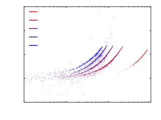
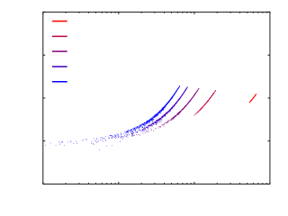
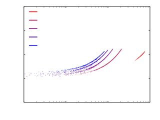
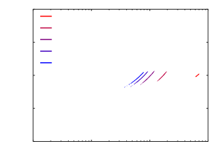
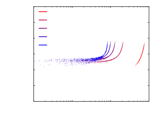
Figures 1 and 2 show the curvature functional $\Omega_{{\cal R}}^{{\cal D}}$. If an FLRW model is interpreted literally, then $\Omega_{{\cal R}}^{{\cal D}}$ is zero by assumption: $\Omega_{{\cal R}}^{{\cal D}}\equiv\Omega_{\mathrm{k}}=0$ in an EdS or $\Lambda$CDM model, and as was shown above, the overdensities cannot, at least pointwise, slow down to reach their turnaround epoch. For a more realistic, almost-FLRW model, Figs 1 and 2 show that both the EdS and $\Lambda$CDM models require very strong positive curvatures prior to turnaround. These $\Omega_{{\cal R}}^{{\cal D}}$–$H_{{\cal D}}$ relations are insensitive to particle resolution, and the ratios between the fundamental domain size $L_{\mathrm{box}}$, the averaging scale $L_{{\cal D}}$, the DTFE scale $L_{\mathrm{DTFE}}$, and the particle resolution scale $L_{N}$. For example, smaller QZA simulations with $L_{\mathrm{box}}=16L_{{\cal D}}=2L_{\mathrm{DTFE}}=2L_{N},N=64^{3}$ look visually almost indistinguishable from Figs 1 and 2.

It is clear in these figures that at any reasonable scale at which overdensities are normally thought to be able to collapse gravitationally, that is, from 2.5 to 40 Mpc/$h_{\mathrm{eff}}$, most spatial domains pass through a positive average curvature phase as they approach their turnaround epoch, that is, for the lowest values of $H_{{\cal D}}$ at the left of the panels. A striking feature of the plots is that at any given epoch, the relation between spatial curvature and expansion rate is mostly quite tight, especially at high expansion rates and early times. There is increasing scatter in the relation, mostly at lower values of $H_{{\cal D}}$, $L_{{\cal D}}=40$ Mpc/$h_{\mathrm{eff}}$ $\Lambda$CDM panel, in which turnaround is not reached. In Sect. 4.4 below, the ways that the $\Omega_{{\cal R}}^{{\cal D}}$–$H_{{\cal D}}$ relation could be used numerically or observationally are briefly discussed.

Figure 5: Averaged kinematical backreaction functional $\Omega_{{\cal Q}}^{{\cal D}}$ versus matter density functional $\Omega_{\mathrm{m}}^{{\cal D}}$, for domains in which the expansion parameter $H_{D}$ at the final time pre-turnaround time step satisfies $|H_{D}|<1$ km/s/Mpc, for an almost-EdS model, from top to bottom for $L_{{\cal D}}=2.5,10,40$ Mpc/$h_{\mathrm{eff}}$, respectively. A red line indicates $\Omega_{\mathrm{m}}^{{\cal D}}+\Omega_{{\cal Q}}^{{\cal D}}=0$. The region below/left of this line correspond to negative curvature ($\Omega_{{\cal R}}^{{\cal D}}>0$). The distributions of $(\Omega_{\mathrm{m}}^{{\cal D}},\Omega_{{\cal Q}}^{{\cal D}})$ pairs are clearly separated from the negative curvature region.

Figure 6: Averaged kinematical backreaction functional $\Omega_{{\cal Q}}^{{\cal D}}$ versus matter density functional $\Omega_{\mathrm{m}}^{{\cal D}}$, as in Fig. 5, for an almost-$\Lambda$CDM model, $L_{{\cal D}}=2.5$ Mpc/$h_{\mathrm{eff}}$ (top) and $10$ Mpc/$h_{\mathrm{eff}}$ (bottom); no turnaround occurs for $L_{{\cal D}}=40$ Mpc/$h_{\mathrm{eff}}$. The distributions of $(\Omega_{\mathrm{m}}^{{\cal D}},\Omega_{{\cal Q}}^{{\cal D}})$ pairs are clearly separated from the negative curvature region, which is bounded conservatively to lie to the left/below the diagonal red line, since $\Omega_{\Lambda}^{{\cal D}}\,\lower 2.58334pt\hbox{$\buildrel<\over{\sim}$}\,0.7$ (see Eq. (3.31)).

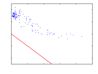
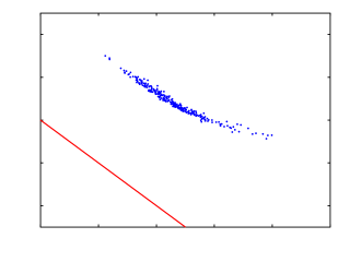
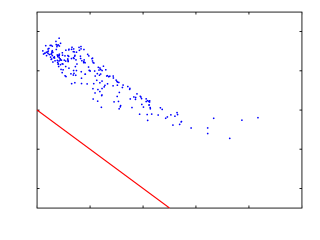
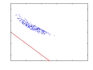
The curvatures for the domains at low $H_{{\cal D}}$ tend generally to approach the range $\Omega_{{\cal R}}^{{\cal D}}\sim-5$, which includes the EdS special case critical value of $\Omega_{{\cal R}}^{{\cal D}}=-5\alpha^{2}$, derived above in Eq. (3.19). An exception is the lowest panel of Fig. 2, for $L_{{\cal D}}=40$ Mpc/$h_{\mathrm{eff}}$, in which strong positive curvatures are not seen, because turnaround is not reached. In the simulation shown, the lowest expansion parameter $H_{{\cal D}}$ is $H_{{\cal D}}\sim 30$ km/s/Mpc at $t=13.8$ Gyr.

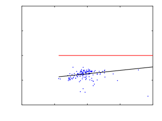
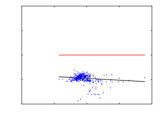
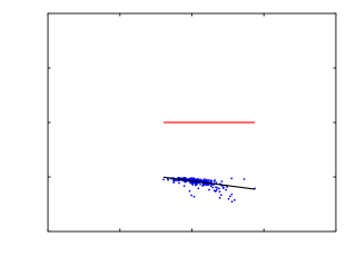
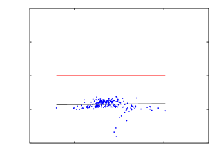
How close do the turnaround curvatures approach the EdS special case of $\Omega_{{\cal R}}^{{\cal D}}=-5\alpha^{2}$ given in Eq. (3.19)? Figures 3 and 4 are restricted to domains shown at the times when they are closest to turnaround, that is, with absolute values of $H_{{\cal D}}$ selected to satisfy $|H_{{\cal D}}|<1$ km/s/Mpc. The EdS special case occurs when the second and third initial average invariants of the peculiar-expansion tensor, $\left\langle{{{\mathrm{II}}}_{\mathbf{i}}}\right\rangle_{{\cal I}}$ and $\left\langle{{{\mathrm{III}}}_{\mathbf{i}}}\right\rangle_{{\cal I}}$, are zero. The latter is typically weaker than the former, so here we only show the behaviour with respect to the former, $\left\langle{{{\mathrm{II}}}_{\mathbf{i}}}\right\rangle_{{\cal I}}$. Robust linear fits [62, 63] to the $\Omega_{{\cal R}}^{{\cal D}}(\left\langle{\mathrm{II}}\right\rangle_{\cal D})$ relation are shown in the figures, and the zero points $\Omega_{{\cal R}}^{{\cal D}}({\mathrm{II}}=0)$ and their uncertainties are given in Table 2.

These ${\mathrm{II}}$ zero-point estimates of $\Omega_{{\cal R}}^{{\cal D}}$ are much closer to the $\Omega_{{\cal R}}^{{\cal D}}=-5\alpha^{2}$ special case than to the flatness assumed in an exact EdS or $\Lambda$CDM model, keeping in mind that $\alpha^{2}$ is close to unity at early epochs and can drop to about $0.5$ at late times in the EdS case, and close to unity at all times in the $\Lambda$CDM case. There is some scatter in $\Omega_{{\cal R}}^{{\cal D}}$ in Figs 3 and 4, even when $\left\langle{\mathrm{II}}\right\rangle_{\cal D}$ is close to zero, in particular due to the role of the third invariant $\left\langle{\mathrm{III}}\right\rangle_{\cal D}$, which we have not restricted in this analysis. The average values and scatter of $\Omega_{{\cal R}}^{{\cal D}}$, independent of the values of the initial invariants, are given in Table 4 using both non-robust and robust statistics. The value $\Omega_{{\cal R}}^{{\cal D}}=-5$ is not a statistical outlier for any of the three EdS distributions. Thus, for $\alpha\approx 1$, the EdS ${{{\mathrm{II}}}_{\mathbf{i}}}=0,{{{\mathrm{III}}}_{\mathbf{i}}}=0$ case gives a turnaround curvature that characterises the curvature distributions to first order. The $\Lambda$CDM distributions should not be expected to be identical to those for the EdS case, but they are not very different, apart from turnaround not being achieved for $L_{{\cal D}}=40$ Mpc/$h_{\mathrm{eff}}$.

A more direct comparison with the special analytical case is provided in Table 3, showing zero-point estimates of $\Delta_{{\cal R}}^{{\cal D}}$, in which the part of $\Omega_{{\cal R}}^{{\cal D}}$ due to growth function derivatives is removed (Eq. (3.22)). In the largest scale almost-EdS case and the smallest scale almost-$\Lambda$CDM case, the numerical estimates of the $\Delta_{{\cal R}}^{{\cal D}}$ zero point are statistically indistinguishable from the expected value of $-6$, but this is most likely a coincidence, as indicated by the other three estimates, which are inconsistent with $-6$ by up to about $0.5$ in ‘$\Omega$’ dimensionless units. Given the wide vertical scatter in Figs 3 and 4, summarised numerically in Table 4, and the simple fitting procedure adopted here, it is unsurprising that the agreement with the expected value is only approximate. The initial power spectrum is generic, and not intended to directly test the special $\left\langle{{{\mathrm{II}}}_{\mathbf{i}}}\right\rangle_{\cal D}=0,\left\langle{{{\mathrm{III}}}_{\mathbf{i}}}\right\rangle_{\cal D}=0$ case.

Figure 7: Curvature deviation parameter $\varepsilon$ as a function of expansion rate $H_{{\cal D}}$, as in Fig. 1, for the almost-EdS model. The vertical axis ranges vary from top to bottom panels (different $L_{{\cal D}}$ scales); the same ranges are used in Fig. 8.

Figure 8: Curvature deviation parameter $\varepsilon$ as a function of expansion rate $H_{{\cal D}}$, as in Fig. 7, for the almost-$\Lambda$CDM model.

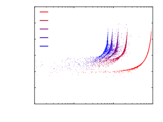
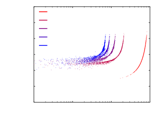
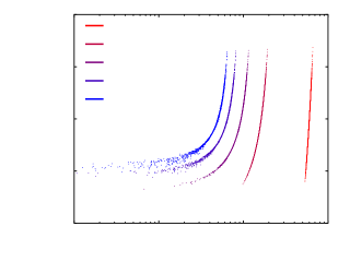
Overall, it is overwhelmingly clear in Figs 3 and 4 and Table 4 that turnaround is almost always associated with a strong positive average curvature. We further quantify this as follows.

Table 5 lists the fractions of domains which have negative or zero curvature. No such domains were found in any of the cases simulated. The total numbers of domains listed in Table 5 give an estimate of an upper limit to the frequency of occurrence of non-positive curvature at turnaround in the almost-EdS and almost-$\Lambda$CDM models. In order to increase the significance of the limit, we performed 29 additional independent $N=256^{3}$ realisations, each with the same parameters as the original. None of the domains had $\Omega_{{\cal R}}^{{\cal D}}\geq 0$ at turnaround. Thus, we estimate 99% numerical upper limits on the probability of a domain on these scales not having positive curvature at turnaround as $P=0.0002$ in the almost-EdS case (23125 domains reaching turnaround) and $P=0.0003$ in the almost-$\Lambda$CDM case (14526 domains). We estimate this upper limit by assuming that on average, $\bar{\mu}=5$ domains should have zero or negative curvature at turnaround out of the full sample reaching turnaround, but zero were detected due to random selection according to a Poisson distribution of mean $\bar{\mu}$. It is clearly very rare for a domain to be able to collapse in the average sense without having positive 3-Ricci curvature.

In the generalisation from pointwise collapse to average collapse in a domain, the expansion variance term appears in Eq. (2.5), and is usually combined with the shear scalar in the kinematical backreaction (Eq. (2.6)). To see how this could, in principle, allow a domain to reach the turnaround epoch in an averaged sense despite being spatially flat or negatively curved, the Hamiltonian constraint at turnaround, Eq. (3.25), can be rewritten

$$\Omega_{{\cal R}}^{{\cal D}}\geq 0\, \Leftrightarrow\,\left(\Omega_{\mathrm{m}}^{{\cal D}}+\Omega_{{\cal Q}}^{{\cal D}}+\Omega_{\Lambda}^{{\cal D}}\right)\leq 0\,.$$ (3.31)

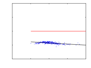
Figures 5 and 6 show the $\Omega_{\mathrm{m}}^{{\cal D}}$–$\Omega_{{\cal Q}}^{{\cal D}}$ relation for domains near turnaround. Since $\Omega_{\Lambda}^{{\cal D}}$ is low compared to $\Omega_{\mathrm{m}}^{{\cal D}}+\Omega_{{\cal Q}}^{{\cal D}}$ in these diagrams, a conservative bound for negative curvature is shown in both figures. Reaching zero or negative curvature would require a domain’s position in one of these diagrams to lie just at or to the left of/below the $\Omega_{\mathrm{m}}^{{\cal D}}+\Omega_{{\cal Q}}^{{\cal D}}=0$ line in Fig. 5, or somewhat to the left of/below the corresponding line in Fig. 6 after taking into account the value of $\Omega_{\Lambda}^{{\cal D}}$ for the domain.

The bands of points in Figs 5 and 6 give the impression that a selection criterion in $\Omega_{\mathrm{m}}^{{\cal D}}+\Omega_{{\cal Q}}^{{\cal D}}$ or $\Omega_{{\cal R}}^{{\cal D}}$ was applied in selecting the points. This is true only indirectly, in the sense that the points represent domains at pre-turnaround epochs when $|H_{{\cal D}}|<1$ km/s/Mpc. In other words, selecting for the turnaround epoch effectively makes a selection for spatial curvature to lie in a band not too far from the EdS special case of $\Omega_{{\cal R}}^{{\cal D}}=-5\alpha^{2}$.

4 Discussion

4.1 Foliation, gauge and vorticity

Are any of the results above gauge dependent? Proposition 1 (Sect. 1) and the definitions in Sect. 2.1 are given in terms of a foliation given certain assumptions restricting the allowed spacetimes. Defining a hypersurface orthogonal to the fluid flow provides a physical definition, so the hypersurfaces are gauge independent. The quantities of interest are scalars, which are invariant (coordinate independent). Choosing a different gauge to study the same quantities on the same spatial hypersurface would complicate the calculations, but could not modify the results unless the use of the new gauge change imposed additional constraints that modified the metric. Thus, the results presented here are not gauge dependent. If the EdS and $\Lambda$CDM models are interpreted as strictly FLRW models, with strictly flat spatial sections, then the relativistic forbidding of gravitational collapse cannot be avoided by gauge-dependence arguments. Similar reasoning applies to the plane-symmetric subcase.

In the almost-FLRW numerical QZA modelling in which curvature is allowed to vary above and below zero on any given spatial hypersurface and averages in Lagrangian domains are studied, gauge dependence is again not an issue (provided, again, that no restrictions are imposed by a gauge transformation), but foliation dependence could, in principle, be significant. Buchert, Mourier & Roy [64] argue that volume would differ by a factor of the order of the mean Lorentz factor $\gamma$ relating the fluid rest frame to an alternative reference frame. If the latter is that of a best-fit FLRW model to observational data, then fluid velocities of the order of 200 km/s would yield changes in volume or volume-based functionals such as $\Omega_{{\cal R}}^{{\cal D}}$ by about $\gamma-1<10^{-6}$, that is, the tilt between vectors normal to the different foliations is negligible in the present context. See [64] for more details, including the role of vorticity, for which in Newtonian cosmology simulations, the vorticity scalar is generally found to be weaker than the shear scalar [e.g. 65, Fig. 10].

Table 6: Software git commit hash that differs from Table 1; used for Fig. 9.

package, URL	git commit hash
ramses-scalav	14bfebd
https://bitbucket.org/broukema/ramses-scalav

Figure 9: Comoving domain pseudo-curvature functional $\Omega_{k}^{{\cal D}}$ versus expansion rate $H_{{\cal D}}$, from non-relativistic $N$-body simulations ($N$-body initial conditions) for a CMB-normalised almost-EdS model. From top to bottom panels: averaging scales $L_{{\cal D}}=2.5,10,40$ Mpc/$h_{\mathrm{eff}}$, respectively, where $L_{\mathrm{box}}=16L_{{\cal D}}=64L_{\mathrm{DTFE}}=128L_{N}$ and $N=128^{3}$ particles. Colours and ranges are as in Fig. 1.

4.2 Newtonian $N$-body equivalents

Adamek et al. [66] argue that a change in the choice of foliation, which necessarily changes the choice of gauge, can affect parameters calculated in relation to backreaction by 2–3 orders of magnitude. In this discussion, we do not try to resolve the apparent disagreement between the claims of [64] and [66].

Instead, we consider the equivalent of the curvature–expansion-rate relation in a conventional $N$-body simulation and compare it with our RZA-based curvature–expansion-rate relation. We need a ‘pseudo-curvature’ parameter that can be estimated from Newtonian $N$-body simulations and interpreted as what would constitute curvature in the relativistic case. We replace Eq. (2.6) by its Newtonian equivalent [45, Eq. (6)]; we retain the equivalent of Eq. (3.24), that is,

$$\Omega_{{\cal Q}}^{{\cal D}}:=-{\cal Q}_{{\cal D}}/(6H^{2})\;,$$ (4.1)

using the expansion rate $H$ of the reference model; and in a slight variation of the approach in ref. [45, II.D], we use the Newtonian averaged Hamiltonian constraint [45, Eq. (17)] to define a Newtonian pseudo-curvature parameter

$$\Omega_{k}^{{\cal D}}:=1-\Omega_{\mathrm{m}}^{{\cal D}}-\Omega_{\Lambda}^{{\cal D}}-\Omega_{{\cal Q}}^{{\cal D}}\;.$$ (4.2)

(We run the simulations for an EdS reference model, so $\Omega_{\Lambda}^{{\cal D}}\equiv 0$ in this case.) We use the same numerical method as above, apart from switching ramses-scalav from RZA integration to $N$-body mode, as indicated using the software version listed in Table 6. This method provides an approximate comparison with the above results, with some differences. The definitions in this section apply to the conventional Newtonian foliation, which (i) is not fluid-orthogonal. Two other differences with the RZA method are that (ii) vorticity is not set to zero (so the foliation is not irrotational), and (iii) the domains for calculating the invariants of the peculiar expansion tensor and averaging have fixed comoving-FLRW spatial boundaries, not Lagrangian spatial boundaries.

We performed these simulations for the EdS reference model and show the results in Fig. 9. Comparing these to Fig. 1 and keeping in mind the three differences in the method, the curvature–expansion-rate relations appear to be broadly consistent between the two figures. The use of comoving-FLRW boundaries to define domains prevents any domain from collapsing to zero size and weakens the ability of a domain to achieve turnaround (since turnaround in this case requires a larger spatial region than the original Lagrangian region to have slowed down to momentary mean staticity in physical spatial coordinates). It is thus unsurprising that the rather sharply defined relations pointing towards $\Omega_{{\cal R}}^{{\cal D}}\sim-5$ at turnaround in Fig. 1 are less apparent in Fig. 9. The intermediate scale simulation, for $L_{{\cal D}}=10$ Mpc/$h_{\mathrm{eff}}$, best suggests an approach towards $\Omega_{{\cal R}}^{{\cal D}}\sim-5$ at turnaround ($H_{{\cal D}}\rightarrow 0$ km/s/Mpc), but the use of comoving-FLRW boundaries appears to lead to fuzzier curvature–expansion-rate relations than for Lagrangian boundaries. For the largest scale, $L_{{\cal D}}=40$ Mpc/$h_{\mathrm{eff}}$, turnaround is not reached for this comoving domain size. The smaller scale, $L_{{\cal D}}=2.5$ Mpc/$h_{\mathrm{eff}}$, has a broad scatter of domains consistent with approaching turnaround at curvatures that are mostly positive. It would seem reasonable to attribute the other differences (such as straight versus curved relations) to the different choices of foliation and vorticity. Overall, the tendency to require positive average spatial cuvature to reach turnaround remains present in these Newtonian pseudo-curvature calculations as shown in Fig. 9, but is less sharply defined than in the RZA calculations.

4.3 The curvature-induced deviation $\varepsilon$

The relations in Figs 1 and 2 indicate methods both of calibrating cosmological structure formation simulations that claim to be fully relativistic, and, in principle, of being measured observationally. What possible avenues could there be for measuring $\Omega_{{\cal R}}^{{\cal D}}$ in a given spatial domain? Here, we introduce a dimensionless ‘curvature-induced deviation’ variable $\varepsilon$ defined for non-zero curvature that depends both on the curvature and on the averaging scale. We express the average 3-Ricci curvature for non-zero curvature as a typical curvature radius $L_{{\cal R}}^{{\cal D}}$ (in physical units) with a value that is real for positive curvature and imaginary for negative curvature,

$$L_{{\cal R}}^{{\cal D}}:=\left(H_{\mathrm{eff}}\,\sqrt{-\Omega_{{\cal R}}^{{\cal D}}}\right)^{-1}\,,$$ (4.3)

We consider a length $l$ over which to estimate the deviation of a pair of straight lines (spatial geodesics at constant $t$ in the foliation) that at one location are locally parallel. We set $l=a_{{\cal D}}L_{{\cal D}}$, the approximate average physical size of a domain (the cube root of the volume) at the averaging scale $L_{{\cal D}}$, where as above, $L_{{\cal D}}$ is expressed in effective-model comoving units. This approximatoin is valid to first order in $L_{{\cal R}}^{{\cal D}}$. The curvature-induced deviation’s functional dependence is

$$\varepsilon(\left\langle{\cal R}\right\rangle_{\cal D},l) \equiv\varepsilon(\Omega_{{\cal R}}^{{\cal D}},H_{\mathrm{eff}},a_{{\cal D}},L_{{\cal D}})\equiv\varepsilon(L_{{\cal R}}^{{\cal D}},a_{{\cal D}},L_{{\cal D}}).$$ (4.4)

This functional is designed to measure the difference of an arc length on the constant foliation time hypersurface, interpreted as having constant curvature $\left\langle R\right\rangle_{\cal D}$, from the corresponding arc length in a corresponding flat spatial section, at a distance corresponding to the averaging scale $L_{{\cal D}}$ (again in comoving effective units, as for $L_{{\cal D}}$ throughout this work), and normalised by that same distance $L_{{\cal D}}$,

$$\varepsilon :=\frac{1}{a_{{\cal D}}\,L_{{\cal D}}}\left(L_{{\cal R}}^{{\cal D}}\sin\frac{a_{{\cal D}}\,L_{{\cal D}}}{L_{{\cal R}}^{{\cal D}}}-a_{{\cal D}}\,L_{{\cal D}}\right)$$

$$=-\frac{1}{6}\,\left(a_{{\cal D}}\,H_{\mathrm{eff}}\,L_{{\cal D}}\right)^{2}\Omega_{{\cal R}}^{{\cal D}}+\ldots\,,$$ (4.5)

in which the third-order Taylor expansion for $\sin$ (or $\sinh$) should be used for numerical stability in nearly flat domains ($|\Omega_{{\cal R}}^{{\cal D}}|\ll 1$; in exactly flat domains, $\varepsilon:=0$), and positive curvature corresponds to negative $\Omega_{{\cal R}}^{{\cal D}}$ and negative $\varepsilon$. For example, two locally parallel spatial geodesics separated by 1 Mpc should be separated by about $(1+\varepsilon)$ Mpc after being extended by a distance of $L_{{\cal D}}$. Time-integrated dynamical quantities will differ from flat-space calculations by integrals including $\varepsilon$ terms.

Figures 7 and 8 show the curvature-induced deviation $\varepsilon$. The amplitudes of this effect range from about $10^{-7}$ at the $L_{{\cal D}}=2.5$ Mpc/$h_{\mathrm{eff}}$ scale (top panels) up to a little above $10^{-5}$ at the largest comoving scale, $L_{{\cal D}}=40$ Mpc/$h_{\mathrm{eff}}$ (bottom panels). This can be interpreted using the rightmost expression in Eq. (4.5), since an increase in $L_{{\cal D}}^{2}$ by a factor of 16 approximately corresponds to the increase in the typical magnitudes of $\varepsilon$ from the top to middle panels in these two figures. The increase is weaker in shifting to the largest scale (bottom panels). In particular, the bottom panel in Fig. 8 shows a scale in the almost-$\Lambda$CDM model at which turnaround is not reached, so only weak positive curvature results and the curvature-induced deviation $\varepsilon$ is correspondingly weak.

Given that the $\Lambda$CDM model is a fair observational proxy, the lower two panels of Fig. 8 indicate that spatial (constant $t$ for our foliation) geodesics that in strict $\Lambda$CDM are assumed to be parallel must, in a relativistic almost-$\Lambda$CDM model including structure formation, converge or diverge at about the $10^{-6}$ to $10^{-5}$ level after passing through a typical turnaround domain. Observations are performed on the past light cone, so the curvature-induced deviation $\varepsilon$ defined here in Eq. (4.5) on a constant-$t$ hypersurface in the fluid-orthogonal irrotational foliation will correspond to a somewhat different deviation of observers’ null geodesics on the light cone. It is unlikely that the amplitude of deviation should be significantly weaker on the light cone than in the spatial hypersurface. Thus, observational analyses of dense regions of the cosmic web made under the assumption of an FLRW metric, without taking into account spatially varying curvature, should be relativistically inaccurate at about this level. While weak lensing surveys take spatial curvature into account, as modelled by linear perturbation theory [e.g. 67], there are many cosmological observational analyses that do not, and instead, algebraically assume that turnaround-epoch spatial curvature is insignificant. For example, the baryon acoustic oscillation discovery papers [4, 5] do not appear to assume any deviation from a strict FLRW model, whether by weak lensing or by turnaround-epoch lensing; global curvature constraint estimates, such as that of [6], do not appear to take into account any non-FLRW effects; the main analyses of [7] and [8], leaving aside gravitational weak lensing analyses, adopt a flat FLRW model. Here, we have shown that the inaccuracy of these assumptions should lie at roughly the $10^{-6}$ to $10^{-5}$ level when passing through a single turnaround domain. A potential application of the non-perturbative RZA approach would be to extend standard weak lensing methods beyond first and second order perturbation theory. In the new generation of surveys, detecting turnaround-epoch lensing effects (geodesic deviations) is likely to be difficult, but should in principle provide a test of precise, accurate cosmology.

These low values of $\varepsilon$ do not necessarily contradict the recently emerged negative average curvature hypothesis ([68, 69, 70, 71, 72, 73, 48, 39, 74, 75, 76, 77, 78, 79, 80, 47, 81, 82, 83, 59, 84, 85, 86, 87, 88, 89, 90, 91]) of explaining dark energy as a misinterpretation of (non-relativistic fit to) cosmological observations. The curvature deviation $\varepsilon$ indicates how much spatial geodesics should converge or diverge, not how much expansion rates should be spatially inhomogeneous. It is already known observationally that the BAO scale is inhomogeneous when using the $\Lambda$CDM model as a proxy to interpret the luminous red galaxy distribution in the Sloan Digital Sky Survey ([92, 93]; see [94] for interpretation in terms of an inhomogeneous model and [95, 96] for related analyses). The main order of magnitude observational argument supporting the emergent negative average curvature hypothesis is the void peculiar expansion rate, that is, the ratio of the peculiar velocities of galaxies falling out of voids to the void sizes, which is typically of a few tens of km/s/Mpc – a substantial fraction of the Hubble–Lemaître constant [77, 29].

Non-perturbative work on the recently emerged negative average curvature hypothesis shows in more detail how the curvature functional $\Omega_{{\cal R}}^{{\cal D}}$ reveals negative curvature in a void and positive curvature in an overdensity. Using a Szekeres model to model a local void and nearby overdensity and domains that are spheres of radius 5 Mpc, [83, Fig. 2, bottom-right panel] showed negative curvature in the (central) void and positive curvature in the overdensity (lying at $-40$ Mpc $\,\lower 2.58334pt\hbox{$\buildrel<\over{\sim}$}\,z\,\lower 2.58334pt\hbox{$\buildrel<\over{\sim}$}\,-20$ Mpc). The results presented in this work are consistent with the conclusion of [83] that for non-perturbative, non-linear calculations, curvature associated with structure formation is highly inhomogeneous, and of an order of magnitude at least as great as that of the FLRW density parameter $\Omega_{\mathrm{m}}$.

4.4 New GR test: the $\Omega_{{\cal R}}^{{\cal D}}$–$H_{{\cal D}}$ relation

The turnaround-epoch positive spatial curvature requirement is not overtly coded into the Euclidean spatial geometry of a Newtonian simulation. In terms of linear perturbation theory interpretations, the Newtonian-gauge gravitational potential gradient matches spatial curvature to first order. In this sense, it could be argued that the requirement is present implicitly in an approximate sense. However, such an interpretation does not account for the fact that vector arithmetic is, in principle, no longer globally justified in the presence of positive (or negative) spatial curvature – tangent and cotangent spaces of vectors and 1-forms at individual spacetime events have to be related to each other via a connection, typically the covariant derivative.

Nevertheless, [97, 98, 99, 100] have proposed the ‘Newtonian motion (Nm)’ gauge formalism, which derives diffeomorphisms (a ‘dictionary’) that under appropriate conditions relate Newtonian $N$-body simulations to general-relativistic spacetime. The authors argue that the approximations used are cosmologically accurate. The role of spatial curvature is implicitly described in [100, Sect. 5.2]. A useful crosscheck between the Nm formalism and the QZA formalism (also used by [61] in the plane-symmetric case) would be to evaluate the $\Omega_{{\cal R}}^{{\cal D}}$–$H_{{\cal D}}$ relation on a fluid-orthogonal, irrotational foliation of a Newtonian cosmological $N$-body simulation and check the resulting values against the scalar averaging results found in this work. The two approaches make differing simplifications, so consistency of the results would suggest that the simplifications do not have strong effects. Similarly, crosschecks against the partially relativistic cosmological simulation code gevolution [101] and the fully relativistic cosmological simulation packages used within the Einstein Toolkit [102, 103, (et)] would be useful. Differences between these would have to be understood. In the subcases in which RZA is exact, such as the plane-symmetric case, the simplicity of the RZA approach would potentially provide a good test for calibrating the computational accuracy of gevolution and et.

In principle, it should be possible to test the $\Omega_{{\cal R}}^{{\cal D}}$–$H_{{\cal D}}$ relation observationally, as a new test of the Einstein equation. In practice, this is likely to be very difficult.

4.5 Geometrical dark matter

Earlier discussion of the role of exact relativistic solutions has pointed out the difference between these and the perturbed FLRW approach, arguing that there is effectively a ‘general-relativistic dark matter’ component associated with gravitational collapse on cosmologically relevant scales, using Tolman–Lemaître–Bondi models [104, 105, 106], the quasi-spherical Szekeres model [106, 107], and Szekeres Class-II models [108], though without a clear focus on the role of pointwise or domain averaged positive curvature. The expectation that there is an effective form of general-relativistic dark matter has been discussed in the more general context of scalar averaging by, in particular, [109] and [33], but without making calculations based on generic realisations of a standard initial power spectrum of density perturbations. [33] coined the term ‘kinematical dark matter’, suggesting that the shear scalar, on small scales, was the most likely explanation to provide a kinematical dark matter contribution to the usual observational interpretation of dark matter, through its role in the Raychaudhuri equation, especially at the later phases of gravitational collapse. Equations (2.1) and (2.5) show that at late phases, a higher compression rate, that is, a greater value of $|H_{D}|$ during the $H_{D}<0$ post-turnaround phase, would also be contributed by the shear scalar to a late-phase kinematical dark matter effect. In this work, we focussed instead on the turnaround epoch and made calculations based on a standard initial power spectrum of Gaussian fluctuations, finding that at turnaround, positive curvature much more frequently plays the dominant role in gravitational collapse, at least near the turnaround epoch, rather than kinematical backreaction, which is the net effect of expansion variance and the shear scalar together. Simultaneously to the present work, [61] showed that in the plane-symmetric case, kinematical backreaction becomes stronger in amplitude than curvature during the post-turnaround phase, rather than remaining at its turnaround value of one-fifth of the latter in absolute value (see (3.27)).

Since turnaround-epoch positive spatial curvature is a geometrical phenomenon, not just dynamical, it should, in principle, contribute to weak lensing effects. It could well play a role in modifying the usual calculations of weak lensing effects – again, possibly substituting for some of the present role of FLRW ‘perturbative’ dark matter. Since the effective ‘source’ of dark matter in this sense is positive curvature rather than kinematical backreaction, we suggest ‘geometrical dark matter’ as an appropriate term when positive curvature in the averaged Hamiltonian constraint is the dominating dark-matter–like relativistic effect. Whether or not turnaround-epoch positive spatial curvature constitutes a new contribution to weak lensing that justifies the term ‘geometrical dark matter’ will be a useful question for further work in this field. The discussion and figure in Sect. 4.2 suggest that conventional $N$-body simulations would be sufficient to provide an approximate answer to this question, although the use of relativistic simulations and/or RZA calculations would provide a relativistically more accurate answer.

5 Conclusion

It is now clear, both from a general argument (Sect. 3.1, Proposition 1) and from an exact cosmological solution close to an EdS or $\Lambda$CDM reference model (Sect. 3.2), that the interpretation of the $\Lambda$CDM model as only containing literally 3-Ricci–flat spatial domains, rather than interpreting it as an almost-FLRW model with inhomogeneous curvature, would forbid almost all formation of dense structures. This is because inhomogeneities that are initially expanding in terms of physical distances cannot sufficiently slow down their expansion (isotropically and pointwise) to pass through the turnaround epoch if zero spatial curvature is strictly imposed in a fluid-orthogonal foliation.

We thus considered the more reasonable hypothesis that relativistic constraints permit a standard initial power spectrum of Gaussian random density fluctuations that evolves according to the growing mode. By using the relativistic Zel’dovich approximation, we first showed that for null initial average second and third peculiar-expansion tensor invariants ($\left\langle{{{\mathrm{II}}}_{\mathbf{i}}}\right\rangle_{{\cal I}}(\theta^{i}_{j})=0$, $\left\langle{{{\mathrm{III}}}_{\mathbf{i}}}\right\rangle_{{\cal I}}(\theta^{i}_{j})=0$) in an almost-EdS model, a critical value of the curvature functional $\Omega_{{\cal R}}^{{\cal D}}=-5\alpha^{2}$ (where $\alpha:={H}/{H_{\mathrm{eff}}}$ and $0.5\,\lower 2.58334pt\hbox{$\buildrel<\over{\sim}$}\,\alpha^{2}\,\lower 2.58334pt\hbox{$\buildrel<\over{\sim}$}\,1$; alternatively, we can write this as $\Omega_{{\cal R}}^{{\cal D}}=-5$ for normalisation using the EdS expansion rate instead of the effective expansion rate), corresponding to positive spatial scalar curvature, must occur in a domain as it passes through the turnaround epoch (Sect. 3.3.1).

For the more general case of standard initial conditions, using kinematical backreaction evolution as modelled by the RZA and implemented using the inhomog library (QZA, Sect. 2.4.2), we showed that almost-EdS and almost-$\Lambda$CDM models give values of $\Omega_{{\cal R}}^{{\cal D}}$ at turnaround corresponding to positive curvature and lying in a range that includes this critical value (Sect. 3.3.2, Figs 1–6, Tables 2–4). In the context where FLRW cosmological parameters are believed to be approaching precision at the one percent level, and possibly also a similar level of accuracy, we find that neglecting strong turnaround-epoch curvature is unlikely to lead to signficant inaccuracies in standard flat-space cosmological $N$-body simulations and observational data analyses (Sect. 4, Figs 7, 8). The explicit inclusion of turnaround-epoch positive spatial curvature in the analysis of the upcoming generation of major extragalactic surveys would nevertheless, in principle, be useful as an improvement beyond the methods of linear perturbation theory.

References

- [1] A. Friedmann, Mir kak prostranstvo i vremya (The Universe as Space and Time). Petrograd: Academia, 1923.
- [2] G. Lemaître, Un Univers homogène de masse constante et de rayon croissant rendant compte de la vitesse radiale des nébuleuses extra-galactiques, Ann. de la Soc. Sc. de Brux. 47 (1927) 49–59.
- [3] H. P. Robertson, Kinematics and World-Structure, ApJ 82 (Nov., 1935) 284.
- [4] S. Cole, W. J. Percival, J. A. Peacock, P. Norberg, C. M. Baugh, C. S. Frenk, I. Baldry, J. Bland-Hawthorn, and et al., The 2dF Galaxy Redshift Survey: power-spectrum analysis of the final data set and cosmological implications, MNRAS 362 (Sept., 2005) 505–534, [astro-ph/0501174].
- [5] D. J. Eisenstein, I. Zehavi, D. W. Hogg, R. Scoccimarro, M. R. Blanton, R. C. Nichol, R. Scranton, H.-J. Seo, and et al., Detection of the Baryon Acoustic Peak in the Large-Scale Correlation Function of SDSS Luminous Red Galaxies, ApJ 633 (Nov., 2005) 560–574, [astro-ph/0501171].
- [6] J. Ryan, Y. Chen, and B. Ratra, Baryon acoustic oscillation, Hubble parameter, and angular size measurement constraints on the Hubble constant, dark energy dynamics, and spatial curvature, MNRAS 488 (Sep, 2019) 3844–3856, [arXiv:1902.03196].
- [7] C. L. Bennett, D. Larson, J. L. Weiland, N. Jarosik, G. Hinshaw, N. Odegard, K. M. Smith, R. S. Hill, and et al., Nine-year Wilkinson Microwave Anisotropy Probe (WMAP) Observations: Final Maps and Results, ApJSupp 208 (Oct., 2013) 20, [arXiv:1212.5225].
- [8] P. A. R. Ade, N. Aghanim, M. Arnaud, M. Ashdown, J. Aumont, C. Baccigalupi, A. J. Banday, R. B. Barreiro, and et al., Planck 2015 results. XIII. Cosmological parameters, A&A 594 (Sept., 2016) A13, [arXiv:1502.01589].
- [9] R. Durrer, Anisotropies in the cosmic microwave background: theoretical foundations., Helvetica Physica Acta 69 (Nov., 1996) 417–433, [astro-ph/9610234].
- [10] A. Krasiński, Inhomogeneous Cosmological Models. Cambridge, UK: Cambridge University Press, Nov., 2006.
- [11] J. A. Tyson, D. M. Wittman, J. F. Hennawi, and D. N. Spergel, LSST: a complementary probe of dark energy, Nucl. Phys. B Proc. Supp. 124 (July, 2003) 21–29, [astro-ph/0209632].
- [12] R. S. de Jong, O. Bellido-Tirado, C. Chiappini, E. Depagne, R. Haynes, D. Johl, O. Schnurr, A. Schwope, and et al., 4MOST: 4-metre multi-object spectroscopic telescope, in Ground-based and Airborne Instrumentation for Astronomy IV (I. S. McLean, S. K. Ramsay, and H. Takami, eds.), vol. 8446 of SPIE Conf. Ser. , p. 84460T, Sept., 2012. arXiv:1206.6885.
- [13] J. Richard, J. P. Kneib, C. Blake, A. Raichoor, J. Comparat, T. Shanks, J. Sorce, M. Sahlén, and et al., 4MOST Consortium Survey 8: Cosmology Redshift Survey (CRS), The Messenger 175 (Mar, 2019) 50, [arXiv:1903.02474].
- [14] M. Levi, C. Bebek, T. Beers, R. Blum, R. Cahn, D. Eisenstein, B. Flaugher, K. Honscheid, and et al., The DESI Experiment, a whitepaper for Snowmass 2013, ArXiv e-prints (Aug., 2013) [arXiv:1308.0847].
- [15] G.-B. Zhao, Y. Wang, A. J. Ross, S. Shandera, W. J. Percival, K. S. Dawson, J.-P. Kneib, A. D. Myers, and et al., The extended Baryon Oscillation Spectroscopic Survey (eBOSS): a cosmological forecast, MNRAS 457 (Apr., 2016) 2377–2390, [arXiv:1510.08216].
- [16] A. Refregier, A. Amara, T. D. Kitching, A. Rassat, R. Scaramella, and J. Weller, Euclid Imaging Consortium Science Book, ArXiv e-prints (Jan., 2010) [arXiv:1001.0061].
- [17] J. Delabrouille, P. de Bernardis, F. R. Bouchet, A. Achúcarro, P. A. R. Ade, R. Allison, F. Arroja, E. Artal, and et al, Exploring Cosmic Origins with CORE: Survey requirements and mission design, JCAP 2018 (Apr, 2018) 014, [arXiv:1706.04516].
- [18] G. de Zotti, G. Castex, J. Gonzalez-Nuevo, M. Lopez-Caniego, M. Negrello, Z.-Y. Cai, M. Clemens, J. Delabrouille, and et al., Extragalactic sources in Cosmic Microwave Background maps, JCAP 6 (June, 2015) 18, [arXiv:1501.02170].
- [19] G. de Zotti, J. Gonzalez-Nuevo, M. Lopez-Caniego, M. Negrello, J. Greenslade, C. Hernandez-Monteagudo, J. Delabrouille, Z.-Y. Cai, and et al., Exploring Cosmic Origins with CORE: Extragalactic sources in Cosmic Microwave Background maps, JCAP 2018 (Apr, 2018) 020, [arXiv:1609.07263].
- [20] H. Kodama and M. Sasaki, Cosmological Perturbation Theory, Progress of Theoretical Physics Supplement 78 (1984) 1.
- [21] J. S. Bagla and T. Padmanabhan, Cosmological N-body simulations., Pramana 49 (Aug, 1997) 161, [astro-ph/0411730].
- [22] R. Teyssier, Cosmological hydrodynamics with adaptive mesh refinement. A new high resolution code called RAMSES, A&A 385 (Apr., 2002) 337–364, [astro-ph/0111367].
- [23] V. Springel, The cosmological simulation code GADGET-2, MNRAS 364 (Dec., 2005) 1105–1134, [astro-ph/0505010].
- [24] T. Guillet and R. Teyssier, A simple multigrid scheme for solving the Poisson equation with arbitrary domain boundaries, Journal of Computational Physics 230 (June, 2011) 4756–4771, [arXiv:1104.1703].
- [25] T. Buchert and J. Ehlers, Averaging inhomogeneous Newtonian cosmologies., A&A 320 (Apr., 1997) 1–7, [astro-ph/9510056].
- [26] G. F. R. Ellis, relativistic cosmology., in General Relativity and Cosmology (R. K. Sachs, ed.), pp. 104–182, 1971.
- [27] G. F. R. Ellis, Republication of: Relativistic cosmology, General Relativity and Gravitation 41 (Mar., 2009) 581–660.
- [28] G. F. R. Ellis, R. Maartens, and M. A. H. MacCallum, Relativistic Cosmology. UK: Cambridge University Press, Mar., 2012.
- [29] B. F. Roukema, P. Mourier, T. Buchert, and J. J. Ostrowski, The background Friedmannian Hubble constant in relativistic inhomogeneous cosmology and the age of the Universe, A&A 598 (Feb., 2017) A111, [arXiv:1608.06004].
- [30] T. Buchert, On Average Properties of Inhomogeneous Fluids in General Relativity: Dust Cosmologies, Gen. Rel. Grav. 32 (Jan., 2000) 105–126, [gr-qc/9906015].
- [31] J. Ehlers, Beiträge zur relativistischen Mechanik kontinuierlicher Medien, Mainz Akademie Wissenschaften Mathematisch Naturwissenschaftliche Klasse 11 (1961).
- [32] J. Ehlers, Contributions to the relativistic mechanics of continuous media, General Relativity and Gravitation 25 (Dec., 1993) 1225–1266.
- [33] T. Buchert, C. Nayet, and A. Wiegand, Lagrangian theory of structure formation in relativistic cosmology II: average properties of a generic evolution model, PRD 87 (June, 2013) 123503, [arXiv:1303.6193].
- [34] E. Hubble, A Relation between Distance and Radial Velocity among Extra-Galactic Nebulae, Proc. Nat. Acad. Sci. 15 (Mar., 1929) 168–173.
- [35] G. Lemaître, Expansion of the universe, A homogeneous universe of constant mass and increasing radius accounting for the radial velocity of extra-galactic nebulæ, MNRAS 91 (Mar., 1931) 483–490.
- [36] G. F. R. Ellis, M. Bruni, and J. Hwang, Density-gradient-vorticity relation in perfect-fluid Robertson-Walker perturbations, PRD 42 (Aug., 1990) 1035–1046.
- [37] C. G. Tsagas, A. Challinor, and R. Maartens, Relativistic cosmology and large-scale structure, Phys.Rep. 465 (Aug., 2008) 61–147, [arXiv:0705.4397].
- [38] S. Magni, Backreaction and the Covariant Formalism of General Relativity, Master’s thesis, Facoltà di Scienze Matematiche, Fisiche e Naturali, Università degli studi di Pavia, 2011.
- [39] T. Buchert and S. Räsänen, Backreaction in Late-Time Cosmology, Ann. Rev. Nucl. Part. Sci. 62 (Nov., 2012) 57–79, [arXiv:1112.5335].
- [40] G. F. R. Ellis, Dynamics of Pressure-Free Matter in General Relativity, Journal of Mathematical Physics 8 (May, 1967) 1171–1194.
- [41] A. Krasiński, Geometry and topology of the quasiplane Szekeres model, PRD 78 (Sept., 2008) 064038, [arXiv:0805.0529].
- [42] E. Di Dio, M. Vonlanthen, and R. Durrer, Back reaction from walls, JCAP 2 (Feb., 2012) 036, [arXiv:1111.5764].
- [43] J. Adamek, E. Di Dio, R. Durrer, and M. Kunz, Distance-redshift relation in plane symmetric universes, PRD 89 (Mar., 2014) 063543, [arXiv:1401.3634].
- [44] P. Szekeres, A class of inhomogeneous cosmological models, Communications in Mathematical Physics 41 (Feb., 1975) 55–64.
- [45] T. Buchert, M. Kerscher, and C. Sicka, Back reaction of inhomogeneities on the expansion: The evolution of cosmological parameters, PRD 62 (Aug., 2000) 043525, [astro-ph/9912347].
- [46] T. Buchert and M. Ostermann, Lagrangian theory of structure formation in relativistic cosmology: Lagrangian framework and definition of a nonperturbative approximation, PRD 86 (July, 2012) 023520, [arXiv:1203.6263].
- [47] B. F. Roukema, Replacing dark energy by silent virialisation, A&A 610 (Feb., 2018) A51, [arXiv:1706.06179].
- [48] A. Wiegand and T. Buchert, Multiscale cosmology and structure-emerging dark energy: A plausibility analysis, PRD 82 (July, 2010) 023523, [arXiv:1002.3912].
- [49] E. Bertschinger, Multiscale Gaussian Random Fields and Their Application to Cosmological Simulations, ApJSupp 137 (Nov., 2001) 1–20, [astro-ph/0103301].
- [50] S. Prunet, C. Pichon, D. Aubert, D. Pogosyan, R. Teyssier, and S. Gottloeber, Initial Conditions For Large Cosmological Simulations, ApJSupp 178 (Oct., 2008) 179–188, [arXiv:0804.3536].
- [51] W. E. Schaap and R. van de Weygaert, Continuous fields and discrete samples: reconstruction through Delaunay tessellations, A&A 363 (Nov., 2000) L29–L32, [astro-ph/0011007].
- [52] R. van de Weygaert and W. Schaap, The Cosmic Web: Geometric Analysis, in Data Analysis in Cosmology (V. J. Martínez, E. Saar, E. Martínez-González, and M.-J. Pons-Bordería, eds.), vol. 665 of Lecture Notes in Physics, Berlin Springer Verlag, pp. 291–413, 2009. arXiv:0708.1441.
- [53] M. C. Cautun and R. van de Weygaert, The DTFE public software - The Delaunay Tessellation Field Estimator code, ArXiv e-prints (May, 2011) [arXiv:1105.0370].
- [54] M. B. Kennel, KDTREE 2: Fortran 95 and C++ software to efficiently search for near neighbors in a multi-dimensional Euclidean space, ArXiv e-prints (Aug., 2004) [physics/0408067].
- [55] M. Kasai, An analytical approximation of the growth function in Friedmann-Lema\ître universes, ArXiv e-prints (Dec., 2010) [arXiv:1012.2671].
- [56] S. Bildhauer, T. Buchert, and M. Kasai, Solutions in Newtonian cosmology - The pancake theory with cosmological constant, A&A 263 (Sept., 1992) 23–29.
- [57] P. J. E. Peebles, Tests of cosmological models constrained by inflation, ApJ 284 (Sept., 1984) 439–444.
- [58] V. Sahni and A. Starobinsky, The Case for a Positive Cosmological -Term, Int. J. Mod. Phys. D 9 (2000) 373–443, [astro-ph/9904398].
- [59] K. Bolejko, Emergence of spatial curvature, ArXiv e-prints (July, 2017) [arXiv:1707.01800].
- [60] K. Bolejko, Relativistic numerical cosmology with silent universes, Class. Quant. Gra. 35 (Jan., 2018) 024003, [arXiv:1708.09143].
- [61] Q. Vigneron and T. Buchert, Dark matter from backreaction? Collapse models on galaxy cluster scales, Classical and Quantum Gravity 36 (Sep, 2019) 175006, [arXiv:1902.08441].
- [62] H. Theil, A rank-invariant method of linear and polynomial regression analysis, Nederl. Akad. Wetensch., Proc. 53 (1950) 386–392.
- [63] P. K. Sen, Estimates of the regression coefficient based on Kendall’s tau, J. Amer. Stat. Assoc. 63 (1968) 1379–1389.
- [64] T. Buchert, P. Mourier, and X. Roy, Cosmological backreaction and its dependence on spacetime foliation, Classical and Quantum Gravity 35 (Dec., 2018) 24LT02, [arXiv:1805.10455].
- [65] F. Bernardeau and R. van de Weygaert, A new method for accurate estimation of velocity field statistics, MNRAS 279 (Mar., 1996) 693, [astro-ph/9508125].
- [66] J. Adamek, C. Clarkson, D. Daverio, R. Durrer, and M. Kunz, Safely smoothing spacetime: backreaction in relativistic cosmological simulations, Class. Quant. Gra. 36 (Jan, 2019) 014001, [arXiv:1706.09309].
- [67] M. Bartelmann and P. Schneider, Weak gravitational lensing, Phys.Rep. 340 (Jan, 2001) 291–472, [astro-ph/9912508].
- [68] S. Räsänen, Accelerated expansion from structure formation, JCAP 11 (Nov., 2006) 003, [astro-ph/0607626].
- [69] Y. Nambu and M. Tanimoto, Accelerating Universe via Spatial Averaging, ArXiv e-prints (July, 2005) [gr-qc/0507057].
- [70] T. Kai, H. Kozaki, K. Nakao, Y. Nambu, and C. Yoo, Can Inhomogeneities Accelerate the Cosmic Volume Expansion?, Progress of Theoretical Physics 117 (Feb., 2007) 229–240, [gr-qc/0605120].
- [71] S. Räsänen, Evaluating backreaction with the peak model of structure formation, JCAP 4 (Apr., 2008) 026, [arXiv:0801.2692].
- [72] J. Larena, J.-M. Alimi, T. Buchert, M. Kunz, and P.-S. Corasaniti, Testing backreaction effects with observations, PRD 79 (Apr., 2009) 083011, [arXiv:0808.1161].
- [73] M. Chiesa, D. Maino, and E. Majerotto, Observational tests of backreaction with recent data, JCAP 12 (Dec., 2014) 49, [arXiv:1405.7911].
- [74] D. L. Wiltshire, Average observational quantities in the timescape cosmology, PRD 80 (Dec., 2009) 123512, [arXiv:0909.0749].
- [75] J. A. G. Duley, M. A. Nazer, and D. L. Wiltshire, Timescape cosmology with radiation fluid, Class. Quant. Gra. 30 (Sept., 2013) 175006, [arXiv:1306.3208].
- [76] M. A. Nazer and D. L. Wiltshire, Cosmic microwave background anisotropies in the timescape cosmology, Phys. Rev. D 91 (Mar., 2015) 063519, [arXiv:1410.3470].
- [77] B. F. Roukema, J. J. Ostrowski, and T. Buchert, Virialization-induced curvature as a physical explanation for dark energy, JCAP 10 (Oct., 2013) 043, [arXiv:1303.4444].
- [78] R. M. Barbosa, E. G. Chirinos Isidro, W. Zimdahl, and O. F. Piattella, Cosmic bulk viscosity through backreaction, General Relativity and Gravitation 48 (Apr., 2016) 51, [arXiv:1512.07835].
- [79] K. Bolejko and M.-N. Célérier, Szekeres Swiss-cheese model and supernova observations, PRD 82 (Nov., 2010) 103510, [arXiv:1005.2584].
- [80] M. Lavinto, S. Räsänen, and S. J. Szybka, Average expansion rate and light propagation in a cosmological Tardis spacetime, JCAP 12 (Dec., 2013) 51, [arXiv:1308.6731].
- [81] R. A. Sussman, J. C. Hidalgo, P. K. S. Dunsby, and G. German, Spherical dust fluctuations: The exact versus the perturbative approach, PRD 91 (Mar., 2015) 063512, [arXiv:1412.8404].
- [82] E. G. Chirinos Isidro, R. M. Barbosa, O. F. Piattella, and W. Zimdahl, Averaged Lemaître-Tolman-Bondi dynamics, Classical and Quantum Gravity 34 (Feb, 2017) 035001, [arXiv:1608.00452].
- [83] K. Bolejko, Cosmological backreaction within the Szekeres model and emergence of spatial curvature, JCAP 2017 (June, 2017) 025, [arXiv:1704.02810].
- [84] A. Krasinski, Space-times with spherically symmetric hypersurfaces., General Relativity and Gravitation 13 (Nov., 1981) 1021–1035.
- [85] A. Krasinski, The universe with time-varying spatial curvature index, in The Birth of the Universe (J. Audouze and J. Tran Thanh van, eds.), pp. 15–23, 1982.
- [86] A. Krasinski, On the global geometry of the Stephani universe, General Relativity and Gravitation 15 (July, 1983) 673–689.
- [87] P. C. Stichel, Cosmological model with dynamical curvature, ArXiv e-prints (Jan., 2016) [arXiv:1601.07030].
- [88] P. C. Stichel, Analytical solutions for two inhomogeneous cosmological models with energy flow and dynamical curvature, PRD 98 (Nov, 2018) 104022, [arXiv:1805.08459].
- [89] A. A. Coley, Averaging in cosmological models using scalars, Classical and Quantum Gravity 27 (Dec., 2010) 245017, [arXiv:0908.4281].
- [90] P. Kašpar and O. Svítek, Averaging in cosmology based on Cartan scalars, Classical and Quantum Gravity 31 (May, 2014) 095012, [arXiv:1405.5684].
- [91] G. Rácz, L. Dobos, R. Beck, I. Szapudi, and I. Csabai, Concordance cosmology without dark energy, MNRAS 469 (July, 2017) L1–L5, [arXiv:1607.08797].
- [92] B. F. Roukema, T. Buchert, J. J. Ostrowski, and M. J. France, Evidence for an environment-dependent shift in the baryon acoustic oscillation peak, MNRAS 448 (Apr., 2015) 1660–1673, [arXiv:1410.1687].
- [93] B. F. Roukema, T. Buchert, H. Fujii, and J. J. Ostrowski, Is the baryon acoustic oscillation peak a cosmological standard ruler?, MNRAS 456 (Feb., 2016) L45–L48, [arXiv:1506.05478].
- [94] A. Heinesen, C. Blake, Y.-Z. Li, and D. L. Wiltshire, Baryon acoustic oscillation methods for generic curvature: application to the SDSS-III Baryon Oscillation Spectroscopic Survey, JCAP 2019 (Mar, 2019) 003, [arXiv:1811.11963].
- [95] M. C. Neyrinck, I. Szapudi, N. McCullagh, A. S. Szalay, B. Falck, and J. Wang, Density-dependent clustering - I. Pullingback the curtains on motions of the BAO peak, MNRAS 478 (Aug., 2018) 2495–2504, [arXiv:1610.06215].
- [96] C. Blake, I. Achitouv, A. Burden, and Y. Rasera, The environmental dependence of the baryon acoustic peak in the Baryon Oscillation Spectroscopic Survey CMASS sample, MNRAS 482 (Jan., 2019) 578–587, [arXiv:1810.01655].
- [97] C. Fidler, C. Rampf, T. Tram, R. Crittenden, K. Koyama, and D. Wands, General relativistic corrections to N -body simulations and the Zel’dovich approximation, PRD 92 (Dec., 2015) 123517, [arXiv:1505.04756].
- [98] C. Fidler, T. Tram, C. Rampf, R. Crittenden, K. Koyama, and D. Wands, Relativistic interpretation of Newtonian simulations for cosmic structure formation, JCAP 2016 (Sept., 2016) 031, [arXiv:1606.05588].
- [99] C. Fidler, T. Tram, C. Rampf, R. Crittenden, K. Koyama, and D. Wands, Relativistic initial conditions for N-body simulations, JCAP 2017 (June, 2017) 043, [arXiv:1702.03221].
- [100] C. Fidler, T. Tram, C. Rampf, R. Crittenden, K. Koyama, and D. Wands, General relativistic weak-field limit and Newtonian N-body simulations, JCAP 2017 (Dec., 2017) 022, [arXiv:1708.07769].
- [101] J. Adamek, D. Daverio, R. Durrer, and M. Kunz, gevolution: a cosmological N-body code based on General Relativity, JCAP 7 (July, 2016) 053, [arXiv:1604.06065].
- [102] E. Bentivegna and M. Bruni, Effects of nonlinear inhomogeneity on the cosmic expansion with numerical relativity, Physical Review Letters 116 (June, 2016) 251302, [arXiv:1511.05124].
- [103] H. J. Macpherson, P. D. Lasky, and D. J. Price, Inhomogeneous cosmology with numerical relativity, PRD 95 (Mar, 2017) 064028, [arXiv:1611.05447].
- [104] A. Krasiński and C. Hellaby, Structure formation in the Lemaître-Tolman model, PRD 65 (Jan., 2002) 023501, [gr-qc/0106096].
- [105] A. Krasiński and C. Hellaby, More examples of structure formation in the Lemaître-Tolman model, PRD 69 (Jan., 2004) 023502, [gr-qc/0303016].
- [106] K. Bolejko, Structure formation in the quasispherical Szekeres model, PRD 73 (June, 2006) 123508, [astro-ph/0604490].
- [107] K. Bolejko, Evolution of cosmic structures in different environments in the quasispherical Szekeres model, PRD 75 (Feb., 2007) 043508, [astro-ph/0610292].
- [108] M. Ishak and A. Peel, Growth of structure in the Szekeres class-II inhomogeneous cosmological models and the matter-dominated era, PRD 85 (Apr., 2012) 083502, [arXiv:1104.2590].
- [109] X. Roy, T. Buchert, S. Carloni, and N. Obadia, Global gravitational instability of FLRW backgrounds—interpreting the dark sectors, Class. Quant. Gra. 28 (Aug., 2011) 165004, [arXiv:1103.1146].
- [110] J. W. Eaton, D. Bateman, S. Hauberg, and R. Wehbring, GNU Octave version 3.8.1 manual: a high-level interactive language for numerical computations. CreateSpace Independent Publishing Platform, 2014.