Factoring Perfect Reconstruction Filter Banks into Causal Lifting Matrices: A Diophantine Approach

Abstract

The elementary theory of bivariate linear Diophantine equations over polynomial rings is used to construct causal lifting factorizations for causal two-channel FIR perfect reconstruction filter banks and wavelet transforms. The Diophantine approach generates causal factorizations satisfying certain polynomial degree-reducing inequalities, enabling a new lifting factorization strategy called the Causal Complementation Algorithm. This provides a causal, hence realizable, alternative to the noncausal lifting scheme developed by Daubechies and Sweldens using the Extended Euclidean Algorithm for Laurent polynomials. The new approach replaces the Euclidean Algorithm with a slight generalization of polynomial division that ensures existence and uniqueness of quotients whose remainders satisfy user-specified divisibility constraints. The Causal Complementation Algorithm is shown to be more general than the causal (polynomial) version of the Euclidean Algorithm approach by generating additional causal lifting factorizations beyond those obtainable using the polynomial Euclidean Algorithm.

1 Introduction

Multirate filter banks are the digital signal processing incarnations of wavelet transforms. A discrete wavelet transform (DWT) is a cascade of filter banks that decomposes discrete-time signals into time-frequency components, such as the exponentially scaled Mallat decomposition. Under suitable conditions DWTs correspond to analog signal representations called multiresolution analyses Mallat89c; Daub92; Meyer93; Mallat99; such decompositions offer a wealth of data representations featuring joint time-frequency localization and fast digital implementations. For one measure of their success, the number of U.S. patents containing the term “wavelet[s]” is now in the thousands. For more examples of success, (Bris:13b:TIT, §II) surveys multirate filter banks in digital communication coding standards.

Figure 1 depicts the Z-transform representation of a two-channel multirate filter bank with input $X(z)\stackrel{{\scriptstyle\mbox{\tiny{def}}}}{{=}}\sum_{i}x(i)z^{-i}$ Daub92; Vaid93; VettKov95; StrNgu96; Mallat99. The downarrows represent 2:1 subsampling, which halves the sampling rate of the analysis-filtered output from $H_{0}$ and $H_{1}$. Uparrows restore the original sampling rate to subbands $Y_{0}$ and $Y_{1}$ by inserting zeros prior to synthesis filtering with $G_{0}$ and $G_{1}$. The reconstructed signal, $\widehat{X}(z)$, is obtained by adding the synthesis-filtered subbands. Figure 1 is a perfect reconstruction (PR) filter bank if the transfer function $\widehat{X}(z)/X(z)$ is a monomial, i.e., a constant multiple of a delay.

For suitably defined polyphase transfer matrices $\mathbf{H}(z)$ and $\mathbf{G}(z)$ (denoted in boldface) the system in Figure 1 is mathematically equivalent to the polyphase-with-delay (PWD) representation in Figure 2 Vaid93; StrNgu96. The polyphase analysis matrix, $\mathbf{H}(z)$, is the frequency-domain representation of a linear translation-invariant operator acting boundedly on vector-valued discrete-time signals in $\ell^{2}\bigl{(}\mathbb{Z},\,\mathbb{C}^{2}\bigr{)}$. By Cramer’s Rule, a Laurent polynomial matrix $\mathbf{H}(z)$ is the polyphase matrix of a finite impulse response (FIR) PR filter bank with FIR inverse if and only if, for some gain $\hat{a}\neq 0$ and delay $\hat{d}\in\mathbb{Z}$, it satisfies

$$|\mathbf{H}(z)|\stackrel{{\scriptstyle\mbox{\tiny{def}}}}{{=}}\det\mathbf{H}(z)=\hat{a}z^{-\hat{d}}.$$ (1)

In this paper all filter banks are assumed to be FIR systems satisfying (1).

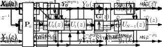
Figure 1: A two-channel multirate analysis/synthesis filter bank.

Figure 2: The polyphase-with-delay (PWD) filter bank representation.

1.1 Background and Relation to Other Work

Many structures for fast, customizable implementations of PR filter banks consist of decompositions of the transfer matrices $\mathbf{H}(z)$ and $\mathbf{G}(z)$ into cascades (matrix products) of simpler matrix building blocks. Examples include decompositions for particular classes such as paraunitary or linear phase filter banks TranQueirozNguyen:00:Linear-phase-perfect-reconstruction; GaoNguyenStrang:01:M-channel-PUFBs; OrainTranHellerNgu:01:paraunitary-linear-phase; GanMaNguyenEtal:02:on-completeness; OrainTranNgu:03:regular-LPFBs; GanMa:TCAS-II-04:simplified-lattice; GanMa:TSP-04:simplified-order-one; MakMuthRed:04:Eigenstructure-approach; XuMakur:09:Arbitrary-Length-LPPRFB and low-complexity structures like cosine-modulated filter banks Vaid93; StrNgu96; PainterSpanias:00:Perceptual-Coding; KhaTuanNgu:ICASSP07:SDP-Cos-Mod-FB; KhaTuanNguyen:09:Cos-Mod-FBs. The cascade structures studied in this paper are lifting factorizations Sweldens96; Sweldens:98:SIAM-lifting-scheme; DaubSwel98, which factor $\mathbf{H}(z)$ and $\mathbf{G}(z)$ into elementary (or “lifting”) matrices $\mathbf{S}(z)$ of the form

$$\mathbf{S}(z)=\begin{bmatrix}1&0\\ S(z)&1\vspace{-1pt}\end{bmatrix}\text{ or\ \ }\mathbf{S}(z)=\begin{bmatrix}1&S(z)\\ 0&1\vspace{-2pt}\end{bmatrix}.$$ (2)

Lifting figures prominently in image communication standards like the ISO/IEC JPEG 2000 image coding standards ISO_15444_1; ISO_15444_2; TaubMarc02; BrisQuirk03; AcharyaTsai:04:JPEG2000-Standard; Lee:05:J2K-Retrospective and CCSDS Recommendation 122.0 for Space Data System Standards CCSDS_122.0:2005; YehArmKielyEtal:AC-05:CCSDS-image-comp.

The lifting scheme of Daubechies and Sweldens DaubSwel98 factors unimodular polyphase matrices (matrices of determinant 1) using the Extended Euclidean Algorithm (EEA) MacLaneBirkhoff67; BachShallit:96:Algo-Number-Theory; Shoup:05:Comp-Number-Theory; GathenGerhard:13:Modern-Computer-Algebra for computing greatest common divisors (gcds) over the Laurent polynomials in $z$ and $z^{-1}$, denoted $\mathbb{C}[z,z^{-1}]$. This is a curious approach since the Laurent polynomials in question are always coprime! Their goal, however, was not to find gcds but rather to obtain computational byproducts of the EEA. The term “lifting” seems to originate with Sweldens Sweldens96, although the result now known as the Lifting Theorem had appeared earlier in the dissertation of Herley Herley93; VetterliHerley:92:Wavelets-filter-banks. The EEA was not used in Sweldens96, which uses lifting to synthesize high-order wavelets rather than for decomposing a given wavelet transform. The Euclidean Algorithm does appear in Daubechies, however, in the proof of Bezout’s Theorem for polynomials (Daub92, Theorem 6.1.1). Daubechies credits Y. Meyer (Daub92, Chapter 6, endnote 2) for suggesting the use of Bezout’s Theorem to factor trigonometric polynomials when constructing smooth wavelets, so Meyer deserves some credit for the closely related use of the Euclidean Algorithm in lifting factorization.

Lifting was anticipated by others, including Tolhuizen et al. TolHollKal:95:realiz-biorthog-M-D, who studied existence of elementary matrix decompositions for multivariate matrix polynomials. Cohn Cohn:66:structure-ring constructed an example of a $2\times 2$ bivariate matrix polynomial with no elementary matrix decompositions, but Suslin Suslin:77:structure-special subsequently proved that elementary matrix decompositions exist for all multivariate matrix polynomials of size $3\times 3$ or greater. A constructive proof using Gröbner bases was found by Park and Woodburn ParkWoodburn:95:algorithmic-proof. The univariate challenge is not the existence of elementary matrix decompositions; as noted in TolHollKal:95:realiz-biorthog-M-D, univariate polynomial (resp., Laurent polynomial) matrices can always be factored into elementary matrices using the polynomial (resp., Laurent polynomial) EEA. The univariate challenge is, instead, to define and systematically generate “good” lifting decompositions well-suited to a user’s application.

Since the appearance of DaubSwel98, some work on lifting has studied two-channel filter banks AdamsKossentini:00:Reversible-wavelet-transforms; MaslenAbbott:00:Automation-lifting-factorisation; ShuiBaoEtal:02:Two-channel-adaptive-biorthogonal; AdamsWard:03:Symmetric-extension-compatible; LiaoMandalEtal:04:Efficient-architectures-lifting-based but much has focused on $M>2$ channels Tran:02:M-channel-linear-phase; Tran:02:Rational-LPPRFBs; ChenAmaratun:03:M-channel-lifting-factorization; OrainTranNgu:03:regular-LPFBs; ShuiBao:04:M-band-biorthogonal-interpolating; ChenOrainAmara:05:Dyadic-based-factorizations; IwamuraTanakaIkehara:07:Efficient-Lifting; TanIkeNgu:08:LPFB-Lattice-Structure; SuzukiIkeharaNguyen:12:Generalized-Block-Lifting and related methods like linear predictive transform coding WengChenVaid:10:General-Triang-Decomp; WengVaid:12:GTD-Optimizing-PRFBs. The limitation of mathematical technique in DaubSwel98 (and in most of the literature since DaubSwel98) to linear algebra and the Euclidean Algorithm strikes the author as unduly restrictive. Herley’s dissertation Herley93; VetterliHerley:92:Wavelets-filter-banks noted a connection to Diophantine equations, but that idea was not followed up in subsequent papers, and the use of abstract algebra in filter bank theory has remained largely unexplored with only occasional exceptions FooteMirchandEtal:00:Wreath-Product-Group; MirchandFooteEtal:00:Wreath-Product-Group; FooteMirchandEtal:04:Two-Dimensional-Wreath-Product; Park:04:Symbolic-computation-signal; LebrunSelesnic:04:Grobner-bases-wavelet; DuBhosriFrazho:10:FB-commutant-lifting; HurParkZheng:14:Multi-D-Wavelet.

We shall focus on gaining a deeper understanding of the two-channel case, which has yielded significant applications to date such as digital communications coding and which informs our understanding of the more difficult $M$-channel case. The two-channel case has also proven amenable to nonlinear algebraic methods. After serving on the JPEG standards committee (ISO/IEC JTC1/SC29/WG1) the author developed a group-theoretic approach to lifting for two-channel unimodular linear phase FIR PR filter banks BrisWohl06; Bris:10:GLS-I; Bris:10b:GLS-II. It was shown that factoring linear phase filter banks using linear phase lifting filters produces factorizations that are unique within “universes” of factorizations that the author called group lifting structures. These uniqueness results were used Bris:13b:TIT to characterize the group of unimodular whole-sample symmetric (WS, or odd-length linear phase) filter banks up to isomorphism. It was also shown that the class of unimodular half-sample symmetric (HS, or even-length linear phase) filter banks, which is not a group, can nonetheless be partitioned into cosets of similar groups. An overview is given in Bris:13:FFT.

This work is the author’s response to Daubechies and Sweldens DaubSwel98, who sacrificed causality to exploit nonuniqueness of Laurent polynomial division. An FIR filter is causal if its transfer function is polynomial in $z^{-1}$. Converting noncausal unimodular factorizations into “equivalent” minimal causal realizations suitable for implementation is not straightforward, so sacrificing realizability is a big price to pay for mathematical options. It begs the question of just how many factorizations Laurent division creates; there appears to be no systematic way to enumerate “all possible” clever uses of Laurent division. It also highlights the lack of a definition in DaubSwel98 of what, exactly, makes an elementary matrix decomposition a lifting factorization. What is the difference between the “nice” (lifting) factorizations in DaubSwel98 and pathological factorizations like (Bris:10:GLS-I, Proposition 1 and Example 1) or (Bris:13b:TIT, Example 1)?

By taking an algebraic perspective we develop lifting from basic properties of linear Diophantine equations (LDEs) over polynomial rings. We show that much of lifting factorization, including the Lifting Theorem Herley93; VetterliHerley:92:Wavelets-filter-banks; Sweldens96, follows from basic factorization theory in commutative rings and does not involve polynomials per se. One is led naturally from abstract algebraic considerations to issues that really require polynomials and causality, such as degree inequalities and uniqueness results. This leads to a new lifting strategy, demonstrated by example in this paper and developed formally in work in progress, that we call the Causal Complementation Algorithm (CCA).

1.2 Degree-Reducing Causal Complements and Degree-Lifting Factorizations

Lifting factorization of a transfer matrix $\mathbf{H}(z)$ involves factoring off elementary matrices (2). E.g., left-factorization of an upper-triangular elementary matrix reduces row 0 (the top row) of $\mathbf{H}$; suppressing the $z$ for clarity,

$$\mathbf{H}(z)\stackrel{{\scriptstyle\mbox{\tiny{def}}}}{{=}}\begin{bmatrix}E_{0}&E_{1}\\ F_{0}&F_{1}\vspace{-2pt}\end{bmatrix}=\begin{bmatrix}1&S\\ 0&1\vspace{-2pt}\end{bmatrix}\begin{bmatrix}R_{0}&R_{1}\\ F_{0}&F_{1}\vspace{-2pt}\end{bmatrix}.$$ (3)

To get (3), pick a column index $j\in\{0,1\}$ and divide the pivot $F_{j}$ into $E_{j}$ using polynomial division to get $E_{j}=F_{j}S+R_{j}$, where remainder $R_{j}$ satisfies the degree-reducing condition $\deg(R_{j})<\deg(F_{j}).$ The corresponding remainder in column $j^{\prime}\stackrel{{\scriptstyle\mbox{\tiny{def}}}}{{=}}1-j$ of (3) for the same lifting filter (or quotient) $S$ is defined to be $R_{j^{\prime}}\stackrel{{\scriptstyle\mbox{\tiny{def}}}}{{=}}E_{j^{\prime}}-F_{j^{\prime}}S$, so that

$$(R_{0},R_{1})=(E_{0},E_{1})-S(F_{0},F_{1}),$$

a Gaussian elimination reduction of row 0. There are two such lifting factorizations depending on the column in which we perform the polynomial division. Analogous left-factorizations of lower-triangular elementary matrices correspond to Gaussian elimination reductions of row 1 in $\mathbf{H}$ while right-factorizations of elementary matrices correspond to column reductions.

Given a filter $H_{i}(z)$, $i\in\{0,1\}$, Herley and Vetterli Herley93; VetterliHerley:92:Wavelets-filter-banks call a second filter $H_{i^{\prime}}(z)$, where $i^{\prime}\stackrel{{\scriptstyle\mbox{\tiny{def}}}}{{=}}1-i$, a complementary filter if $\{H_{0}(z),H_{1}(z)\}$ is a PR filter bank. FIR filters $H_{0}$ and $H_{1}$ are complementary if and only if their polyphase components satisfy (1), motivating the following polyphase notion of complementary filters in the causal case (i.e., for polynomials in $z^{-1}$).

Definition 1

Let $F_{0},\,F_{1}$ be causal FIR filters satisfying $\gcd(F_{0},F_{1})=z^{-d}$, $d=\deg\gcd(F_{0},F_{1})$. Given constant $\hat{a}\neq 0$ and integer $\hat{d}\geq d$, an ordered pair of causal filters $(R_{0},R_{1})$ is a causal complement to $(F_{0},F_{1})$ for inhomogeneity $\hat{a}z^{-\hat{d}}$ if it satisfies the linear Diophantine polynomial equation

$$R_{0}(z)F_{1}(z)-R_{1}(z)F_{0}(z)=\hat{a}z^{-\hat{d}}.$$ (4)

We say a causal complement $(R_{0},R_{1})$ is degree-reducing in $F_{\ell},\,\ell\in\{0,1\}$, if

$$\deg(R_{\ell})<\deg(F_{\ell})-\deg\gcd(F_{0},F_{1}).$$ (5)

Figure 3: Standard causal lifting form for a FIR PR filter bank. In this example the initial lifting matrix, $\mathbf{U}_{0}(z)$, corresponding to the left-most lifting filter, $U_{0}(z)$, is lower-triangular, and the number of lifting steps, $N$, is odd.

Remarks. In the language of Definition 1, the CCA constructs factorizations of the form (3) by using polynomial division to compute degree-reducing causal complements $(R_{0},R_{1})$ for inhomogeneity $\hat{a}z^{-\hat{d}}=|\mathbf{H}(z)|$ without using the EEA. The reason for the correction term $\deg\gcd(F_{0},F_{1})$ in (5) is explained in Section LABEL:sec:Polynomial:SizeReducing following Definition LABEL:defn:SizeReducing; existence and uniqueness of degree-reducing causal complements are addressed by Theorem LABEL:thm:LDDRT.

In the course of factorization, the degree-reducing property (5) eventually drives one of the remainders $R_{i}$ to zero, causing factorization to terminate. The result can then be put into standard causal lifting form (cf. Figure 3),

$$\mathbf{H}(z)=\mbox{\rm diag}(\kappa_{0}z^{-\rho_{0}},\kappa_{1}z^{-\rho_{1}})\mathbf{U}_{\!N-1}(z)\boldsymbol{\Lambda}_{N-1}(z)\cdots\\ \cdots\mathbf{U}_{1}(z)\boldsymbol{\Lambda}_{1}(z)\mathbf{U}_{0}(z)\mbox{$\mathbf{P}_{\!0}$}\,\mbox{\rm diag}(z^{-c_{0}},z^{-c_{1}}).$$ (6)

The causal matrices $\mathbf{U}_{n}(z)$ in (6) are alternating upper- and lower-triangular lifting matrices (2) with causal lifting filters $U_{n}(z)$. The matrices $\boldsymbol{\Lambda}_{n}(z)$ are diagonal delay matrices; they have a single delay factor $z^{-m_{n}},$ $m_{n}\geq 0,$ in the upper channel, $\boldsymbol{\Lambda}_{n}(z)=\mbox{\rm diag}(z^{-m_{n}},1)$, or (resp.) the lower channel, $\mbox{\rm diag}(1,z^{-m_{n}})$, if and only if $\mathbf{U}_{n}(z)$ is upper-triangular (resp., lower-triangular). $\mathbf{P}_{\!0}$ is either the identity, $\mathbf{I}$, or the swap matrix,

$$\mathbf{J} \stackrel{{\scriptstyle\mbox{\tiny{def}}}}{{=}}\begin{bmatrix}0&1\\ 1&0\vspace{-1pt}\end{bmatrix},\quad\mathbf{J}^{-1}=\mathbf{J}.$$ (7)

Using the CCA, every causal FIR PR filter bank has a factorization (many, in fact) in standard causal lifting form. We shall see that the ability to factor off diagonal delay matrices $\boldsymbol{\Lambda}_{n}(z)$ is a major advantage the CCA holds over the causal version of the EEA lifting factorization method.

The ancient Euclidean Algorithm was a clever idea for recursively reducing the gcd of “large” arguments to the gcd of “smaller” arguments. The notion of degree-reducing solutions to LDEs over polynomial rings (Definition 1) captures the size-reducing aspect of the EEA without its misleading focus on gcds. Moreover, the degree-reducing notion applies to factorizations of arbitrary FIR PR filter banks whereas the polyphase order-increasing property employed in Bris:10:GLS-I; Bris:10b:GLS-II was found to be useful only for linear phase filter banks. A degree-reducing decomposition corresponds to a degree-increasing synthesis, so we use the neutral term degree-lifting to encompass both decomposition and synthesis. The author holds that this degree-lifting character of both the EEA and the CCA distinguishes lifting factorizations within the much bigger universe of elementary matrix decompositions, a distinction not made in DaubSwel98.

1.3 Overview of the Paper

Section 2 introduces LGT(5,3), the LeGall-Tabatabai 5-tap/3-tap piecewise-linear spline wavelet filter bank LeGallTabatabai:88:Subband-coding-digital; ISO_15444_1, and uses it to illustrate a connection between causality and uniqueness of lifting factorizations. Factorizations of LGT(5,3) made by the causal EEA and the Causal Complementation Algorithm are compared. It is shown that the CCA generates all of the causal lifting factorizations formed by the causal version of the EEA approach plus others not generated by it, generalizing the degree-lifting aspects of the EEA.

To understand the connection between causal lifting and uniqueness of factorizations, Section 3 defines linear Diophantine equations (LDEs) and reviews the commutative ring theory needed to characterize the solution sets of homogeneous LDEs (the Homogeneous LDE Theorem) and inhomogeneous LDEs (the Abstract Lifting Theorem). Necessary and sufficient conditions are given for existence (but not uniqueness) of solutions to inhomogeneous LDEs in principal ideal domains (the Abstract Bezout Theorem). Section LABEL:sec:LDE:Euclidean reviews the differences between polynomials and Laurent polynomials.

Degree-reducing causal complements are generalized in Definition LABEL:defn:SizeReducing to include LDEs over the Laurent polynomials. By Lemma LABEL:lem:LDE_uniqueness degree-reducing solutions to polynomial LDEs are unique thanks to a max-additive inequality, whose failure for the Laurent order explains why filters can have multiple Laurent-order-reducing complements. Existence and uniqueness of degree-reducing solutions (in either unknown) to polynomial LDEs are given by the Linear Diophantine Degree-Reduction Theorem (LDDRT), which provides necessary and sufficient conditions for the two solutions to agree.

Section LABEL:sec:LDE:Division uses the LDDRT to prove existence and uniqueness of quotients whose remainders satisfy degree-reducing inequalities and user-specified divisibility constraints (the Generalized Polynomial Division Theorem). This is specialized to the case of remainders divisible by monomials and given a constructive proof in the Slightly Generalized Division Theorem, yielding a Slightly Generalized Division Algorithm (SGDA, Algorithm LABEL:alg:SGDA).

Section LABEL:sec:CubicBSpline returns to the filter bank setting and presents a case study using CDF(7,5), a 7-tap/5-tap cubic B-spline wavelet filter bank DaubSwel98. It is shown that the causal EEA and CCA factorizations in column 1 are the same. To produce a causal version of a unimodular linear phase lifting factorization obtained by Daubechies and Sweldens (DaubSwel98, §7.8), we use the SGDA to factor off a diagonal delay matrix with the first CCA lifting step. This factorization is not produced by running the causal EEA in any row or column of CDF(7,5).

Section LABEL:sec:Conclusions summarizes the paper’s contributions.

2 Case Study: The LeGall-Tabatabai Filter Bank

We begin by contrasting the CCA and causal EEA approaches to factoring LGT(5,3), the 5-tap/3-tap LeGall-Tabatabai biorthogonal linear phase filter bank LeGallTabatabai:88:Subband-coding-digital, whose analog synthesis scaling function and mother wavelet generate piecewise-linear B-splines. JPEG 2000 Part 1 ISO_15444_1 specifies it via a unimodular lifting factorization of its noncausal whole-sample symmetric analysis filters

$$\begin{split}A_{0}(z)&=-z^{2}/8+z/4+3/4+z^{-1}/4-z^{-2}/8,\\ A_{1}(z)&=-z^{2}/2+z-1/2.\end{split}$$ (8)

The JPEG 2000 factorization of its unimodular polyphase-with-advance (PWA) matrix representation $\mathbf{A}(z)$ DaubSwel98; BrisWohl06 is its unique lifting factorization in the unimodular WS group of whole-sample symmetric transfer matrices (Bris:10:GLS-I, Definition 8), whose lifting cascades satisfy a polyphase order-increasing property,

$$\mathbf{A}(z) =\begin{bmatrix}\scriptstyle(-z+6-z^{-1})/8&\scriptstyle\;(1+z^{-1})/4\\ \scriptstyle-(z+1)/2&\scriptstyle 1\vspace{-1pt}\end{bmatrix}=\begin{bmatrix}\scriptstyle 1&\scriptstyle(1+z^{-1})/4\\ \scriptstyle 0&\scriptstyle 1\vspace{-1pt}\end{bmatrix}\begin{bmatrix}\scriptstyle 1&\scriptstyle 0\\ \scriptstyle-(z+1)/2&\scriptstyle 1\vspace{-1pt}\end{bmatrix}.$$ (9)

We will work instead with the causally normalized filters

$$\begin{split}H_{0}(z)&=(-1+2z^{-1}+6z^{-2}+2z^{-3}-z^{-4})/8,\\ H_{1}(z)&=(-1+2z^{-1}-z^{-2})/2\end{split}$$ (10)

and their causal polyphase-with-delay (PWD) matrix Vaid93; StrNgu96,

$$\mathbf{H}(z)=\begin{bmatrix}(-1+6z^{-1}-z^{-2})/8&\;(1+z^{-1})/4\\ -(1+z^{-1})/2&1\vspace{-1pt}\end{bmatrix}.$$ (11)

Laurent polynomials can have multiple reduced-order unimodular complements (shorter filters with which they form a unimodular filter bank). For instance, $A_{0}(z)$ also has the reduced-order nonlinear phase unimodular complement $A^{\prime}_{1}(z)=-7/2-z^{-1}+z^{-2}/2$, which happens to be causal. $A_{0}(z)$ and $A^{\prime}_{1}(z)$ have noncausal unimodular PWA matrix $\mathbf{A}^{\prime}(z)$,

$$\mathbf{A}^{\prime}(z) =\begin{bmatrix}(-z+6-z^{-1})/8&\;(1+z^{-1})/4\\ (-7+z^{-1})/2&-z^{-1}\vspace{-1pt}\end{bmatrix},$$

while $H_{0}(z)$ and $H^{\prime}_{1}(z)\stackrel{{\scriptstyle\mbox{\tiny{def}}}}{{=}}A^{\prime}_{1}(z)$ have causal PWD counterpart $\mathbf{H}^{\prime}(z)$,

$$\mathbf{H}^{\prime}(z) =\begin{bmatrix}(-1+6z^{-1}-z^{-2})/8&\;(1+z^{-1})/4\\ (-7+z^{-1})/2&-1\vspace{-1pt}\end{bmatrix}.$$

The determinants of $\mathbf{A}(z)$ and $\mathbf{A}^{\prime}(z)$ are both 1, but $|\mathbf{H}(z)|=z^{-1}$ and $|\mathbf{H}^{\prime}(z)|=1$ distinguish between the two reduced-degree causal complements of $H_{0}(z)$. Theorem LABEL:thm:LDDRT will imply that $H_{1}(z)$ and $H^{\prime}_{1}(z)$ are the unique reduced-degree causal complements to $H_{0}(z)$ for these determinants. This shows that the unimodular normalization employed by Daubechies and Sweldens DaubSwel98 is discarding useful information about filter banks. Using Theorem LABEL:thm:LDDRT and the connection between lifting factorization and degree-lifting causal complementation, the Diophantine perspective uncovers a connection between causality and uniqueness of lifting factorizations that allows the CCA to enumerate and generate all causal degree-lifting factorizations of a causal filter bank.

2.1 Causal Factorization via the Causal Extended Euclidean Algorithm

There are four possible factorizations based on running the causal EEA in either row or column of $\mathbf{H}(z)$. Our notation for the EEA is a compromise between several sources, including DaubSwel98, BachShallit:96:Algo-Number-Theory, Shoup:05:Comp-Number-Theory, and GathenGerhard:13:Modern-Computer-Algebra.

2.1.1 EEA in Column 0

Initialize remainders $r_{0}\stackrel{{\scriptstyle\mbox{\tiny{def}}}}{{=}}H_{00}(z)=(-1+6z^{-1}-z^{-2})/8$ and $r_{1}\stackrel{{\scriptstyle\mbox{\tiny{def}}}}{{=}}H_{10}(z)=-(1+z^{-1})/2$. Iterate using the polynomial division algorithm, $r_{0}=q_{0}r_{1}+r_{2}$,

$$q_{0}=(-7+z^{-1})/4,\;r_{2}=-1,\text{ and }\deg(r_{2})=0<\deg(r_{1})=1.$$ (12)

Define the matrix

$$\mathbf{M}_{0} \stackrel{{\scriptstyle\mbox{\tiny{def}}}}{{=}}\begin{bmatrix}q_{0}&1\\ 1&0\end{bmatrix},\text{ so that }\begin{pmatrix}r_{0}\\ r_{1}\end{pmatrix}=\mathbf{M}_{0}\begin{pmatrix}r_{1}\\ r_{2}\end{pmatrix}.$$ (13)

Remainder $r_{2}$ is invertible so the next division step yields

$$r_{3}=r_{1}-q_{1}r_{2}=0\mbox{ with }q_{1}=r_{1}/r_{2}=(1+z^{-1})/2,$$ (14)

where $\deg(r_{3})=\deg(0)\stackrel{{\scriptstyle\mbox{\tiny{def}}}}{{=}}-\infty<\deg(r_{2})$. Define

$$\mathbf{M}_{1}\stackrel{{\scriptstyle\mbox{\tiny{def}}}}{{=}}\begin{bmatrix}q_{1}&1\\ 1&0\end{bmatrix},\text{ so that }\begin{pmatrix}r_{1}\\ r_{2}\end{pmatrix}=\mathbf{M}_{1}\begin{pmatrix}r_{2}\\ r_{3}\end{pmatrix}.$$ (15)

Iteration terminates since $r_{3}=0$, and (13) and (15) imply

$$\begin{pmatrix}r_{0}\\ r_{1}\end{pmatrix}=\mathbf{M}_{0}\mathbf{M}_{1}\begin{pmatrix}r_{2}\\ 0\end{pmatrix}.$$ (16)

Put two swap matrices between $\mathbf{M}_{0}$ and $\mathbf{M}_{1}$ to get lifting matrices $\mathbf{S}_{0}$ and $\mathbf{S}_{1}$,

$$\mathbf{M}_{0}\mathbf{M}_{1} =(\mathbf{M}_{0}\mathbf{J})(\mathbf{J}\mathbf{M}_{1})=\begin{bmatrix}1&q_{0}\\ 0&1\end{bmatrix}\begin{bmatrix}1&0\\ q_{1}&1\end{bmatrix}=\mathbf{S}_{0}\mathbf{S}_{1}.$$

As in the unimodular approach DaubSwel98, form an augmentation matrix $\mathbf{H}^{\prime}(z)$ by augmenting (16) with causal filters $a_{0}$ and $a_{1}$ determined by the condition

$$\mathbf{H}^{\prime}(z) \stackrel{{\scriptstyle\mbox{\tiny{def}}}}{{=}}\begin{bmatrix}r_{0}&a_{0}\\ r_{1}&a_{1}\vspace{1pt}\end{bmatrix}=\mathbf{S}_{0}\mathbf{S}_{1}\begin{bmatrix}r_{2}&0\\ 0&|\mathbf{H}(z)|/r_{2}\end{bmatrix}$$

$$=\begin{bmatrix}1&(-7+z^{-1})/4\\ 0&1\vspace{-1pt}\end{bmatrix}\begin{bmatrix}1&0\\ (1+z^{-1})/2&1\vspace{-1pt}\end{bmatrix}\begin{bmatrix}-1&0\\ 0&-z^{-1}\vspace{-1pt}\end{bmatrix}$$ (17)

$$=\begin{bmatrix}(-1+6z^{-1}-z^{-2})/8&\;(7z^{-1}-z^{-2})/4\\ -(1+z^{-1})/2&-z^{-1}\vspace{-1pt}\end{bmatrix}.$$

$|\mathbf{H}^{\prime}(z)|=|\mathbf{H}(z)|$ by (2.1.1) and the matrices agree in column 0, so the Lifting Theorem Herley93; VetterliHerley:92:Wavelets-filter-banks; Sweldens96 (or Corollary 1 below) says that $\mathbf{H}(z)$ can be lifted from $\mathbf{H}^{\prime}(z)$ by a causal lifting update to column 1, $\mathbf{H}(z)=\mathbf{H^{\prime}}(z)\mathbf{S}(z)$,

$$\mathbf{H}(z) =\begin{bmatrix}H_{00}&H_{01}\\ H_{10}&H_{11}\vspace{-1pt}\end{bmatrix}=\begin{bmatrix}r_{0}&a_{0}\\ r_{1}&a_{1}\vspace{1pt}\end{bmatrix}\begin{bmatrix}1&S\\ 0&1\vspace{-1pt}\end{bmatrix}\text{\ iff\ }\left\{\begin{array}[]{l}H_{01}=r_{0}S+a_{0}\\ H_{11}=r_{1}S+a_{1}\,.\end{array}\right.$$ (20)

Compute $H_{01}-a_{0}=(1-6z^{-1}+z^{-2})/4=-2r_{0}$, so $S=-2$. The resulting factorization in standard causal lifting form (6) based on (2.1.1)–(20) is

$$\mathbf{H}(z) =-\begin{bmatrix}1&(-7+z^{-1})/4\\ 0&1\end{bmatrix}\begin{bmatrix}1&0\\ (1+z^{-1})/2&1\end{bmatrix}\begin{bmatrix}1&0\\ 0&z^{-1}\end{bmatrix}\begin{bmatrix}1&-2\\ 0&1\end{bmatrix}.$$ (21)

2.1.2 EEA in Column 1

Initialize $r_{0}\stackrel{{\scriptstyle\mbox{\tiny{def}}}}{{=}}H_{01}(z)=(1+z^{-1})/4$ and $r_{1}\stackrel{{\scriptstyle\mbox{\tiny{def}}}}{{=}}H_{11}(z)=1$. Polynomial division yields $q_{0}=r_{0}/r_{1}=(1+z^{-1})/4$, and $r_{2}=0$ since $r_{1}$ is invertible so

$$\begin{pmatrix}r_{0}\\ r_{1}\end{pmatrix}=\mathbf{M}_{0}\begin{pmatrix}r_{1}\\ 0\end{pmatrix}\text{ with }\mathbf{M}_{0}\stackrel{{\scriptstyle\mbox{\tiny{def}}}}{{=}}\begin{bmatrix}q_{0}&1\\ 1&0\end{bmatrix},\;|\mathbf{M}_{0}|=-1.$$ (22)

Augment (22) in column 0 with causal filters $a_{0}$ and $a_{1}$ defined by

$$\mathbf{H}^{\prime}(z) \stackrel{{\scriptstyle\mbox{\tiny{def}}}}{{=}}\begin{bmatrix}a_{0}&r_{0}\\ a_{1}&r_{1}\end{bmatrix}=\mathbf{M}_{0}\begin{bmatrix}0&r_{1}\\ |\mathbf{H}|/r_{1}&0\end{bmatrix}=\mathbf{M}_{0}\,\mathbf{J}^{2}\begin{bmatrix}0&r_{1}\\ |\mathbf{H}|/r_{1}&0\end{bmatrix}$$ (23)

$$=\begin{bmatrix}1\;&(1+z^{-1})/4\\ 0&1\vspace{-1pt}\end{bmatrix}\begin{bmatrix}z^{-1}&0\\ 0&1\end{bmatrix}.$$

$|\mathbf{H}^{\prime}(z)|=|\mathbf{H}(z)|$ and the matrices agree in column 1 so $\mathbf{H}(z)$ can be lifted from the augmentation matrix $\mathbf{H}^{\prime}(z)$ by a causal lifting update to column 0,

$$\mathbf{H}(z) =\begin{bmatrix}H_{00}&H_{01}\\ H_{10}&H_{11}\vspace{-1pt}\end{bmatrix}=\begin{bmatrix}a_{0}&r_{0}\\ a_{1}&r_{1}\vspace{1pt}\end{bmatrix}\begin{bmatrix}1&0\\ S&1\vspace{-1pt}\end{bmatrix}\text{\ iff\ }\left\{\begin{array}[]{l}H_{00}=r_{0}S+a_{0}\\ H_{10}=r_{1}S+a_{1}\,.\end{array}\right.$$ (26)

$H_{00}-a_{0}=-(1+2z^{-1}+z^{-2})/8=r_{0}S$ for $S(z)=-(1+z^{-1})/2$ so by (26)

$$\mathbf{H}(z) =\begin{bmatrix}1&(1+z^{-1})/4\\ 0&1\vspace{-1pt}\end{bmatrix}\begin{bmatrix}z^{-1}&0\\ 0&1\vspace{-1pt}\end{bmatrix}\begin{bmatrix}1&0\\ -(1+z^{-1})/2&1\vspace{-1pt}\end{bmatrix}.$$ (27)

Remarks. This is a causal analogue for the noncausal linear phase lifting (9) of the unimodular LGT(5,3) analysis bank; its causal linear phase lifting filters differ from the corresponding lifting filters in (9) by at most delays.

2.1.3 EEA in Row 0

Initialize $r_{0}\stackrel{{\scriptstyle\mbox{\tiny{def}}}}{{=}}H_{00}(z)=(-1+6z^{-1}-z^{-2})/8$ and $r_{1}\stackrel{{\scriptstyle\mbox{\tiny{def}}}}{{=}}H_{01}(z)=(1+z^{-1})/4$. Division yields $r_{2}=r_{0}-r_{1}q_{0}=-1$ where $q_{0}=(7-z^{-1})/2$ and

$$(r_{0},\,r_{1})=(r_{1},\,r_{2})\,\mathbf{M}_{0},\text{ with }\mathbf{M}_{0}\stackrel{{\scriptstyle\mbox{\tiny{def}}}}{{=}}\begin{bmatrix}q_{0}&1\\ 1&0\end{bmatrix}.$$ (28)

Since $r_{2}=-1$ is invertible, we get $q_{1}=r_{1}/r_{2}=-(1+z^{-1})/4$, $r_{3}=0$, and

$$(r_{1},\,r_{2})=(r_{2},\,0)\,\mathbf{M}_{1},\text{ with }\mathbf{M}_{1}\stackrel{{\scriptstyle\mbox{\tiny{def}}}}{{=}}\begin{bmatrix}q_{1}&1\\ 1&0\end{bmatrix}.$$ (29)

Combine (28) and (29) and define $\mathbf{S}_{0}\stackrel{{\scriptstyle\mbox{\tiny{def}}}}{{=}}\mathbf{J}\mathbf{M}_{0},\;\mathbf{S}_{1}\stackrel{{\scriptstyle\mbox{\tiny{def}}}}{{=}}\mathbf{M}_{1}\mathbf{J}$ to express the top row as $(r_{0},\,r_{1})=(r_{2},\,0)\,\mathbf{S}_{1}\mathbf{S}_{0}.$ Augment with filters $a_{0}$ and $a_{1}$,

$$\mathbf{H}^{\prime}(z) \stackrel{{\scriptstyle\mbox{\tiny{def}}}}{{=}}\begin{bmatrix}r_{0}&r_{1}\\ a_{0}&a_{1}\end{bmatrix}=\begin{bmatrix}r_{2}&0\\ 0&\;|\mathbf{H}|/r_{2}\end{bmatrix}\mathbf{S}_{1}\mathbf{S}_{0}=\begin{bmatrix}\scriptstyle(-1+6z^{-1}-z^{-2})/8&\scriptstyle\;(1+z^{-1})/4\\ \scriptstyle(-7z^{-1}+z^{-2})/2&\scriptstyle-z^{-1}\vspace{-1pt}\end{bmatrix}.$$

$\mathbf{H}$ can be lifted from augmentation matrix $\mathbf{H}^{\prime}$ by updating row 1, $\mathbf{H}=\mathbf{S}\mathbf{H}^{\prime}$,

$$\begin{bmatrix}H_{00}&H_{01}\\ H_{10}&H_{11}\vspace{-1pt}\end{bmatrix} =\begin{bmatrix}1&0\\ S&1\vspace{-1pt}\end{bmatrix}\begin{bmatrix}r_{0}&r_{1}\\ a_{0}&a_{1}\vspace{1pt}\end{bmatrix}\text{\ iff\ }\left\{\begin{array}[]{l}H_{10}=r_{0}S+a_{0}\\ H_{11}=r_{1}S+a_{1}.\vspace{-1pt}\end{array}\right.$$

This implies $S(z)=4$, and the causal lifting factorization is

$$\mathbf{H}(z) =-\begin{bmatrix}1&0\\ 4&1\end{bmatrix}\begin{bmatrix}1&0\\ 0&z^{-1}\end{bmatrix}\begin{bmatrix}1&-(1+z^{-1})/4\\ 0&1\end{bmatrix}\begin{bmatrix}1&0\\ (7-z^{-1})/2&1\end{bmatrix}.$$ (30)

2.1.4 EEA in Row 1

This yields the causal linear phase lifting factorization (27).

2.2 Causal Factorization via the Causal Complementation Algorithm

We begin by using the CCA to reproduce all of the EEA factorizations.

2.2.1 CCA With Division in Column 0

Initialize quotient matrix $\mathbf{Q}_{0}(z)\stackrel{{\scriptstyle\mbox{\tiny{def}}}}{{=}}\mathbf{H}(z)$ and find an initial lifting of the form

$$\mathbf{Q}_{0}(z)=\begin{bmatrix}\scriptstyle(-1+6z^{-1}-z^{-2})/8&\scriptstyle\;(1+z^{-1})/4\\ \scriptstyle-(1+z^{-1})/2&\scriptstyle 1\vspace{-1pt}\end{bmatrix}=\begin{bmatrix}\scriptstyle E_{0}&\scriptstyle E_{1}\\ \scriptstyle F_{0}&\scriptstyle F_{1}\vspace{-1pt}\end{bmatrix}=\begin{bmatrix}\scriptstyle 1&\scriptstyle S\\ \scriptstyle 0&\scriptstyle 1\vspace{-1pt}\end{bmatrix}\begin{bmatrix}\scriptstyle R_{0}&\scriptstyle R_{1}\\ \scriptstyle F_{0}&\scriptstyle F_{1}\vspace{-1pt}\end{bmatrix}.$$ (31)

Set $E_{0}\leftarrow H_{00}$, $F_{0}\leftarrow H_{10}$, and divide $F_{0}$ into $E_{0}$ to get $E_{0}=F_{0}S+R_{0}$ with

$$S(z)=(-7+z^{-1})/4\text{ and }R_{0}(z)=-1,\text{ as in the EEA~{}\eqref{r2}.}$$ (32)

Set $R_{1}\leftarrow E_{1}-F_{1}S=2$ to get a row reduction, $(R_{0},R_{1})=(E_{0},E_{1})-S(F_{0},F_{1})$.

$R_{0}$ and $R_{1}$ are coprime, so the first lifting step (31) is

$$\mathbf{Q}_{0}(z) =\begin{bmatrix}1&(-7+z^{-1})/4\\ 0&1\vspace{-1pt}\end{bmatrix}\begin{bmatrix}-1&2\\ -(1+z^{-1})/2&\,1\vspace{-1pt}\end{bmatrix}=\mathbf{V}_{0}(z)\mathbf{Q}_{1}(z).$$ (33)

Reset $E_{j}\leftarrow F_{j}$ and $F_{j}\leftarrow R_{j}$ in $\mathbf{Q}_{1}(z)$ and divide again in column 0 to get

$$\mathbf{Q}_{1}(z)=\begin{bmatrix}-1&2\\ -(1+z^{-1})/2&1\vspace{-1pt}\end{bmatrix}=\begin{bmatrix}F_{0}&F_{1}\\ E_{0}&E_{1}\vspace{-1pt}\end{bmatrix}=\begin{bmatrix}1&0\\ S&1\vspace{-2pt}\end{bmatrix}\begin{bmatrix}F_{0}&F_{1}\\ R_{0}&R_{1}\vspace{-1pt}\end{bmatrix}.$$ (34)

Dividing $F_{0}=-1$ into $E_{0}=-(1+z^{-1})/2$ as in (14) gives $E_{0}=F_{0}S+R_{0}$,

$$S(z)=(1+z^{-1})/2\text{ and }R_{0}=0,\;\deg(R_{0})\stackrel{{\scriptstyle\mbox{\tiny{def}}}}{{=}}-\infty<\deg(F_{0}).$$ (35)

Set $R_{1}\leftarrow E_{1}-F_{1}S=-z^{-1}$; $\gcd(R_{0},R_{1})=z^{-1}$ so factor it out of $\mathbf{Q}_{2}(z)$,

$$\mathbf{Q}_{1}(z) =\begin{bmatrix}\scriptstyle 1&\scriptstyle 0\\ \scriptstyle(1+z^{-1})/2&\scriptstyle\,1\vspace{-1pt}\end{bmatrix}\begin{bmatrix}\scriptstyle-1&\scriptstyle 2\\ \scriptstyle 0&\scriptstyle-z^{-1}\vspace{-1pt}\end{bmatrix}=\begin{bmatrix}\scriptstyle 1&\scriptstyle 0\\ \scriptstyle(1+z^{-1})/2&\scriptstyle\,1\vspace{-1pt}\end{bmatrix}\begin{bmatrix}\scriptstyle 1&\scriptstyle 0\\ \scriptstyle 0&\scriptstyle z^{-1}\vspace{-1pt}\end{bmatrix}\begin{bmatrix}\scriptstyle-1&\scriptstyle 2\\ \scriptstyle 0&\scriptstyle-1\vspace{-1pt}\end{bmatrix}$$ (36)

$$=\mathbf{V}_{1}(z)\boldsymbol{\Delta}_{1}(z)\mathbf{Q}_{2}(z),\text{ where }\boldsymbol{\Delta}_{1}(z)=\mbox{\rm diag}(1,z^{-1}).$$

Combining (33) and (36) and dividing $\mathbf{Q}_{2}(z)$ by $-1$ to get a proper lifting step yields the same factorization (21) obtained using the EEA in column 0,

$$\mathbf{H}(z) =-\begin{bmatrix}1&(-7+z^{-1})/4\\ 0&1\end{bmatrix}\begin{bmatrix}1&0\\ (1+z^{-1})/2&1\end{bmatrix}\begin{bmatrix}1&0\\ 0&z^{-1}\end{bmatrix}\begin{bmatrix}1&-2\\ 0&1\end{bmatrix}.$$ (37)

2.2.2 CCA With Division in Column 1

Initialize $E_{1}\leftarrow H_{01}$ and $F_{1}\leftarrow H_{11}$. Divide $F_{1}$ into $E_{1}$ in (31) to get $E_{1}=F_{1}S+R_{1}$ where $S=(1+z^{-1})/4$ and $R_{1}=0.$ Set $R_{0}\leftarrow E_{0}-F_{0}S=z^{-1}$; factoring out $\gcd(R_{0},R_{1})=z^{-1}$ yields the lifting (27) obtained by the EEA,

$$\mathbf{H}(z)=\begin{bmatrix}1&(1+z^{-1})/4\\ 0&1\vspace{-1pt}\end{bmatrix}\begin{bmatrix}z^{-1}&0\\ 0&1\vspace{-1pt}\end{bmatrix}\begin{bmatrix}1&0\\ -(1+z^{-1})/2&\,1\vspace{-1pt}\end{bmatrix}.$$ (38)

2.2.3 CCA With Division in Row 0

Initialize $E_{0}\leftarrow H_{00}$ and $F_{0}\leftarrow H_{01}$ and divide $F_{0}$ into $E_{0}$ to get

$$\mathbf{Q}_{0}(z)=\begin{bmatrix}E_{0}&F_{0}\\ E_{1}&F_{1}\vspace{-1pt}\end{bmatrix}=\begin{bmatrix}R_{0}&F_{0}\\ R_{1}&F_{1}\vspace{-1pt}\end{bmatrix}\begin{bmatrix}1&0\\ S&1\vspace{-1pt}\end{bmatrix},\;S=(7-z^{-1})/2,\;R_{0}=-1.$$ (39)

Set $R_{1}\leftarrow E_{1}-F_{1}S=-4$. The first factorization step is

$$\mathbf{Q}_{0}(z) =\mathbf{Q}_{1}(z)\mathbf{V}_{0}(z)=\begin{bmatrix}-1&(1+z^{-1})/4\\ -4&\,1\vspace{-1pt}\end{bmatrix}\begin{bmatrix}1&0\\ (7-z^{-1})/2&\,1\vspace{-1pt}\end{bmatrix}.$$ (40)

Reset the labels $E_{j}\leftarrow F_{j}$ and $F_{j}\leftarrow R_{j}$ in $\mathbf{Q}_{1}(z)$, so that

$$\mathbf{Q}_{1}(z)=\begin{bmatrix}-1&(1+z^{-1})/4\\ -4&\,1\vspace{-1pt}\end{bmatrix}=\begin{bmatrix}F_{0}&E_{0}\\ F_{1}&E_{1}\vspace{-1pt}\end{bmatrix}.$$ (41)

Divide $F_{0}=-1$ into $E_{0}=(1+z^{-1})/4$,

$$E_{0} =F_{0}S+R_{0},\;S=-(1+z^{-1})/4,\text{ and }R_{0}=0.$$ (42)

The first two division steps (39) and (42) are identical to the first two steps in the row 0 EEA calculation, (28) and (29). Set $R_{1}\leftarrow E_{1}-F_{1}S=-z^{-1}$,

$$\mathbf{Q}_{1}(z)=\begin{bmatrix}F_{0}&R_{0}\\ F_{1}&R_{1}\vspace{-1pt}\end{bmatrix}\begin{bmatrix}1&S\\ 0&1\vspace{-1pt}\end{bmatrix}=\begin{bmatrix}-1&0\\ -4&-z^{-1}\vspace{-1pt}\end{bmatrix}\begin{bmatrix}1&\,-(1+z^{-1})/4\\ 0&1\vspace{-1pt}\end{bmatrix}.$$

Factor out $\gcd(R_{0},R_{1})=z^{-1}$; the resulting factorization agrees with (30),

$$\mathbf{H}(z) =-\begin{bmatrix}1&0\\ 4&1\end{bmatrix}\begin{bmatrix}1&0\\ 0&z^{-1}\end{bmatrix}\begin{bmatrix}1&-(1+z^{-1})/4\\ 0&1\end{bmatrix}\begin{bmatrix}1&0\\ (7-z^{-1})/2&1\end{bmatrix}.$$ (43)

2.2.4 CCA With Division in Row 1

The factorization is identical to the linear phase factorization (27), (38).

2.3 Other Degree-Lifting Factorizations via the CCA

It is convenient to have two algebraic tools for manipulating lifting cascades.

Definition 2 (cf. Bris:10:GLS-I, eq. (27))

Let $\mathbf{D}_{\kappa_{0},\kappa_{1}}\stackrel{{\scriptstyle\mbox{\tiny{def}}}}{{=}}\mbox{\rm diag}(\kappa_{0},\kappa_{1})$; $\kappa_{0},\kappa_{1}\neq 0$. The diagonal intertwining automorphism $\gamma_{\kappa_{0},\kappa_{1}}$ for matrices $\mathbf{A}$ is the matrix automorphism $\gamma_{\kappa_{0},\kappa_{1}}\mathbf{A}\stackrel{{\scriptstyle\mbox{\tiny{def}}}}{{=}}\mathbf{D}_{\kappa_{0},\kappa_{1}}\mathbf{A}\,\mathbf{D}^{-1}_{\kappa_{0},\kappa_{1}}$, which satisfies

$$\gamma_{\kappa_{0},\kappa_{1}}\!\begin{bmatrix}a&b\\ c&d\vspace{-2pt}\end{bmatrix} \stackrel{{\scriptstyle\mbox{\tiny{def}}}}{{=}}\begin{bmatrix}\kappa_{0}&0\\ 0&\kappa_{1}\end{bmatrix}\begin{bmatrix}a&b\\ c&d\vspace{-2pt}\end{bmatrix}\begin{bmatrix}\kappa_{0}^{-1\rule{0.0pt}{6.0pt}}&0\\ 0&\kappa_{1}^{-1}\end{bmatrix}=\begin{bmatrix}a&\kappa_{0}\kappa_{1}^{-1\rule{0.0pt}{6.0pt}}b\\ \kappa_{0}^{-1}\kappa_{1}c&d\end{bmatrix},$$ (44)

$$\mathbf{D}_{\kappa_{0},\kappa_{1}}\mathbf{A} =(\gamma_{\kappa_{0},\kappa_{1}}\mathbf{A})\mathbf{D}_{\kappa_{0},\kappa_{1}}\mbox{ and }\mathbf{A}\,\mathbf{D}_{\kappa_{0},\kappa_{1}}=\mathbf{D}_{\kappa_{0},\kappa_{1}}\,\gamma^{-1}_{\kappa_{0},\kappa_{1}}\mathbf{A}.$$ (45)

Definition 3

The double transpose automorphism is $\mathbf{A}^{\!\raisebox{1.0pt}{$\scriptstyle{\dagger}\!{\dagger}$}}\stackrel{{\scriptstyle\mbox{\tiny{def}}}}{{=}}\mathbf{J}\mathbf{A}\mathbf{J}$, for which

$$\begin{bmatrix}a&b\\ c&d\vspace{-2pt}\end{bmatrix}^{\raisebox{1.0pt}{$\scriptstyle{\dagger}\!{\dagger}$}} \stackrel{{\scriptstyle\mbox{\tiny{def}}}}{{=}}\begin{bmatrix}0&1\\ 1&0\vspace{-2pt}\end{bmatrix}\begin{bmatrix}a&b\\ c&d\vspace{-2pt}\end{bmatrix}\begin{bmatrix}0&1\\ 1&0\vspace{-2pt}\end{bmatrix}=\begin{bmatrix}d&c\\ b&a\vspace{-2pt}\end{bmatrix},$$ (46)

$$\mathbf{J}\mathbf{A} =\mathbf{A}^{\!\raisebox{1.0pt}{$\scriptstyle{\dagger}\!{\dagger}$}}\mathbf{J}\mbox{ and }\mathbf{A}\mathbf{J}=\mathbf{J}\mathbf{A}^{\!\raisebox{1.0pt}{$\scriptstyle{\dagger}\!{\dagger}$}}.$$ (47)

2.3.1 Switching Between Rows

We now construct CCA factorizations that are different from those obtained using the EEA by exploiting options that have no obvious EEA analogues. Consider (40), $\mathbf{Q}_{0}(z)\stackrel{{\scriptstyle\mbox{\tiny{def}}}}{{=}}\mathbf{H}(z)=\mathbf{Q}_{1}(z)\mathbf{V}_{0}(z)$, obtained by dividing in row 0. In Section 2.2.3 we factored $\mathbf{Q}_{1}(z)$ by dividing $F_{0}=-1$ into $E_{0}=(1+z^{-1})/4$ in (41). We are not obliged to continue dividing in row 0, however. Since

$$\deg|\mathbf{Q}_{1}(z)|=1>\deg(F_{0})+\deg(F_{1})=0,$$

Theorem LABEL:thm:LDDRT (below) implies that division in row 1 will produce a different lifting step than (42). Therefore, divide $F_{1}$ into $E_{1}$ in $\mathbf{Q}_{1}(z)$ to get $E_{1}=F_{1}S+R_{1}$, where $S=-1/4$ and $R_{1}=0$. Set $R_{0}\leftarrow E_{0}-F_{0}S=z^{-1}/4$ and factor $\gcd(R_{0},R_{1})=z^{-1}$ out of column 1 of the quotient matrix,

$$\mathbf{Q}_{1}(z) =\begin{bmatrix}F_{0}&R_{0}\\ F_{1}&R_{1}\vspace{-1pt}\end{bmatrix}\begin{bmatrix}1&S\\ 0&1\vspace{-1pt}\end{bmatrix}=\begin{bmatrix}-1&z^{-1}/4\\ -4&0\vspace{-1pt}\end{bmatrix}\begin{bmatrix}1&\,-1/4\\ 0&1\vspace{-1pt}\end{bmatrix}=\begin{bmatrix}-1&1/4\\ -4&0\vspace{-1pt}\end{bmatrix}\begin{bmatrix}1&0\\ 0&z^{-1}\vspace{-1pt}\end{bmatrix}\begin{bmatrix}1&\,-1/4\\ 0&1\vspace{-1pt}\end{bmatrix}$$

$$=\mathbf{Q}_{2}(z)\boldsymbol{\Delta}_{1}(z)\mathbf{V}_{1}(z),\text{ where }\boldsymbol{\Delta}_{1}(z)=\mbox{\rm diag}(1,z^{-1}).$$

$\mathbf{Q}_{2}(z)$ factors into a diagonal gain matrix, a lifting step, and a swap matrix,

$$\mathbf{Q}_{2}(z) =\begin{bmatrix}-1&1/4\\ -4&0\vspace{-1pt}\end{bmatrix}=\begin{bmatrix}1/4&0\\ 0&-4\vspace{-1pt}\end{bmatrix}\begin{bmatrix}1&-4\\ 0&1\vspace{-1pt}\end{bmatrix}\begin{bmatrix}0&1\\ 1&0\end{bmatrix}=\mbox{\rm diag}(1/4,-4)\mathbf{V}_{2}(z)\,\mathbf{J}.$$

Include the other matrices to get a causal lifting factorization (2.3.1) that is different from those obtained using the EEA in Section 2.1.

$$\mathbf{H}(z) =\mbox{\rm diag}(1/4,-4)\mathbf{V}_{2}(z)\,\mathbf{J}\,\boldsymbol{\Delta}_{1}(z)\mathbf{V}_{1}(z)\mathbf{V}_{0}(z)$$

$$=\mbox{\rm diag}(1/4,-4)\mathbf{V}_{2}(z)\boldsymbol{\Delta}_{1}^{\!\raisebox{1.0pt}{$\scriptstyle{\dagger}\!{\dagger}$}}(z)\mathbf{V}_{1}^{\!\raisebox{1.0pt}{$\scriptstyle{\dagger}\!{\dagger}$}}(z)\mathbf{V}_{0}^{\!\raisebox{1.0pt}{$\scriptstyle{\dagger}\!{\dagger}$}}(z)\,\mathbf{J}\text{\ \ by~{}\eqref{dbl_transpose}}$$

$$=\begin{bmatrix}\scriptstyle 1/4&\scriptstyle 0\\ \scriptstyle 0&\scriptstyle-4\end{bmatrix}\begin{bmatrix}\scriptstyle 1&\scriptstyle-4\\ \scriptstyle 0&\scriptstyle 1\end{bmatrix}\begin{bmatrix}\scriptstyle z^{-1}&\scriptstyle 0\\ \scriptstyle 0&\scriptstyle 1\end{bmatrix}\begin{bmatrix}\scriptstyle 1&\scriptstyle 0\\ \scriptstyle-1/4&\scriptstyle 1\end{bmatrix}\begin{bmatrix}\scriptstyle 1&\scriptstyle(7-z^{-1})/2\\ \scriptstyle 0&\scriptstyle 1\end{bmatrix}\begin{bmatrix}\scriptstyle 0&\scriptstyle 1\\ \scriptstyle 1&\scriptstyle 0\end{bmatrix}.$$ (48)

2.3.2 Switching Between Columns

Consider (33), $\mathbf{Q}_{0}(z)=\mathbf{V}_{0}(z)\mathbf{Q}_{1}(z)$, the initial lifting step obtained by dividing in column 0. In (34) we see that the first quotient $\mathbf{Q}_{1}(z)$ satisfies $\deg|\mathbf{Q}_{1}(z)|=1>\deg(F_{0})+\deg(F_{1})=0$ so Theorem LABEL:thm:LDDRT implies that division in column 1 of $\mathbf{Q}_{1}(z)$ yields a different lifting step than (35). Division in column 1 yields $S=E_{1}/F_{1}=1/2$, $R_{1}=0$, and $R_{0}\leftarrow E_{0}-F_{0}S=-z^{-1}/2$ so

$$\mathbf{Q}_{1}(z) =\begin{bmatrix}-1&2\\ -(1+z^{-1})/2&1\vspace{-1pt}\end{bmatrix}=\begin{bmatrix}1&0\\ S&1\vspace{-1pt}\end{bmatrix}\begin{bmatrix}F_{0}&F_{1}\\ R_{0}&R_{1}\vspace{-1pt}\end{bmatrix}=\begin{bmatrix}1&0\\ 1/2&1\vspace{-1pt}\end{bmatrix}\begin{bmatrix}1&0\\ 0&z^{-1}\vspace{-1pt}\end{bmatrix}\begin{bmatrix}-1&2\\ -1/2&0\vspace{-1pt}\end{bmatrix}$$

$$=\mathbf{V}_{1}(z)\boldsymbol{\Delta}_{1}(z)\mathbf{Q}_{2}(z).$$

$\mathbf{Q}_{2}(z)$ can be factored into a gain matrix, a lifting step, and a swap matrix,

$$\mathbf{Q}_{2}(z)=\begin{bmatrix}-1&2\\ -1/2&0\vspace{-1pt}\end{bmatrix}=\begin{bmatrix}2&0\\ 0&-1/2\vspace{-1pt}\end{bmatrix}\begin{bmatrix}1&-1/2\\ 0&1\vspace{-1pt}\end{bmatrix}\begin{bmatrix}0&1\\ 1&0\vspace{-1pt}\end{bmatrix}=\mbox{\rm diag}(2,-1/2)\mathbf{V}_{2}(z)\,\mathbf{J}.$$

The complete lifting factorization for $\mathbf{H}(z)$, which differs from (2.3.1) and from the EEA factorizations in Section 2.1, is

$$\mathbf{H}(z) =\mathbf{V}_{0}(z)\mathbf{V}_{1}(z)\boldsymbol{\Delta}_{1}(z)\,\mbox{\rm diag}(2,-1/2)\mathbf{V}_{2}(z)\,\mathbf{J}$$

$$=\mbox{\rm diag}(2,-1/2)\bigl{(}\gamma^{-1}_{\scriptscriptstyle 2,-1/2}\mathbf{V}_{0}(z)\bigr{)}\bigl{(}\gamma^{-1}_{\scriptscriptstyle 2,-1/2}\mathbf{V}_{1}(z)\bigr{)}\boldsymbol{\Delta}_{1}(z)\,\mathbf{V}_{2}(z)\,\mathbf{J}\text{ by~{}\eqref{symbolic_DIF},}$$

$$=\begin{bmatrix}\scriptstyle 2&\scriptstyle 0\\ \scriptstyle 0&\scriptstyle-1/2\end{bmatrix}\begin{bmatrix}\scriptstyle 1&\scriptstyle(7-z^{-1})/16\\ \scriptstyle 0&\scriptstyle 1\end{bmatrix}\begin{bmatrix}\scriptstyle 1&\scriptstyle 0\\ \scriptstyle-2&\scriptstyle 1\end{bmatrix}\begin{bmatrix}\scriptstyle 1&\scriptstyle 0\\ \scriptstyle 0&\scriptstyle z^{-1}\end{bmatrix}\begin{bmatrix}\scriptstyle 1&\scriptstyle-1/2\\ \scriptstyle 0&\scriptstyle 1\end{bmatrix}\begin{bmatrix}\scriptstyle 0&\scriptstyle 1\\ \scriptstyle 1&\scriptstyle 0\end{bmatrix}.$$

2.3.3 Extracting Diagonal Delay Matrices

CCA schemes that mix row and column updates are also possible, but a more significant ability will be a “generalized polynomial division” technique, which we now demonstrate, for factoring off diagonal delay matrices at arbitrary points in the process, rather than waiting for $R_{0}$ and $R_{1}$ to have a nontrivial gcd. Divide in column 0 of LGT(5,3) to get a factorization of the form (31), but this time generate a remainder divisible by $z^{-1}$ when dividing $F_{0}$ into $E_{0}$. Killing the highest-order term in $E_{0}$ with $S(z)\leftarrow z^{-1}/4$ leaves

$$R_{0}(z) =E_{0}(z)-F_{0}(z)\,(z^{-1}/4)=(-1+7z^{-1})/8.$$

Instead of subtracting 7/4 from $S(z)$ to get $R_{0}=-1$ as in (32), add 1/4 to kill the constant term, $S(z)\leftarrow(z^{-1}+1)/4$. This leaves $R_{0}(z)=z^{-1}$, which satisfies $\deg(R_{0})<\deg(F_{0})+1$. The motivation, generating a remainder divisible by $z^{-1}$, is new but the mechanics are comparable to how Daubechies and Sweldens (DaubSwel98, §7.8) generated a linear phase lifting factorization for a unimodular linear phase filter bank using the Laurent polynomial EEA.

Now set $R_{1}\leftarrow E_{1}-F_{1}S=0$. Interestingly, $R_{1}$ also happens to be divisible by $z^{-1}$; this allows the resulting factorization to be written

$$\mathbf{H}(z) =\begin{bmatrix}1&S\\ 0&1\vspace{-1pt}\end{bmatrix}\begin{bmatrix}R_{0}&R_{1}\\ F_{0}&F_{1}\vspace{-1pt}\end{bmatrix}=\begin{bmatrix}1&(1+z^{-1})/4\\ 0&1\vspace{-1pt}\end{bmatrix}\begin{bmatrix}z^{-1}&0\\ 0&1\vspace{-1pt}\end{bmatrix}\begin{bmatrix}1&0\\ -(1+z^{-1})/2&1\vspace{-1pt}\end{bmatrix}.$$ (49)

This is the causal linear phase lifting factorization (27) so we have obtained a different factorization than (37), though it is not a new factorization.

3 Linear Diophantine Equations

We now focus on the theory behind the CCA to understand the differences between unimodular and causal lifting. Given $a,b,$ and $c$, a linear Diophantine equation (LDE) in unknowns $x$ and $y$ is an equation of the form

$$ax+by=c.$$ (50)

Indeterminate equations of this type have been studied over the integers (albeit not using modern notation) at least as far back as Diophantus of Alexandria. The Indian astronomer Aryabhata (fifth–sixth centuries C.E.) and his colleagues and successors found the general solution to (50) over the integers using the Euclidean Algorithm. Indeed, judging from van der Waerden (Waerden:83:Geometry-algebra-ancient, Chapter 5), it appears that the general solution found by these ancient Indian scholars consisted of the integer version of the Lifting Theorem (Corollary 1).

3.1 Factorization in Commutative Rings

While we are primarily interested in LDEs over the rings of (causal) polynomials and (noncausal) Laurent polynomials, we begin by exploring just how much of lifting factorization theory follows from more general algebraic considerations and thus does not distinguish between the causal and noncausal cases. We follow standard terminology for commutative rings $\mathcal{R}$ MacLaneBirkhoff67; Jacobson74; Hungerford74; Herstein75. Divisibility of $b$ by $a\neq 0$ is denoted $a\,|\,b$; $a$ and $b$ are associates if $a\,|\,b$ and $b\,|\,a$. A multiplicative identity for $\mathcal{R}$ is denoted 1. A unit is any element $u$ with a multiplicative inverse, $u^{-1}$, such that $uu^{-1}=1$. $A\subset\mathcal{R}$ is coprime if its only common divisors are units. An integral domain is a commutative ring with identity that contains no zero divisors: nonzero elements $a,b$ for which $ab=0$.

3.1.1 Unique Factorization Domains

We begin with the least restrictive class of relevant commutative rings. A nonzero nonunit, $c$, is irreducible if its only divisors are units and associates. A unique factorization domain is an integral domain in which any nonzero nonunit can be factored into irreducibles that are “unique modulo associates,” meaning that if $a=\Pi a_{i}=\Pi b_{j}$ are factorizations into irreducibles then each $a_{i}$ is an associate of a distinct $b_{j(i)}$. A common divisor $h$ for $A\subset\mathcal{R}$ is a greatest common divisor (gcd) of $A$ if all common divisors of $A$ necessarily divide $h$. In unique factorization domains every finite subset with a nonzero element has a gcd (Hungerford74, Theorem III.3.11(iii)). Gcds are not unique, and we write $h=\gcd(A)$ if $h$ is any gcd of $A$. The next three lemmas are straightforward exercises.

Lemma 1

Let $\mathcal{R}$ be a unique factorization domain and let $A$ be a finite subset with common divisior $d$: $a_{i}=\tilde{a}_{i}d$ for all $a_{i}\in A$. Then $d=\gcd(A)$ if and only if the set of all elements $\tilde{a}_{i}$ is coprime.

Lemma 2

Let $\mathcal{R}$ be a unique factorization domain and let $a,\,b\in\mathcal{R}$, $a\neq 0$. Then $a$ and $b$ are coprime if and only if, for all $c\in\mathcal{R}$, $a\,|\,bc$ implies $a\,|\,c$.

Definition 4

Let $\mathcal{R}$ be a unique factorization domain with $a,b\in\mathcal{R}$ not both zero and consider an LDE (50) involving $a,b$. If $c$ in (50) is nonzero then we call (50) an inhomogeneous LDE for $a,b$ with inhomogeneity $c$.

If $c$ in (50) is zero,

$$ax+by=0,$$ (51)

then (51) is called the homogeneous LDE for $a,b$.

Let $h\stackrel{{\scriptstyle\mbox{\tiny{def}}}}{{=}}\gcd(a,b)$ so that, by Lemma 1, $a=\tilde{a}h$ and $b=\tilde{b}h$ with $\tilde{a}$ and $\tilde{b}$ coprime. The reduced homogeneous LDE for $a,b$ is

$$\tilde{a}x+\tilde{b}y=0.$$ (52)

Lemma 3

If $\mathcal{R}$ is a unique factorization domain with $a,b$ not both zero then (51) and (52) have identical solutions.

These lemmas allow us to characterize the solution sets to homogeneous and inhomogeneous LDEs.

Theorem 3.1 (Homogeneous LDE Theorem)

Let $\mathcal{R}$ be a unique factorization domain with $a,b$ not both zero, $h\stackrel{{\scriptstyle\mbox{\tiny{def}}}}{{=}}\gcd(a,b)$, $a=\tilde{a}h$ and $b=\tilde{b}h$. The following conditions (i) and (ii) are equivalent.

1. The pair $(x,y)$ satisfies (51).

2. There exists a unique $s\in\mathcal{R}$ with $x=s\tilde{b}$ and $y=-s\tilde{a}$.

If (i) and (ii) hold then the following are equivalent.

1. $x$ and $y$ are coprime.

2. $s$ is a unit.

Proof

(i$\Rightarrow$ii) Let $(x,y)$ satisfy (51); by Lemma 3 $(x,y)$ also satisfies (52). Suppose $\tilde{a}=0$; $\tilde{a}$ and $\tilde{b}$ are coprime by Lemma 1 so coprimality implies that $\tilde{b}$ is a unit. By (52), $y=0$ and the unique solution to (ii) is $s=xb^{-1}$. Clause (ii) is similarly satisfied if $\tilde{b}=0$ so assume $\tilde{a},\tilde{b}\neq 0$. We have $\tilde{a}\,|\,\tilde{b}y$ by (52) so $\tilde{a}\,|\,y$ by Lemma 2. Thus, $y=r\tilde{a}$ for some uniquely determined $r\in\mathcal{R}$. Similarly, $x=s\tilde{b}$ for a unique $s\in\mathcal{R}$. One can therefore write (52) as $0=\tilde{a}s\tilde{b}+\tilde{b}r\tilde{a}=\tilde{a}\tilde{b}(s+r).$ This implies $r=-s$ since $\tilde{a}\tilde{b}\neq 0$, proving (i$\Rightarrow$ii).

(ii$\Rightarrow$i) $(s\tilde{b},-s\tilde{a})$ satisfies (52) and therefore satisfies (51) by Lemma 3.

Next, assume that (i) and (ii) hold.

(iii$\Rightarrow$iv) $s$ is a common divisor of $x$ and $y$ by (ii) so if $x$ and $y$ are coprime then $s$ must be a unit, proving (iii$\Rightarrow$iv).

(iv$\Rightarrow$iii) Let $c$ be a common divisor of $x=s\tilde{b}$ and $y=-s\tilde{a}$; if $s$ is a unit then $c$ is also a common divisor of $\tilde{a}$ and $\tilde{b}$. By Lemma 1 $\tilde{a}$ and $\tilde{b}$ are coprime so $c$ must be a unit, implying $x$ and $y$ are coprime. ∎

Corollary 1 (Abstract Lifting Theorem; cf. Herley93; VetterliHerley:92:Wavelets-filter-banks; Sweldens96)

Let $\mathcal{R}$ be a unique factorization domain with $a,b,c\in\mathcal{R}$, $a$ and $b$ not both zero. Let $h\stackrel{{\scriptstyle\mbox{\tiny{def}}}}{{=}}\gcd(a,b)$, $a=\tilde{a}h$, $b=\tilde{b}h$, and let $(x,y)$ satisfy (50). Then $(x^{\prime},y^{\prime})$ is another solution to (50) if and only if $x^{\prime}=x+s\tilde{b}$ and $y^{\prime}=y-s\tilde{a}$ for some $s\in\mathcal{R}$.