The Capacity of Memoryless Channels with Sampled Cyclostationary Gaussian Noise

Abstract

Non-orthogonal communications play an important role in future digital communication architectures. In such scenarios, the received signal is corrupted by an interfering communications signal, which is much stronger than the thermal noise, and is often modeled as a cyclostationary process in continuous-time. To facilitate digital processing, the receiver typically samples the received signal synchronously with the symbol rate of the information signal. If the period of the statistics of the interference is synchronized with that of the information signal, then the sampled interference is modeled as a discrete-time (DT) cyclostationary random process. However, in the common interference scenario, the period of the statistics of the interference is not necessarily synchronized with that of the information signal. In such cases, the DT interference may be modeled as an almost cyclostationary random process. In this work we characterize the capacity of DT memoryless additive noise channels in which the noise arises from a sampled cyclostationary Gaussian process. For the case of synchronous sampling, capacity can be obtained in closed form. When sampling is not synchronized with the symbol rate of the interference, the resulting channel is not information stable, thus classic information-theoretic tools are not applicable. Using information spectrum methods, we prove that capacity can be obtained as the limit of a sequence of capacities of channels with additive cyclostationary Gaussian noise. Our results allow to characterize the effects of changes in the sampling rate and sampling time offset on the capacity of the resulting DT channel. In particular, it is demonstrated that minor variations in the sampling period, such that the resulting noise switches from being synchronously-sampled to being asynchronously-sampled, can substantially change the capacity.

I Introduction

In many communications scenarios, the signal which interferes with decoding at the receiver exhibits periodic characteristics. An important such scenario is interference-limited communications, in which the interfering signal is a communications signal. Recent years have witnessed a growing interest in interference-limited communications due to the transition from orthogonal architectures, which have dominated wireless communication standards to date, to non-orthogonal schemes [1]. Among the important examples of non-orthogonal communications is non-orthogonal multiple access (NOMA), which is becoming a major paradigm for 5G communications [2]; DSL communications, which is limited by crosstalk [3]; and cognitive radio networks, in which the primary user are the dominant source of interference for the secondary user [4, 5]. As digital communication signals are generated by a random procedure which repeats with each transmitted symbol and frame [6, Sec. 5], the statistics of the interference in the continuous-time (CT) domain is cyclostationary [7, Ch. 1]. The digital receiver then operates on the discrete-time (DT) signal obtained by sampling the CT received signal. When the receiver cannot decode the interference (e.g., since it has no knowledge of the interferer’s codebook), then it has to treat the interference as noise. Consequently, a common received signal model for digital communications in the presence of interference consists of the transmitted signal with an additive noise corresponding to a sampled CT cyclostationary process.

The capacity of channels with additive stationary white noise was shown by Shannon in [8] to be invariant to the specific value of the sampling interval, as long as the sampling rate satisfies Nyquist’s condition with respect to the bandwidth of the information signal. More recent works, [9, 10, 11], studied the effect of different sampling mechanisms, operating below the Nyquist sampling rate, on capacity, when the additive noise is stationary. When the noise is cyclostationary, even when the sampling rate satisfies Nyquist’s condition with respect to the information signal, different sampling rates result in considerably different DT models. This indicates that in the presence of cyclostationary noise, the sampling rate can significantly affect capacity even when sampling is above the Nyquist rate.

DT communication scenarios with additive noise obtained by synchronously sampling a CT cyclostationary interference signal were considered in [12]. When sampling is synchronous with the period of the cyclostationary interference, namely, the sampling interval and period of the statistics of the CT interference are commensurable, the resulting DT interference signal is cyclostationary [6, Sec. 3.9]. This fact facilitates the analysis of DT channels, obtained from CT received signals via synchronous sampling, by applying classical tools for stationary channels, thereby obtaining a characterization of the fundamental rate limits [13, 12, 14], as well as deriving signal processing schemes, e.g., for estimation of statistical moments [15, Ch. 17.3], channel identification [16], synchronization [17], spectrum sensing [18], and noise mitigation [19]. Nonetheless, in many important scenarios of interference-limited communications, the sampling rate and the symbol rate of the CT interference are not related in any way, and thus the synchronous sampling assumption may not hold.

When the sampling interval and the period of the CT additive interference are incommensurable, which is referred to as asynchronous sampling, the resulting DT interference is an almost cyclostationary stochastic process [6, Sec. 3.9]. Such scenarios may arise due to specific settings of the sampling interval and the interference symbol period, as well as due to unintentional offsets in these values. Communications in the presence of additive almost cyclostationary noise was previously studied for several specific signal processing problems, including spectrum sensing for cognitive radios [20], filter design [21], and parameter estimation [22, 23]. A detailed survey of communications-related applications in the presence of almost cyclostationary signals can be found in [24]. Nonetheless, while channels with additive almost cyclostationary noise is an important class of channels with a direct relationship to interference-limited communications, their fundamental rate limits have not yet been characterized, which is the focus of the current work.

In this paper we study the fundamental rate limits for DT memoryless channels with additive sampled cyclostationary Gaussian noise. Such channels arise, for example, in interference-limited communications, when the interfering signal is an orthogonal frequency division multiplexing (OFDM) modulated signal [25]. Unlike [9, 10, 11], we assume that the sampling rate satisfies Nyquist’s condition with respect to the information signal, and accordingly, we consider the equivalent DT model as in, e.g., [26], instead of studying the CT channel. In the case of synchronous sampling, capacity has already been derived in our previous work [12]. Consequently, here we focus on capacity characterization for asynchronous sampling. A major benefit from this characterization is quantifying how capacity changes when the sampling rate varies along a continuous range, and in particular, when sampling switches from being synchronous to asynchronous.

The main difficulty associated with characterizing the capacity of asynchronously-sampled channels stems from the fact that they are not information-stable, namely, the conditional distribution of the channel output given the input does not behave ergodically [27]. Consequently, it is not possible to employ many of the standard information-theoretic considerations, based, e.g., on joint typicality, which, in turn, makes the characterization of capacity of interference-limited communications a very challenging problem. In the current work, we resort to information spectrum tools for characterizing the capacity of asynchronously-sampled channels, as such tools are applicable to non information-stable channels [28]. Although capacity characterizations obtained via information spectrum analysis tend to be difficult to compute, we are able to obtain a meaningful statement of capacity by showing that the capacity of asynchronously-sampled channels can be represented as the limit of a sequence of capacities of synchronously-sampled channels.

Our derivation allows to evaluate capacity for any sampling rate which satisfies Nyquist’s condition with respect to the information signal. Numerically evaluating the capacities over a continuous range of sampling frequencies gives rise to some non-trivial insights: For example, we show that changing the sampling rate changes capacity of the resulting DT channel, which stands in contrast to the case of additive stationary noise. Furthermore, we show that very small variations in the sampling interval can result in significant changes in the capacity of the resulting DT channel. Another important insight, which arises from the cyclostationarity of the CT interference and does not follow from the common stationary noise models, is that sampling time offsets have a notable effect on the capacity of DT channels when the sampling rate is synchronized with the symbol rate of the interference. However, when sampling is asynchronous, capacity of the DT channel becomes invariant to sampling time offsets. The results of this work can be used to determine the sampling rate and the sampling time offset which maximize capacity in interference-limited communications.

The rest of this paper is organized as follows: Section II elaborates on the cyclostationarity of communication signals, presents the problem formulation, and reviews some standard definitions. Section III derives the capacity of memoryless channels with sampled Gaussian noise. Numerical examples are discussed in Section IV. Finally, Section V concludes the paper. Proofs of the results stated in the paper are detailed in the appendices.

Throughout this paper, we use upper-case letters, e.g., $X$, to denote random variables, lower-case letters, e.g., $x$, for deterministic values, and calligraphic letters, e.g., $\mathcal{X}$, for sets. The probability density function (PDF) and the cumulative distribution function (CDF) of a continuous-valued RV $X\in\mathcal{X}$ evaluated at $x\in\mathcal{X}$ are denoted $p_{X}(x)$ and $F_{X}(x)$, respectively. Column vectors are denoted with boldface letters, where lower-case letters denote deterministic vectors, e.g., ${\bf{x}}$, and upper-case letters are used for random vectors, e.g., ${\bf X}$; the $i$-th element of ${\bf{x}}$ ($i\geq 0$) is written as $({\bf{x}})_{i}$. We use capital Sans-Serif fonts for matrices, e.g., $\mathsf{A}$, where the element at the $i$-th row and $j$-th column of $\mathsf{A}$ is $(\mathsf{A})_{i,j}$, and the $n\times n$ identity matrix is denoted with $\mathsf{I}_{n}$. Complex conjugate, transpose, Hermitian transpose, Euclidean norm, stochastic expectation, differential entropy, and mutual information are denoted by $(\cdot)^{*}$, $(\cdot)^{T}$, $(\cdot)^{H}$, $\left\|\cdot\right\|$, $\mathds{E}\{\cdot\}$, $h(\cdot)$, and $I(\cdot;\cdot)$, respectively, and we define $a^{+}\triangleq\max\left\{0,a\right\}$. The Kronecker delta is written as $\delta[i]$, such that $\delta[i]\!=\!1$ when $i\!=\!0$ and $\delta[i]\!=\!0$ otherwise. We use $\mathop{\longrightarrow}\limits^{(dist.)}$ to denote convergence in distribution [29, Pg. 103], and ${\bf 1}(\cdot)$ to denote the indicator function. The sets of positive integers, integers, and real numbers are denoted by $\mathcal{N}$, $\mathcal{Z}$, and $\mathcal{R}$, respectively. All logarithms are taken to base-2. Finally, for any sequence $y[i]$, $i\in\mathcal{N}$, and positive integer $k$, ${\bf y}^{(k)}$ is the column vector $\left[{y}[1],\ldots,{y}[k]\right]^{T}$.

II Problem Formulation

We first review the cyclostationarity of communication signals in Subsection II-A. In Subsection II-B we present statistical models for the sampled DT process, leading to the channel model detailed in Subsection II-C. Finally, in Subsection II-D we introduce several relevant information-theoretic definitions.

II-A Cyclostationarity of Communication Signals

As detailed in the introduction, the main motivation for our study of channels with sampled cyclostationary Gaussian noise stems from the fact that digitally modulated signals are typically cyclostationary processes. Consequently, the received signal in interference-limited scenarios in which the receiver cannot decode the interference, can be modeled as the sum of the sampled communications signal and sampled cyclostationary noise. To highlight the importance of the cyclostationary model for digital communications, in the following we elaborate on the cyclostationarity of communications signals, and the resulting DT models obtained via sampling such CT signals. We begin by recalling the definition of wide-sense cyclostationarity [6, Sec. 3.2]:

Definition 1 (Wide-sense cyclostationarity).

A scalar stochastic process $\{X(t)\}_{t\in\mathcal{T}}$, where $\mathcal{T}$ is either discrete or continuous, is said to be wide-sense cyclostationary (WSCS) if both its first-order and second-order moments are periodic with respect to $t\in\mathcal{T}$ with some period $T_{p}$.

For example, a real-valued process $\{X(t)\}_{t\in\mathcal{T}}$ is WSCS if $\mathds{E}\{X(t)\}=\mathds{E}\{X(t+T_{p})\}$ and $\mathds{E}\{X(t+\tau)X(t)\}=\mathds{E}\{X(t+T_{p}+\tau)X(t+T_{p})\}$, for all $t$ and $\tau$ in $\mathcal{T}$.

It is well-established that digitally-modulated communication signals are WSCS processes in CT [6, Sec. 5]. The periodicity of the statistical moments follows from multiple access protocols as well as from the symbol generation model. For example, when using multiple access protocols such as time division multiple access (TDMA) and code division multiple access (CDMA), the overall signal is WSCS with a period which equals the frame duration set by the protocol [30]. To demonstrate how the symbol generation scheme induces cyclostationarity, consider generalized linear modulations: Let $T_{\rm sym}>0$ denote the symbol duration, $K_{\rm f}$ be the number of data symbols in each frame, $A_{m,k}$ denote the $k$-th data symbol at the $m$-th frame, $k\in\{1,2,\ldots,K_{\rm f}\}$, $m\in\mathcal{Z}$, and $q_{k}(t)$ denote the pulse-shaping function of the $k$-th symbol. The resulting modulated signal in baseband is

$$S(t)=\sum\limits_{m=-\infty}^{\infty}\sum\limits_{k=1}^{K_{\rm f}}A_{m,k}q_{k}\left(t-mT_{\rm sym}\right).$$ (1)

For example, for $K_{\rm f}=1$, (1) yields the class of pulse amplitude modulations [7, Ch. 1]. Alternatively, for a fixed $T_{\rm data}<T_{\rm sym}$ and pulse shaping function $\tilde{q}(t)$ such that $q_{k}(t)$ can be written as $q_{k}(t)=\tilde{q}(t)\exp\left(j\frac{2\pi\cdot k\cdot t}{T_{\rm data}}\right)$, the model (1) represents OFDM modulation [16]. Assuming that the data symbols $\{A_{m,k}\}$ are i.i.d., it can be easily shown that $S(t)$ in (1) satisfies Def. 1, and is thus WSCS. Since zero-mean and proper complex WSCS baseband signals are also WSCS in passband [19, Sec. II-C], passband digitally modulated communication signals are also WSCS, and it follows that digital communication signals are typically modeled as WSCS signals in CT. In the current work we model the statistics of the interfering signal as Gaussian. While this is not strictly accurate for some digital modulations, it is shown in [25] that for i.i.d. data symbols, OFDM signals approach the distribution of Gaussian processes.

II-B Sampling CT WSCS Random Processes

As digital receivers operate on sampled signals, we next discuss sampling of CT WSCS stochastic processes. Consider the DT random signal $S_{T_{\rm s},\phi}[i]$, $i\in\mathcal{Z}$, obtained by uniformly sampling $S(t)$ with sampling period $T_{\rm s}$ and sampling time offset $\phi$, i.e., $S_{T_{\rm s},\phi}[i]\triangleq S(i\cdot T_{\rm s}+\phi)$. In contrast to sampling of stationary signals, here the values of $T_{\rm s}$ and $\phi$ have a notable effect on the statistical model of the sampled signal $S_{T_{\rm s},\phi}[i]$. As an example, we illustrate in Fig. 1 how the variance of a sampled process can vary considerably with the sampling rate and the sampling time offset:

Figure 1: Illustration of DT variances obtained by sampling a CT WSCS signal with different sampling settings.

The red curve in the upper plot in Fig. 1 depicts the periodic variance of the CT WSCS signal $S(t)$, denoted $\sigma_{\rm CT}^{2}(t)$, whose period is $T_{\rm sym}$. The bottom plots in Fig. 1 depict the variance of the sampled $S_{T_{\rm s},\phi}[i]$, denoted $\sigma_{\rm DT}^{2}[i]$, for three different combinations of sampling interval and offset: The bottom left blue plot depicts the variance of the sampled signal without offset when the sampling period is $T_{\rm s}=\frac{T_{\rm sym}}{3}$; The bottom center magenta plot depicts the variance of the sampled signal for the same sampling period $T_{\rm s}$ with a small sampling offset $\phi=\frac{T_{\rm s}}{2\pi}$. We note that this variance, as well as the one obtained without offset, are periodic in DT, however, their values are different. These plots, in which the periodicity of the statistics is maintained in DT, correspond to synchronous sampling. In the bottom right black curve we depict the variance of the sampled process when there is no offset and the sampling period is $\left(1+\frac{1}{2\pi}\right)\frac{T_{\rm sym}}{3}$, which is not an integer division of $T_{\rm sym}$ (or of an integer multiple of $T_{\rm sym}$). We refer to such situations as asynchronous sampling. Unlike the previous cases, here the DT variance is not periodic, but is an almost periodic function, namely, it is the limit of a uniformly convergent sequence of trigonometric polynomials [32, Ch. 1.2]. Accordingly, as detailed in [6, Ch. 3.9], the resulting DT random process is not WSCS, but wide-sense almost cyclostationary (WSACS), namely, it satisfies the following definition [6, Sec. 3.2]:

Definition 2 (Wide-sense almost cyclostationarity).

A scalar stochastic process $\{X(t)\}_{t\in\mathcal{T}}$, where $\mathcal{T}$ is either discrete or continuous, is said to be wide-sense almost cyclostationary if both its first-order and second-order moments are almost periodic functions with respect to $t\in\mathcal{T}$. Specifically, for a real-valued $\{X(t)\}_{t\in\mathcal{T}}$ there exist a countable set $\mathcal{A}\subset\mathcal{R}$ and coefficients $\{\mu_{\alpha}\}_{\alpha\in\mathcal{A}}$ such that for all $t,\tau\in\mathcal{T}$, these moments can be written as

$$\mathds{E}\{X(t)\}=\sum\limits_{\alpha\in\mathcal{A}}\mu_{\alpha}e^{j2\pi\alpha t};\qquad\mathds{E}\{X(t+\tau)X(t)\}=\sum\limits_{\alpha\in\mathcal{A}}c_{\alpha}(\tau)e^{j2\pi\alpha t}.$$

The simple example presented here demonstrates how the statistical properties of a sampled WSCS process can change considerably with minor variations in the sampling period and sampling time offset. Consequently, in communication channels where the noise corresponds to a sampled WSCS CT process, e.g., as in interference-limited communications, capacity can vary significantly as the sampling rate changes. This motivates the need to characterize capacity for any given sampling rate, as mathematically formulated in the next subsection.

II-C Problem Formulation

Consider a CT real-valued zero-mean WSCS Gaussian random process $W_{\rm c}(t)$ with period $T_{\rm pw}$, i.e., the variance $\sigma^{2}_{W_{\rm c}}(t)\triangleq\mathds{E}\big{\{}\left(W_{\rm c}(t)\right)^{2}\big{\}}$ satisfies $\sigma^{2}_{W_{\rm c}}(t)=\sigma^{2}_{W_{\rm c}}(t+T_{\rm pw})$, for all $t\in\mathcal{R}$. Furthermore, the variance function $\sigma^{2}_{W_{\rm c}}(t)$ is continuous with respect to time $t$, and is strictly positive. Note that since $\sigma^{2}_{W_{\rm c}}(t)$ is periodic and continuous, it holds that it is also bounded and uniformly continuous [33, Thm. 3.13]. Let the signal $W_{\rm c}(t)$ be uniformly sampled with a sampling interval of $T_{\rm s}$ such that $T_{\rm pw}=(p+\epsilon)\cdot T_{\rm s}$ for some fixed $p\in\mathcal{N}$ and $\epsilon\in[0,1)$, resulting in the DT signal $W_{\epsilon}[i]=W_{\rm c}(i\cdot T_{\rm s})$. In this work we assume that the span of the temporal correlation of the CT signal $W_{\rm c}(t)$ is sufficiently shorter than the sampling period, and in particular, $\mathds{E}\{W_{\rm c}(t+\lambda)W_{\rm c}(t)\}=0$ for all real $\lambda\geq T_{\rm s}$, and $t\in\mathcal{R}$. The resulting DT process $W_{\epsilon}[i]$ is clearly a memoryless zero-mean Gaussian process with autocorrelation function

$$c_{W_{\epsilon}}[i,\tau] =\mathds{E}\left\{W_{\epsilon}[i+\tau]W_{\epsilon}[i]\right\}$$

$$=\mathds{E}\left\{W_{\rm c}\left(\frac{(i+\tau)\cdot T_{\rm pw}}{p+\epsilon}\right)\cdot W_{\rm c}\left(\frac{i\cdot T_{\rm pw}}{p+\epsilon}\right)\right\}=\Bigg{(}\sigma^{2}_{W_{\rm c}}\left(\frac{i\cdot T_{\rm pw}}{p+\epsilon}\right)\Bigg{)}\cdot\delta[\tau].\vspace{-0.1cm}$$ (2)

The variance of $W_{\epsilon}[i]$ is thus given by $\sigma^{2}_{W_{\epsilon}}[i]=\sigma^{2}_{W_{\rm c}}\left(\frac{i\cdot T_{\rm pw}}{p+\epsilon}\right)$. While we do not explicitly account for sampling time offsets in our definition of the sampled process $W_{\epsilon}[i]$, it can be incorporated by replacing $\sigma^{2}_{W_{\rm c}}(t)$ with its time-shifted version, i.e., $\sigma^{2}_{W_{\rm c}}(t-\phi)$.

By treating the sampled WSCS interfering signal as additive noise assumed to be much stronger than the thermal noise, we arrive at the following DT channel model: Consider a DT memoryless channel with additive sampled WSCS Gaussian noise $W_{\epsilon}[i]$. We keep the subscript $\epsilon$ to emphasize the dependence of the noise statistics on the synchronization mismatch between the sampling interval and the noise period. Let $\mathcal{U}$ denote the set of messages, $X[i]$ be the real channel input and $Y_{\epsilon}[i]$ denote the output, both at time index $i\in\mathcal{N}$. The input-output relationship of this channel for the transmission of $l\in\mathcal{N}$ symbols is given by

$$Y_{\epsilon}[i]=X[i]+W_{\epsilon}[i],\qquad i\in\{1,2,\ldots,l\}.\vspace{-0.1cm}$$ (3)

The channel input sequence $\left\{X[i]\right\}_{i\in\mathcal{N}}$ is assumed to be independent of the noise process $\left\{W_{\epsilon}[i]\right\}_{i\in\mathcal{N}}$, and is subject to an average power constraint $P$, i.e., for each message $u\in\mathcal{U}$, the corresponding codeword $\{{x}_{(u)}\left[i\right]\}_{i=1}^{l}$ satisfies

$$\frac{1}{{{l}}}\sum\limits_{i=1}^{l}\left|{x}_{(u)}\left[i\right]\right|^{2}\leq P.\vspace{-0.1cm}$$ (4)

The channel (3) represents a sampled CT channel, and we assume that the sampling rate satisfies Nyquist theorem with respect to the information signal, see [26, Sec. II] for discussion on sampled time-varying channels. Hence, unlike [9, 10, 11] which considered sub-Nyquist sampling, here we carry out the capacity analysis by considering the DT sampled channel and not the CT channel.

As follows from our discussion above and in the introduction, the channel model in (3) is particularly relevant for interference-limited communications, as well as to cognitive radio communications. In these cases, $W_{\epsilon}[i]$ is the sampled version of $W_{\rm c}(t)$, which represents a digitally-modulated interfering signal. Accordingly, $W_{\rm c}(t)$ is a CT WSCS process, as discussed in Subsection  II-A. Our objective is to characterize the capacity of the real channel defined in (3) subject to the power constraint (4) for any value of $\epsilon\in[0,1)$.

In general, the interfering signal may have memory. Thus, the general sampled interference-limited setup has two major aspects of the noise statistics that need to be addressed: The non-stationary behavior and the memory. As channel memory has been extensively addressed for stationary channels, in this work we focus on the new aspect which is the non-stationary nature of the noise statistics, leaving its combination with channel memory to future work.

We note from (2) that when $\epsilon$ is a rational number, i.e., there exist $u,v\in\mathcal{N}$ such that $\epsilon=\frac{u}{v}$, then $W_{\epsilon}[i]$ is a WSCS process with period $p\cdot v+u\in\mathcal{N}$. Recall that we refer to this situation as synchronous sampling. As we discuss in Subsection III-B, for such channel models capacity was derived in [12]. However, when $\epsilon$ is irrational, $W_{\epsilon}[i]$ is a WSACS process, as defined in Def. 2. We refer to the scenario when $\epsilon$ is irrational as asynchronous sampling. In order to understand how capacity varies with continuous variations in the sampling rate, due to, e.g., hardware impairments, capacity with asynchronous sampling has to be characterized. Additionally, in interference-limited setups, there is no reason to assume that the sampling rate is synchronized with the symbol rate of the interference, which further motivates the characterization of capacity with asynchronous sampling.

By characterizing the capacity of the channel (3) subject to a power constraint (4) for each $\epsilon\in[0,1)$, we are able to rigorously quantify the effect of variations in the sampling rate and sampling offset on capacity. In our numerical study in Section IV, and particular, in Figs. 5-5, we demonstrate how capacity varies as $\epsilon$ changes, noting that for different synchronous sampling rates, capacity exhibits dependence on sampling offset, which can result in either an increase or a decrease with respect to zero offset, while for asynchronous sampling a relatively constant capacity value is obtained. We conjecture that the asynchronously-sampled capacity represents the capacity of the analog channel, which is invariant to the sampling mechanism, but we leave the rigorous investigation of this for future work. Another non-trivial insight which follows from our analysis is that capacity can change dramatically with minor variations in the sampling rate. For example, in our numerical study, and specifically in Fig. 7, we demonstrate that a variation of $0.2\%$ in the sampling interval can result in significant variations of $30\%$ in capacity. This result is consistent with the fundamentally different statistical models observed heuristically in Fig. 1 induced by small variations in the sampling rate.

II-D Definitions

We end this section by introducing the set of definitions used in our capacity analysis, beginning with information spectrum quantities. As mentioned in the introduction, we utilize the information spectrum approach for defining the capacity, since it can be applied for arbitrary channels. Standard information-theoretic methods, which are based on the law of large numbers, require the conditional distribution of the channel output given its input to be ergodic, i.e., these methods hold for information-stable channels [34], and thus are not applicable to the non-ergodic DT channel which arises from asynchronous sampling. In the following we review the basic information spectrum quantities, following their definitions in [28, Defs. 1.3.1-2]:

Definition 3.

The limit-inferior in probability of a sequence of real RVs $\{Z_{k}\}_{k\in\mathcal{N}}$ is defined as

$${\rm p-}\mathop{\lim\inf}\limits_{k\rightarrow\infty}Z_{k}\triangleq\sup\left\{\alpha\in\mathcal{R}\big{|}\mathop{\lim}\limits_{k\rightarrow\infty}\Pr\left(Z_{k}<\alpha\right)=0\right\}\triangleq\alpha_{0}.\vspace{-0.1cm}$$ (5)

Hence, $\alpha_{0}$ is the largest real number satisfying that $\forall\tilde{\alpha}<\alpha_{0}$ and $\forall\delta>0$ there exists $k_{0}(\delta,\tilde{\alpha})\in\mathcal{N}$ such that $\Pr(Z_{k}<\tilde{\alpha})<\delta$, $\forall k>k_{0}(\delta,\tilde{\alpha})$.

Definition 4.

The limit-superior in probability of a sequence of real RVs $\{Z_{k}\}_{k\in\mathcal{N}}$ is defined as

$${\rm p-}\mathop{\lim\sup}\limits_{k\rightarrow\infty}Z_{k}\triangleq\inf\left\{\beta\in\mathcal{R}\big{|}\mathop{\lim}\limits_{k\rightarrow\infty}\Pr\left(Z_{k}>\beta\right)=0\right\}\triangleq\beta_{0}.\vspace{-0.1cm}$$ (6)

Hence, $\beta_{0}$ is the smallest real number satisfying that $\forall\tilde{\beta}>\beta_{0}$ and $\forall\delta>0$, there exists $k_{0}(\delta,\tilde{\beta})\in\mathcal{N}$, such that $\Pr(Z_{k}>\tilde{\beta})<\delta$, $\forall k>k_{0}(\delta,\tilde{\beta})$.

The above quantities are well-defined even when the sequence of RVs $\{Z_{k}\}_{k\in\mathcal{N}}$ does not converge in distribution [28, Pg. VIII], [31, Sec. II]. Consequently, these quantities play an important role in information-theoretic analysis when methods based on the law of large numbers cannot be applied, e.g., when non-stationary and non-ergodic signals are considered [34, Sec. I]. The main difficulty in the application of Defs. 3-4 to characterize information-theoretic quantities is that, except for very specific scenarios, they are quite difficult to compute [28, Pg. XIV]. In Subsection III-A we prove an identity which allows us to obtain a meaningful characterization of the capacity of the channel (3) with asynchronous sampling using Defs. 3-4.

We next introduce three additional standard definitions used in the capacity derivation:

Definition 5 (Channel code).

An $\left[R,l\right]$ code with rate $R$ and blocklength $l\in\mathcal{N}$ consists of: 1) A message set $\mathcal{U}\triangleq\{1,2,\ldots,2^{lR}\}$. 2) An encoder $e_{l}$ which maps a message $u\in\mathcal{U}$ into a codeword ${\boldsymbol{x}}_{(u)}^{(l)}=\Big{[}{x}_{(u)}\left[1\right],{x}_{(u)}\left[2\right],\ldots,{x}_{(u)}\left[l\right]\Big{]}$. 3) A decoder $d_{l}$ which maps the channel output ${\boldsymbol{y}}^{(l)}$ into a message $\hat{u}\in\mathcal{U}$.

The set $\{{\bf x}_{(u)}^{(l)}\}_{u=1}^{2^{lR}}$ is referred to as the codebook of the $\left[R,l\right]$ code. Letting the message $U$ be selected uniformly from $\mathcal{U}$, the average probability of error can be expressed as

$$P_{e}^{(l)}\!=\!\frac{1}{2^{lR}}\sum\limits_{u\!=\!1}^{2^{lR}}\Pr\left(\left.{{d_{l}}\big{(}{{\boldsymbol{Y}}}^{(l)}\big{)}\neq u}\right|U\!=\!u\right).$$

Definition 6 (Achievable rate).

A rate $R_{c}$ is achievable if for every $\eta_{1},\eta_{2}>0$, $\exists l_{0}\left(\eta_{1},\eta_{2}\right)\in\mathcal{N}$ s.t. $\forall l>l_{0}\left(\eta_{1},\eta_{2}\right)$ there exists an $\left[R,l\right]$ code which satisfies

$$P_{e}^{(l)}<\eta_{1},$$ (7a)

and

$$R\geq R_{c}-\eta_{2}.$$ (7b)

Definition 7 (Capacity).

Capacity is defined as the supremum over all achievable rates.

III Capacity of Sampled WSCS Additive Gaussian Noise Channels

In order to characterize the capacity of the channel (3) subject to (4), we first present a theorem in Subsection III-A which relates the information spectrum quantities of a set of sequences of RVs to the information spectrum quantities of its limit sequence of RVs. Next, we recall in Subsection III-B the capacity with synchronous sampling, as a preliminary step to our derivation of the capacity with asynchronous sampling. In Subsection III-C we use the relationship established in Subsection III-A to derive the capacity with asynchronous sampling as the limit of a sequence of capacities of channels with DT WSCS Gaussian noise, where each element in the sequence can be evaluated as a closed form expression detailed in Subsection III-B. Finally, in Subsection III-D we discuss our results and point out some insights which arise from them.

III-A Information Spectrum Limits

In our capacity derivation, we utilize the following new theorem for random sequences:

Theorem 1.

Let $\big{\{}\tilde{Z}_{k,n}\big{\}}_{n,k\in\mathcal{N}}$ be a set of real scalar RVs satisfying two assumptions:

1. For every fixed $n\in\mathcal{N}$, every convergent subsequence of $\big{\{}\tilde{Z}_{k,n}\big{\}}_{k\in\mathcal{N}}$ converges in distribution as $k\rightarrow\infty$ to a finite deterministic scalar. Each subsequence may converge to a different scalar.

2. For every fixed $k\in\mathcal{N}$, as $n\rightarrow\infty$ the sequence $\big{\{}\tilde{Z}_{k,n}\big{\}}_{n\in\mathcal{N}}$ converges uniformly in distribution to a scalar real-valued RV $Z_{k}$. Specifically, letting $\tilde{F}_{k,n}(\alpha)$ and $F_{k}(\alpha)$, $\alpha\in\mathcal{R}$, denote the CDFs of $\tilde{Z}_{k,n}$ and of $Z_{k}$, respectively, then $\forall\eta>0$, there exists $n_{0}(\eta)$ such that for every $n>n_{0}(\eta)$ and for each $\alpha\in\mathcal{R}$ and $k\in\mathcal{N}$,

   $$\left|\tilde{F}_{k,n}(\alpha)-F_{k}(\alpha)\right|<\eta.$$

When $\big{\{}\tilde{Z}_{k,n}\big{\}}_{n,k\in\mathcal{N}}$ satisfies AS1-AS2, it holds that

$${\rm p-}\mathop{\lim\inf}\limits_{k\rightarrow\infty}Z_{k} = \mathop{\lim}\limits_{n\rightarrow\infty}\left({\rm p-}\mathop{\lim\inf}\limits_{k\rightarrow\infty}\tilde{Z}_{k,n}\right),$$ (8a)

$${\rm p-}\mathop{\lim\sup}\limits_{k\rightarrow\infty}Z_{k} = \mathop{\lim}\limits_{n\rightarrow\infty}\left({\rm p-}\mathop{\lim\sup}\limits_{k\rightarrow\infty}\tilde{Z}_{k,n}\right).$$ (8b)

Proof:

The proof is given in Appendix A. ∎

For various information-theoretic problems, the terms ${\rm p-}\mathop{\lim\inf}\limits_{k\rightarrow\infty}Z_{k}$ and / or ${\rm p-}\mathop{\lim\sup}\limits_{k\rightarrow\infty}Z_{k}$ represent unknown quantities, i.e., quantities for which it is not possible to obtain meaningful expressions using current tools, while ${\rm p-}\mathop{\lim\inf}\limits_{k\rightarrow\infty}\tilde{Z}_{k,n}$ and / or ${\rm p-}\mathop{\lim\sup}\limits_{k\rightarrow\infty}\tilde{Z}_{k,n}$ correspond to known quantities for which meaningful expressions can be established. Consequently, Theorem 1 facilitates deriving meaningful characterizations of the unknown quantities. In Subsection III-C we use Theorem 1 to characterize the capacity of asynchronously-sampled memoryless cyclostationary Gaussian noise channels.

III-B Capacity Characterization for Synchronous Sampling

As a preliminary step to our capacity characterization for the channel (3) subject to the constraint (4), resulting from asynchronous sampling, we present here the capacity for the model resulting from synchronous sampling. In this case, the synchronization mismatch $\epsilon$ can be written as $\epsilon=\frac{u}{v}$ for some positive integers $u,v$. As discussed in Subsection II-C, the resulting $W_{\epsilon}[i]=W_{\rm c}\Big{(}\frac{iT_{\rm pw}}{p+\frac{u}{v}}\Big{)}$ is a WSCS process with period $\bar{p}_{u,v}=p\cdot v+u$. Consequently, the channel (3) is a DT memoryless channel with additive WSCS Gaussian noise, whose capacity can be obtained from [12, Thm. 1], which is recalled in the following proposition:

Proposition 1.

Let $\sigma^{2}_{W_{\epsilon}}[i]\triangleq c_{W_{\epsilon}}[i,0]$, and let ${\bar{\Delta}}_{u,v}$ be the unique solution to

$$\frac{1}{\bar{p}_{u,v}}\sum\limits_{i=0}^{\bar{p}_{u,v}-1}\left({\bar{\Delta}}_{u,v}-\sigma^{2}_{W_{\epsilon}}[i]\right)^{+}=P.\vspace{-0.1cm}$$ (9)

The capacity of the channel (3) subject to (4) when $\epsilon=\frac{u}{v}$, denoted $\bar{C}_{u,v}$, is given by

$$\bar{C}_{u,v}=\frac{1}{2\cdot\bar{p}_{u,v}}\sum\limits_{i=0}^{\bar{p}_{u,v}-1}\left(\log\left(\frac{{\bar{\Delta}}_{u,v}}{\sigma^{2}_{W_{\epsilon}}[i]}\right)\right)^{+}.\vspace{-0.1cm}$$ (10)

Proof:

The proposition is obtained by specializing [12, Thm. 1], which characterizes the capacity of finite-memory DT multivariate channels with additive WSCS noise, to memoryless DT scalar channels with additive WSCS noise. ∎

Proposition 1 expresses the capacity in closed-form for channels in which the noise is synchronously-sampled. In the next subsection we show that the limit inferior of a specific sequence whose elements are capacities of the form of (10), characterizes the capacity for channels in which the noise is asynchronously-sampled.

III-C Capacity Characterization for Asynchronous Sampling

To characterize the capacity of the channel (3) subject to (4) for asynchronous sampling, we first define a sequence of channels with synchronous sampling such that in the limit, the sampling interval approaches the asynchronous sampling interval. Then, we relate the capacities of these channels to the capacity with asynchronous sampling in Theorem 2.

We begin by defining for each $n\in\mathcal{N}$, $\epsilon_{n}\triangleq\frac{\lfloor n\cdot\epsilon\rfloor}{n}$, for which we define the DT zero-mean Gaussian process $W_{n}[i]\triangleq W_{\rm c}\left(\frac{i\cdot T_{\rm pw}}{p+\epsilon_{n}}\right)$. Since $\epsilon_{n}$ is a rational number, it follows from the discussion in Subsection II-C that $W_{n}[i]$ is a WSCS process with period $p_{n}=p\cdot n+\lfloor n\cdot\epsilon\rfloor$. The autocorrelation function of the DT process $W_{n}[i]$ is given by

$$c_{W_{n}}[i,\tau] =\mathds{E}\Big{\{}W_{n}[i+\tau]\cdot W_{n}[i]\Big{\}}=\left(\sigma^{2}_{W_{\rm c}}\left(\frac{i\cdot T_{\rm pw}}{p+\epsilon_{n}}\right)\right)\cdot\delta[\tau],\vspace{-0.1cm}$$ (11)

and by its periodic nature, we have that $c_{W_{n}}[i,\tau]=c_{W_{n}}[i+p_{n},\tau]$, for all $i,\tau\in\mathcal{Z}$.

Next, we define a channel with input $X[i]$ and output $Y_{n}[i]$, whose input-output relationship for the transmission of $l\in\mathcal{N}$ symbols is given by

$$Y_{n}[i]=X[i]+W_{n}[i],\qquad i\in\{1,2,\ldots,l\},\vspace{-0.1cm}$$ (12)

where the channel input is subject to the constraint (4). The channel (12) corresponds to synchronous sampling, therefore, its capacity can be obtained via Proposition 1. In particular, by letting $C_{n}$ denote the capacity of (12), it holds that

$$C_{n}=\bar{C}_{\lfloor n\cdot\epsilon\rfloor,n},\vspace{-0.1cm}$$ (13)

where $\bar{C}_{u,v}$ is given in (10). Now, applying Theorem 1, we can characterize the capacity of the asynchronously-sampled channel (3), denoted with $C_{\epsilon}$, as stated in the following Theorem 2:

Theorem 2.

Consider the channel (3) subject to the power constraint (4). Then, for any fixed irrational value of $\epsilon\in[0,1)$, $C_{\epsilon}$ is obtained as

$$C_{\epsilon}=\mathop{\lim\inf}\limits_{n\rightarrow\infty}C_{n},\vspace{-0.1cm}$$ (14)

where $C_{n}$ is given in (13). Furthermore, Gaussian inputs are optimal.

Proof:

The proof is given in Appendix B, and here we only provide a brief outline. Recall that for arbitrary channels, capacity is given by the supremum over input distributions of the limit-inferior in probability (see Def. 3) of the mutual information density rate [34]. Therefore, to prove the theorem, we show that, when the distribution of the input to the channel (12) converges uniformly to that of the input to (3), then the sequences of mutual information densities of the channels (3) and (12) satisfy the conditions of Theorem 1. This allows us to relate the achievable rates of the channels for input distributions which satisfy the uniform convergence requirement. We then use the fact that the optimal input to (12) is temporally independent and Gaussian [12], to identify its convergent subsequence, which leads to the proof of (14). ∎

III-D Discussion

We note that unlike previous capacity characterizations derived for memoryless time-varying channels, such as [28, Remark 3.2.3], our expression is not restricted to finite alphabets and accounts for average power constraints. Moreover, the fact that we focus specifically on asynchronously-sampled WSCS noise leads to an expression which is relatively simple to compute, as a limit inferior of a sequence with closed-form elements.

Note that the sampling period used for obtaining the channel in (12) is $\frac{T_{\rm pw}}{p+\epsilon_{n}}$ and that $\epsilon_{n}$ is a convergent Cauchy sequence of rational numbers. Therefore, the sequence $\{C_{n}\}_{n\in\mathcal{N}}$ represents the sequence of capacities of channels with additive sampled CT WSCS Gaussian noise, where for sufficiently large $n$, the sampling rate varies only slightly as $n$ increases.

For small values of $n$, Theorem 2 does not indicate whether $C_{n}$ is larger than or smaller than $C_{\epsilon}$. However, using Theorem 2, these values can be computed numerically, and in Section IV we demonstrate that the difference between $C_{n}$ and $C_{\epsilon}$ can be notable for small $n$. Combining this with that fact that when the sampling period is sufficiently small, i.e., $p\gg 1$, then $C_{n}$ and $C_{\epsilon}$ correspond to channels sampled at roughly the same sampling rate for each $n\in\mathcal{N}$, we conclude that in some scenarios, relatively small variations in the sampling rate may result in relatively large variations in capacity. Theorem 2 allows to precisely compute these variations, and consequently to properly set the sampling rate such that capacity is maximized.

Another insight which arises from Theorem 2, compared to the synchronous sampling scenario in Proposition 1, is related to the dependence of capacity on the sampling time offset: Note that for synchronous sampling in which the numerator and denominator of $\epsilon$ are relatively small integers, e.g., for $\epsilon_{n}$ with relatively small $n$, replacing the CT variance $\sigma^{2}_{W_{\rm c}}(t)$ with its time-shifted version $\sigma^{2}_{W_{\rm c}}(t-\phi)$, results in a different variance function of the sampled DT noise. Consequently, the variance of the sampled noise depends on $\phi$, as also numerically illustrated in Fig. 1, and hence, capacity of the DT channel can vary, possibly notably, between different values of the sampling time offset $\phi$. However, as $n$ increases, the number of sampling points within a period of the CT variance increases, and consequently the difference between the sets of values of the respective sampled variances within a single period of the CT variance obtained with different time offsets decreases as $n$ increases. For sufficiently large $n$, they become approximately identical up to a permutation due to the time shift, implying that, by Theorem 2, capacity with asynchronous sampling is invariant to sampling offsets. This behavior is also observed in the numerical study, presented in the following section.

Finally, we note that the aforementioned insights which arise from our capacity analysis, i.e., the dependence of capacity on the sampling rate and the sampling time offset, may not reflect in systems operating with short blocklenghts, due to the asymptotic nature of capacity analysis. For example, when the duration of a codeword is shorter than the period of the statistics of the interfering signal, performance is clearly affected by sampling time offset, regardless of whether sampling is synchronous or asynchronous, as the codeword may be subject to different noise power levels for different offsets. These limitations of the insights which arise from our capacity analysis stem from the fact that the fundamental performance limit of capacity for a given channel requires asymptotically large blocklengths to facilitate decreasing the probability of error. For the considered channel model, which represents practical scenarios of communications in the presence of interference, transmissions of short blocks and large blocks may undergo channels with substantially different characteristics, due to the non-stationary nature of the channel. Hence, the insights associated with the capacity expression in Theorem 2 may not reflect the behavior of systems communicating with short blocklengths.

The insights discussed above are directly relevant to communications in which the codeword duration is sufficiently larger than the period of the statistics of the interference. In such scenarios, each codeword spans over a large number of periods of the statistics of $W_{c}(t)$, and the properties of capacity reflect in systems with finite blocklengths. Here, these insights can be translated into practical code design guidelines. For example, since capacity of synchronously sampled channels depends on the sampling offset, it may seem attractive to design the communications scheme based on the sampling time offset which maximizes capacity. The insight that this property does not hold for asynchronous sampling indicates that such an approach may result in outage, i.e., using code rates higher than capacity. This follows since hardware impairments and limitations of symbol rate estimation result in non-intentional jitter in the sampling rate clock, which may in turn cause a system designed with synchronous sampling to experience an asynchronously sampled received signal. Consequently, we suggest to design coding schemes with rates up to the asynchronous sampling capacity, even when the system is designed to sample synchronously.

IV Numerical Examples and Discussion

In this section we numerically evaluate the capacity of DT memoryless channels with sampled WSCS Gaussian noise. Since the capacity of such channels with asynchronous sampling, denoted $C_{\epsilon}$, was derived in Theorem 2 to be equal to the limit inferior of a sequence of capacities of DT memoryless channels with additive WSCS Gaussian noise, denoted $\{C_{n}\}_{n\in\mathcal{N}}$, we first empirically study the convergence properties of $\{C_{n}\}_{n\in\mathcal{N}}$ in Subsection IV-A. Then, in Subsection IV-B we study how variations in the sampling rate and different sampling time offsets affect the capacity of DT channels with additive noise corresponding to the sampling of a CT WSCS Gaussian noise.

Let $\Pi_{t_{\rm dc},t_{\rm rf}}(t)$ be a periodic continuous pulse function with rise / fall time $t_{\rm rf}=0.01$, duty cycle $t_{\rm dc}\in[0,0.98]$, and period of $1$, i.e., $\Pi_{t_{\rm dc},t_{\rm rf}}(t+1)=\Pi_{t_{\rm dc},t_{\rm rf}}(t)$ for all $t\in\mathcal{R}$. Specifically, for $t\in[0,1)$ the function $\Pi_{t_{\rm dc},t_{\rm rf}}(t)$ is given by

$$\Pi_{t_{\rm dc},t_{\rm rf}}(t)=\begin{cases}\frac{t}{t_{\rm rf}}&t\in[0,t_{\rm rf}]\\ 1&t\in(t_{\rm rf},t_{\rm dc}+t_{\rm rf})\\ 1-\frac{t-t_{\rm dc}-t_{\rm rf}}{t_{\rm rf}}&t\in[t_{\rm dc}+t_{\rm rf},t_{\rm dc}+2\cdot t_{\rm rf}]\\ 0&t\in(t_{\rm dc}+2\cdot t_{\rm rf},1).\end{cases}$$ (15)

In the following we consider the time-varying variance of the noise, $\sigma^{2}_{W_{\rm c}}(t)$, to be a periodic and continuous pulse function. To formulate $\sigma^{2}_{W_{\rm c}}(t)$, let $\phi\in[0,1)$ represent the offset between the first sample and the rise start time of the periodic continuous pulse function, corresponding to the sampling time offset normalized to the period $T_{\rm pw}$. The variance of $W_{\rm c}(t)$ is given by

$$\sigma^{2}_{W_{\rm c}}(t)=0.2+4.8\cdot\Pi_{t_{\rm dc},t_{\rm rf}}\left(\frac{t}{T_{\rm pw}}-\phi\right),\vspace{-0.1cm}$$ (16)

with period of $T_{\rm pw}=5$ $\mu$secs. Such periodic variance profiles arise, e.g., when the digitally-modulated interfering signal obeys a TDMA protocol, see [37, Ch. 14.2]. In such cases, when the interfering signal is present, the noise variance is high, while when it is absent, only weak background noise impairs communications.

IV-A Convergence Properties of $\{C_{n}\}_{n\in\mathcal{N}}$

By Theorem 2, capacity with asynchronous sampling $C_{\epsilon}$ is the limit inferior of the sequence $\{C_{n}\}_{n\in\mathcal{N}}$. Hence, in the following we examine the behavior of the sequence of capacities $\{C_{n}\}_{n\in\mathcal{N}}$ defined in (13) as $n$ increases. In the first study, we fix the input power constraint to $P=1$ and set $\epsilon=\frac{\pi}{7}$, $p=2$. For this setting, we evaluate the capacities $C_{n}$ via (10) with the sampling period given by $T_{\rm s}(n)=\frac{T_{\rm pw}}{p+\epsilon_{n}}$ where $\epsilon_{n}=\frac{\lfloor n\cdot\epsilon\rfloor}{n}$ is a rational number which approaches $\epsilon$ as $n\rightarrow\infty$. The reason for selecting a relatively small value of $p=2$ is that for this value the variations in $T_{\rm s}(n)$ as $n$ changes are more pronounced than with larger values of $p$, allowing to better visualize the variation properties of the sequence $\{C_{n}\}_{n\in\mathcal{N}}$. Figs. 3 and 3 present $C_{n}$ for $n\in[1,500]$ and for duty cycles $t_{\rm dc}=\{1,47,75,95\}\%$, where in Fig. 3 there is no sampling time offset, i.e., $\phi=0$, and in Fig. 3 the sampling time offset is set to $\phi=\frac{1}{4}$. We observe in both figures that capacity values are larger for smaller $t_{\rm dc}$. This can be explained by noting that the time-averaged noise variance decreases as $t_{\rm dc}$ decreases. Furthermore, for all considered configurations, $C_{n}$ exhibits notable variations for small values of $n$, i.e., when an increase in $n$ induces a relatively significant change in the sampling frequency. Comparing Fig. 3 and Fig. 3, we conclude that the nature of these variations depends on the sampling offset $\phi$. For example, for $t_{\rm dc}=95\%$ at $n\in[5,15]$, then for $\phi=0$ capacity varies in the range $[0.1407,0.2615]$ bits per channel use, while for $\phi=\frac{1}{4}$ capacity varies in the range $[0.0946,0.1929]$ bits per channel use. However, as $n$ increases beyond $250$, the variations in $C_{n}$ become smaller and are less dependent on the sampling offset, as the resulting values of $C_{n}$ are approximately in the same range in both Figs. 3 and 3 for $n\geq 250$. These variations are in agreement with the discussion following Theorem 2 in Subsection III-C, where it was noted that capacity with synchronous sampling depends on the sampling offset, yet when the sampling rate approaches being asynchronous, the effect of sampling offset on capacity becomes negligible.

Figure 2: $C_{n}$ versus $n$ for offset $\phi=0$.

    Figure 3: $C_{n}$ versus $n$ for offset $\phi=\frac{1}{4}$.

IV-B The Dependence of Capacity on the Sampling Rate

Next, we numerically evaluate the dependence of the capacity of sampled memoryless channels with additive WSCS Gaussian noise on the specific selection of the sampling interval $T_{\rm s}$. To that aim, we first set the transmit power constraint to $P=1$ and set the duty cycle in the noise model (16) to $t_{\rm dc}\in\{47,95\}\%$. In Figs. 5-5 we depict the numerically computed capacity values for sampling intervals satisfying $2<\frac{T_{\rm pw}}{T_{\rm s}}<4$ with sampling time offsets $\phi=0$ and $\phi=\frac{1}{4}$, respectively. Observing Figs. 5-5 we note when $\frac{T_{\rm pw}}{T_{\rm s}}$ has a fractional part with a relatively small integer denominator, notable variations in capacity are observed, which depend on the sampling offset. The denominator of the fractional part of $\frac{T_{\rm pw}}{T_{\rm s}}$ determines the number of periods of the CT noise which correspond to a single period of the DT sampled process, hence, a smaller denominator results in more pronounced periodicity while a larger denominator resembles asynchronous sampling scenarios. It follows that, when $\frac{T_{\rm pw}}{T_{\rm s}}$ approaches an irrational number, the period of the sampled variance function becomes very long, and consequently, capacity is a constant which is independent of the sampling offset. For example, for $\frac{T_{\rm pw}}{T_{\rm s}}=3$ and $t_{\rm dc}=47\%$, then for sampling time offset $\phi=0$ capacity is as high as $0.7778$ bits per channel use, while for sampling offset $\phi=\frac{1}{4}$ capacity is as low as $0.4708$ bits per channel use. However, when approaching asynchronous sampling, capacity is fixed at approximately $0.64$ bits per channel use for all considered values of $\frac{T_{\rm pw}}{T_{\rm s}}$ and both offsets of $\phi$. This again follows as when the denominator of the fractional part of $\frac{T_{\rm pw}}{T_{\rm s}}$ increases, the DT period of the sampled variance increases and practically captures the entire set of values of the CT variance regardless of the sampling offset. It is emphasized that capacity is not continuous in $\frac{T_{\rm pw}}{T_{\rm s}}$, and notable singularities are observed for synchronous sampling when the fractional part of $\frac{T_{\rm pw}}{T_{\rm s}}$ has a relatively small denominator. We conjecture that the fact that asynchronous sampling captures the entire set of values of the CT variance implies that it represents the capacity of the analog channel, which does not depend on the specific sampling rate and offset. We leave the investigation of this conjecture to future work.

Figs. 5-5 demonstrate how minor variations in the sampling rate can result in significant changes in capacity. For example, for sampling offset $\phi=0$ it is observed in Fig. 5 that when the sampling rate switches from $T_{\rm s}=2.47\cdot T_{\rm pw}$ to $T_{\rm s}=2.5\cdot T_{\rm pw}$, i.e., the sampling rate switches from being nearly asynchronous to being synchronous, capacity increases from $0.647$ bits per channel use to $0.725$ bits per channel use for $t_{\rm dc}=47\%$, and increases from $0.123$ bits per channel use to $0.326$ bits per channel use for $t_{\rm dc}=95\%$.

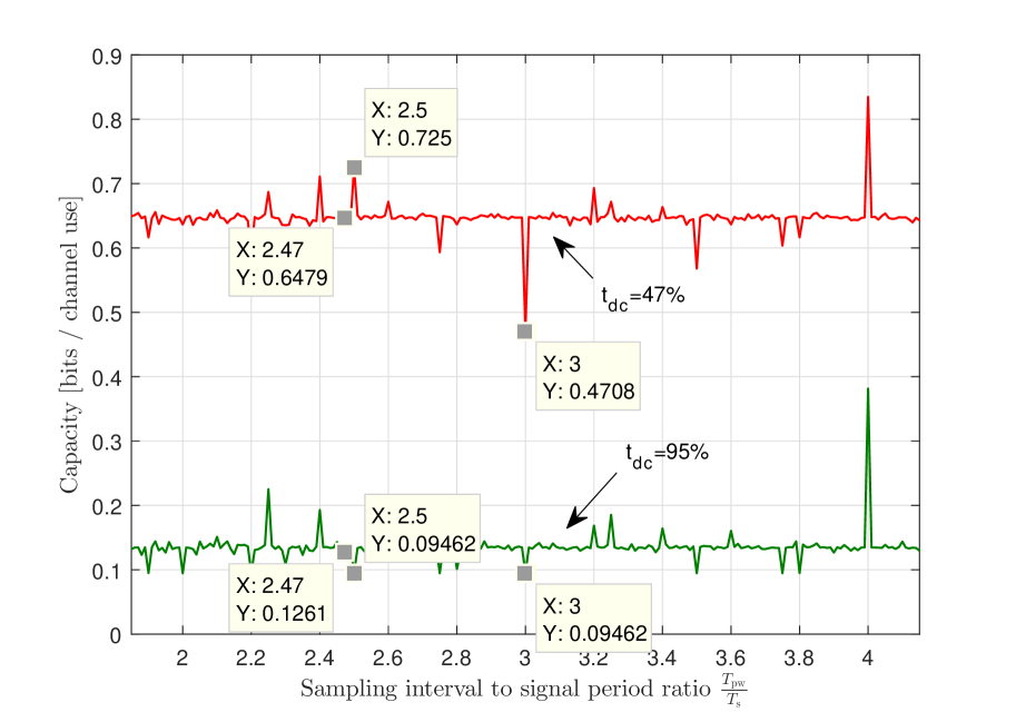
Figure 4: $C_{n}$ versus $\frac{T_{\rm pw}}{T_{\rm s}}$ for offset $\phi=0$.

    Figure 5: $C_{n}$ versus $\frac{T_{\rm pw}}{T_{\rm s}}$ for offset $\phi=\frac{1}{4}$.

To further demonstrate the assertion that minor variations in the sampling interval can lead to notable variations in capacity, we numerically evaluate the capacity versus the transmit power constraint $P$ for different values of synchronization mismatch $\epsilon$. In particular, we set $t_{\rm dc}=47\%$, fix $p=2$ and evaluate the capacity versus $P\in[1,100]$ for $\epsilon\in\{0,\frac{\pi}{1000},0.2\}$. Note that only $\epsilon=\frac{\pi}{1000}$ corresponds to asynchronous sampling, and that its sampling interval is approximately $2.496$ $\mu$secs, namely, a negligible variation from the sampling intervals corresponding to $\epsilon\in\{0,0.2\}$, which are $2.5$ $\mu$secs and $2.473$ $\mu$secs, respectively. The results of this numerical evaluation are depicted Figs. 7-7 for sampling offsets $\phi=0$ and $\phi=\frac{1}{4}$, respectively. Observing Figs. 7-7, we note that a change of less than $0.2\%$ in the sampling interval, corresponding to the synchronization mismatch $\epsilon$ changing from $\epsilon=0$ to $\epsilon=\frac{\pi}{1000}$, has a notable effect on capacity: At sampling offset $\phi=0$ such a change results in a dramatic decrease in capacity, e.g., at $P=10$ capacity decreases by roughly $30\%$. For $\phi=\frac{1}{4}$ such a change in the sampling rate slightly increases capacity. A similar behavior of a much smaller magnitude is observed comparing the curves corresponding to $\epsilon=0.2$ and $\epsilon=\frac{\pi}{1000}$. It is also noted that the capacity curve for the asynchronous sampling mismatch $\epsilon=\frac{\pi}{1000}$ is identical for both sampling offsets, indicating once again that when the sampling is asynchronous, capacity is invariant to sampling offsets.

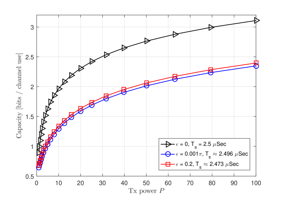
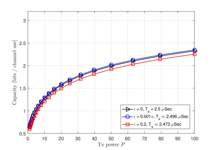
Figure 6: $C$ versus $P$ for $t_{\rm dc}=47\%$ and offset $\phi=0$.

    Figure 7: $C$ versus $P$ for $t_{\rm dc}=47\%$ and offset $\phi=\frac{1}{4}$.

In summary, the results presented above demonstrate that for DT memoryless channels with additive sampled CT WSCS noise, capacity can vary significantly between different sampling rates and sampling offsets. In particular, it is shown that when the sampling rate is not synchronized with the period of the WSCS noise, differently from the synchronized sampling case, capacity is not sensitive to sampling time offsets. It is also shown that capacity can change significantly due to minor variations in the sampling rate, especially when the variations cause the sampling rate to switch between synchronous and asynchronous sampling.

V Conclusions

In this work we characterized the capacity of DT memoryless communication channels with additive sampled WSCS Gaussian noise, a model which represents important scenarios, including interference-limited communications and cognitive communications. This model can be analyzed using common information-theoretic tools, e.g., methods based on the law of large numbers, only when the sampling rate is synchronized with the period of the noise statistics. To characterize its capacity with asynchronous sampling, we first derived a new relationship between the information spectrum quantities for uniformly convergent sequences of RVs. We then used this relationship to express the capacity of asynchronously-sampled memoryless additive WSCS Gaussian noise channels as the limit of a sequence of capacities of synchronously-sampled memoryless additive WSCS Gaussian noise channels. Our numerical analysis demonstrates how variations in the sampling rate, which switch the resulting model from synchronous sampling to asynchronous sampling, can significantly change capacity. In particular, it was shown that a small change of $0.2\%$ in the sampling rate caused a decrease of $30\%$ in capacity. Our characterization can be used, for example, to properly determine the sampling period in interference-limited communications such that capacity is maximized.

Appendix A Proof of Theorem 1

In the following we prove only (8a), as the proof of (8b) is obtained by following similar arguments. First, we note that Def. 3 can be written as

$${\rm p-}\mathop{\lim\inf}\limits_{k\rightarrow\infty}Z_{k}\!\stackrel{{\scriptstyle(a)}}{{=}}\!\sup\left\{\!\alpha\!\in\!\mathcal{R}\big{|}\mathop{\lim\sup}\limits_{k\rightarrow\infty}\Pr\left(Z_{k}\!<\!\alpha\right)\!\!=0\right\}\!=\!\sup\left\{\!\alpha\!\in\!\mathcal{R}\big{|}\mathop{\lim\sup}\limits_{k\rightarrow\infty}F_{k}(\alpha)\!=\!0\right\}.\vspace{-0.1cm}$$ (A.1)

For $(a)$ we first note that for a given $\alpha\in\mathcal{R}$, the non-negative sequence $\{\Pr\left(Z_{k}<\alpha\right)\}_{k\in\mathcal{N}}$ may not converge. Nonetheless, if for a given $\alpha$ it holds that $\mathop{\lim}\limits_{k\rightarrow\infty}\Pr\left(Z_{k}<\alpha\right)=0$, then for this value of $\alpha$ the limit exists and thus $\mathop{\lim\sup}\limits_{k\rightarrow\infty}\Pr\left(Z_{k}<\alpha\right)=0$. On the other hand, if for some $\alpha\in\mathcal{R}$ it holds that $\mathop{\lim\sup}\limits_{k\rightarrow\infty}\Pr\left(Z_{k}<\alpha\right)=0$, then, since $\{\Pr\left(Z_{k}<\alpha\right)\}_{k\in\mathcal{N}}$ is non negative, it holds that $\mathop{\lim\inf}\limits_{k\rightarrow\infty}\Pr\left(Z_{k}<\alpha\right)\geq 0$. Therefore by [35, Thm. 3.17] the limit exists and is equal to $\mathop{\lim}\limits_{k\rightarrow\infty}\Pr\left(Z_{k}<\alpha\right)=0$. We note that since $F_{k}(\alpha)\in[0,1]$, then, $\mathop{\lim\sup}\limits_{k\rightarrow\infty}F_{k}(\alpha)$ exists and is finite [35, Thm. 3.17], even if $\mathop{\lim}\limits_{k\rightarrow\infty}F_{k}(\alpha)$ does not exist.

The proof of Theorem 1 uses the following lemma:

Lemma A.1.

Given assumption AS2, for all $\alpha\in\mathcal{R}$ it holds that

$$\mathop{\lim\sup}\limits_{k\rightarrow\infty}F_{k}(\alpha)=\mathop{\lim}\limits_{n\rightarrow\infty}\mathop{\lim\sup}\limits_{k\rightarrow\infty}\tilde{F}_{k,n}(\alpha).\vspace{-0.1cm}$$ (A.2)

Proof:

To prove the lemma we first show that $\mathop{\lim\sup}\limits_{k\rightarrow\infty}F_{k}(\alpha)\leq\mathop{\lim}\limits_{n\rightarrow\infty}\mathop{\lim\sup}\limits_{k\rightarrow\infty}\tilde{F}_{k,n}(\alpha)$, and then we show $\mathop{\lim\sup}\limits_{k\rightarrow\infty}F_{k}(\alpha)\geq\mathop{\lim}\limits_{n\rightarrow\infty}\mathop{\lim\sup}\limits_{k\rightarrow\infty}\tilde{F}_{k,n}(\alpha)$. Recall that by AS2, for all $\alpha\in\mathcal{R}$ and $k\in\mathcal{N}$, $\tilde{F}_{k,n}(\alpha)$ converges as $n\rightarrow\infty$ to $F_{k}(\alpha)$, uniformly over $k$ and $\alpha$, i.e., for all $\eta>0$ there exists $n_{0}(\eta)\in\mathcal{N}$, $k_{0}\big{(}n_{0}(\eta),\eta\big{)}\in\mathcal{N}$ such that for every $n>n_{0}(\eta)$, $\alpha\in\mathcal{R}$ and $k>k_{0}\big{(}n_{0}(\eta),\eta\big{)}$, it holds that $\big{|}\tilde{F}_{k,n}(\alpha)-F_{k}(\alpha)\big{|}<\eta$. Consequently, for every subsequence $k_{1},k_{2},\ldots$ such that $\mathop{\lim}\limits_{l\rightarrow\infty}\tilde{F}_{k_{l},n}(\alpha)$ exists for any $n>n_{0}(\eta)$, it follows from [35, Thm. 7.11] that, as the convergence over $k$ is uniform, the limits over $n$ and $l$ are interchangeable:

$$\mathop{\lim}\limits_{n\rightarrow\infty}\mathop{\lim}\limits_{l\rightarrow\infty}\tilde{F}_{k_{l},n}(\alpha)=\mathop{\lim}\limits_{l\rightarrow\infty}\mathop{\lim}\limits_{n\rightarrow\infty}\tilde{F}_{k_{l},n}(\alpha)=\mathop{\lim}\limits_{l\rightarrow\infty}F_{k_{l}}(\alpha).\vspace{-0.1cm}$$ (A.3)

The existence of such a convergent subsequence is guaranteed by the Bolzano-Weierstrass Theorem [35, Thm. 2.42] as $\tilde{F}_{k,n}(\alpha)\in[0,1]$.

From the properties of the limit superior [35, Thm. 3.17] if follows that there exists a subsequence of $\big{\{}F_{k}(\alpha)\big{\}}_{k\in\mathcal{N}}$, denoted $\big{\{}F_{k_{m}}(\alpha)\big{\}}_{m\in\mathcal{N}}$, such that $\mathop{\lim}\limits_{m\rightarrow\infty}F_{k_{m}}(\alpha)=\mathop{\lim\sup}\limits_{k\rightarrow\infty}F_{k}(\alpha)$. Consequently,

$$\mathop{\lim\sup}\limits_{k\rightarrow\infty}F_{k}(\alpha) =\mathop{\lim}\limits_{m\rightarrow\infty}F_{k_{m}}(\alpha)\stackrel{{\scriptstyle(a)}}{{=}}\mathop{\lim}\limits_{n\rightarrow\infty}\mathop{\lim}\limits_{m\rightarrow\infty}\tilde{F}_{k_{m},n}(\alpha)$$

$$\stackrel{{\scriptstyle(b)}}{{\leq}}\mathop{\lim}\limits_{n\rightarrow\infty}\mathop{\lim\sup}\limits_{k\rightarrow\infty}\tilde{F}_{k,n}(\alpha),$$ (A.4)

where $(a)$ follows from (A.3), and $(b)$ follows from the definition of the limit superior [35, Def. 3.16].

Similarly, by [35, Thm. 3.17], for any $n\in\mathcal{N}$ there exists a subsequence $\big{\{}\tilde{F}_{m_{l},n}(\alpha)\big{\}}_{l\in\mathcal{N}}$ where $\{m_{l}\}_{l\in\mathcal{N}}$ satisfy $0<m_{1}<m_{2}<\ldots$, such that $\mathop{\lim}\limits_{l\rightarrow\infty}\tilde{F}_{m_{l},n}(\alpha)=\mathop{\lim\sup}\limits_{k\rightarrow\infty}\tilde{F}_{k,n}(\alpha)$. Therefore,

$$\mathop{\lim}\limits_{n\rightarrow\infty}\mathop{\lim\sup}\limits_{k\rightarrow\infty}\tilde{F}_{k,n}(\alpha) =\mathop{\lim}\limits_{n\rightarrow\infty}\mathop{\lim}\limits_{l\rightarrow\infty}\tilde{F}_{m_{l},n}(\alpha)$$

$$\stackrel{{\scriptstyle(a)}}{{=}}\mathop{\lim}\limits_{l\rightarrow\infty}F_{m_{l}}(\alpha)\stackrel{{\scriptstyle(b)}}{{\leq}}\mathop{\lim\sup}\limits_{k\rightarrow\infty}F_{k}(\alpha),$$ (A.5)

where $(a)$ follows from (A.3), and $(b)$ follows from the definition of the limit superior [35, Def. 3.16]. Therefore, $\mathop{\lim\sup}\limits_{k\rightarrow\infty}F_{k}(\alpha)\geq\mathop{\lim}\limits_{n\rightarrow\infty}\mathop{\lim\sup}\limits_{k\rightarrow\infty}\tilde{F}_{k,n}(\alpha)$. Combining (A.4) and (A.5) proves (A.2) in the statement of the lemma. ∎

Lemma A.2.

Under assumptions AS1-AS2, the sequence of RVs $\big{\{}\tilde{Z}_{k,n}\big{\}}_{k,n\in\mathcal{N}}$ satisfies

$$\mathop{\lim}\limits_{n\rightarrow\infty}\left({\rm p-}\mathop{\lim\inf}\limits_{k\rightarrow\infty}\tilde{Z}_{k,n}\right) =\sup\left\{\alpha\in\mathcal{R}\Big{|}\mathop{\lim}\limits_{n\rightarrow\infty}\mathop{\lim\sup}\limits_{k\rightarrow\infty}\tilde{F}_{k,n}(\alpha)=0\right\}.\vspace{-0.1cm}$$ (A.6)

Proof:

Since by assumption AS1, for every $n\in\mathcal{N}$, every convergent subsequence of $\big{\{}\tilde{Z}_{k,n}\big{\}}_{k\in\mathcal{N}}$ converges in distribution as $k\rightarrow\infty$ to a deterministic scalar, it follows that every convergent subsequence of $\tilde{F}_{k,n}(\alpha)$ converges as $k\rightarrow\infty$ to a step function, which is the CDF of the corresponding sublimit of $\tilde{Z}_{k,n}$. In particular, $\mathop{\lim\sup}\limits_{k\rightarrow\infty}\tilde{F}_{k,n}(\alpha)$ is a step function representing the CDF of the deterministic scalar $\zeta_{n}$, i.e.,

$$\mathop{\lim\sup}\limits_{k\rightarrow\infty}\tilde{F}_{k,n}(\alpha)=\begin{cases}0&\alpha\leq\zeta_{n}\\ 1&\alpha>\zeta_{n}.\end{cases}$$ (A.7)

Since, by Lemma A.1, AS2 implies that the limit $\mathop{\lim}\limits_{n\rightarrow\infty}\mathop{\lim\sup}\limits_{k\rightarrow\infty}\tilde{F}_{k,n}(\alpha)$ exists, then $\mathop{\lim}\limits_{n\rightarrow\infty}\zeta_{n}$ exists. Hence, we obtain that

$$\mathop{\lim}\limits_{n\rightarrow\infty}\mathop{\lim\sup}\limits_{k\rightarrow\infty}\tilde{F}_{k,n}(\alpha)=\begin{cases}0&\alpha\leq\mathop{\lim}\limits_{n\rightarrow\infty}\zeta_{n}\\ 1&\alpha>\mathop{\lim}\limits_{n\rightarrow\infty}\zeta_{n}.\end{cases}$$

It is emphasized that the equality in the above expression is arbitrary and does not affect the proof, i.e., while we wrote that $\mathop{\lim}\limits_{n\rightarrow\infty}\mathop{\lim\sup}\limits_{k\rightarrow\infty}\tilde{F}_{k,n}(\alpha)=0$ for $\alpha=\mathop{\lim}\limits_{n\rightarrow\infty}\zeta_{n}$, the proof holds also when $\mathop{\lim}\limits_{n\rightarrow\infty}\mathop{\lim\sup}\limits_{k\rightarrow\infty}\tilde{F}_{k,n}(\alpha)=1$ for $\alpha=\mathop{\lim}\limits_{n\rightarrow\infty}\zeta_{n}$. Consequently, the right-hand side of (A.6) equals to $\mathop{\lim}\limits_{n\rightarrow\infty}\zeta_{n}$.

Next, we note that

$${\rm p-}\mathop{\lim\inf}\limits_{k\rightarrow\infty}\tilde{Z}_{k,n}\stackrel{{\scriptstyle(a)}}{{=}}\sup\left\{\alpha\in\mathcal{R}\Big{|}\mathop{\lim\sup}\limits_{k\rightarrow\infty}\tilde{F}_{k,n}(\alpha)=0\right\}=\zeta_{n},$$

where $(a)$ follows from (A.1). Consequently, the left-hand side of (A.6) is equal to $\mathop{\lim}\limits_{n\rightarrow\infty}\zeta_{n}$, thus proving equality (A.6) in the statement of the lemma. ∎

Substituting (A.2) into (A.1) results in

$${\rm p-}\mathop{\lim\inf}\limits_{k\rightarrow\infty}Z_{k} =\sup\left\{\alpha\in\mathcal{R}\Big{|}\mathop{\lim}\limits_{n\rightarrow\infty}\mathop{\lim\sup}\limits_{k\rightarrow\infty}\tilde{F}_{k,n}(\alpha)=0\right\}\stackrel{{\scriptstyle(a)}}{{=}}\mathop{\lim}\limits_{n\rightarrow\infty}\left({\rm p-}\mathop{\lim\inf}\limits_{k\rightarrow\infty}\tilde{Z}_{k,n}\right),\vspace{-0.1cm}$$ (A.8)

where $(a)$ follows from (A.6). Eq. (A.8) proves (8a). Following similar arguments, we can prove (8b), thus concluding the proof of the theorem. ∎

Appendix B Proof of Theorem 2

The outline of the proof of Theorem 2 is as follows:

• First, we show in Subsection B-A that for any $k\in\mathcal{N}$, in the limit of $n\rightarrow\infty$, the PDF of ${{\boldsymbol{W}}}_{n}^{(k)}$ converges to the PDF of ${{\boldsymbol{W}}}_{\epsilon}^{(k)}$, and that convergence is uniform with respect to $k\in\mathcal{N}$ and to the realization ${\boldsymbol{w}}^{(k)}\in\mathcal{R}^{k}$. This is stated in Lemma B.1.

• Next, in Subsection B-B we use Theorem 1 to relate the mutual information density rates of the channels (3) and (12). To properly state the relationship proved in Subsection B-B, let $F_{{{\boldsymbol{X}}}}$ denote the distribution of the stochastic process $\{X[i]\}_{i\in\mathcal{N}}$, i.e., $F_{{{\boldsymbol{X}}}}\equiv\left\{F_{{{\boldsymbol{X}}}^{(k)}}\right\}_{k=1}^{\infty}$ is the set of CDFs of all random vectors ${{\boldsymbol{X}}}^{(k)}$ whose entries are the elements of $\{X[i]\}_{i\in\mathcal{N}}$ [36, Ch. 10.1]. We define the following random functions:

  $$Z_{k}^{\prime}\left(F_{{{\boldsymbol{X}}}}\right)\triangleq\frac{1}{k}\log\frac{p_{{{\boldsymbol{Y}}}_{\epsilon}^{(k)}|{{\boldsymbol{X}}}^{(k)}}\left({{\boldsymbol{Y}}}_{\epsilon}^{(k)}\big{|}{{\boldsymbol{X}}}^{(k)}\right)}{p_{{{\boldsymbol{Y}}}_{\epsilon}^{(k)}}\left({{\boldsymbol{Y}}}_{\epsilon}^{(k)}\right)},$$ (B.1a)

  and

  $$\tilde{Z}_{k,n}^{\prime}\left(F_{{{\boldsymbol{X}}}}\right)\triangleq\frac{1}{k}\log\frac{p_{{{\boldsymbol{Y}}}_{n}^{(k)}|{{\boldsymbol{X}}}^{(k)}}\left({{\boldsymbol{Y}}}_{n}^{(k)}\big{|}{{\boldsymbol{X}}}^{(k)}\right)}{p_{{{\boldsymbol{Y}}}_{n}^{(k)}}\left({{\boldsymbol{Y}}}_{n}^{(k)}\right)},$$ (B.1b)

  $k,n\in\mathcal{N}$. Note that the RVs in (B.1) represent the mutual information density rates [28, Def. 3.2.1] for the sampled channel (3) and for the additive WSCS noise channel (12), respectively, with a given input distribution. In Lemma B.2 we show that if the Gaussian random vectors ${{\boldsymbol{X}}}_{n}^{(k)}$ and ${{\boldsymbol{X}}}^{(k)}$ satisfy that ${{\boldsymbol{X}}}_{n}^{(k)}\mathop{\longrightarrow}\limits^{(dist.)}_{n\rightarrow\infty}{{\boldsymbol{X}}}^{(k)}$ uniformly with respect to $k$, then $\tilde{Z}_{k,n}^{\prime}\left(F_{{{\boldsymbol{X}}}_{n}}\right)\mathop{\longrightarrow}\limits^{(dist.)}_{n\rightarrow\infty}Z_{k}^{\prime}\left(F_{{{\boldsymbol{X}}}}\right)$ uniformly in $k\in\mathcal{N}$. Subsequently, Lemma B.3 proves that every subsequence of $\tilde{Z}_{k,n}^{\prime}\left(F_{{{\boldsymbol{X}}}}\right)$ converges in distribution to a deterministic scalar.

• Finally, in Subsection B-C, we combine the above results and show in Lemmas B.5 and B.6 that $C_{\epsilon}\geq\mathop{\lim\inf}\limits_{n\rightarrow\infty}C_{n}$ and $C_{\epsilon}\leq\mathop{\lim\inf}\limits_{n\rightarrow\infty}C_{n}$, respectively, concluding that $C_{\epsilon}=\mathop{\lim\inf}\limits_{n\rightarrow\infty}C_{n}$.

We henceforth assume that $\frac{1}{2\pi}<\sigma^{2}_{W_{\rm c}}(t)<\infty$ for all $t\in\mathcal{R}$. The motivation for this assumption is that it allows us to show that ${{\boldsymbol{W}}}_{n}^{(k)}$ converges uniformly to ${\boldsymbol{W}}_{\epsilon}^{(k)}$, without having to consider the power of the information signal. Note that this assumption has no effect on the generality of our capacity derivation, since multiplying $\{Y_{\epsilon}[i]\}_{i\in\mathcal{N}}$ by some positive constant $\kappa$ is an invertible transformation hence it does not affect capacity. Consequently, the capacity of the channel (3) subject to an average power constraint $P$ is identical to the capacity of a channel whose output is given by $X[i]+\kappa\cdot W_{\epsilon}[i]$ subject to an average power constraint $\kappa^{2}P$. Therefore, if there exists $t_{0}\in\mathcal{R}$ for which $\sigma^{2}_{W_{\rm c}}(t_{0})\leq\frac{1}{2\pi}$, then one can obtain a channel with the same capacity which satisfies the assumption above by properly scaling the output signal and the power constraint.

B-A Convergence in Distribution of ${{\boldsymbol{W}}}_{n}^{(k)}$ to ${{\boldsymbol{W}}}_{\epsilon}^{(k)}$ Uniformly with respect to $k\in\mathcal{N}$

To prove that ${{\boldsymbol{W}}}_{n}^{(k)}$ converges in distribution to ${{\boldsymbol{W}}}_{\epsilon}^{(k)}$ as $n\rightarrow\infty$ uniformly with respect to $k\in\mathcal{N}$, we first prove in Lemma B.1 that the PDF of ${{\boldsymbol{W}}}_{n}^{(k)}$ converges to the PDF of ${{\boldsymbol{W}}}_{\epsilon}^{(k)}$ uniformly in $k$. We then conclude in Corollary B.1 that ${{\boldsymbol{W}}}_{n}^{(k)}\mathop{\longrightarrow}\limits^{(dist.)}_{n\rightarrow\infty}{{\boldsymbol{W}}}_{\epsilon}^{(k)}$ uniformly in $k\in\mathcal{N}$.

Define the set $\mathcal{K}\triangleq\{1,2,...,k\}$, and consider the zero-mean random vectors of dimension $k$: ${{\boldsymbol{W}}}_{n}^{(k)}$ and ${{\boldsymbol{W}}}_{\epsilon}^{(k)}$. Let $\mathsf{C}_{\epsilon}^{k}$ and $\mathsf{C}_{n}^{k}$ denote the correlation matrices:

$$\mathsf{C}_{\epsilon}^{k} \triangleq \mathds{E}\left\{({{\boldsymbol{W}}}_{\epsilon}^{(k)})({{\boldsymbol{W}}}_{\epsilon}^{(k)})^{T}\right\}\equiv{\rm diag}\left(\sigma^{2}_{W_{\epsilon}}[1],\ldots,\sigma^{2}_{W_{\epsilon}}[k]\right)$$ (B.2a)

$$\mathsf{C}_{n}^{k} \triangleq \mathds{E}\left\{({{\boldsymbol{W}}}_{n}^{(k)})({{\boldsymbol{W}}}_{n}^{(k)})^{T}\right\}\equiv{\rm diag}\left(\sigma^{2}_{W_{n}}[1],\ldots,\sigma^{2}_{W_{n}}[k]\right),$$ (B.2b)

where ${\rm diag}(m_{1},m_{2},\ldots,m_{l})$ denotes an $l\times l$ diagonal matrix with the specified elements, i.e., letting $\mathsf{M}={\rm diag}(m_{1},m_{2},\ldots,m_{l})$ then $\left(\mathsf{M}\right)_{i,i}=m_{i}$. We can now state the following lemma:

Lemma B.1.

As $n\rightarrow\infty$, the PDF of ${{\boldsymbol{W}}}_{n}^{(k)}$ converges uniformly in ${{\boldsymbol{w}}}^{(k)}\in\mathcal{R}^{k}$ and in $k\in\mathcal{N}$ to the PDF of ${{\boldsymbol{W}}}_{\epsilon}^{(k)}$:

$$\lim_{n\rightarrow\infty}p_{{{\boldsymbol{W}}}_{n}^{(k)}}\big{(}{{\boldsymbol{w}}}^{(k)}\big{)}=p_{{{\boldsymbol{W}}}_{\epsilon}^{(k)}}\big{(}{{\boldsymbol{w}}}^{(k)}\big{)},\qquad\forall{{\boldsymbol{w}}}^{(k)}\in\mathcal{R}^{k},\forall k\in\mathcal{N}.\vspace{-0.1cm}$$

Proof:

To prove the lemma, we first fix $k\in\mathcal{N}$, and show that $p_{{{\boldsymbol{W}}}_{n}^{(k)}}\big{(}{{\boldsymbol{w}}}^{(k)}\big{)}$ converges to $p_{{{\boldsymbol{W}}}_{\epsilon}^{(k)}}\big{(}{{\boldsymbol{w}}}^{(k)}\big{)}$ uniformly in ${{\boldsymbol{w}}}^{(k)}\in\mathcal{R}^{k}$. Then, we prove that this convergence is uniform in $k$.

We start by recalling that ${{\boldsymbol{W}}}_{n}^{(k)}$ and ${{\boldsymbol{W}}}_{\epsilon}^{(k)}$ have independent entries, and by noting that since $\epsilon_{n}\triangleq\frac{1}{n}\cdot\lfloor n\cdot\epsilon\rfloor$ it holds that $\frac{n\epsilon-1}{n}\leq\epsilon_{n}\leq\frac{n\epsilon}{n}$, hence,

$$\lim_{n\rightarrow\infty}\epsilon_{n}=\epsilon.$$ (B.3)

Note that since $\sigma^{2}_{W_{\rm c}}(t)$ is a uniformly continuous function, then by the definition of a uniformly continuous function, for each $i\in\mathcal{N}$ (B.3) implies that

$$\lim_{n\rightarrow\infty}\sigma^{2}_{W_{n}}[i]=\lim_{n\rightarrow\infty}\sigma^{2}_{W_{\rm c}}\left(i\cdot\frac{T_{\rm pw}}{p+\epsilon_{n}}\right)=\sigma^{2}_{W_{\rm c}}\left(i\cdot\frac{T_{\rm pw}}{p+\epsilon}\right)\equiv\sigma^{2}_{W_{\epsilon}}[i].$$ (B.4)

Now, from the definitions of the correlation matrices $\mathsf{C}_{\epsilon}^{k}$ and $\mathsf{C}_{n}^{k}$, we have that

$$\lim_{n\rightarrow\infty}\max_{(u,v)\in\mathcal{K}\times\mathcal{K}}\left\{\left|\left(\mathsf{C}_{n}^{k}\right)_{u,v}-\left(\mathsf{C}_{\epsilon}^{k}\right)_{u,v}\right|\right\}=\lim_{n\rightarrow\infty}\max_{i\in\mathcal{K}}\left\{\left|\sigma^{2}_{W_{n}}[i]-\sigma^{2}_{W_{\epsilon}}[i]\right|\right\}=0.\vspace{-0.1cm}$$ (B.5)

Next, define the $k\times k$ diagonal matrix $\mathsf{C}^{k}$, the real vector ${{\boldsymbol{w}}}^{(k)}\in\mathcal{R}^{k}$, and the mappings $\mathds{M}^{(1)}_{k}$, $\mathds{M}^{(2)}_{k}$, and $\mathds{M}_{k}$ as follows: The mapping

$$\mathds{M}^{(1)}_{k}:\mathcal{R}^{k^{2}}\mapsto\mathcal{R}$$

is defined as

$$\mathds{M}^{(1)}_{k}\big{(}\mathsf{C}^{k}\big{)}={\rm Det}\big{(}\mathsf{C}^{k}\big{)}\stackrel{{\scriptstyle(a)}}{{=}}\prod_{i=1}^{k}\left(\mathsf{C}^{k}\right)_{i,i},$$

where $(a)$ follows from the fact that $\mathsf{C}^{k}$ is diagonal [46, Ch. 6.1]. Obviously, the function $\mathds{M}_{k}^{(1)}\big{(}\mathsf{C}^{k}\big{)}$ is continuous in $\mathsf{C}^{k}$.

The mapping

$$\mathds{M}^{(2)}_{k}:\mathcal{R}^{k^{2}}\mapsto\mathcal{R}^{k^{2}}$$

is next defined via

$$\mathds{M}^{(2)}_{k}\big{(}\mathsf{C}^{k}\big{)}=\big{(}\mathsf{C}^{k}\big{)}^{-1}.$$

Note that $\mathds{M}^{(2)}_{k}\big{(}\mathsf{C}^{k}\big{)}$ is a continuous mapping, see, e.g., [45].

Finally, consider the mapping

$$\mathds{M}_{k}:\mathcal{R}^{k^{2}}\times\mathcal{R}^{k}\mapsto\mathcal{R}$$

via

$$\mathds{M}_{k}\big{(}\mathsf{C}^{k},{{\boldsymbol{w}}}^{(k)}\big{)}=(2\pi)^{-k/2}\Big{(}{\rm Det}\big{(}\mathsf{C}^{k}\big{)}\Big{)}^{-1/2}\cdot\exp\left(-\frac{1}{2}\big{(}{{\boldsymbol{w}}}^{(k)}\big{)}^{T}\big{(}\mathsf{C}^{k}\big{)}^{-1}{{\boldsymbol{w}}}^{(k)}\right).$$

Since the composition of continuous functions is a continuous function [44, Thm. 11.2.3], it follows that $\exp\Big{(}-\frac{1}{2}\big{(}{{\boldsymbol{w}}}^{(k)}\big{)}^{T}\big{(}\mathsf{C}^{k}\big{)}^{-1}{{\boldsymbol{w}}}^{(k)}\Big{)}$ is a continuous function in $\mathsf{C}^{k}$ and ${{\boldsymbol{w}}}^{(k)}$, and hence $\mathds{M}_{k}$ is the product of two continuous functions, from which it follows that $\mathds{M}_{k}$ is a continuous mapping in $\mathsf{C}^{k}$ and ${{\boldsymbol{w}}}^{(k)}$. Furthermore, we note that for diagonal non-singular $\mathsf{C}^{k}$, it holds that

$$\exp\Big{(}-\frac{1}{2}\big{(}{{\boldsymbol{w}}}^{(k)}\big{)}^{T}\big{(}\mathsf{C}^{k}\big{)}^{-1}{{\boldsymbol{w}}}^{(k)}\Big{)}=\prod\limits_{i=1}^{k}\exp\left(-\frac{\left({{\boldsymbol{w}}}^{(k)}\right)_{i}^{2}}{2\left(\mathsf{C}^{k}\right)_{i,i}}\right),$$

is uniformly continuous in ${{\boldsymbol{w}}}^{(k)}\in\mathcal{R}^{k}$ [35, Thm. 5.10]. It thus follows from (B.5) and from [44, Thm. 11.2.3] that $\mathop{\lim}\limits_{n\rightarrow\infty}\mathds{M}_{k}\big{(}\mathsf{C}_{n}^{k},{{\boldsymbol{w}}}^{(k)}\big{)}=\mathds{M}_{k}\big{(}\mathsf{C}_{\epsilon}^{k},{{\boldsymbol{w}}}^{(k)}\big{)}$.

Noting that $p_{{{\boldsymbol{W}}}_{n}^{(k)}}\big{(}{{\boldsymbol{w}}}^{(k)}\big{)}=\mathds{M}_{k}\big{(}\mathsf{C}_{n}^{k},{{\boldsymbol{w}}}^{(k)}\big{)}$ and $p_{{{\boldsymbol{W}}}_{\epsilon}^{(k)}}\big{(}{{\boldsymbol{w}}}^{(k)}\big{)}=\mathds{M}_{k}\big{(}\mathsf{C}_{\epsilon}^{k},{{\boldsymbol{w}}}^{(k)}\big{)}$, proves that for a given $k\in\mathcal{N}$, the sequence of PDFs $p_{{{\boldsymbol{W}}}_{n}^{(k)}}\big{(}{{\boldsymbol{w}}}^{(k)}\big{)}$ converges pointwise as $n\rightarrow\infty$, for each ${{\boldsymbol{w}}}^{(k)}\in\mathcal{R}^{k}$ .

To see that this convergence is uniform in ${{\boldsymbol{w}}}^{(k)}\in\mathcal{R}^{k}$, we note that the sequence of zero-mean multivariate Gaussian PDFs satisfy that $\forall\eta>0$ and $\forall n_{0}(k)\in\mathcal{N}$ there exists some $r\big{(}\eta,n_{0}(k)\big{)}>0$ such that $\max\left\{p_{{{\boldsymbol{W}}}_{n}^{(k)}}\big{(}{{\boldsymbol{w}}}^{(k)}\big{)},p_{{{\boldsymbol{W}}}_{\epsilon}^{(k)}}\big{(}{{\boldsymbol{w}}}^{(k)}\big{)}\right\}<\eta$, for all ${{\boldsymbol{w}}}^{(k)}\in\mathcal{R}^{k}$ satisfying $\|{{\boldsymbol{w}}}^{(k)}\|>r\big{(}\eta,n_{0}(k)\big{)}$ and for all $n>n_{0}(k)$. Thus $\Big{|}p_{{{\boldsymbol{W}}}_{n}^{(k)}}\big{(}{{\boldsymbol{w}}}^{(k)}\big{)}-p_{{{\boldsymbol{W}}}_{\epsilon}^{(k)}}\big{(}{{\boldsymbol{w}}}^{(k)}\big{)}\Big{|}<\eta$, for all ${{\boldsymbol{w}}}^{(k)}\in\mathcal{R}^{k}$ satisfying $\|{{\boldsymbol{w}}}^{(k)}\|>r\big{(}\eta,n_{0}(k)\big{)}$ and for all $n>n_{0}(k)$. Since $p_{{{\boldsymbol{W}}}_{n}^{(k)}}\big{(}{{\boldsymbol{w}}}^{(k)}\big{)}$ converges pointwise to $p_{{{\boldsymbol{W}}}_{\epsilon}^{(k)}}\big{(}{{\boldsymbol{w}}}^{(k)}\big{)}$ as $n\rightarrow\infty$, it follows from the uniform continuity of $p_{{{\boldsymbol{W}}}_{n}^{(k)}}\big{(}{{\boldsymbol{w}}}^{(k)}\big{)}$ and $p_{{{\boldsymbol{W}}}_{\epsilon}^{(k)}}\big{(}{{\boldsymbol{w}}}^{(k)}\big{)}$ that $\exists\tilde{n}_{0}(\eta,k)>0$ (independent of ${{\boldsymbol{w}}}^{(k)}\in\mathcal{R}^{k}$) such that for all $n>\tilde{n}_{0}(\eta,k)$ then $\left|p_{{{\boldsymbol{W}}}_{n}^{(k)}}\big{(}{{\boldsymbol{w}}}^{(k)}\big{)}-p_{{{\boldsymbol{W}}}_{\epsilon}^{(k)}}\big{(}{{\boldsymbol{w}}}^{(k)}\big{)}\right|<\eta$ for all ${{\boldsymbol{w}}}^{(k)}\in\mathcal{R}^{k}$ in the closed set $\|{{\boldsymbol{w}}}^{(k)}\|\leq r\big{(}\eta,n_{0}(k)\big{)}$. This is obtained by noting that for $\|{{\boldsymbol{w}}}^{(k)}\|\leq r\big{(}\eta,n_{0}(k)\big{)}$, the difference $\left|p_{{{\boldsymbol{W}}}_{n}^{(k)}}\big{(}{{\boldsymbol{w}}}^{(k)}\big{)}-p_{{{\boldsymbol{W}}}_{\epsilon}^{(k)}}\big{(}{{\boldsymbol{w}}}^{(k)}\big{)}\right|$ attains a maximal values. This value can be made arbitrarily small do to the continuity of the PDFs in ${{\boldsymbol{w}}}^{(k)}\in\mathcal{R}^{k}$. Note also that due to convergence, the difference $\left|p_{{{\boldsymbol{W}}}_{n}^{(k)}}\big{(}{{\boldsymbol{w}}}^{(k)}\big{)}-p_{{{\boldsymbol{W}}}_{\epsilon}^{(k)}}\big{(}{{\boldsymbol{w}}}^{(k)}\big{)}\right|$ decreases also for $\|{{\boldsymbol{w}}}^{(k)}\|>r\big{(}\eta,n_{0}(k)\big{)}$. Consequently, $\left|p_{{{\boldsymbol{W}}}_{n}^{(k)}}\big{(}{{\boldsymbol{w}}}^{(k)}\big{)}-p_{{{\boldsymbol{W}}}_{\epsilon}^{(k)}}\big{(}{{\boldsymbol{w}}}^{(k)}\big{)}\right|<\eta$ for all $n>\max\big{\{}\tilde{n}_{0}(\eta,k),n_{0}(k)\big{\}}$ and for each ${{\boldsymbol{w}}}^{(k)}\in\mathcal{R}^{k}$, and thus convergence is uniform in ${{\boldsymbol{w}}}^{(k)}\in\mathcal{R}^{k}$.

Next, we prove that the convergence is uniform in $k$. To that aim, we fix $\eta>0$ and $k_{0}\in\mathcal{N}$, and prove that $\exists n_{0}(\eta,k_{0})$ such that for all $n>n_{0}(\eta,k_{0})$ and for all sufficiently large $k$, it holds that $\big{|}p_{{{\boldsymbol{W}}}_{n}^{(k)}}\big{(}{{\boldsymbol{w}}}^{(k)}\big{)}-p_{{{\boldsymbol{W}}}_{\epsilon}^{(k)}}\big{(}{{\boldsymbol{w}}}^{(k)}\big{)}\big{|}<\eta$ for every ${{\boldsymbol{w}}}^{(k)}\in\mathcal{R}^{k}$. Since $n_{0}(\eta,k_{0})$ does not depend on $k$ (only on the fixed $k_{0}$), this implies that the convergence is uniform with respect to $k\in\mathcal{N}$.

To that aim we first note that since the sequence of PDFs $p_{{{\boldsymbol{W}}}_{n}^{(k_{0})}}\big{(}{{\boldsymbol{w}}}^{(k_{0})}\big{)}$ converges as $n\rightarrow\infty$ to $p_{{{\boldsymbol{W}}}_{\epsilon}^{(k_{0})}}\big{(}{{\boldsymbol{w}}}^{(k_{0})}\big{)}$ uniformly in ${{\boldsymbol{w}}}^{(k_{0})}\in\mathcal{R}^{k_{0}}$, it follows that $\exists n_{0}(\eta,k_{0})\in\mathcal{N}$ such that for all $n>n_{0}(\eta,k_{0})$ and for all ${{\boldsymbol{w}}}^{(k_{0})}\in\mathcal{R}^{k_{0}}$, it holds that

$$\big{|}p_{{{\boldsymbol{W}}}_{n}^{(k_{0})}}\big{(}{{\boldsymbol{w}}}^{(k_{0})}\big{)}-p_{{{\boldsymbol{W}}}_{\epsilon}^{(k_{0})}}\big{(}{{\boldsymbol{w}}}^{(k_{0})}\big{)}\big{|}<\frac{\eta}{2}.$$

Thus, for all $k>k_{0}$ and for all ${{\boldsymbol{w}}}^{(k)}\in\mathcal{R}^{k}$, using the notation $w_{i}\triangleq\big{(}{{\boldsymbol{w}}}^{(k)}\big{)}_{i}$, we can write

$$\left|p_{{{\boldsymbol{W}}}_{n}^{(k)}}\Big{(}{{\boldsymbol{w}}}^{(k)}\Big{)}\!-\!p_{{{\boldsymbol{W}}}_{\epsilon}^{(k)}}\Big{(}{{\boldsymbol{w}}}^{(k)}\Big{)}\right| =\left|p_{{{\boldsymbol{W}}}_{n}^{(k_{0})}}\Big{(}{{\boldsymbol{w}}}^{(k_{0})}\Big{)}\prod\limits_{i=k_{0}+1}^{k}p_{W_{n}[i]}\left(w_{i}\right)\!-\!p_{{{\boldsymbol{W}}}_{\epsilon}^{(k_{0})}}\Big{(}{{\boldsymbol{w}}}^{(k_{0})}\Big{)}\prod\limits_{i=k_{0}+1}^{k}p_{W_{\epsilon}[i]}\left(w_{i}\right)\right|$$

$$=\Bigg{|}p_{{{\boldsymbol{W}}}_{n}^{(k_{0})}}\Big{(}{{\boldsymbol{w}}}^{(k_{0})}\Big{)}\left(\prod\limits_{i=k_{0}+1}^{k}p_{W_{n}[i]}\left(w_{i}\right)\!-\!\prod\limits_{i=k_{0}+1}^{k}p_{W_{\epsilon}[i]}\left(w_{i}\right)\right)$$

$$\quad+\left(p_{{{\boldsymbol{W}}}_{n}^{(k_{0})}}\Big{(}{{\boldsymbol{w}}}^{(k_{0})}\Big{)}\!-\!p_{{{\boldsymbol{W}}}_{\epsilon}^{(k_{0})}}\Big{(}{{\boldsymbol{w}}}^{(k_{0})}\Big{)}\right)\prod\limits_{i=k_{0}+1}^{k}p_{W_{\epsilon}[i]}\left(w_{i}\right)\Bigg{|}$$

$$\leq p_{{{\boldsymbol{W}}}_{n}^{(k_{0})}}\Big{(}{{\boldsymbol{w}}}^{(k_{0})}\Big{)}\left|\prod\limits_{i=k_{0}+1}^{k}p_{W_{n}[i]}\left(w_{i}\right)\!-\!\prod\limits_{i=k_{0}+1}^{k}p_{W_{\epsilon}[i]}\left(w_{i}\right)\right|$$

$$\quad+\prod\limits_{i=k_{0}+1}^{k}p_{W_{\epsilon}[i]}\left(w_{i}\right)\left|p_{{{\boldsymbol{W}}}_{n}^{(k_{0})}}\Big{(}{{\boldsymbol{w}}}^{(k_{0})}\Big{)}\!-\!p_{{{\boldsymbol{W}}}_{\epsilon}^{(k_{0})}}\Big{(}{{\boldsymbol{w}}}^{(k_{0})}\Big{)}\right|.$$ (B.6)

Next, by defining the subset $\mathcal{P}\triangleq[0,T_{\rm pw}]\subset\mathcal{R}$, we note that the Gaussian PDF satisfies

$$p_{W_{n}[i]}(w_{i}) \leq\sqrt{\frac{1}{2\pi\cdot\sigma^{2}_{W_{n}}[i]}}\stackrel{{\scriptstyle(a)}}{{\leq}}\sqrt{\frac{1}{2\pi\cdot\mathop{\min}\limits_{t\in\mathcal{R}}\sigma^{2}_{W_{\rm c}}(t)}}\stackrel{{\scriptstyle(b)}}{{=}}\sqrt{\frac{1}{2\pi\cdot\mathop{\min}\limits_{t\in\mathcal{P}}\sigma^{2}_{W_{\rm c}}(t)}}\stackrel{{\scriptstyle(c)}}{{<}}1,$$ (B.7)

$\forall w_{i}\in\mathcal{R}$. Here, $(a)$ follows from (11), $(b)$ follows since $W_{\rm c}(t)$ is WSCS with period $T_{\rm pw}$, and $(c)$ follows from the assumption $\sigma^{2}_{W_{\rm c}}(t)>\frac{1}{2\pi}$. Similarly, $p_{W_{\epsilon}[i]}(w_{i})<1$ for all $w_{i}\in\mathcal{R}$. It follows from (B.7) that $\exists k_{1}(\eta)>0$ (independent of $n$) such that for all $k>k_{1}(\eta)$, $\prod\limits_{i=k_{0}+1}^{k}p_{W_{n}[i]}\left(w_{i}\right)<\frac{\eta}{2}$ and $\prod\limits_{i=k_{0}+1}^{k}p_{W_{\epsilon}[i]}\left(w_{i}\right)<\frac{\eta}{2}$, for all ${{\boldsymbol{w}}}^{(k)}\in\mathcal{R}^{k}$. Furthermore, (B.7) also implies that $p_{{{\boldsymbol{W}}}_{n}^{(k_{0})}}\big{(}{{\boldsymbol{w}}}^{(k_{0})}\big{)}<1$. Plugging these inequalities into (B.6) results in

$$\left|p_{{{\boldsymbol{W}}}_{n}^{(k)}}\big{(}{{\boldsymbol{w}}}^{(k)}\big{)}-p_{{{\boldsymbol{W}}}_{\epsilon}^{(k)}}\big{(}{{\boldsymbol{w}}}^{(k)}\big{)}\right| \leq\frac{\eta}{2}+\frac{\eta}{2}\left|p_{{{\boldsymbol{W}}}_{n}^{(k_{0})}}\big{(}{{\boldsymbol{w}}}^{(k_{0})}\big{)}-p_{{{\boldsymbol{W}}}_{\epsilon}^{(k_{0})}}\big{(}{{\boldsymbol{w}}}^{(k_{0})}\big{)}\right|\leq\frac{\eta}{2}\left(\frac{\eta}{2}+1\right),$$ (B.8)

$\forall{{\boldsymbol{w}}}^{(k)}\in\mathcal{R}^{k}$. Eqn. (B.8) implies that for all sufficiently small $\eta<1$, if $n>n_{0}(\eta,k_{0})$, then $\big{|}p_{{{\boldsymbol{W}}}_{n}^{(k)}}\big{(}{{\boldsymbol{w}}}^{(k)}\big{)}-p_{{{\boldsymbol{W}}}_{\epsilon}^{(k)}}\big{(}{{\boldsymbol{w}}}^{(k)}\big{)}\big{|}<\eta$ for all ${{\boldsymbol{w}}}^{(k)}\in\mathcal{R}^{k}$ and for all sufficiently large $k\in\mathcal{N}$, thus concluding the proof of the lemma. ∎

Corollary B.1.

For any $k\in\mathcal{N}$ it holds that ${{\boldsymbol{W}}}_{n}^{(k)}\mathop{\longrightarrow}\limits^{(dist.)}_{n\rightarrow\infty}{{\boldsymbol{W}}}_{\epsilon}^{(k)}$, uniformly over $k$.

Proof:

Since the continuous PDF of the continuous random vector ${{\boldsymbol{W}}}_{n}^{(k)}$ converges to the continuous PDF of continuous random vector ${{\boldsymbol{W}}}_{\epsilon}^{(k)}$, it follows from [40, Thm. 1] that ${{\boldsymbol{W}}}_{n}^{(k)}\mathop{\longrightarrow}\limits^{(dist.)}_{n\rightarrow\infty}{{\boldsymbol{W}}}_{\epsilon}^{(k)}$. Since the convergence of the PDFs is uniform in $k\in\mathcal{N}$, the convergence of the CDFs is also uniform by [40, Thm. 1]. ∎

B-B Showing that $\tilde{Z}_{k,n}^{\prime}\left(F_{{{\boldsymbol{X}}}_{n}}\right)$ and $Z_{k}^{\prime}\left(F_{{{\boldsymbol{X}}}}\right)$ Satisfy the Conditions of Thm. 1

Let $F_{{{\boldsymbol{X}}}_{n}}^{\rm opt}$ denote the optimal input distribution for the channel (12) subject to the input power constraint (4). We next prove that $\tilde{Z}_{k,n}^{\prime}\left(F_{{{\boldsymbol{X}}}_{n}}\right)$ and $Z_{k}^{\prime}\left(F_{{{\boldsymbol{X}}}}\right)$ satisfy AS1-AS2. In particular, Lemma B.2 proves that $\tilde{Z}_{k,n}^{\prime}\left(F_{{{\boldsymbol{X}}}_{n}}\right)\mathop{\longrightarrow}\limits^{(dist.)}_{n\rightarrow\infty}Z_{k}^{\prime}\left(F_{{{\boldsymbol{X}}}}\right)$ uniformly in $k\in\mathcal{N}$ for zero-mean Gaussian input vectors with independent entries. Lemma B.3 proves that for $k\rightarrow\infty$, $\tilde{Z}_{k,n}^{\prime}\left(F_{{{\boldsymbol{X}}}_{n}}^{\rm opt}\right)$ converges in distribution to a deterministic scalar.

Lemma B.2.

Consider a sequence of $k\times 1$ zero-mean Gaussian random vectors with independent entries $\{{{\boldsymbol{X}}}_{n}^{(k)}\}_{n\in\mathcal{N}}$ and a zero-mean Gaussian random vector with independent entries ${{\boldsymbol{X}}}^{(k)}$, such that ${{\boldsymbol{X}}}_{n}^{(k)}\mathop{\longrightarrow}\limits^{(dist.)}_{n\rightarrow\infty}{{\boldsymbol{X}}}^{(k)}$ uniformly with respect to $k\in\mathcal{N}$. Then, the RVs $\tilde{Z}_{k,n}^{\prime}\left(F_{{{\boldsymbol{X}}}_{n}}\right)$ and $Z_{k}^{\prime}\left(F_{{{\boldsymbol{X}}}}\right)$ defined in (B.1) satisfy $\tilde{Z}_{k,n}^{\prime}\left(F_{{{\boldsymbol{X}}}_{n}}\right)\mathop{\longrightarrow}\limits^{(dist.)}_{n\rightarrow\infty}Z_{k}^{\prime}\left(F_{{{\boldsymbol{X}}}}\right)$ uniformly over $k\in\mathcal{N}$.

Proof:

For ${\bf y}^{(k)},{\bf x}^{(k)}\in\mathcal{R}^{k}$, define

$$f_{k,n}\left(\mathbf{y}^{(k)},{\bf x}^{(k)}\right)\triangleq\frac{p_{{{\boldsymbol{Y}}}_{n}^{(k)}|{{\boldsymbol{X}}}_{n}^{(k)}}\left(\mathbf{y}^{(k)}\big{|}\mathbf{x}^{(k)}\right)}{p_{{{\boldsymbol{Y}}}_{n}^{(k)}}\left(\mathbf{y}^{(k)}\right)},\qquad f_{k,\epsilon}\left(\mathbf{y}^{(k)},\mathbf{x}^{(k)}\right)\triangleq\frac{p_{{{\boldsymbol{Y}}}_{\epsilon}^{(k)}|{{\boldsymbol{X}}}^{(k)}}\left(\mathbf{y}^{(k)}\big{|}\mathbf{x}^{(k)}\right)}{p_{{{\boldsymbol{Y}}}_{\epsilon}^{(k)}}\left(\mathbf{y}^{(k)}\right)}.$$ (B.9)

To prove the lemma, we first show that $\left[\big{(}{{\boldsymbol{Y}}}_{n}^{(k)}\big{)}^{T},\big{(}{{\boldsymbol{X}}}_{n}^{(k)}\big{)}^{T}\right]\mathop{\longrightarrow}\limits^{(dist.)}_{n\rightarrow\infty}\left[\big{(}{{\boldsymbol{Y}}}_{\epsilon}^{(k)}\big{)}^{T},\big{(}{{\boldsymbol{X}}}^{(k)}\big{)}^{T}\right]$ uniformly with respect to $k$; Then, we use the extended continuous mapping theorem (CMT) [29, Thm 7.24] to prove that $f_{k,n}\big{(}{{\boldsymbol{Y}}}_{n}^{(k)},{{\boldsymbol{X}}}_{n}^{(k)}\big{)}\mathop{\longrightarrow}\limits^{(dist.)}_{n\rightarrow\infty}f_{k,\epsilon}\big{(}{{\boldsymbol{Y}}}_{\epsilon}^{(k)},{{\boldsymbol{X}}}^{(k)}\big{)}$ for each $k\in\mathcal{N}$. Since $\tilde{Z}_{k,n}^{\prime}\left(F_{{{\boldsymbol{X}}}_{n}}\right)=\frac{1}{k}\log f_{k,n}\big{(}{{\boldsymbol{Y}}}_{n}^{(k)},{{\boldsymbol{X}}}_{n}^{(k)}\big{)}$ and $Z_{k}^{\prime}\left(F_{{{\boldsymbol{X}}}}\right)=\frac{1}{k}\log f_{k,\epsilon}\big{(}{{\boldsymbol{Y}}}_{\epsilon}^{(k)},{{\boldsymbol{X}}}^{(k)}\big{)}$, we conclude that $\tilde{Z}_{k,n}^{\prime}\left(F_{{{\boldsymbol{X}}}_{n}}\right)\mathop{\longrightarrow}\limits^{(dist.)}_{n\rightarrow\infty}Z_{k}^{\prime}\left(F_{{{\boldsymbol{X}}}}\right)$ for each $k\in\mathcal{N}$. Finally, we prove that convergence is uniform in $k$.

Since ${{\boldsymbol{W}}}_{n}^{(k)}$ and ${{\boldsymbol{X}}}_{n}^{(k)}$ are mutually independent, it follows that the joint CDF of the vector $\left[\big{(}{{\boldsymbol{W}}}_{n}^{(k)}\big{)}^{T},\big{(}{{\boldsymbol{X}}}_{n}^{(k)}\big{)}^{T}\right]^{T}$ evaluated at $\left[\left(\mathbf{w}^{(k)}\right)^{T},\left(\mathbf{x}^{(k)}\right)^{T}\right]^{T}$ is given by $F_{{{\boldsymbol{W}}}_{n}^{(k)}}\left(\mathbf{w}^{(k)}\right)\cdot F_{{{\boldsymbol{X}}}_{n}^{(k)}}\left(\mathbf{x}^{(k)}\right)$. By Corollary B.1 and since by assumption ${{\boldsymbol{X}}}_{n}^{(k)}\mathop{\longrightarrow}\limits^{(dist.)}_{n\rightarrow\infty}{{\boldsymbol{X}}}^{(k)}$, this joint CDF converges to $F_{{{\boldsymbol{W}}}_{\epsilon}^{(k)}}\left(\mathbf{w}^{(k)}\right)\cdot F_{{{\boldsymbol{X}}}^{(k)}}\left(\mathbf{x}^{(k)}\right)$ as $n\rightarrow\infty$, which is the joint CDF of $\left[\big{(}{{\boldsymbol{W}}}_{\epsilon}^{(k)}\big{)}^{T},\big{(}{{\boldsymbol{X}}}^{(k)}\big{)}^{T}\right]^{T}$. Furthermore, since the convergence in distribution of ${{\boldsymbol{X}}}_{n}^{(k)}$ to ${{\boldsymbol{X}}}^{(k)}$ is uniform in $k$ and the convergence in distribution ${{\boldsymbol{W}}}_{n}^{(k)}$ to ${{\boldsymbol{W}}}_{\epsilon}^{(k)}$ is also uniform in $k$, it follows that the convergence of the joint CDF of $\left[\big{(}{{\boldsymbol{W}}}_{n}^{(k)}\big{)}^{T},\big{(}{{\boldsymbol{X}}}_{n}^{(k)}\big{)}^{T}\right]^{T}$ to that of $\left[\big{(}{{\boldsymbol{W}}}_{\epsilon}^{(k)}\big{)}^{T},\big{(}{{\boldsymbol{X}}}^{(k)}\big{)}^{T}\right]^{T}$ is also uniform in $k$. We thus conclude that $\left[\big{(}{{\boldsymbol{W}}}_{n}^{(k)}\big{)}^{T},\big{(}{{\boldsymbol{X}}}_{n}^{(k)}\big{)}^{T}\right]^{T}\mathop{\longrightarrow}\limits^{(dist.)}_{n\rightarrow\infty}\left[\big{(}{{\boldsymbol{W}}}_{\epsilon}^{(k)}\big{)}^{T},\big{(}{{\boldsymbol{X}}}^{(k)}\big{)}^{T}\right]^{T}$, uniformly in $k\in\mathcal{N}$.

Next, we note that from (3) and (12), ${{\boldsymbol{Y}}}_{n}^{(k)}$ and ${{\boldsymbol{Y}}}_{\epsilon}^{(k)}$ can be written as ${{\boldsymbol{Y}}}_{n}^{(k)}={{\boldsymbol{X}}}_{n}^{(k)}+{{\boldsymbol{W}}}_{n}^{(k)}$ and ${{\boldsymbol{Y}}}_{\epsilon}^{(k)}={{\boldsymbol{X}}}^{(k)}+{{\boldsymbol{W}}}_{\epsilon}^{(k)}$, respectively. Thus, $\left[\big{(}{{\boldsymbol{Y}}}_{n}^{(k)}\big{)}^{T},\big{(}{{\boldsymbol{X}}}_{n}^{(k)}\big{)}^{T}\right]^{T}$ and $\left[\big{(}{{\boldsymbol{Y}}}_{\epsilon}^{(k)}\big{)}^{T},\big{(}{{\boldsymbol{X}}}^{(k)}\big{)}^{T}\right]^{T}$ can be obtained by applying the same linear transformation to $\left[\big{(}{{\boldsymbol{W}}}_{n}^{(k)}\big{)}^{T},\big{(}{{\boldsymbol{X}}}_{n}^{(k)}\big{)}^{T}\right]^{T}$ and to $\left[\big{(}{{\boldsymbol{W}}}_{\epsilon}^{(k)}\big{)}^{T},\big{(}{{\boldsymbol{X}}}^{(k)}\big{)}^{T}\right]^{T}$, respectively. Consequently, it follows from the CMT [29, Thm. 7.7] that $\left[\big{(}{{\boldsymbol{Y}}}_{n}^{(k)}\big{)}^{T},\big{(}{{\boldsymbol{X}}}_{n}^{(k)}\big{)}^{T}\right]\mathop{\longrightarrow}\limits^{(dist.)}_{n\rightarrow\infty}\left[\big{(}{{\boldsymbol{Y}}}_{\epsilon}^{(k)}\big{)}^{T},\big{(}{{\boldsymbol{X}}}^{(k)}\big{)}^{T}\right]$. Since this linear transformation, i.e., ${{\boldsymbol{Y}}}_{n}^{(k)}={{\boldsymbol{X}}}_{n}^{(k)}+{{\boldsymbol{W}}}_{n}^{(k)}$ and ${{\boldsymbol{Y}}}_{\epsilon}^{(k)}={{\boldsymbol{X}}}^{(k)}+{{\boldsymbol{W}}}_{\epsilon}^{(k)}$, is Lipschitz continuous, it follows from [43] that convergence is uniform in $k$.

Next, we apply the extended CMT to prove that $f_{k,n}\big{(}{{\boldsymbol{Y}}}_{n}^{(k)},{{\boldsymbol{X}}}_{n}^{(k)}\big{)}\mathop{\longrightarrow}\limits^{(dist.)}_{n\rightarrow\infty}f_{k,\epsilon}\big{(}{{\boldsymbol{Y}}}_{\epsilon}^{(k)},{{\boldsymbol{X}}}^{(k)}\big{)}$. The application requires two conditions: That the mappings $f_{k,n},f_{k,\epsilon}:\mathcal{R}^{2k}\mapsto\mathcal{R}^{+}$ satisfy that for any convergent sequence ${\bf t}_{n}^{(2k)}\in\mathcal{R}^{2k}$ with limit $\mathop{\lim}\limits_{n\rightarrow\infty}{\bf t}_{n}^{(2k)}={\bf t}^{(2k)}$, it holds that $\mathop{\lim}\limits_{n\rightarrow\infty}f_{k,n}\big{(}{\bf t}_{n}^{(2k)}\big{)}=f_{k,\epsilon}\big{(}{\bf t}^{(2k)}\big{)}$, and second, that the limit distribution is separable [29, Pg. 101]. Specifically, we will show that the following two properties hold:

1. The limiting distribution of $\left[\big{(}{{\boldsymbol{Y}}}_{\epsilon}^{(k)}\big{)}^{T},\big{(}{{\boldsymbol{X}}}^{(k)}\big{)}^{T}\right]$ is separable.

2. For all convergent sequences $\mathbf{y}_{n}^{(k)},\mathbf{x}_{n}^{(k)}\in\mathcal{R}^{k}$ such that $\mathop{\lim}\limits_{n\rightarrow\infty}\mathbf{y}_{n}^{(k)}=\mathbf{y}^{(k)}$ and $\mathop{\lim}\limits_{n\rightarrow\infty}\mathbf{x}_{n}^{(k)}=\mathbf{x}^{(k)}$, we have that $\mathop{\lim}\limits_{n\rightarrow\infty}f_{k,n}\big{(}\mathbf{y}_{n}^{(k)},\mathbf{x}_{n}^{(k)}\big{)}=f_{k,\epsilon}\left(\mathbf{y}^{(k)},\mathbf{x}^{(k)}\right)$.

To prove property P1, we show that ${\bf U}^{(k)}\triangleq\left[\big{(}{{\boldsymbol{Y}}}_{\epsilon}^{(k)}\big{)}^{T},\big{(}{{\boldsymbol{X}}}^{(k)}\big{)}^{T}\right]$ is separable [29, Pg. 101], i.e., that $\forall\eta>0$, there exists $t>0$ such that $\Pr\left(\|{\bf U}^{(k)}\|^{2}>t\right)<\eta$. To that aim, recall first that by Markov’s inequality [36, Pg. 114], it follows that $\Pr\left(\right\|{\bf U}^{(k)}\left\|{}^{2}>t\right)<\frac{1}{t}\mathds{E}\left\{\left\|{\bf U}^{(k)}\right\|^{2}\right\}$. From the input power constraint (4) it follows that $\mathds{E}\left\{\left\|{\bf U}^{(k)}\right\|^{2}\right\}$ is bounded, and thus for each $t>\frac{1}{\eta}\mathds{E}\left\{\left\|{\bf U}^{(k)}\right\|^{2}\right\}$ we have that $\Pr\left(\left\|{\bf U}^{(k)}\right\|^{2}>t\right)<\eta$, and thus ${\bf U}^{(k)}$ is separable.

To prove property P2, we note that by [36, Eq. (8.39)]

$$p_{{{\boldsymbol{Y}}}_{n}^{(k)}|{{\boldsymbol{X}}}_{n}^{(k)}}\left(\mathbf{y}^{(k)}\big{|}\mathbf{x}^{(k)}\right) \stackrel{{\scriptstyle(a)}}{{=}}p_{{{\boldsymbol{W}}}_{n}^{(k)}}\left(\mathbf{y}^{(k)}-\mathbf{x}^{(k)}\right),$$ (B.10)

where $(a)$ follows since ${{\boldsymbol{Y}}}_{n}^{(k)}={{\boldsymbol{X}}}_{n}^{(k)}+{{\boldsymbol{W}}}_{n}^{(k)}$ and since ${{\boldsymbol{W}}}_{n}^{(k)}$ and ${{\boldsymbol{X}}}_{n}^{(k)}$ are mutually independent. Similarly, we have that

$$p_{{{\boldsymbol{Y}}}_{\epsilon}^{(k)}|{{\boldsymbol{X}}}^{(k)}}\left(\mathbf{y}^{(k)}\big{|}\mathbf{x}^{(k)}\right)=p_{{{\boldsymbol{W}}}_{\epsilon}^{(k)}}\left(\mathbf{y}^{(k)}-\mathbf{x}^{(k)}\right).$$ (B.11)

Combining this with the fact that the $p_{{{\boldsymbol{W}}}_{n}^{(k)}}(\mathbf{w}^{(k)})$ is continuous implies that $p_{{{\boldsymbol{Y}}}_{n}^{(k)}|{{\boldsymbol{X}}}^{(k)}}\left(\mathbf{y}^{(k)}\big{|}\mathbf{x}^{(k)}\right)$ is continuous. Furthermore, we note that by Lemma B.1 it holds that $\forall\eta>0$ there exists $n_{0}(\eta)>0$ such that for all $n>n_{0}(\eta)$ we have that $\forall\mathbf{w}^{(k)}\in\mathcal{R}^{k}$, $\big{|}p_{{{\boldsymbol{W}}}_{n}^{(k)}}\left(\mathbf{w}^{(k)}\right)-p_{{{\boldsymbol{W}}}_{\epsilon}^{(k)}}\left(\mathbf{w}^{(k)}\right)\big{|}<\eta$, for all sufficiently large $k\in\mathcal{N}$. Consequently, for $n>n_{0}(\eta)$ and a sufficiently large $k\in\mathcal{N}$,

$$\left|p_{{{\boldsymbol{Y}}}_{n}^{(k)}|{{\boldsymbol{X}}}_{n}^{(k)}}\left(\mathbf{y}^{(k)}\big{|}\mathbf{x}^{(k)}\right)-p_{{{\boldsymbol{Y}}}_{\epsilon}^{(k)}|{{\boldsymbol{X}}}^{(k)}}\left(\mathbf{y}^{(k)}\big{|}\mathbf{x}^{(k)}\right)\right| =\left|p_{{{\boldsymbol{W}}}_{\epsilon}^{(k)}}\left(\mathbf{y}^{(k)}-\mathbf{x}^{(k)}\right)-p_{{{\boldsymbol{W}}}_{n}^{(k)}}\left(\mathbf{y}^{(k)}-\mathbf{x}^{(k)}\right)\right|$$

$$<\eta,$$ (B.12)

for all $\left(\mathbf{y}^{(k)},\mathbf{x}^{(k)}\right)\in\mathcal{R}^{2k}$. It thus follows from Lemma B.1 that $\mathop{\lim}\limits_{n\rightarrow\infty}p_{{{\boldsymbol{Y}}}_{n}^{(k)}|{{\boldsymbol{X}}}_{n}^{(k)}}\left(\mathbf{y}^{(k)}\big{|}\mathbf{x}^{(k)}\right)=p_{{{\boldsymbol{Y}}}_{\epsilon}^{(k)}|{{\boldsymbol{X}}}^{(k)},}\left(\mathbf{y}^{(k)}\big{|}\mathbf{x}^{(k)}\right)$, and that this convergence is uniform in $k\in\mathcal{N}$ and in $\left(\mathbf{y}^{(k)},\mathbf{x}^{(k)}\right)\in\mathcal{R}^{2k}$.

Next, we show that $\mathop{\lim}\limits_{n\rightarrow\infty}p_{{{\boldsymbol{Y}}}_{n}^{(k)}}\left(\mathbf{y}^{(k)}\right)=p_{{{\boldsymbol{Y}}}_{\epsilon}^{(k)}}\left(\mathbf{y}^{(k)}\right)$ uniformly with respect to $k$ and $\mathbf{y}^{(k)}\in\mathcal{R}^{k}$. Let $\sigma_{Y_{n}}^{2}[i]$ and $\sigma_{Y_{\epsilon}}^{2}[i]$ denote the variances of $Y_{n}[i]$ and $Y_{\epsilon}[i]$, respectively. Since ${{\boldsymbol{X}}}_{n}^{(k)}$ and ${{\boldsymbol{W}}}_{n}^{(k)}$ are zero-mean Gaussians with independent entries and are mutually independent, it holds that ${{\boldsymbol{Y}}}_{n}^{(k)}$ is a zero-mean Gaussian with independent entries, and that the variance of each entry of ${{\boldsymbol{Y}}}_{n}^{(k)}$ is given by the sum of the variances of the corresponding entries of ${{\boldsymbol{X}}}_{n}^{(k)}$ and ${{\boldsymbol{W}}}_{n}^{(k)}$, $\sigma_{Y_{n}}^{2}[i]=\sigma_{X_{n}}^{2}[i]+\sigma_{W_{n}}^{2}[i]$. Similarly, ${{\boldsymbol{Y}}}_{\epsilon}^{(k)}$ is also zero-mean Gaussian with independent entries, and the variance of each entry of ${{\boldsymbol{Y}}}_{\epsilon}^{(k)}$ is given by the sum of the variances of the corresponding entries of ${{\boldsymbol{X}}}^{(k)}$ and ${{\boldsymbol{W}}}_{\epsilon}^{(k)}$, $\sigma_{Y_{\epsilon}}^{2}[i]=\sigma_{X}^{2}[i]+\sigma_{W_{\epsilon}}^{2}[i]$. Consequently, $\sigma_{Y_{n}}^{2}[i]\geq\mathop{\min}\limits_{t\in\mathcal{R}}\sigma^{2}_{W_{\rm c}}(t)$ and $\sigma_{Y_{n}}^{2}[i]$ converges to $\sigma_{Y_{\epsilon}}^{2}[i]$ as $n\rightarrow\infty$ for each $i\in\mathcal{Z}$. It therefore follows by repeating the proof of Lemma B.1 with ${{\boldsymbol{Y}}}_{n}^{(k)}$ and ${{\boldsymbol{Y}}}_{\epsilon}^{(k)}$ instead of ${{\boldsymbol{W}}}_{n}^{(k)}$ and ${{\boldsymbol{W}}}_{\epsilon}^{(k)}$ that $p_{{\bf Y}_{n}^{(k)}}\left({\bf y}^{(k)}\right)$ is continuous and $\mathop{\lim}\limits_{n\rightarrow\infty}p_{{\bf Y}_{n}^{(k)}}\left({\bf y}^{(k)}\right)=p_{{\boldsymbol{Y}}_{\epsilon}^{(k)}}\left({\bf y}^{(k)}\right)$, where convergence is uniform over ${\bf y}^{(k)}\in\mathcal{R}^{k}$ and $k\in\mathcal{N}$.

We therefore conclude that $f_{k,n}\left({\bf y}^{(k)},{\bf x}^{(k)}\right)$ defined in (B.9) is continuous [35, Thm. 4.9] and converges to $f_{k,\epsilon}\left({\bf y}^{(k)},{\bf x}^{(k)}\right)$ for all ${\bf y}^{(k)},{\bf x}^{(k)}\in\mathcal{R}^{2k}$ and for all $k$ sufficiently large in the limit $n\rightarrow\infty$ [35, Thm. 3.3].

We can now prove Property P2 by considering an arbitrary pair of convergent sequences $\big{\{}{\bf y}_{n}^{(k)}\big{\}}_{n\in\mathcal{N}}$, $\big{\{}{\bf x}_{n}^{(k)}\big{\}}_{n\in\mathcal{N}}$, such that $\mathop{\lim}\limits_{n\rightarrow\infty}{\bf y}_{n}^{(k)}={\bf y}^{(k)}$ and $\mathop{\lim}\limits_{n\rightarrow\infty}{\bf x}_{n}^{(k)}={\bf x}^{(k)}$, for any $k\in\mathcal{N}$, and letting $\eta>0$. Since $f_{k,n}\left({\bf y}^{(k)},{\bf x}^{(k)}\right)$ is continuous, then $\exists\delta>0$ (which depends on $\eta$, ${\bf y}^{(k)}$, and ${\bf x}^{(k)}$) such that if $\Big{\|}\Big{[}\big{(}{\bf y}_{n}^{(k)}\big{)}^{T},\big{(}{\bf x}_{n}^{(k)}\big{)}^{T}\Big{]}^{T}-\Big{[}\left({\bf y}^{(k)}\right)^{T},\left({\bf x}^{(k)}\right)^{T}\Big{]}^{T}\Big{\|}<\delta$, then

$$\Big{|}f_{k,n}\left({\bf y}_{n}^{(k)},{\bf x}_{n}^{(k)}\right)-f_{k,n}\left({\bf y}^{(k)},{\bf x}^{(k)}\right)\Big{|}<\frac{\eta}{2}.$$ (B.13)

Since $\mathop{\lim}\limits_{n\rightarrow\infty}{\bf y}_{n}^{(k)}={\bf y}^{(k)}$ and $\mathop{\lim}\limits_{n\rightarrow\infty}{\bf x}_{n}^{(k)}={\bf x}^{(k)}$, then $\exists n_{0}(\delta)\in\mathcal{N}$ such that $\forall n>n_{0}(\delta)$, it holds that $\Big{\|}\Big{[}\big{(}{\bf y}_{n}^{(k)}\big{)}^{T},\big{(}{\bf x}_{n}^{(k)}\big{)}^{T}\Big{]}^{T}\!-\!\Big{[}\left({\bf y}^{(k)}\right)^{T},\left({\bf x}^{(k)}\right)^{T}\Big{]}^{T}\Big{\|}<\delta$. Additionally, as $f_{k,n}\left({\bf y}^{(k)},{\bf x}^{(k)}\right)$ converges pointwise to $f_{k,\epsilon}\left({\bf y}^{(k)},{\bf x}^{(k)}\right)$, then $\exists n_{1}\left(\delta\right)\in\mathcal{N}$ such that $\forall n>n_{1}(\delta)$

$$\Big{|}f_{k,n}\left({\bf y}^{(k)},{\bf x}^{(k)}\right)-f_{k,\epsilon}\left({\bf y}^{(k)},{\bf x}^{(k)}\right)\Big{|}<\frac{\eta}{2}.$$ (B.14)

It follows from (B.13)-(B.14) that $\forall n>\max\big{\{}n_{0}(\delta),n_{1}(\delta)\big{\}}$, $\Big{|}f_{k,n}\big{(}{\bf y}_{n}^{(k)},{\bf x}_{n}^{(k)}\big{)}-f_{k,\epsilon}\left({\bf y}^{(k)},{\bf x}^{(k)}\right)\Big{|}<\eta$, proving Property P2. As Properties and P2 and P2 are satisfied, then applying the extended CMT we obtain that $f_{k,n}\big{(}{\bf Y}_{n}^{(k)},{{\boldsymbol{X}}}_{n}^{(k)}\big{)}\mathop{\longrightarrow}\limits^{(dist.)}_{n\rightarrow\infty}f_{k,\epsilon}\big{(}{\boldsymbol{Y}}_{\epsilon}^{(k)},{{\boldsymbol{X}}}^{(k)}\big{)}$. As the RVs $\tilde{Z}_{k,n}^{\prime}\left(F_{{{\boldsymbol{X}}}_{n}}\right)$ and $Z_{k}^{\prime}\left(F_{{{\boldsymbol{X}}}}\right)$, defined in (B.1), are continuous mappings of $f_{k,n}\big{(}{\bf Y}_{n}^{(k)},{{\boldsymbol{X}}}_{n}^{(k)}\big{)}$ and $f_{k,\epsilon}\big{(}{\boldsymbol{Y}}_{\epsilon}^{(k)},{{\boldsymbol{X}}}^{(k)}\big{)}$, respectively, it follows from the CMT [29, Thm. 7.7] that $\tilde{Z}_{k,n}^{\prime}\left(F_{{{\boldsymbol{X}}}_{n}}\right)\mathop{\longrightarrow}\limits^{(dist.)}_{n\rightarrow\infty}Z_{k}^{\prime}\left(F_{{{\boldsymbol{X}}}}\right)$.

Finally, we prove that the convergence $\tilde{Z}_{k,n}^{\prime}\left(F_{{{\boldsymbol{X}}}_{n}}\right)\mathop{\longrightarrow}\limits^{(dist.)}_{n\rightarrow\infty}Z_{k}^{\prime}\left(F_{{{\boldsymbol{X}}}}\right)$ is uniform over $k\in\mathcal{N}$. To that aim, we show that $k\cdot\tilde{Z}_{k,n}^{\prime}\left(F_{{{\boldsymbol{X}}}_{n}}\right)\mathop{\longrightarrow}\limits^{(dist.)}_{n\rightarrow\infty}k\cdot Z_{k}^{\prime}\left(F_{{{\boldsymbol{X}}}}\right)$ uniformly over $k\in\mathcal{N}$; Since the CDFs of $k\cdot\tilde{Z}_{k,n}^{\prime}\left(F_{{{\boldsymbol{X}}}_{n}}\right)$ and $k\cdot Z_{k}^{\prime}\left(F_{{{\boldsymbol{X}}}_{n}}\right)$ evaluated at $\alpha\in\mathcal{R}$ are equal to the CDFs of $\tilde{Z}_{k,n}^{\prime}\left(F_{{{\boldsymbol{X}}}_{n}}\right)$ and $Z_{k}^{\prime}\left(F_{{{\boldsymbol{X}}}_{n}}\right)$ evaluated at $\alpha/k\in\mathcal{R}$, respectively, then when $k\cdot\tilde{Z}_{k,n}^{\prime}\left(F_{{{\boldsymbol{X}}}_{n}}\right)\mathop{\longrightarrow}\limits^{(dist.)}_{n\rightarrow\infty}k\cdot Z_{k}^{\prime}\left(F_{{{\boldsymbol{X}}}}\right)$ uniformly over $k\in\mathcal{N}$ it holds that $\tilde{Z}_{k,n}^{\prime}\left(F_{{{\boldsymbol{X}}}_{n}}\right)\mathop{\longrightarrow}\limits^{(dist.)}_{n\rightarrow\infty}Z_{k}^{\prime}\left(F_{{{\boldsymbol{X}}}}\right)$ uniformly over $k\in\mathcal{N}$.

Let $\Phi_{S}(\cdot)$ denote the characteristic function of an RV $S$, i.e., $\Phi_{S}(\alpha)\triangleq\mathds{E}\{e^{j\cdot\alpha\cdot S}\}$. We prove that convergence is uniform over $k\in\mathcal{N}$ by showing that $\Phi_{k\cdot\tilde{Z}_{k,n}}(\cdot)$ converges to $\Phi_{k\cdot Z_{k}^{\prime}}(\cdot)$ uniformly over $k\in\mathcal{N}$. To that aim, we define the RVs

$$V_{n}[i]\triangleq\log\frac{p_{Y_{n}[i]|X_{n}[i]}\left(Y_{n}[i]|X_{n}[i]\right)}{p_{Y_{n}[i]}\left(Y_{n}[i]\right)};\qquad V_{\epsilon}[i]\triangleq\log\frac{p_{Y_{\epsilon}[i]|X[i]}\left(Y_{\epsilon}[i]|X[i]\right)}{p_{Y_{\epsilon}[i]}\left(Y_{\epsilon}[i]\right)}.$$ (B.15)

As the random vectors ${{\boldsymbol{X}}}_{n}^{(k)}$ and ${{\boldsymbol{X}}}^{(k)}$ have independent entries, and since the channels (3) and (12) are both memoryless, it holds that the sequence of pairs of RVs $\{V_{n}[i],V_{\epsilon}[i]\}_{i\in\mathcal{N}}$ are mutually independent over $i$, and that

$$k\cdot\tilde{Z}_{k,n}^{\prime}\left(F_{{{\boldsymbol{X}}}_{n}}\right)=\sum\limits_{i=1}^{k}V_{n}[i];\qquad k\cdot Z_{k}^{\prime}\left(F_{{{\boldsymbol{X}}}}\right)=\sum\limits_{i=1}^{k}V_{\epsilon}[i].$$ (B.16)

We next compute the characteristic functions of $V_{n}[i]$ and of $V_{\epsilon}[i]$. It follows from the Gaussianity of $X_{n}[i]$ and $X[i]$ that

$$V_{n}[i] =\frac{1}{2}\left(\frac{Y_{n}^{2}[i]}{\sigma_{Y_{n}}^{2}[i]}-\frac{\left(Y_{n}[i]-X_{n}[i]\right)^{2}}{\sigma_{W_{n}}^{2}[i]}\right)+\frac{1}{2}\log\left(\frac{\sigma_{Y_{n}}^{2}[i]}{\sigma_{W_{n}}^{2}[i]}\right);$$

$$V_{\epsilon}[i] =\frac{1}{2}\left(\frac{Y_{\epsilon}^{2}[i]}{\sigma_{Y_{\epsilon}}^{2}[i]}-\frac{\left(Y_{\epsilon}[i]-X[i]\right)^{2}}{\sigma_{W_{\epsilon}}^{2}[i]}\right)+\frac{1}{2}\log\left(\frac{\sigma_{Y_{\epsilon}}^{2}[i]}{\sigma_{W_{\epsilon}}^{2}[i]}\right).$$

Defining the Gaussian RVs $A_{n}[i]\triangleq\frac{Y_{n}[i]}{\sigma_{Y_{n}}[i]}+\frac{Y_{n}[i]-X_{n}[i]}{\sigma_{W_{n}}[i]}$, $B_{n}[i]\triangleq\frac{Y_{n}[i]}{\sigma_{Y_{n}}[i]}-\frac{Y_{n}[i]-X_{n}[i]}{\sigma_{W_{n}}[i]}$, $A_{\epsilon}[i]\triangleq\frac{Y_{\epsilon}[i]}{\sigma_{Y_{\epsilon}}[i]}+\frac{Y_{\epsilon}[i]-X[i]}{\sigma_{W_{\epsilon}}[i]}$, and $B_{\epsilon}[i]\triangleq\frac{Y_{\epsilon}[i]}{\sigma_{Y_{\epsilon}}[i]}-\frac{Y_{\epsilon}[i]-X[i]}{\sigma_{W_{\epsilon}}[i]}$, and the deterministic quantities $\beta_{n}[i]\triangleq\log\Big{(}\frac{\sigma_{Y_{n}}^{2}[i]}{\sigma_{W_{n}}^{2}[i]}\Big{)}$ and $\beta_{\epsilon}[i]\triangleq\log\Big{(}\frac{\sigma_{Y_{\epsilon}}^{2}[i]}{\sigma_{W_{\epsilon}}^{2}[i]}\Big{)}$, it follows that $V_{n}[i]$ and $V_{\epsilon}[i]$ can be expressed as

$$V_{n}[i]=\frac{1}{2}A_{n}[i]\cdot B_{n}[i]+\frac{1}{2}\beta_{n}[i];\qquad V_{\epsilon}[i]=\frac{1}{2}A_{\epsilon}[i]\cdot B_{\epsilon}[i]+\frac{1}{2}\beta_{\epsilon}[i].$$ (B.17)

Since $Y_{n}[i]$ and $X_{n}[i]$ are zero-mean and $\mathds{E}\left\{\left(\frac{Y_{n}[i]}{\sigma_{Y_{n}}[i]}\right)^{2}\right\}=\mathds{E}\left\{\left(\frac{Y_{n}[i]-X_{n}[i]}{\sigma_{W_{n}}[i]}\right)^{2}\right\}=1$, we obtain that $A_{n}[i]$ and $B_{n}[i]$, as well as $A_{\epsilon}[i]$ and $B_{\epsilon}[i]$, are each a pair of jointly Gaussian and uncorrelated RVs, hence mutually independent. Thus, denoting the variances of $A_{n}[i]$, $B_{n}[i]$, $A_{\epsilon}[i]$, and $B_{\epsilon}[i]$ by letting $\sigma_{A_{n}}^{2}[i]$, $\sigma_{B_{n}}^{2}[i]$, $\sigma_{A_{\epsilon}}^{2}[i]$, and $\sigma_{B_{\epsilon}}^{2}[i]$, respectively, it follows from (B.17) that for any $\alpha\in\mathcal{R}$

$$\Phi_{V_{n}[i]}(\alpha) \stackrel{{\scriptstyle(a)}}{{=}}e^{j\frac{1}{2}{\beta_{n}[i]}\alpha}\Phi_{A_{n}[i]\cdot B_{n}[i]}(\alpha/2)$$

$$\stackrel{{\scriptstyle(b)}}{{=}}e^{j\frac{1}{2}{\beta_{n}[i]}\alpha}\mathds{E}\big{\{}\Phi_{A_{n}[i]}\left((\alpha/2)B_{n}[i]\right)\big{\}}$$

$$\stackrel{{\scriptstyle(c)}}{{=}}e^{j\frac{1}{2}{\beta_{n}[i]}\alpha}\mathds{E}\big{\{}e^{-\frac{1}{8}\alpha^{2}B_{n}^{2}[i]\sigma_{A_{n}}^{2}[i]}\big{\}}$$

$$\stackrel{{\scriptstyle(d)}}{{=}}e^{j\frac{1}{2}{\beta_{n}[i]}\alpha}\int\limits_{b=-\infty}^{\infty}e^{-\frac{1}{8}\alpha^{2}b^{2}\sigma_{A_{n}}^{2}[i]}\frac{1}{\sqrt{2\pi\sigma_{B_{n}}^{2}[i]}}e^{-\frac{b^{2}}{2\sigma_{B_{n}}^{2}[i]}}db$$

$$=e^{j\frac{1}{2}{\beta_{n}[i]}\alpha}\frac{1}{\sqrt{\alpha^{2}\sigma_{B_{n}}^{2}[i]\sigma_{A_{n}}^{2}[i]/4+1}}\int\limits_{b=-\infty}^{\infty}\frac{1}{\sqrt{2\pi\frac{\sigma_{B_{n}}^{2}[i]}{\alpha^{2}\sigma_{B_{n}}^{2}[i]\sigma_{A_{n}}^{2}[i]+4}}}e^{-\frac{b^{2}}{2\frac{\sigma_{B_{n}}^{2}[i]}{\alpha^{2}\sigma_{B_{n}}^{2}[i]\sigma_{A_{n}}^{2}[i]+4}}}db$$ (B.18)

$$\stackrel{{\scriptstyle(e)}}{{=}}e^{j\frac{1}{2}{\beta_{n}[i]}\alpha}\frac{1}{\sqrt{\alpha^{2}\sigma_{B_{n}}^{2}[i]\sigma_{A_{n}}^{2}[i]/4+1}},$$ (B.19)

where $(a)$ follows from substituting (B.17) into the definition of the characteristic function; $(b)$ follows from the law of total expectation [36, Ch. 7.4]; $(c)$ follows from [36, Ch. 5.5] as $A_{n}[i]$ is a zero-mean Gaussian RV with variance $\sigma_{A_{n}}^{2}[i]$; $(d)$ holds since $B_{n}[i]$ is a zero-mean Gaussian RV with variance $\sigma_{B_{n}}^{2}[i]$; and $(e)$ follows since the integrand in (B.18) is a Gaussian PDF with zero mean and variance $\frac{\sigma_{B_{n}}^{2}[i]}{\alpha^{2}\sigma_{B_{n}}^{2}[i]\sigma_{A_{n}}^{2}[i]+1}$. The characteristic function $\Phi_{V_{\epsilon}[i]}(\alpha)$ can be obtained by repeating the above arguments, which results in

$$\Phi_{V_{\epsilon}[i]}(\alpha)=e^{j\frac{1}{2}{\beta_{\epsilon}[i]}\alpha}\frac{1}{\sqrt{\alpha^{2}\sigma_{B_{\epsilon}}^{2}[i]\sigma_{A_{\epsilon}}^{2}[i]+1}}.$$ (B.20)

Now, for each $\alpha\in\mathcal{R}$, it follows from (B.16) that the characteristic functions of $k\cdot\tilde{Z}_{k,n}^{\prime}\left(F_{{{\boldsymbol{X}}}_{n}}\right)$ and $k\cdot Z_{k}^{\prime}\left(F_{{{\boldsymbol{X}}}}\right)$ are given by [36, Ch. 8.2]

$$\Phi_{k\cdot\tilde{Z}_{k,n}^{\prime}}(\alpha)=\prod\limits_{i=1}^{k}\Phi_{V_{n}[i]}\left(\alpha\right);\qquad\Phi_{k\cdot Z_{k}^{\prime}}(\alpha)=\prod\limits_{i=1}^{k}\Phi_{V_{\epsilon}[i]}\left(\alpha\right).$$

Fix $\eta>0$ and $k_{0}\in\mathcal{N}$. For any $k>k_{0}$ it holds that

$$\left|\Phi_{k\cdot\tilde{Z}_{k,n}^{\prime}}(\alpha)\!-\!\Phi_{k\cdot Z_{k}^{\prime}}(\alpha)\right| =\bigg{|}\Phi_{k_{0}\cdot\tilde{Z}_{k_{0},n}^{\prime}}\left(\alpha\right)\prod\limits_{i=k_{0}+1}^{k}\Phi_{V_{n}[i]}\left(\alpha\right)\!-\!\Phi_{k_{0}\cdot Z_{k_{0}}^{\prime}}\left(\alpha\right)\prod\limits_{i=k_{0}+1}^{k}\Phi_{V_{\epsilon}[i]}\left(\alpha\right)\bigg{|}$$

$$=\bigg{|}\Phi_{k_{0}\cdot\tilde{Z}_{k_{0},n}^{\prime}}\left(\alpha\right)\left(\prod\limits_{i=k_{0}+1}^{k}\Phi_{V_{n}[i]}\left(\alpha\right)\!-\!\prod\limits_{i=k_{0}+1}^{k}\Phi_{V_{\epsilon}[i]}\left(\alpha\right)\right)$$

$$\qquad+\left(\Phi_{k_{0}\cdot\tilde{Z}_{k_{0},n}^{\prime}}\left(\alpha\right)\!-\!\Phi_{k_{0}\cdot Z_{k_{0}}^{\prime}}\left(\alpha\right)\right)\prod\limits_{i=k_{0}+1}^{k}\Phi_{V_{\epsilon}[i]}\left(\alpha\right)\bigg{|}$$

$$\leq\left|\Phi_{k_{0}\cdot\tilde{Z}_{k_{0},n}^{\prime}}\left(\alpha\right)\right|\left|\prod\limits_{i=k_{0}+1}^{k}\Phi_{V_{n}[i]}\left(\alpha\right)\!-\!\prod\limits_{i=k_{0}+1}^{k}\Phi_{V_{\epsilon}[i]}\left(\alpha\right)\right|$$

$$\qquad+\prod\limits_{i=k_{0}+1}^{k}\left|\Phi_{V_{\epsilon}[i]}\left(\alpha\right)\right|\left|\Phi_{k_{0}\cdot\tilde{Z}_{k_{0},n}^{\prime}}\left(\alpha\right)\!-\!\Phi_{k_{0}\cdot Z_{k_{0}}^{\prime}}\left(\alpha\right)\right|.$$ (B.21)

Next, we note that by (B.19)-(B.20) and [36, Ch. 5.5], the characteristic functions are uniformly continuous with magnitude smaller than one, except when evaluated at $\alpha=0$, in which the function is equal to $1$. Thus, by defining $\theta_{k}(\alpha)\triangleq\prod\limits_{i=k_{0}+1}^{k}\Phi_{V_{n}[i]}\left(\alpha\right)\!-\!\prod\limits_{i=k_{0}+1}^{k}\Phi_{V_{\epsilon}[i]}\left(\alpha\right)$ for $k>k_{0}$, it holds that:

1. The function $\theta_{k}(\alpha)$ is uniformly continuous and $\theta_{k}(0)=0$ for each $k>k_{0}$ .

2. Since $\big{|}\Phi_{V_{n}[i]}\left(\alpha\right)\big{|}<1$ and $\big{|}\Phi_{V_{\epsilon}[i]}\left(\alpha\right)\big{|}<1$ for each $\alpha>0$, it holds that $\mathop{\lim}\limits_{k\rightarrow\infty}\theta_{k}(\alpha)=0$.

We now define $\tilde{\alpha}_{0}(k,\eta)$ to be the smallest positive value such that for each $|\alpha|<\tilde{\alpha}_{0}(k,\eta)$ we have that $|\theta_{k}(\alpha)|<\frac{\eta}{2}$. It follows from Q1 that $\tilde{\alpha}_{0}(k,\eta)>0$ for each $k>k_{0}$. Furthermore, since the magnitude of the characteristic function (B.20) is monotonically decreasing in $\alpha$, it follows from Q2 that $\mathop{\lim}\limits_{k\rightarrow\infty}\tilde{\alpha}_{0}(k,\eta)=\infty$. The fact that $\mathop{\lim}\limits_{k\rightarrow\infty}\tilde{\alpha}_{0}(k,\eta)=\infty$ implies that there exists a finite $k_{1}(\eta)$ such that $\alpha_{0}(\eta)\triangleq\mathop{\inf}\limits_{k>k_{0}}\tilde{\alpha}_{0}(k,\eta)=\tilde{\alpha}_{0}(k_{1}(\eta),\eta)$. Consequently, $\alpha_{0}(\eta)$ is strictly larger than zero, and $|\theta_{k}(\alpha)|=\Big{|}\prod\limits_{i=k_{0}+1}^{k}\Phi_{V_{n}[i]}\left(\alpha\right)\!-\!\prod\limits_{i=k_{0}+1}^{k}\Phi_{V_{\epsilon}[i]}\left(\alpha\right)\Big{|}<\frac{\eta}{2}$ for all $k>k_{0}$. For values of $\alpha\geq\alpha_{0}(\eta)$, it holds that $\big{|}\Phi_{V_{n}[i]}\left(\alpha\right)\big{|}<1$ and $\big{|}\Phi_{V_{\epsilon}[i]}\left(\alpha\right)\big{|}<1$, thus $\big{|}\theta_{k}(\alpha)\big{|}<\frac{\eta}{2}$ for all sufficiently large $k\in\mathcal{N}$ and $\forall\alpha\in\mathcal{R}$. Furthermore, since $\tilde{Z}_{k,n}^{\prime}\left(F_{{{\boldsymbol{X}}}_{n}}\right)\mathop{\longrightarrow}\limits^{(dist.)}_{n\rightarrow\infty}Z_{k}^{\prime}\left(F_{{{\boldsymbol{X}}}}\right)$, it follows from [42, Ch. 8.8] that $\exists n_{0}(\eta,k_{0})\in\mathcal{N}$ such that $\forall n>n_{0}(\eta,k_{0})$, $\big{|}\Phi_{k_{0}\tilde{Z}_{k_{0},n}^{\prime}}(\alpha)-\Phi_{k_{0}Z_{k_{0}}^{\prime}}(\alpha)\big{|}<\frac{\eta}{2}$ for all $\alpha\in\mathcal{R}$. Substituting this into (B.21) we obtain that

$$\left|\Phi_{k\cdot\tilde{Z}_{k,n}^{\prime}}(\alpha)\!-\!\Phi_{k\cdot Z_{k}^{\prime}}(\alpha)\right| \leq\left|\Phi_{k\cdot\tilde{Z}_{k_{0},n}^{\prime}}\left(\alpha\right)\right|\cdot\frac{\eta}{2}+\prod\limits_{i=k_{0}+1}^{k}\left|\Phi_{V_{\epsilon}[i]}\left(\alpha\right)\right|\cdot\frac{\eta}{2}\leq\eta,$$ (B.22)

for all sufficiently large $k\in\mathcal{N}$ and $\forall\alpha\in\mathcal{R}$. Eqn. (B.22) implies that for all $\eta>0$, $\left|\Phi_{k\cdot\tilde{Z}_{k,n}^{\prime}}(\alpha)-\Phi_{k\cdot Z_{k}^{\prime}}(\alpha)\right|<\eta$ for all sufficiently large $k\in\mathcal{N}$ and $\forall\alpha\in\mathcal{R}$. Thus, by Levy’s Theorem [42, Prop. 8.8.1] it follows that $k\cdot\tilde{Z}_{k,n}^{\prime}\left(F_{{{\boldsymbol{X}}}_{n}}\right)\mathop{\longrightarrow}\limits^{(dist.)}_{n\rightarrow\infty}k\cdot Z_{k}^{\prime}\left(F_{{{\boldsymbol{X}}}}\right)$ and that this convergence is uniform over $k\in\mathcal{N}$. ∎

Before stating the next lemma, we recall that for a fixed $n\in\mathcal{N}$, $F_{{{\boldsymbol{X}}}_{n}}^{\rm opt}$ is the optimal input distribution for the channel (12) subject to (4).

Lemma B.3.

For any fixed $n$, every subsequence of $\big{\{}\tilde{Z}_{k,n}^{\prime}\left(F_{{{\boldsymbol{X}}}_{n}}^{\rm opt}\right)\big{\}}_{k\in\mathcal{N}}$ converges in distribution in the limit $k\rightarrow\infty$ to a finite deterministic scalar.

Proof:

Recall that the RVs $\tilde{Z}_{k,n}^{\prime}\left(F_{{{\boldsymbol{X}}}_{n}}\right)$ represent the mutual information density rate between the input and the output of the channel defined in (12), when the input is distributed according to $F_{{{\boldsymbol{X}}}_{n}}$. The channel (12) is a memoryless additive cyclostationary Gaussian noise channel, thus, by [12], it can be equivalently represented as a multivariate memoryless additive stationary Gaussian noise channel. The channel corresponding to the equivalent representation is information stable [27, Sec. 1.5] (see [28, Eq. (3.9.2)] for the definition of information stable channels). For such channels, as noted in [28, Remark 3.5.2], when the input obeys the capacity-achieving distribution $F_{{{\boldsymbol{X}}}_{n}}^{\rm opt}$, the mutual information density rate converges as $k$ increases almost surely to the finite and deterministic mutual information rate. Since almost sure convergence implies convergence in distribution [29, Lemma 7.21], this proves the lemma. ∎

B-C Showing that $C_{\epsilon}=\mathop{\lim\inf}\limits_{n\rightarrow\infty}C_{n}$

We are now ready to prove the conclusion of Theorem 2. We first note that from [28, Thm. 3.2.1] it follows that the capacities of the channels (12) and (3) are given by $C_{n}=\mathop{\max}\limits_{F_{{{\boldsymbol{X}}}_{n}}}\left\{{\rm p-}\mathop{\lim\inf}\limits_{k\rightarrow\infty}\tilde{Z}_{k,n}^{\prime}\left(F_{{{\boldsymbol{X}}}_{n}}\right)\right\}$ and $C_{\epsilon}=\mathop{\max}\limits_{F_{{{\boldsymbol{X}}}}}\left\{{\rm p-}\mathop{\lim\inf}\limits_{k\rightarrow\infty}Z_{k}^{\prime}\left(F_{{{\boldsymbol{X}}}}\right)\right\}$, respectively. The next lemma characterizes the capacity-achieving distribution $F_{{{\boldsymbol{X}}}_{n}}^{\rm opt}$:

Lemma B.4.

The capacity achieving distribution for ${{\boldsymbol{X}}}_{n}^{(k)}$, $F_{{{\boldsymbol{X}}}_{n}}^{\rm opt}$, is Gaussian with independent entries and has a subsequence (in the index $n$) which converges in distribution to a multivariate Gaussian random vector uniformly with respect to $k\in\mathcal{N}$.

Proof:

The Gaussianity of ${{\boldsymbol{X}}}_{n}^{(k)}$ follows from [12, Thm. 1]. For a fixed $k\in\mathcal{N}$, every limit distribution of every convergent subsequence of ${{\boldsymbol{X}}}_{n}^{(k)}$ in the index $n$ is also Gaussian [39, Ch. 4.3]. In particular, for any fixed $n$, it follows from [12, Thm. 1] that the optimal input distribution for a channel with additive zero-mean, memoryless, cyclostationary, Gaussian noise $W_{n}[i]$ with variance $\sigma^{2}_{W_{n}}[i]$, is a temporally independent zero-mean Gaussian process with variance $\sigma_{X_{n}}^{2}[i]\triangleq\mathds{E}\left\{\big{(}X_{n}[i]\big{)}^{2}\right\}$, which satisfies:

$$\sigma_{X_{n}}^{2}[i]=\left({\bar{\Delta}}_{n}-\sigma^{2}_{W_{n}}[i]\right)^{+},$$ (B.23)

where ${\bar{\Delta}}_{n}>0$ satisfies (9), namely,

$$\frac{1}{p_{n}}\sum\limits_{i=0}^{p_{n}-1}\left({\bar{\Delta}}_{n}-\sigma^{2}_{W_{n}}[i]\right)^{+}=P.\vspace{-0.1cm}$$

Consequently, if ${\bar{\Delta}}_{n}\geq\mathop{\max}\limits_{t\in\mathcal{P}}\sigma^{2}_{W_{\rm c}}(t)\geq\mathop{\max}\limits_{i\in\mathcal{N}}\sigma^{2}_{W_{n}}[i]$, then

$${\bar{\Delta}}_{n} =P+\frac{1}{p_{n}}\sum\limits_{i=0}^{p_{n}-1}\sigma^{2}_{W_{n}}[i]\leq P+\mathop{\max}\limits_{i\in\mathcal{N}}\sigma^{2}_{W_{n}}[i]\leq P+\mathop{\max}\limits_{t\in\mathcal{P}}\sigma^{2}_{W_{\rm c}}(t).\vspace{-0.3cm}$$ (B.24)

It follows from (B.24) that the sequence $\{{\bar{\Delta}}_{n}\}_{n\in\mathcal{N}}$ is bounded in the interval $[0,P+\mathop{\max}\limits_{t\in\mathcal{P}}\sigma^{2}_{W_{\rm c}}(t)]$ for all $n\in\mathcal{N}$. Thus, by the Bolzano-Weirstrass Theorem [35, Thm. 2.42], it has a convergent subsequence, and we let $n_{1}<n_{2}<\ldots$ denote the indexes of this convergent subsequence.

Next, we recall from (B.4) that the subsequence $\sigma_{w_{n_{l}}}^{2}[i]$ is pointwise convergent as $l\rightarrow\infty$. Consequently, the subsequence $\{{\bar{\Delta}}_{n_{l}}-\sigma_{w_{n_{l}}}^{2}[i]\}_{l\in\mathcal{N}}$ converges as $l\rightarrow\infty$, and thus, by the CMT [29, Thm. 7.7], $\{\sigma_{{X}_{n_{l}}}^{2}[i]\}_{l\in\mathcal{N}}$ given in (B.23) also converges as $l\rightarrow\infty$ for each $i\in\mathcal{N}$. Since the optimal input has temporally independent elements, it follows from the above description that the elements of the length $k$ vector ${{\boldsymbol{X}}}_{n}^{(k)}$ are mutually independent zero-mean Gaussian RVs, with variance $\mathds{E}\Big{\{}\big{(}{{\boldsymbol{X}}}_{n}^{(k)}\big{)}_{i}^{2}\Big{\}}\equiv\mathds{E}\left\{\big{(}X_{n}[i]\big{)}^{2}\right\}=\sigma_{X_{n}}^{2}[i]$ for each $i\in 1,2,\ldots,k$. It now follows from the proof of Lemma B.1 that convergence of the sequence $\big{\{}\sigma_{X_{n_{l}}}^{2}[i]\big{\}}_{l\in\mathcal{N}}$ as $l\rightarrow\infty$ for each $i\in\mathcal{N}$ implies that the sequence of Gaussian random vectors $\{{{\boldsymbol{X}}}_{n_{l}}^{(k)}\}_{l\in\mathcal{N}}$ converges in distribution as $l\rightarrow\infty$ to a Gaussian distribution for any fixed $k\in\mathcal{N}$.

Lastly, we show that this convergence is uniform with respect to $k\in\mathcal{N}$. Similarly to the proof of Lemma B.1, we fix $\eta>0$ and $k_{0}\in\mathcal{N}$, and show that $\exists l_{0}(\eta,k_{0})$ such that for all $l,m>l_{0}(\eta,k_{0})$ and sufficiently large $k\in\mathcal{N}$, the CDFs of ${{\boldsymbol{X}}}_{n_{l}}^{(k)}$ and ${{\boldsymbol{X}}}_{n_{m}}^{(k)}$ satisfy $|F_{{{\boldsymbol{X}}}_{n_{l}}^{(k)}}(\mathbf{x}^{(k_{0})})-F_{{{\boldsymbol{X}}}_{n_{m}}^{(k)}}(\mathbf{x}^{(k_{0})})|<\eta$ for all $\mathbf{x}\in\mathcal{R}^{k}$. Define the Gaussian function $Q(\sigma^{2},x)\triangleq\int\limits_{\alpha=-\infty}^{x}\frac{1}{\sqrt{2\pi\sigma^{2}}}e^{-\frac{\alpha^{2}}{2\sigma^{2}}d\alpha}$. Since the CDF of ${{\boldsymbol{X}}}_{n_{l}}^{(k_{0})}$ is pointwise convergent as $l\rightarrow\infty$, where convergence is uniform in ${\mathbf{x}}^{(k_{0})}\in\mathcal{R}^{k}$ as ${{\boldsymbol{X}}}_{n_{l}}^{(k_{0})}$ is Gaussian, it follows that $\exists l_{0}(\eta,k_{0})$ such that for all $l,m>l_{0}(\eta,k_{0})$ it holds that

$$\mathop{\sup}\limits_{\mathbf{x}^{(k_{0})}\in\mathcal{R}^{k_{0}}}\left|F_{{{\boldsymbol{X}}}_{n_{l}}^{(k_{0})}}\left(\mathbf{x}^{(k_{0})}\right)-F_{{{\boldsymbol{X}}}_{n_{m}}^{(k_{0})}}\left(\mathbf{x}^{(k_{0})}\right)\right|<\frac{\eta}{2},\quad\forall{\mathbf{x}}^{(k_{0})}\in\mathcal{R}^{k}.\vspace{-0.1cm}$$ (B.25)

Consequently, for all $k>k_{0}$, we have that

$$\left|F_{{{\boldsymbol{X}}}_{n_{l}}^{k}}\!\left(\mathbf{x}^{(k)}\right)\!-\!F_{{{\boldsymbol{X}}}_{n_{m}}^{k}}\!\left(\mathbf{x}^{(k)}\right)\right| =\left|F_{{{\boldsymbol{X}}}_{n_{l}}^{(k_{0})}}\!\left(\mathbf{x}^{(k_{0})}\right)\!\prod\limits_{i=k_{0}\!+\!1}^{k}\!Q(\sigma_{{{\boldsymbol{X}}}_{n_{l}}}^{2}[i],x_{i})\!-\!F_{{{\boldsymbol{X}}}_{n_{m}}^{(k_{0})}}\!\left(\mathbf{x}^{(k_{0})}\right)\!\prod\limits_{i=k_{0}\!+\!1}^{k}\!Q(\sigma_{{{\boldsymbol{X}}}_{n_{m}}}^{2}[i],x_{i})\right|$$

$$\leq F_{{{\boldsymbol{X}}}_{n_{l}}^{(k_{0})}}\left(\mathbf{x}^{(k_{0}}\right)\left|\prod\limits_{i=k_{0}+1}^{k}Q(\sigma_{{{\boldsymbol{X}}}_{n_{l}}}^{2}[i],x_{i})\!-\!\prod\limits_{i=k_{0}+1}^{k}Q(\sigma_{{{\boldsymbol{X}}}_{n_{m}}}^{2}[i],x_{i})\right|$$

$$\quad\!+\!\prod\limits_{i=k_{0}+1}^{k}Q(\sigma_{{{\boldsymbol{X}}}_{n_{m}}}^{2}[i],x_{i})\left|F_{{{\boldsymbol{X}}}_{n_{l}}^{(k_{0})}}\left(\mathbf{x}^{(k_{0})}\right)\!-\!F_{{{\boldsymbol{X}}}_{n_{m}}^{(k_{0})}}\left(\mathbf{x}^{(k_{0})}\right)\right|.\vspace{-0.1cm}$$ (B.26)

Next, we note that while, in general, $\sigma_{{{\boldsymbol{X}}}_{n}}^{2}[i]$ can be zero, each period of the optimal cyclostationary input must include at least a single index $i$ for which $\sigma_{{{\boldsymbol{X}}}_{n}}^{2}[i]>0$. Consequently, for sufficiently large $k$, $0<\prod\limits_{i=k_{0}+1}^{k}Q(\sigma_{{{\boldsymbol{X}}}_{n_{l}}}^{2}[i],x_{i})<\frac{\eta}{2}$ and $0<\prod\limits_{i=k_{0}+1}^{k}Q(\sigma_{{{\boldsymbol{X}}}_{n_{m}}}^{2}[i],x_{i})<\frac{\eta}{2}$. Substituting these two inequalities and the fact that $F_{{{\boldsymbol{X}}}_{n_{l}}^{(k_{0})}}<1$ into (B.26) results in

$$\left|F_{{{\boldsymbol{X}}}_{n_{l}}^{(k)}}\left(\mathbf{x}^{(k)}\right)-F_{{{\boldsymbol{X}}}_{n_{m}}^{(k)}}\left(\mathbf{x}^{(k)}\right)\right| \leq\frac{\eta}{2}+\frac{\eta}{2}\left|F_{{{\boldsymbol{X}}}_{n_{l}}^{(k_{0})}}\left(\mathbf{x}^{(k_{0})}\right)-F_{{{\boldsymbol{X}}}_{n_{m}}^{(k_{0})}}\left(\mathbf{x}^{(k_{0})}\right)\right|\stackrel{{\scriptstyle(a)}}{{\leq}}\frac{\eta}{2}\left(1+\frac{\eta}{2}\right),\vspace{-0.1cm}$$ (B.27)

where $(a)$ follows from (B.25). Eqn. (B.27) implies that for all sufficiently small $\eta<1$, we have that $\left|F_{{{\boldsymbol{X}}}_{n_{l}}^{(k)}}\left(\mathbf{x}^{(k)}\right)-F_{{{\boldsymbol{X}}}_{n_{m}}^{(k)}}\left(\mathbf{x}^{(k)}\right)\right|<\eta$ for all sufficiently large $k$, thus concluding the proof. Note that differently from Lemma B.1, here we did not need an assumption on the variance to show uniform convergence in $k\in\mathcal{N}$, as here we consider convergence in distribution (of the CDFs) while in Lemma B.1 we considered convergence of the PDFs. ∎

Lemma B.5.

$C_{\epsilon}\geq\mathop{\lim\inf}\limits_{n\rightarrow\infty}C_{n}$, and a rate of $\mathop{\lim\inf}\limits_{n\rightarrow\infty}C_{n}$ is achievable for the channel (3) when the input obeys a Gaussian distribution.

Proof:

From Lemma B.4 it follows that the sequence of distributions with independent entries $\{F_{{{\boldsymbol{X}}}_{n}}^{\rm opt}\}_{n\in\mathcal{N}}$ has a convergent subsequence, i.e., there exists a set of indexes $n_{1}<n_{2}<\ldots$ such that the sequence of distributions with independent entries $\{F_{{{\boldsymbol{X}}}_{n_{l}}}^{\rm opt}\}_{l\in\mathcal{N}}$ converges in the limit $l\rightarrow\infty$ to a Gaussian distribution $F_{{{\boldsymbol{X}}}}^{\prime}$ with independent entries. By lemma B.4, each $k\times 1$ vector ${{\boldsymbol{X}}}_{n_{l}}^{(k)}$ distributed via $F_{{{\boldsymbol{X}}}_{n_{l}}}^{\rm opt}$ converges to the $k\times 1$ vector ${{\boldsymbol{X}}}^{(k)}$ which is distributed via $F_{{{\boldsymbol{X}}}}^{\prime}$, and this convergence is uniform in $k\in\mathcal{N}$. Therefore, $\{{{\boldsymbol{X}}}_{n_{l}}^{(k)}\}_{l\in\mathcal{N}}$ and ${{\boldsymbol{X}}}^{(k)}$ satisfy the conditions on Lemma B.2, as $\{{{\boldsymbol{X}}}_{n_{l}}^{(k)}\}_{l\in\mathcal{N}}$ is a sequence of $k\times 1$ zero-mean Gaussian random vectors with independent entries which converges in distribution as $l\rightarrow\infty$ uniformly in $k\in\mathcal{N}$ to the zero-mean Gaussian random vectors with independent entries ${{\boldsymbol{X}}}^{(k)}$. With this input distribution, it follows from Lemma B.2 that $\tilde{Z}_{k,n_{l}}^{\prime}\big{(}F_{{{\boldsymbol{X}}}_{n_{l}}}^{\rm opt}\big{)}\mathop{\longrightarrow}\limits^{(dist.)}_{l\rightarrow\infty}Z_{k}^{\prime}\left(F_{{{\boldsymbol{X}}}}^{\prime}\right)$ uniformly with respect to $k\in\mathcal{N}$. By Lemma B.3, every subsequence of $\big{\{}\tilde{Z}_{k,n_{l}}^{\prime}\big{(}F_{{{\boldsymbol{X}}}_{n_{l}}}^{\rm opt}\big{)}\big{\}}_{l\in\mathcal{N}}$ converges in distribution to a finite deterministic scalar for $k\rightarrow\infty$. Thus, by Theorem 1 we have that

$$\mathop{\lim}\limits_{l\rightarrow\infty}\left({\rm p-}\mathop{\lim\inf}\limits_{k\rightarrow\infty}\tilde{Z}_{k,n_{l}}^{\prime}\left(F_{{{\boldsymbol{X}}}_{n_{l}}}^{\rm opt}\right)\right) ={\rm p-}\mathop{\lim\inf}\limits_{k\rightarrow\infty}Z_{k}^{\prime}\left(F_{{{\boldsymbol{X}}}}^{\prime}\right)$$

$$\leq\mathop{\max}\limits_{F_{{{\boldsymbol{X}}}}}\left\{{\rm p-}\mathop{\lim\inf}\limits_{k\rightarrow\infty}Z_{k}^{\prime}\left(F_{{{\boldsymbol{X}}}}\right)\right\}=C_{\epsilon}.\vspace{-0.1cm}$$ (B.28)

Noting that by definition of $C_{n}$ we have that $C_{n}={\rm p-}\mathop{\lim\inf}\limits_{k\rightarrow\infty}\tilde{Z}_{k,n}^{\prime}\left(F_{{{\boldsymbol{X}}}_{n}}^{\rm opt}\right)$, then from (B.28) it follows that

$$C_{\epsilon} \geq\mathop{\lim}\limits_{l\rightarrow\infty}C_{n_{l}}\stackrel{{\scriptstyle(a)}}{{\geq}}\mathop{\lim\inf}\limits_{n\rightarrow\infty}C_{n},\vspace{-0.1cm}$$ (B.29)

where $(a)$ follows since, by definition, the limit of every subsequence is not smaller than the limit inferior [35, Pg. 56]. Noting that $F_{{{\boldsymbol{X}}}}^{\prime}$ is Gaussian by Lemma B.4 concludes the proof. ∎

Lemma B.6.

$C_{\epsilon}\leq\mathop{\lim\inf}\limits_{n\rightarrow\infty}C_{n}$.

Proof:

To prove the lemma, we note that by the general formula of [34, Eq. (1.3)]:

$$C_{\epsilon} \leq\mathop{\lim\inf}\limits_{k\rightarrow\infty}\mathop{\sup}\limits_{F_{{{\boldsymbol{X}}}^{(k)}}}\frac{1}{k}I\left({{\boldsymbol{X}}}^{(k)};{{\boldsymbol{Y}}}_{\epsilon}^{(k)}\right).\vspace{-0.1cm}$$ (B.30)

Let $F_{{{\boldsymbol{X}}}}^{\rm opt}$ be the distribution which achieves the right hand side of (B.30) . Note that for each channel input distribution $F_{{{\boldsymbol{X}}}}$,

$$I\left({{\boldsymbol{X}}}^{(k)};{{\boldsymbol{Y}}}_{\epsilon}^{(k)}\right) =h\left({{\boldsymbol{Y}}}_{\epsilon}^{(k)}\right)-h\left({\boldsymbol{W}}_{\epsilon}^{(k)}\right)\stackrel{{\scriptstyle(a)}}{{=}}h\left({{\boldsymbol{Y}}}_{\epsilon}^{(k)}\right)-\sum\limits_{i=1}^{k}h\big{(}W_{\epsilon}[i]\big{)}$$

$$\stackrel{{\scriptstyle(b)}}{{\leq}}\sum\limits_{i=1}^{k}\Big{(}h\left(Y_{\epsilon}[i]\right)-h\big{(}W_{\epsilon}[i]\big{)}\Big{)},\vspace{-0.1cm}$$ (B.31)

where $(a)$ holds since the noise $W_{\epsilon}[i]$ is memoryless, and $(b)$ follows from [41, Thm. 8.62]. We note that the inequality in (B.31) is achievable with equality when $F_{{{\boldsymbol{X}}}}^{\rm opt}$ is memoryless [41, Ch. 9.2]. Furthermore, by [41, Thm. 8.65], for any coice of $\big{\{}\mathds{E}\{X^{2}[i]\}\big{\}}_{i\in\mathcal{N}}$, (B.31) is maximized when each $X[i]$ is Gaussian. Since (B.31) holds $\forall k\in\mathcal{N}$, it follows that the optimal input distribution $F_{{{\boldsymbol{X}}}}^{\rm opt}$ is memoryless and Gaussian.

Recalling that $Z_{k}^{\prime}\left(F_{{{\boldsymbol{X}}}}\right)$, defined in (B.1), is the mutual information density rate for input distribution $F_{{{\boldsymbol{X}}}}$, whose expected value is the mutual information [28, Ch. 3.3], it follows that (B.30) can be equivalently stated as

$$C_{\epsilon} \leq\mathop{\lim\inf}\limits_{k\rightarrow\infty}\mathds{E}\left\{Z_{k}^{\prime}\left(F_{{{\boldsymbol{X}}}}^{\rm opt}\right)\right\}.\vspace{-0.1cm}$$ (B.32)

Next, consider $\mathop{\lim\inf}\limits_{k\rightarrow\infty}\mathds{E}\left\{Z_{k}^{\prime}\left(F_{{{\boldsymbol{X}}}}^{\rm opt}\right)\right\}$: Let $k_{1}<k_{2}<\ldots$ be the set of indexes of the subsequence of $\mathds{E}\left\{Z_{k}^{\prime}\left(F_{{{\boldsymbol{X}}}}^{\rm opt}\right)\right\}$ whose limit is equal to the limit inferior, i.e., $\mathop{\lim}\limits_{l\rightarrow\infty}\mathds{E}\left\{Z_{k_{l}}^{\prime}\left(F_{{{\boldsymbol{X}}}}^{\rm opt}\right)\right\}=\mathop{\lim\inf}\limits_{k\rightarrow\infty}\mathds{E}\left\{Z_{k}^{\prime}\left(F_{{{\boldsymbol{X}}}}^{\rm opt}\right)\right\}$. Since by Lemma B.2, the sequence of non-negative RVs $\left\{\tilde{Z}_{k_{l},n}^{\prime}\left(F_{{{\boldsymbol{X}}}}^{\rm opt}\right)\right\}_{n\in\mathcal{N}}$ convergences in distribution to $Z_{k_{l}}^{\prime}\left(F_{{{\boldsymbol{X}}}}^{\rm opt}\right)$ as $n\rightarrow\infty$ uniformly in $k\in\mathcal{N}$, it follows from [38, Thm. 3.4] that $\mathds{E}\left\{Z_{k_{l}}^{\prime}\left(F_{{{\boldsymbol{X}}}}^{\rm opt}\right)\right\}\leq\mathop{\lim\inf}\limits_{n\rightarrow\infty}\mathds{E}\left\{\tilde{Z}_{k_{l},n}^{\prime}\left(F_{{{\boldsymbol{X}}}}^{\rm opt}\right)\right\}$. Consequently, Eq. (B.32) can now be written as

$$C_{\epsilon} \leq\mathop{\lim}\limits_{l\rightarrow\infty}\mathds{E}\left\{Z_{k_{l}}^{\prime}\left(F_{{{\boldsymbol{X}}}}^{\rm opt}\right)\right\}\leq\mathop{\lim}\limits_{l\rightarrow\infty}\mathop{\lim\inf}\limits_{n\rightarrow\infty}\mathds{E}\left\{\tilde{Z}_{k_{l},n}^{\prime}\left(F_{{{\boldsymbol{X}}}}^{\rm opt}\right)\right\}\stackrel{{\scriptstyle(a)}}{{=}}\mathop{\lim\inf}\limits_{n\rightarrow\infty}\mathop{\lim}\limits_{l\rightarrow\infty}\mathds{E}\left\{\tilde{Z}_{k_{l},n}^{\prime}\left(F_{{{\boldsymbol{X}}}}^{\rm opt}\right)\right\}$$

$$\leq\mathop{\lim\inf}\limits_{n\rightarrow\infty}\mathop{\lim}\limits_{l\rightarrow\infty}\mathop{\sup}\limits_{F_{{{\boldsymbol{X}}}}}\mathds{E}\left\{\tilde{Z}_{k_{l},n}^{\prime}\left(F_{{{\boldsymbol{X}}}}\right)\right\}\stackrel{{\scriptstyle(b)}}{{=}}\mathop{\lim\inf}\limits_{n\rightarrow\infty}\mathop{\lim}\limits_{l\rightarrow\infty}\mathop{\sup}\limits_{F_{{{\boldsymbol{X}}}^{(k_{l})}}}\frac{1}{k_{l}}I\left({{\boldsymbol{X}}}^{(k_{l})};{{\boldsymbol{Y}}}_{n}^{(k_{l})}\right),\vspace{-0.1cm}$$ (B.33)

where $(a)$ follows since the convergence $\tilde{Z}_{k,n}^{\prime}\left(F_{{{\boldsymbol{X}}}}^{\rm opt}\right)\mathop{\longrightarrow}\limits^{(dist.)}_{n\rightarrow\infty}Z_{k_{l}}^{\prime}\left(F_{{{\boldsymbol{X}}}}^{\rm opt}\right)$ is uniform with respect to $k$, thus the limits are interchangeable [35, Thm. 7.11]; and $(b)$ holds since mutual information is the expected value of the mutual information density rate [41, Ch. 2.3]. Lastly, recall that in the proof of Lemma B.3 it was established that the channel (12) is information stable. For such channels, we have from [27] that $C_{n}=\mathop{\lim}\limits_{k\rightarrow\infty}\mathop{\sup}\limits_{F_{{{\boldsymbol{X}}}^{(k)}}}\frac{1}{k}I\left({{\boldsymbol{X}}}^{(k)};{{\boldsymbol{Y}}}_{n}^{(k)}\right)$, and the limit exists. Substituting this in (B.33) results in

$$C_{\epsilon}\leq\mathop{\lim\inf}\limits_{n\rightarrow\infty}C_{n},$$

thus proving the lemma. ∎

Combining Lemma B.5 and B.6 proves that $C_{\epsilon}=\mathop{\lim\inf}\limits_{n\rightarrow\infty}C_{n}$, and by Lemma B.5, this rate is achievable with Gaussian inputs, thus proving the theorem. ∎

References

- [1] J. G. Andrews, S. Buzzi, W. Choi, S. V. Hanly, A. Lozano, A. C. K. Soong, and J. C. Zhang. “What will 5G be?,” IEEE J. Sel. Areas Commun. , vol. 32, no. 6, Jun. 2014, pp. 1065–1082.
- [2] L. Dai, B. Wang, Y. Yuan, S. Han, C. I, and Z. Wang. “Non-orthogonal multiple access for 5G: solutions, challenges, opportunities, and future research trends,” IEEE Comm. Mag., vol. 53, no. 9, Sep. 2015, pp. 74–81.
- [3] J. Campbell, A. Gibbs, and B. Smith. “The cyclostationary nature of crosstalk interference from digital signals in multipair cable - Part I: Fundamentals,” IEEE Trans. Commun., vol. 31, no. 5, May 1983, pp. 629–637.
- [4] N. Devroye, M. Vu, and V. Tarokh. “Cognitive radio networks,” IEEE Signal Process. Mag., vol. 25, no. 6, Nov. 2008, pp. 12–23.
- [5] D. Cohen, S. Tsiper, and Y. C. Eldar. “Analog to digital cognitive radio: Sampling, detection and hardware,” IEEE Signal Process. Mag., vol. 35, no. 1, Jan. 2018, pp. 137–166.
- [6] W. A. Gardner, A. Napolitano, and L. Paura. “Cyclostationarity: Half a century of research,” Signal Processing, vol. 86, Apr. 2006, pp. 639-697.
- [7] W. A. Gardner (Editor). Cyclostationarity in Communications and Signal Processing. IEEE Press, 1994.
- [8] C. E. Sahnnon. “Communication in the presence of noise,” Proc. IRE, vol. 37, Jan. 1949, pp. 10–21.
- [9] Y. Chen, Y. C. Eldar, and A. J. Goldsmith. “Shannon meets Nyquist: Capacity of sampled Gaussian channels,” IEEE Trans. Inform. Theory, vol. 59, no. 8, Aug. 2013, pp. 4889–4914.
- [10] Y. Chen, A. J. Goldsmith, and Y. C. Eldar. “Channel capacity under sub-Nyquist nonuniform sampling,” IEEE Trans. Inform. Theory, vol. 60, no. 8, Aug. 2014, pp. 4739–4756.
- [11] Y. Chen, A. J. Goldsmith, and Y. C. Eldar. “On the minimax capacity loss Under sub-Nyquist universal sampling,” IEEE Trans. Inform. Theory, vol. 63, no. 6, Jun. 2017, pp. 3348–3367.
- [12] N. Shlezinger and R. Dabora. “The capacity of discrete-time Gaussian MIMO channels with periodic characteristics,” IEEE International Symposium on Information Theory (ISIT), Barcelona, Spain, Jun. 2016.
- [13] N. Shlezinger and R. Dabora. “On the capacity of narrowband PLC channels,” IEEE Trans. Commun., vol. 63, no. 4, Apr. 2015, pp. 1191 - 1201.
- [14] N. Shlezinger, R. Shaked, and R. Dabora. “On the capacity of MIMO broadband power line communications channels,” IEEE Trans. Commun., vol. 66, no. 10, Oct. 2018, pp. 4795 - 4810.
- [15] G. B. Giannakis. “Cyclostationary signal analysis,” Digital Signal Processing Handbook, CRC Press, 1998.
- [16] R. W. Heath Jr. and G. B. Giannakis. “Exploiting input cyclostationarity for blind channel identification in OFDM systems,” IEEE Trans. Signal Process., vol. 47, no. 3, Mar. 1999, pp. 848–856.
- [17] R. Shaked, N. Shlezinger, and R. Dabora. “Joint estimation of carrier frequency offset and channel impulse response for linear periodic channels,” IEEE Trans. Commun., vol. 66, no. 1, Jan. 2018, pp. 302–319.
- [18] D. Cohen and Y. C. Eldar. “Sub-Nyquist cyclostationary detection for cognitive radio,” IEEE Trans. Signal Process., vol. 65, no. 1, Jun. 2017, pp. 3004–3019.
- [19] N. Shlezinger and R. Dabora. “Frequency-shift filtering for OFDM signal recovery in narrowband power line communications,” IEEE Trans. Commun., vol. 62, no. 4, Apr. 2014, pp. 1283-1295.
- [20] E. Axell, G. Leus, E. G. Larsson, and H. V. Poor. “Spectrum sensing for cognitive radio: state-of-the-art and recent advances,” IEEE. Signal Process. Mag., vol. 29, no. 3, Mar. 2012, pp. 101–116.
- [21] W. A. Gardner. “Cyclic Wiener filtering: Theory and method,” IEEE Trans. Commun., vol. 41, no. 1, Jan. 1993, pp. 151–163.
- [22] W. A. Brown and H. H. Loomis, Jr. “Digital implementations of spectral correlation analyzers,” IEEE Trans. Signal Process., vol. 41, no. 2, Feb. 1993, pp. 703–720.
- [23] A. Napolitano and M. Tesauro. “Almost-periodic higher-order statistic estimation,” IEEE Trans. Inform. Theory, vol. 56, no. 1, Jan. 2010, pp. 514–533.
- [24] A. Napolitano. “Cyclostationarity: New trends and applications,” Signal Processing, vol. 120, Sep. 2016, pp. 385–408.
- [25] S. Wei, D L. Goeckel, and P. A. Kelly. “Convergence of the complex envelope of bandlimited OFDM signals,” IEEE Trans. Inform. Theory, vol. 56, no. 10, Oct. 2010, pp. 4893–4904.
- [26] M. Medard. “The effect upon channel capacity in wireless communications of perfect and imperfect knowledge of the channel,” IEEE Trans. Inform. Theory, vol. 46, no. 3, May 2010, pp. 933–946.
- [27] R. L. Dobrushin. “General formulation of Shannon’s main theorem in information theory,” Amer. Math. Soc. Translations: Series 2, vol. 33, 1963, pp. 323–438.
- [28] T. S. Han. Information-Spectrum Methods in Information Theory. Springer, 2003.
- [29] M. R. Kosorok. Introduction to Empirical Processes and Semiparametric Inference. Springer, 2007.
- [30] M. Oner and F. Jondral. “Cyclostationarity based air interface recognition for software radio systems,” IEEE Radio and Wireless Conference, Atlanta, GA, Sep. 2004.
- [31] T. S. Han and S. Verdu. “Approximation theory of output statistics,” IEEE Trans. Inform. Theory, vol. 39, no. 3, May 1993, pp. 752–772.
- [32] A. Napolitano. Generalizations of Cyclostationary Signal Processing: Spectral Analysis and Applications. Wiley, 2012.
- [33] H. Amann and J. Escher. Analysis I. Birkhauser Verlag, Basel, 2005.
- [34] S. Verdu and T. S. Han. “A general formula for channel capacity,” IEEE Trans. on Inform. Theory, vol. 40, no. 4, Jul. 1994, pp. 1147–1157.
- [35] W. Rudin. Principles of Mathematical Analysis. McGraw-Hill New York, 1976.
- [36] A. Papoulis. Probability, Random Variables, and Stochastic Processes. McGraw-Hill, 1991.
- [37] A. J. Goldsmith. Wireless Communications. Cambridge, 2005.
- [38] P. Billingsley. Convergence of Probability Measures. Wiley, 1999
- [39] J. van Neerven. Lecture Notes on Stochastic Evolution Equations. TU Delft, 2016.
- [40] H. Scheffe. “A useful convergence theorem for probability distributions,” The Annals of Mathematical Statistics, vol. 18, no. 3, Sep. 1947, pp. 434–438.
- [41] T. M. Cover and J. A. Thomas. Elements of Information Theory. Wiley Press, 2006.
- [42] G. Lebanon. Probability: The Analysis of Data, Volume 1. CreateSpace Press, 2012.
- [43] M. Kasy. “Uniformity and the delta method”. Journal of Econometric Methods, vol. 8, no. 1, Jan. 2019.
- [44] R. A. Rankin. Introduction to Mathematical Analysis. Dover Publications, Inc. New York, 2007
- [45] G. W. Stewart. “On the continuity of the generalized inverse”. SIAM Journal on Applied Mathematics, vol. 17, no. 1, pp. 33-45, Jan. 1969.
- [46] C. D. Meyer. Matrix Analysis and Applied Linear Algebra SIAM, Philadelphia, PA, 2000.
- [47] R. G. Gallager. Stochastic Processes: Theory for Applications. Cambridge University Press, 2013.
- [48] V. V. Senatov. Normal Approximation: New Results, Methods and Problems. VSP 1998.