A generating polynomial for the two-bridge knot with Conway’s notation $\displaystyle\mathcal{C}(n,r)$

Abstract

We construct an integer polynomial whose coefficients enumerate the Kauffman states of the two-bridge knot with Conway’s notation $\displaystyle\mathcal{C}(n,r)$.

Keywords: generating polynomial, shadow diagram, Kauffman state.

1 Introduction

A state of a knot shadow diagram is a choice of splitting its crossings [2, Section 1]. There are two ways of splitting a crossing:

$$(\mathsf{A})\ \includegraphics[angle={90},origin=c,width=26.01613pt,valign={c}]{crossing}\Longrightarrow\includegraphics[angle={90},origin=c,width=26.01613pt,valign={c}]{A_split},\qquad(\mathsf{B})\ \includegraphics[width=26.01613pt,valign={c}]{crossing}\Longrightarrow\includegraphics[width=26.01613pt,valign={c}]{A_split}.$$

By state of a crossing we understand either of the split of type $\displaystyle(\mathsf{A})$ or $\displaystyle(\mathsf{B})$. An example for the figure-eight knot is shown in Figure 1.

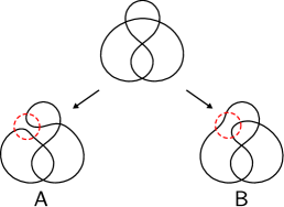
Figure 1: The states of a crossing.

Let $\displaystyle K$ be a knot diagram. If $\displaystyle m$ denotes the initial number of crossings, then the final states form a collection of $\displaystyle 2^{m}$ diagrams of nonintersecting curves. We can enumerate those states with respect to the number of their components – called circles – by introducing the sum

$$K(x):=\sum_{S}x^{|S|},$$ (1)

where $\displaystyle S$ browses the collection of states, and $\displaystyle|S|$ gives the number of circles in $\displaystyle S$. Here, $\displaystyle K(x)$ is an integer polynomial which we referred to as generating polynomial [6, 7] (in fact, it is a simplified formulation of what Kauffman calls “state polynomial” [2, Section 1–2] or “bracket polynomial” [3]). For instance, if $\displaystyle K$ is the figure-eight knot diagram, then we have $\displaystyle K(x)=5x+8x^{2}+3x^{3}$ (the states are illustrated in Figure 2).

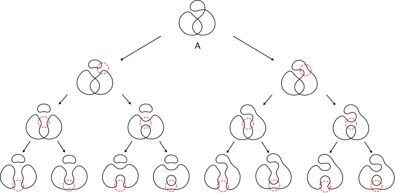
(a) The states of the figure-eight knot following the initial “$\displaystyle\mathsf{A}$” split.

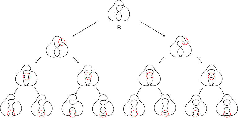
(b) The states of the figure-eight knot following the initial “$\displaystyle\mathsf{B}$” split.

Figure 2: The states of the figure-eight knot.

In this note, we establish the generating polynomial for the two-bridge knot with Conway’s notation $\displaystyle\mathcal{C}(n,r)$ [4, 5]. We refer to the associated knot diagram as $\displaystyle B_{n,r}$, where $\displaystyle n$ and $\displaystyle r$ denote the number of half-twists. For example, the figure-eight knot has Conway’s notation $\displaystyle\mathcal{C}(2,2)$. Owing to the property of the shadow diagram which we draw on the sphere [1], we can continuously deform the diagram $\displaystyle B_{n,r}$ into $\displaystyle B_{r,n}$ without altering the crossings configuration. We let $\displaystyle B_{n,r}\rightleftharpoons B_{r,n}$ express such transformation (see Figure 3 3(a)). Besides, we let $\displaystyle B_{n,0}$ and $\displaystyle B_{n,\infty}$ denote the diagrams in Figure 3 3(b) and 3(c), respectively. Here, “$\displaystyle 0$” and “$\displaystyle\infty$” are symbolic notations – borrowed from tangle theory [2, p. 88] – that express the absence of half-twists. If $\displaystyle r=\infty$ and $\displaystyle n\geq 1$, then $\displaystyle B_{n,\infty}$ represents the diagram of a $\displaystyle(2,n)$-torus knot ($\displaystyle\rightleftharpoons B_{n-1,1}$). Correspondingly, we let $\displaystyle B_{0,r}$ and $\displaystyle B_{\infty,r}$ denote the diagrams pictured in Figure 3 3(d) and 3(e), respectively.

(a) $\displaystyle B_{n,r}\rightleftharpoons B_{r,n}$.

(b) $\displaystyle B_{n,0}$.

(c) $\displaystyle B_{n,\infty}$ ($\displaystyle(2,n)$-torus knot).

(d) $\displaystyle B_{0,r}$.

(e) $\displaystyle B_{\infty,r}$ ($\displaystyle(2,r)$-torus knot).

Figure 3: Two-bridge knots with Conway’s notation $\displaystyle\mathcal{C}(n,r)$.

2 Generating polynomial

Let $\displaystyle K$, $\displaystyle K^{\prime}$ and $\displaystyle\bigcirc$ be knot diagrams, where $\displaystyle\bigcirc$ is the trivial knot, and let $\displaystyle\#$ and $\displaystyle\sqcup$ denote the connected sum and the disjoint union, respectively. The generating polynomial defined in (1) verifies the following basic properties:

1. $\displaystyle\bigcirc(x)=x$;

2. $\displaystyle\big{(}K\sqcup K^{\prime}\big{)}(x)=K(x)K^{\prime}(x)$;

3. $\displaystyle\big{(}K\#K^{\prime}\big{)}(x)=\dfrac{1}{x}K(x)K^{\prime}(x)$.

Furthermore, if $\displaystyle K\rightleftharpoons K^{\prime}$, then $\displaystyle K(x)=K^{\prime}(x)$ [6].

Lemma 1.

The generating polynomial for the knots $\displaystyle B_{n,0}$ and $\displaystyle B_{n,\infty}$ are given by

$$\displaystyle B_{n,0}(x)=x(x+1)^{n}$$ (2)

and

$$B_{n,\infty}(x)=(x+1)^{n}+x^{2}-1.$$ (3)

The key ingredient for establishing (2) and (3) consists of the states of specific crossings which produce the recurrences

$$B_{n,0}(x)=\left(\bigcirc\sqcup B_{n-1,0}\right)(x)+B_{n-1,0}(x)$$

and

$$B_{n,\infty}(x)=B_{n-1,0}(x)+B_{n-1,\infty}(x),$$

respectively, with initial values $\displaystyle B_{0,0}(x)=x$ and $\displaystyle B_{0,\infty}(x)=x^{2}$ [6]. Note that the lemma still holds if we replace index $\displaystyle n$ by $\displaystyle r$.

Proposition 2.

The generating polynomial for the two-bridge knot $\displaystyle B_{n,r}$ is given by the recurrence

$$B_{n,r}(x)=B_{n-1,r}(x)+(x+1)^{n-1}B_{\infty,r}(x),$$ (4)

and has the following closed form:

$$B_{n,r}(x)=\left(\dfrac{(x+1)^{r}+x^{2}-1}{x}\right)(x+1)^{n}+\left(x^{2}-1\right)\left(\dfrac{(x+1)^{r}-1}{x}\right).$$ (5)

Proof.

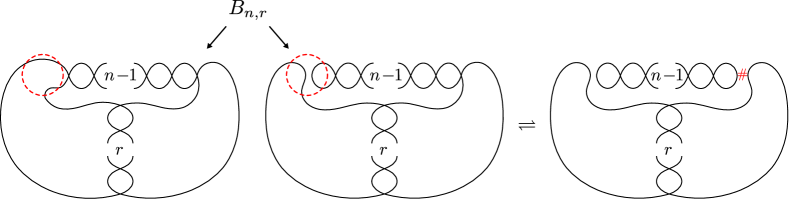
Figure 4: The splits at a crossing allow us to capture $\displaystyle B_{n-1,r}$, $\displaystyle B_{n-1,0}$ and $\displaystyle B_{\infty,r}$.

By Figure 4 we have

$$\displaystyle B_{n,r}(x) \displaystyle=B_{n-1,r}(x)+\big{(}B_{n-1,0}\#B_{\infty,r}\big{)}(x)$$

$$\displaystyle=B_{n-1,r}(x)+(x+1)^{n-1}B_{\infty,r}(x),$$

where the last relation follows from property (iii). Solving the recurrence for $\displaystyle n$ yields

$$B_{n,r}(x)=B_{0,r}(x)+B_{\infty,r}(x)\left(\dfrac{(x+1)^{n}-1}{x}\right).$$

We conclude by the closed forms in Lemma 2. ∎

Remark 3.

We can write

$$B_{n,0}(x)=x^{2}\upalpha_{n}(x)+x$$ (6)

and

$$B_{n,\infty}(x)=x\upalpha_{n}(x)+x^{2},$$ (7)

where $\displaystyle\upalpha_{n}(x):=\dfrac{(x+1)^{n}-1}{x}$, so that identity (5) becomes

$$B_{n,r}(x)=\left(x^{2}\upalpha_{n}(x)+x\right)+\left(x^{2}\upalpha_{r}(x)+x\upalpha_{n}(x)\upalpha_{r}(x)\right).$$ (8)

Since the coefficients of $\displaystyle\upalpha_{n}(x)$ are all nonnegative, it is clear, by (6), that the polynomial $\displaystyle x^{2}\upalpha_{n}(x)$ counts the states of $\displaystyle B_{n,0}$ that have at least $\displaystyle 2$ circles. This is illustrated in Figure 5 5(a). Likewise, we have an interpretation of (7) in Figure 5 5(b). In Figure 5 and 6, the dashed diagrams represent all possible disjoint union of $\displaystyle\ell-1$ circles ($\displaystyle\ell=n$ or $\displaystyle r$, depending on the context), counted by $\displaystyle\upalpha_{\ell}(x)$ and eventually empty.

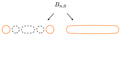
(a) Illustration of $\displaystyle x^{2}\upalpha_{n}(x)+x$.

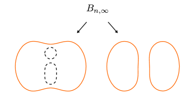
(b) Illustration of $\displaystyle x\upalpha_{n}(x)+x^{2}$.

Figure 5: Illustrations of $\displaystyle B_{n,0}(x)$ and $\displaystyle B_{n,\infty}(x)$ as functions of $\displaystyle\upalpha_{n}(x)$ .

Therefore, for $\displaystyle n,r\notin\left\{0,\infty\right\}$, identity (8) means that we can classify the states into $\displaystyle 4$ subset as shown in Figure 6. In these illustrations, there are $\displaystyle 2^{n}-1$ and $\displaystyle 2^{r}-1$ states of 6 and 6 kind, respectively, and $\displaystyle\binom{n}{1}\times\binom{r}{1}+1$ one-component states of 6 and 6 kind. The remaining states are of 6 kind, bringing the total number of states to $\displaystyle 2^{n+r}$.

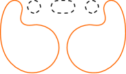
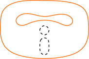
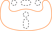
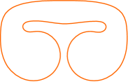
Figure 6: The states of $\displaystyle B_{n,r}$: states in 6 are counted by $\displaystyle x^{2}\upalpha_{n}(x)$, those in 6 by $\displaystyle x^{2}\upalpha_{r}(x)$, those in 6 by $\displaystyle x\upalpha_{n}(x)\upalpha_{r}(x)$, and state in 6 is simply counted by $\displaystyle x$.

3 Particular values

Let $\displaystyle\sum_{k\geq 0}b{(n,r;k)}x^{k}:=B_{n,r}(x)$, or $\displaystyle b(n,r;k):=\left[x^{k}\right]B_{n,r}(x)$. Then

$$b(n,r;k)=\binom{n+r}{k+1}+\binom{n}{k-1}+\binom{r}{k-1}-\binom{n}{k+1}-\binom{r}{k+1}-\delta_{1,k},$$

where $\displaystyle\delta_{1,k}$ is the Kronecker symbol. By (1), we recognize $\displaystyle b(n,r;k)$ as the cardinal of the set $\displaystyle\{|S|=k:S\textit{ is a state of }B_{n,r}\}$, i.e., the number of states having $\displaystyle k$ circles. In this section, the coefficients $\displaystyle b(n,r;k)$ are tabulated for some values of $\displaystyle n$, $\displaystyle r$ and $\displaystyle k$. We give as well the corresponding A-numbers in the On-Line Encyclopedia of Integer Sequences [8].

• $\displaystyle b(n,0;k)=\left[x^{k}\right]x(x+1)^{n}$, essentially giving entries in Pascal’s triangle A007318 (see Table 1).

  $\displaystyle\begin{array}[]{c|rrrrrrrrrrrrrrrrrrrrrrrrr}n\ \backslash\ k&0&1&2&3&4&5&6&7&8\\ \hline\cr 0&0&1\\ 1&0&1&1\\ 2&0&1&2&1\\ 3&0&1&3&3&1\\ 4&0&1&4&6&4&1\\ 5&0&1&5&10&10&5&1\\ 6&0&1&6&15&20&15&6&1\\ 7&0&1&7&21&35&35&21&7&1\end{array}$

  Table 1: Values of $\displaystyle b(n,0;k)$ for $\displaystyle 0\leq n\leq 7$ and $\displaystyle 0\leq k\leq 8$.

• $\displaystyle b(n,1;k)=\left[x^{k}\right]\left((x+1)^{n+1}+x^{2}-1\right)$, generating a subtriangle in A300453 (see Table 2).

  $\displaystyle\begin{array}[]{c|rrrrrrrrrrrrrrrrrrrrrrrrr}n\ \backslash\ k&0&1&2&3&4&5&6&7&8\\ \hline\cr 0&0&1&1\\ 1&0&2&2\\ 2&0&3&4&1\\ 3&0&4&7&4&1\\ 4&0&5&11&10&5&1\\ 5&0&6&16&20&15&6&1\\ 6&0&7&22&35&35&21&7&1\\ 7&0&8&29&56&70&56&28&8&1\\ \end{array}$

  Table 2: Values of $\displaystyle b(n,1;k)$ for $\displaystyle 0\leq n\leq 7$ and $\displaystyle 0\leq k\leq 8$.

• $\displaystyle b(n,2;k)=\left[x^{k}\right]\left((2x+2)(x+1)^{n}+\left(x^{2}-1\right)(x+2)\right)$, giving triangle in A300454 (see Table 3).

  $\displaystyle\begin{array}[]{c|rrrrrrrrrrrrrrrrrrrrrrrrr}n\ \backslash\ k&0&1&2&3&4&5&6&7&8\\ \hline\cr 0&0&1&2&1\\ 1&0&3&4&1\\ 2&0&5&8&3\\ 3&0&7&14&9&2\\ 4&0&9&22&21&10&2\\ 5&0&11&32&41&30&12&2\\ 6&0&13&44&71&70&42&14&2\\ 7&0&15&58&113&140&112&56&16&2\end{array}$

  Table 3: Values of $\displaystyle b(n,2;k)$ for $\displaystyle 0\leq n\leq 7$ and $\displaystyle 0\leq k\leq 8$.

• $\displaystyle b(n,n;k)=\left[x^{k}\right]\left(\dfrac{(x+1)^{2n}+\big{(}x^{2}-1\big{)}\big{(}2(x+1)^{n}-1)\big{)}}{x}\right)$, giving triangle in A321127 (see Table 4).

  $\displaystyle\begin{array}[]{c|rrrrrrrrrrrrrrrrrrrrrrrrr}n\ \backslash\ k&0&1&2&3&4&5&6&7&8&9&10&11&12&13\\ \hline\cr 0&0&1\\ 1&0&2&2\\ 2&0&5&8&3\\ 3&0&10&24&21&8&1\\ 4&0&17&56&80&64&30&8&1\\ 5&0&26&110&220&270&220&122&45&10&1\\ 6&0&37&192&495&820&952&804&497&220&66&12&1\\ 7&0&50&308&973&2030&3059&3472&3017&2004&1001&364&91&14&1\end{array}$

  Table 4: Values of $\displaystyle b(n,n;k)$ for $\displaystyle 0\leq n\leq 7$ and $\displaystyle 0\leq k\leq 13$.

• $\displaystyle b(n,r;1)=nr+1$, giving A077028, and displayed as square array in Table 5.

  $\displaystyle\begin{array}[]{c|rrrrrrrrrrrrrrrrrrrrrrrrr}n\ \backslash\ r&0&1&2&3&4&5&6&7\\ \hline\cr 0&1&1&1&1&1&1&1&1\\ 1&1&2&3&4&5&6&7&8\\ 2&1&3&5&7&9&11&13&15\\ 3&1&4&7&10&13&16&19&22\\ 4&1&5&9&13&17&21&25&29\\ 5&1&6&11&16&21&26&31&36\\ 6&1&7&13&19&25&31&37&43\\ 7&1&8&15&22&29&36&43&50\end{array}$

  Table 5: Values of $\displaystyle b(n,r;1)$ for $\displaystyle 0\leq n\leq 7$ and $\displaystyle 0\leq r\leq 7$.

  In Kauffman’s language, $\displaystyle b(n,r;1)$ is, for a fixed choice of star region, the number of ways of placing state markers at the crossings of the diagram $\displaystyle B_{n,r}$, i.e., of the forms

  $$\includegraphics[width=26.01613pt,valign={c}]{markersA1},\quad\includegraphics[angle={90},origin=c,width=26.01613pt,valign={c}]{markersA1},\quad\includegraphics[angle={180},origin=c,width=26.01613pt,valign={c}]{markersA1},\quad\includegraphics[angle={270},origin=c,width=26.01613pt,valign={c}]{markersA1},$$

  so that the resulting states are “Jordan trails” [2, Section 1–2]. Note that a state marker is interpreted as an instruction to split a crossing as shown below:

  $$\includegraphics[width=26.01613pt,valign={c}]{markersA1}\Longrightarrow\includegraphics[width=26.01613pt,valign={c}]{markersA2}\qquad\mbox{ and }\qquad\includegraphics[angle={90},origin=c,width=26.01613pt,valign={c}]{markersA1}\Longrightarrow\includegraphics[angle={90},origin=c,width=26.01613pt,valign={c}]{markersA2}.$$

  The process is illustrated in Figure 7 for the figure-eight knot.

  

  Figure 7: Illustration of $\displaystyle b(2,2;1)$: mark two adjacent regions by stars (*), then assign a state marker at each crossing so that no region of $\displaystyle B_{2,2}$ contains more than one state marker, and regions with stars do not have any.

• $\displaystyle b(n,r;2)=n\left(\binom{r}{2}+1\right)+r\left(\binom{n}{2}+1\right)$, giving square array in A300401 (see Table 6).

  $\displaystyle\begin{array}[]{c|rrrrrrrrrrrrrrrrrrrrrrrrr}n\ \backslash\ r&0&1&2&3&4&5&6&7\\ \hline\cr 0&0&1&2&3&4&5&6&7\\ 1&1&2&4&7&11&16&22&29\\ 2&2&4&8&14&22&32&44&58\\ 3&3&7&14&24&37&53&72&94\\ 4&4&11&22&37&56&79&106&137\\ 5&5&16&32&53&79&110&146&187\\ 6&6&22&44&72&106&146&192&244\\ 7&7&29&58&94&137&187&244&308\\ \end{array}$

  Table 6: Values of $\displaystyle b(n,r;2)$ for $\displaystyle 0\leq n\leq 7$ and $\displaystyle 0\leq r\leq 7$.

  We paid a special attention to the case $\displaystyle k=2$ because, surprisingly, columns $\displaystyle\big{(}b(n,1;2)\big{)}_{n}$ and $\displaystyle\big{(}b(n,2;2)\big{)}_{n}$ match sequences A000124 and A014206, respectively [6]. The former gives the maximal number of regions into which the plane is divided by $\displaystyle n$ lines, and the latter the maximal number of regions into which the plane is divided by $\displaystyle(n+1)$ circles.

• $\displaystyle b\big{(}n,r;d(n,r)\big{)}=\textit{leading coefficient of }B_{n,r}(x)$, giving square array in A321125 (see Table 7). Here, $\displaystyle d(n,r)=\max(n+1,r+1,n+r-1)$ denotes the degree of $\displaystyle B_{n,r}(x)$, and gives entries in A321126. We have Table 8 giving the numbers $\displaystyle d(n,r)$ for $\displaystyle 0\leq n\leq 7$ and $\displaystyle 0\leq r\leq 7$.

  $\displaystyle\begin{array}[]{c|rrrrrrrrrrrrrrrrrrrrrrrrr}n\ \backslash\ r&0&1&2&3&4&5&6&7\\ \hline\cr 0&1&1&1&1&1&1&1&1\\ 1&1&2&1&1&1&1&1&1\\ 2&1&1&3&2&2&2&2&1\\ 3&1&1&2&1&1&1&1&1\\ 4&1&1&2&1&1&1&1&1\\ 5&1&1&2&1&1&1&1&1\\ 6&1&1&2&1&1&1&1&1\\ 7&1&1&2&1&1&1&1&1\end{array}$

  Table 7: Leading coefficients of $\displaystyle B_{n,r}(x)$ for $\displaystyle 0\leq n\leq 7$ and $\displaystyle 0\leq r\leq 7$.

  $\displaystyle\begin{array}[]{c|rrrrrrrrrrrrrrrrrrrrrrrrr}n\ \backslash\ r&0&1&2&3&4&5&6&7\\ \hline\cr 0&1&2&3&4&5&6&7&8\\ 1&2&2&3&4&5&6&7&8\\ 2&3&3&3&4&5&6&7&8\\ 3&4&4&4&5&6&7&8&9\\ 4&5&5&5&6&7&8&9&10\\ 5&6&6&6&7&8&9&10&11\\ 6&7&7&7&8&9&10&11&12\\ 7&8&8&8&9&10&11&12&13\\ \end{array}$

  Table 8: Values of $\displaystyle d(n,r)$ for $\displaystyle 0\leq n\leq 7$ and $\displaystyle 0\leq r\leq 7$.

  We have the following properties:

  • $\displaystyle d(n,r)=d(r,n)$;

  • if $\displaystyle r=0$, then $\displaystyle d(n,r)=n+1$;

  • if $\displaystyle r=\infty$, then sequence $\displaystyle\big{(}d(n,r)\big{)}_{n}$ begins: $\displaystyle 2,2,2,3,4,5,6,7,8,\ldots$ (A233583 with offset 1).

  Diagramatically, we give the corresponding illustration for some values of $\displaystyle n$ and $\displaystyle r$ in Figure 8.

  

  (a) $\displaystyle n\geq 1$.

  

  (b) $\displaystyle n\geq 2$.

  

  (c) $\displaystyle n\geq 2$, $\displaystyle r\geq 2$.

  Figure 8: Illustration of the numbers $\displaystyle d(n,r)$.

  Correspondingly, we have

  • $\displaystyle b\big{(}n,r;d(n,r)\big{)}=b\big{(}r,n;d(r,n)\big{)}$;

  • if $\displaystyle r=0$, then $\displaystyle b\big{(}n,r;d(n,r)\big{)}=1$;

  • if $\displaystyle r=\infty$, then sequence $\displaystyle\Big{(}b\big{(}n,r;d(n,r)\big{)}\Big{)}_{n}$ begins: $\displaystyle 1,1,2,1,1,1,1,1,\ldots$ (A294619 with initial term equals to $\displaystyle 0$).

  Remarquable values in Table 7 correspond to knots $\displaystyle B_{1,1}$ (“Hopf link”, see Figure 9), $\displaystyle B_{2,2}$ (figure-eight knot, see Figure 1, 2) and $\displaystyle B_{n,2}$ (“twist knot” [6]) for $\displaystyle n\geq 3$. The latter case can be observed from identity (8) for which the leading coefficient is larger than $\displaystyle 1$ when $\displaystyle n+1=n+r-1$ is satisfied. Also, considere the identity below:

  $$B_{n,2}(x)=B_{n,0}(x)+B_{n,\infty}(x)+B_{n,\infty}(x)+\big{(}\bigcirc\sqcup B_{n,\infty}\big{)}(x).$$

  We notice that the leading coefficient is deduced from the contribution of the summands $\displaystyle B_{n,0}(x)$ and $\displaystyle\big{(}\bigcirc\sqcup B_{n,\infty}\big{)}(x)$ [6].

  

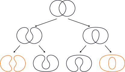
  Figure 9: The states of the knot $\displaystyle B_{1,1}$: $\displaystyle d(1,1)=2$ and $\displaystyle b\big{(}1,1,d(1,1)\big{)}=2$.

 

2010 Mathematics Subject Classification: 05A10; 57M25.

 

(Concerned with sequences A000124, A007318, A014206, A077028, A233583, A294619,
A300401, A300453, A300454, A321125, A321126 and A321127.)

References

- [1] Daniel Denton and Peter Doyle, Shadow movies not arising from knots, arXiv preprint, 2011, https://arxiv.org/abs/1106.3545.
- [2] Louis H. Kauffman, Formal Knot Theory, Princeton University Press, 1983.
- [3] Louis H. Kauffman, State models and the Jones polynomial, Topology 26 (1987), 95–107.
- [4] Kelsey Lafferty, The three-variable bracket polynomial for reduced, alternating links, Rose-Hulman Undergraduate Mathematics Journal 14 (2013), 98–113.
- [5] Matthew Overduin, The three-variable bracket polynomial for two-bridge knots, California State University REU, 2013, https://www.math.csusb.edu/reu/OverduinPaper.pdf.
- [6] Franck Ramaharo, Enumerating the states of the twist knot, arXiv preprint, 2017, https://arxiv.org/abs/1712.06543.
- [7] Franck Ramaharo, Statistics on some classes of knot shadows, arXiv preprint, 2018, https://arxiv.org/abs/1802.07701.
- [8] Neil J. A. Sloane, The On-Line Encyclopedia of Integer Sequences, published electronically at http://oeis.org, accessed 2019.