Positivity constraints on aQGC: carving out the physical parameter space

Abstract

Searching for deviations in quartic gauge boson couplings (QGCs) is one of the main goals of the electroweak program at the LHC. We consider positivity bounds adapted to the Standard Model, and show that a set of positivity constraints on 18 anomalous QGC couplings can be derived, by requiring that the vector boson scattering amplitudes of specific channels and polarisations satisfy the fundamental principles of quantum field theory. We explicitly solve the positivity inequalities to remove their dependence on the polarisations of the external particles, and obtain 19 linear inequalities, 3 quadratic inequalities, and 1 quartic inequality that only involve the QGC parameters and the weak angle. These inequalities constrain the possible directions in which deviations from the standard QGC can occur, and can be used to guide future experimental searches. We study the morphology of the positivity bounds in the parameter space, and find that the allowed parameter space is carved out by the intersection of pyramids, prisms, and (approximately) cones. Altogether, they reduce the volume of the allowed parameter space to only 2.1% of the total. We also show the bounds for some benchmark cases, where one, two, or three operators, respectively, are turned on at a time, so as to facilitate a quick comparison with the experimental results.

1 Introduction

Vector boson scattering (VBS) and triboson production processes at the LHC are among the processes most sensitive to the mechanism of electroweak symmetry breaking. In the Standard Model (SM), Feynman amplitudes involving four longitudinally polarized weak bosons individually grow with energy, but at large energy, cancellations among diagrams which involve quartic gauge boson couplings (QGC), trilinear gauge boson couplings (TGC), and Higgs exchange always occur, which lead to a total amplitude that does not grow as required by unitarity. However, effects beyond the Standard Model (BSM) could potentially spoil these cancellations and leave a trace in these channels, which can be observed at the LHC. These channels are also the unique ones to probe the QGC couplings, which are conventionally parametrised by 18 dim-8 effective operators Eboli:2006wa ; Degrande:2013rea ; Eboli:2016kko . Both ATLAS and CMS experiments have extensively searched for possible deviations in these couplings. A summary of current limits can be found in qgclimits . The most recent Run-II analyses on VBS processes, in the $W^{\pm}W^{\pm}jj$, $W^{\pm}Zjj$ and $ZZjj$ final states, have improved the precision reach on these channel ATLAS:2018ogo ; Sirunyan:2017ret ; ATLAS:2018ucv ; CMS:2018ysc ; Sirunyan:2017fvv . In particular, the CMS analyses Sirunyan:2017ret ; CMS:2018ysc ; Sirunyan:2017fvv have pushed the limits on potential BSM effects up to around TeV scale. Further improvement with future high luminosity upgrade can be expected.

Even though the QGC couplings, or the coefficients of the corresponding dim-8 operators, are free parameters from the effective field theory (EFT) point of view, to admit a UV completion they cannot simply take any values. Recently, some of the authors have shown that dim-8 QGC operator coefficients must satisfy a set of positivity bounds Zhang:2018shp . These bounds require that certain linear combinations of these operator coefficients must be positive. They are derived from the fundamental principles of quantum field theory Adams:2006sv , namely that any $VV\to VV$ scattering amplitude has to satisfy analiticity, unitarity, and Lorentz invariance. For example, from $WW\to WW$ scattering we can derive a condition of the form

$$\sum_{i}F_{i}x_{i,WW}(\vec{a},\vec{b})>0$$ (1)

where $F_{i}=F_{S,0},F_{S,1},\cdots$ are all dim-8 QGC operator coefficients, to be defined in the next section; $\vec{a},\vec{b}$ are the polarisation vectors of the two $W$ bosons being scattered, and $x_{i,WW}$ only depend on the weak angle $\theta_{W}$, and $\vec{a},\vec{b}$. For a given set of values for QGC coefficients $\{F_{i}\}$, if this condition is violated for any possible value of $\vec{a}$ and $\vec{b}$, then the $WW\to WW$ amplitude cannot be UV completed in a theory that satisfies analiticity, unitarity and Lorentz invariance, and therefore it does not make sense to study these coefficients. We will review the derivation of the positivity bounds adapted to the context of SMEFT in Section 2. Here it suffices to emphasize that the positivity bounds are very reliable bounds as their existence can be proven by simply assuming that some of the most basic properties of quantum field theory are respected in the UV.

These positivity bounds can have significant implication on experimental measurement. In Figure 1 we show the experimental constraints on two pairs of operator coefficients, from the recent CMS analysis on $WZjj$ final state, together with the corresponding positivity bounds, shown as green shaded areas. The parameter space outside of the green area violates positivity bounds, and does not correspond to any real UV model. We can see that while the measurement constrains the magnitudes of deviations from the SM, positivity bounds constrain the possible directions in which the deviations are possible at all. In the two-parameter case they carve out triangle areas in the parameter space, which reduce the physical parameter space that needs to be studied. If all QGC parameters are turned on, the total parameter space will be reduced by two orders of magnitude.

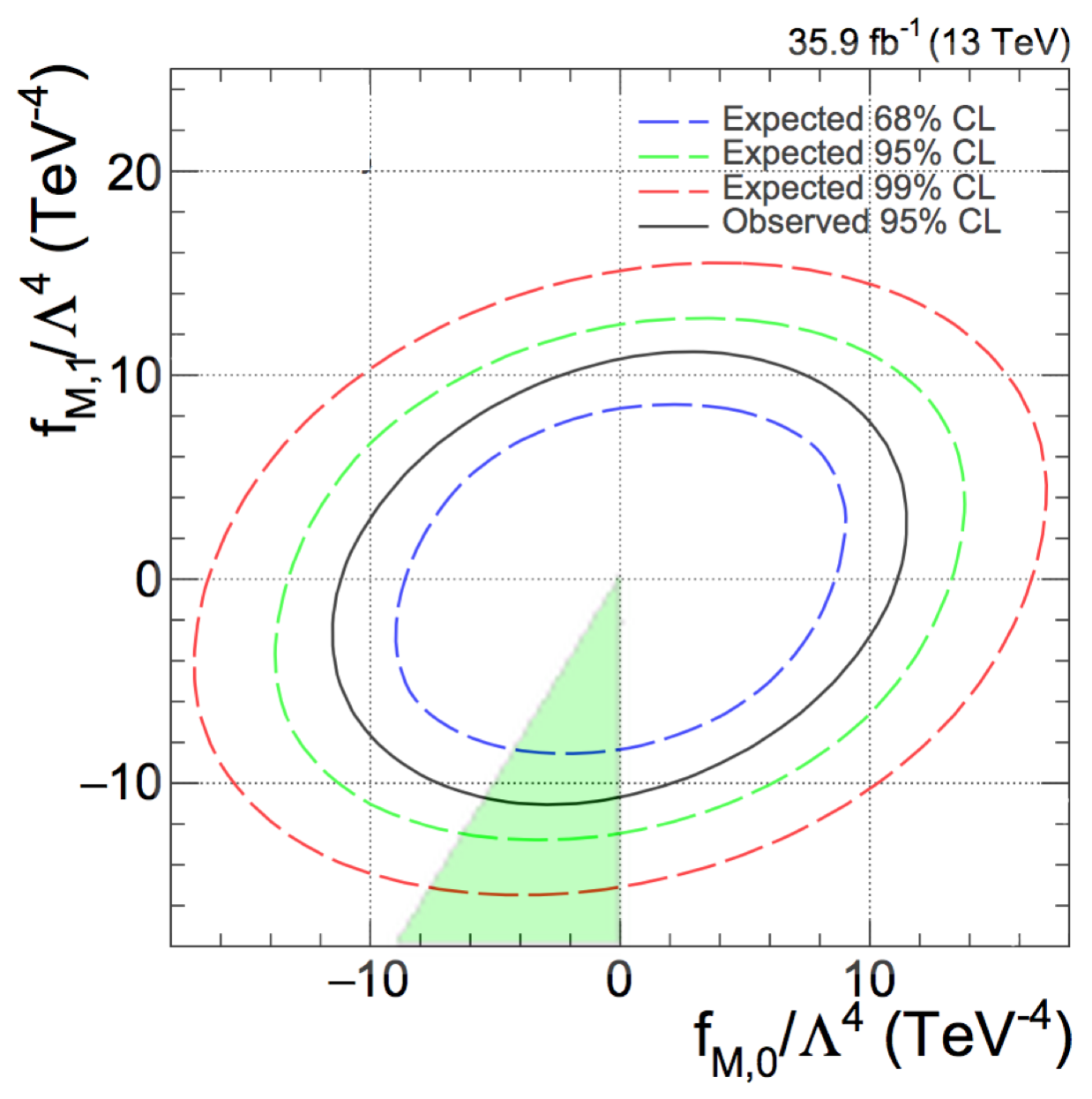
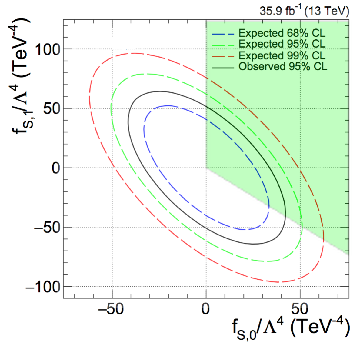
Figure 1: Limits on pairs of QGC operator coefficients from CMS $WZjj$ analysis CMS:2018ysc . Green shaded area represents positivity bounds.

These results are important in several ways. First of all, positivity constraints lead to additional physical insight of the multidimensional parameter space spanned by 18 QGC coefficients, and could provide guidance as to where one should look for deviations in QGC couplings. For example, in Figure 1 left the possible parameter space is reduced to a very narrow range, and the experimental analysis could have been focused only within this range, as BSM deviation cannot be observed elsewhere. Second, theoretical studies on QGC often follow a bottom-up approach, and in that case they are advised to keep the positivity constraints satisfied and avoid choosing unphysical benchmark parameters. Finally, as a more practical aspect, experimental limits like those in Figure 1 are often obtained by scanning the parameter space, and comparing the theory prediction at each point with the observed events. Therefore in a global SMEFT analysis where all relevant operators are taken into account, positivity constraints greatly reduce the area of parameter space that needs to be scanned, and thus improving the efficiency of experimental analysis.

In our previous work, these bounds are derived for each $VV\to VV$ amplitude, with arbitrary polarisation vectors $\vec{a}$ and $\vec{b}$. The derivation will be given in Section 2 but with more details. The resulting positivity bounds on VBS consist of 7 linear inequalities of the form $\sum_{i}F_{i}x_{i,j}(\vec{a},\vec{b})>0$, where $j=W^{\pm}W^{\pm},W^{\pm}W^{\mp},W^{\pm}Z,ZZ,W^{\pm}\gamma,Z\gamma,\gamma\gamma$ denotes the scattering channel. While this set of conditions in principle encodes all information of the bounds, they are difficult to use because the polarisation vectors $\vec{a}$ and $\vec{b}$ show up as free parameters. Each of them is a complex linear combination of three helicity states, and so in total they correspond to 12 real degrees of freedom. The positivity bounds must be satisfied not only for the basis helicities, but also for their arbitrary linear combinations. Therefore, to determine if a set of QGC coefficients $\{F_{i}\}$ are excluded by positivity conditions, one has to scan a 12-dimensional space of $\vec{a},\vec{b}$ and check if any point that violates the conditions exists. This can be done in a numerical way, but it takes time to efficiently scan a multidimensional space and is sometimes inaccurate. In Ref. Zhang:2018shp , for simplicity we have only considered real polarisation vectors. This restriction limited the constraining power of positivity bounds.

The main purpose of this work is to find the analytical form that describes exactly the allowed parameter space for all $\vec{a}$ and $\vec{b}$, by removing the polarisation dependence in positivity bounds. This is done by going through all possible complex values for $\vec{a},\vec{b}$, and combining all the corresponding bounds. We will then obtain a set of analytical inequalities independent of $\vec{a},\vec{b}$, and can be directly used in any experimental or theoretical studies. They consist of 19 linear inequalities, 3 quadratic inequalities and 1 quartic inequality. These bounds carve out higher dimensional pyramids, prisms, and cones in the parameter space spanned by the 18 QGC parameters. Their intersection gives the physically allowed parameter space. We will then discuss the shapes and volumes of these constraints. To better understand the physics origin of these constraints, we will also consider a simplified model, in which various QGC couplings can be generated by integrating out several heavy resonant states. We will show explicitly that in these models the resulting QGC couplings will naturally satisfy positivity constraints.

Finally, to help future studies on QGC couplings, we provide a number of benchmark scenarios, where we turn on only 1, 2 or 3 operators at a time. Currently experimental analyses only consider individual operators or at most operator pairs, and therefore these benchmark scenarios could provide useful information for similar analyses. It should however be kept in mind that the most useful way to identify the possible deviations from the SM is to perform global analyses, by combining different channels and turning on all QGC parameters. In that case our results are still directly applicable, and in fact the impact is stronger — we will show that the volume of the full parameter space can be reduced to about $2.1\%$.

The paper is organized as follows: in Section 2 we introduce the effective Lagrangian and the QGC operators, and adapt the positivity approach to the context of SMEFT. The resulting positivity constraints are obtained and depend on the polarisation vectors. In Section 3 we “solve” these conditions by removing the polarisation dependence, and obtain the full set of analytical inequalities that describes the allowed parameter space. We first illustrate the approach by considering two toy cases in Section 3.1, and then we solve the problem for each channel in Section 3.2. The final results are collected, further simplified, and matched to specific polarisation states in Section 3.3. These are the main results of this work. The readers who are only interested in the actual form of the positivity constraints can directly go to Eqs. (166)-(218) and Eqs. (225)-(228).

The rest of the paper is devoted to a better understanding of the constraints. In Section 4 we examine the shapes of the physical parameter space constrained by positivity bounds. In Section 5 we discuss the volume of the space allowed by various positivity conditions, which reflect their respective constraining strengths and indicate their relative importance. A collection of benchmark scenarios, where only 1, 2 or 3 operators are turned on at a time, is provided in Section 6, with exact description of the bounds in Appendices B and C. Finally, we summarise the most important results of this work in Section 7. A simplified model with explicit BSM resonances is given in Appendix A, to illustrate how positivity bounds are satisfied once these resonances are integrated out.

2 Positivity bounds

2.1 Effective operators

Let us first define the effective operators relevant in this study. The QGC couplings are parameterised in a bottom-up effective field theory (EFT) approach—the SMEFT Weinberg:1978kz ; Buchmuller:1985jz ; Leung:1984ni

$$\mathcal{L}_{\rm EFT}=\mathcal{L}_{\mathrm{SM}}+\sum_{i}\frac{f_{i}^{(6)}O_{i}^{(6)}}{\Lambda^{2}}+\sum_{i}\frac{f_{i}^{(8)}O_{i}^{(8)}}{\Lambda^{4}}+\cdots$$ (2)

Unlike the usual SMEFT truncation at the level of dim-6, a useful parametrisation of anomalous QGC requires dim-8 operators. This is mostly because the QGC couplings at dim-6 are fully correlated with 3 TGC couplings, which are better constrained by other channels such as diboson production. The dim-8 effective operators allow us to study potential QGC deviations independent of existing constraints on TGC couplings. They also parametrise the four vector vertices with arbitrary helicities of the four gauge bosons. There are additional motivations for studying these operators. Dim-6 TGC couplings $\kappa_{\gamma},\kappa_{Z},\lambda_{\gamma},\lambda_{Z}$ are only generated by loop-induced operators Elias-Miro:2013mua , so it is likely that multi-boson interactions first show up in dim-8 QGC operators which are generated at the tree level. In some strongly coupled scenarios, dim-8 QGC operators can be enhanced by more powers of BSM couplings and give larger contributions than those of the dim-6 operators, see Ref. Liu:2016idz . Also, in VBS scattering with at least one transversely polarised vector, dim-6 operators cannot interfere with the SM amplitude without any mass suppression Azatov:2016sqh , unlike dim-8 operators. Dim-6 contributions are then further suppressed by factors of $\mathcal{O}(M_{W,Z}^{2}/E^{2})$. Since the dominant sensitivity in these measurements come from the energy growing terms, dim-8 contributions are as important as dim-6 squared terms. Finally, since some of the individual limits on dim-8 QGC operators have already reached the TeV scale, demonstrating the LHC sensitivity to these higher-dimensional operators, including them allows us to make the most use of the data. We refer to Ref. Green:2016trm for a more detailed review of multi-boson interaction at the LHC.

The dim-8 QGC operators are parametrised by three types of effective operators Eboli:2006wa ; Degrande:2013rea ; Eboli:2016kko . The $S$-type operators involve only covariant derivatives of the Higgs, which correspond to the longitudinal components of the electroweak bosons. The $M$-type operators include a mix of field strengths and covariant derivatives of the Higgs, which sources both transversal and longitudinal modes. The $T$-type operators only include field strengths, and thus only give rise to transversal components. Here, we use the convention of Degrande:2013rea , which has become standard in this community. Defining

$$\hat{W}^{\mu\nu}\equiv ig\frac{\sigma^{I}}{2}W^{I,\mu\nu}\,,\qquad\hat{B}^{\mu\nu}\equiv ig^{\prime}\frac{1}{2}B^{\mu\nu}\,.$$ (3)

the 18 dimension-8 QGC operators are given by

$$\begin{aligned} \begin{array}[]{l}O_{S,0}=[(D_{\mu}\Phi)^{\dagger}D_{\nu}\Phi]\times[(D^{\mu}\Phi)^{\dagger}D^{\nu}\Phi]\\ O_{S,1}=[(D_{\mu}\Phi)^{\dagger}D^{\mu}\Phi]\times[(D_{\nu}\Phi)^{\dagger}D^{\nu}\Phi]\\ O_{S,2}=[(D_{\mu}\Phi)^{\dagger}D_{\nu}\Phi]\times[(D^{\nu}\Phi)^{\dagger}D^{\mu}\Phi]\\ O_{M,0}=\mathrm{Tr}\left[{\hat{W}_{\mu\nu}\hat{W}^{\mu\nu}}\right]\times\left[(D_{\beta}\Phi)^{\dagger}D^{\beta}\Phi\right]\\ O_{M,1}=\mathrm{Tr}\left[{\hat{W}_{\mu\nu}\hat{W}^{\nu\beta}}\right]\times\left[(D_{\beta}\Phi)^{\dagger}D^{\mu}\Phi\right]\\ O_{M,2}=\left[\hat{B}_{\mu\nu}\hat{B}^{\mu\nu}\right]\times\left[(D_{\beta}\Phi)^{\dagger}D^{\beta}\Phi\right]\\ O_{M,3}=\left[\hat{B}_{\mu\nu}\hat{B}^{\nu\beta}\right]\times\left[(D_{\beta}\Phi)^{\dagger}D^{\mu}\Phi\right]\\ O_{M,4}=\left[(D_{\mu}\Phi)^{\dagger}\hat{W}_{\beta\nu}D^{\mu}\Phi\right]\times\hat{B}^{\beta\nu}\\ O_{M,5}=\frac{1}{2}\left[(D_{\mu}\Phi)^{\dagger}\hat{W}_{\beta\nu}D^{\nu}\Phi\right]\times\hat{B}^{\beta\mu}+h.c.\\ O_{M,7}=\left[(D_{\mu}\Phi)^{\dagger}\hat{W}_{\beta\nu}\hat{W}^{\beta\mu}D^{\nu}\Phi\right]\end{array}\end{aligned}\quad\begin{aligned} \begin{array}[]{l}O_{T,0}=\mathrm{Tr}\left[{\hat{W}_{\mu\nu}\hat{W}^{\mu\nu}}\right]\times\mathrm{Tr}\left[{\hat{W}_{\alpha\beta}\hat{W}^{\alpha\beta}}\right]\\ O_{T,1}=\mathrm{Tr}\left[{\hat{W}_{\alpha\nu}\hat{W}^{\mu\beta}}\right]\times\mathrm{Tr}\left[{\hat{W}_{\mu\beta}\hat{W}^{\alpha\nu}}\right]\\ O_{T,2}=\mathrm{Tr}\left[{\hat{W}_{\alpha\mu}\hat{W}^{\mu\beta}}\right]\times\mathrm{Tr}\left[{\hat{W}_{\beta\nu}\hat{W}^{\nu\alpha}}\right]\\ O_{T,5}=\mathrm{Tr}\left[{\hat{W}_{\mu\nu}\hat{W}^{\mu\nu}}\right]\times\hat{B}_{\alpha\beta}\hat{B}^{\alpha\beta}\\ O_{T,6}=\mathrm{Tr}\left[{\hat{W}_{\alpha\nu}\hat{W}^{\mu\beta}}\right]\times\hat{B}_{\mu\beta}\hat{B}^{\alpha\nu}\\ O_{T,7}=\mathrm{Tr}\left[{\hat{W}_{\alpha\mu}\hat{W}^{\mu\beta}}\right]\times\hat{B}_{\beta\nu}\hat{B}^{\nu\alpha}\\ O_{T,8}=\hat{B}_{\mu\nu}\hat{B}^{\mu\nu}\times\hat{B}_{\alpha\beta}\hat{B}^{\alpha\beta}\\ O_{T,9}=\hat{B}_{\alpha\mu}\hat{B}^{\mu\beta}\times\hat{B}_{\beta\nu}\hat{B}^{\nu\alpha},\end{array}\end{aligned}$$ (4)

and the QGC interactions are described by

$$\mathcal{L}_{\mathrm{QGC}}=\sum_{i}\frac{f_{i}O_{i}}{\Lambda^{4}}$$ (5)

where $f_{i}$ are the corresponding coefficients of the 18 operators. Note that $O_{M,6}$ is redundant Sekulla and is not included. We have also added a Hermitian conjugate of $O_{M,5}$ in its definition Perez:2018kav . For later convenience, we redefine the coefficients as follows

$$F_{S,i}\equiv f_{S,i},\quad F_{M,i}\equiv e^{2}f_{M,i},\quad F_{T,i}\equiv e^{4}f_{T,i}.$$ (6)

By doing this, the resulting positivity constraints are free of additional couplings constants. That is, they will only involve the Weinberg angle $\theta_{W}$ and the polarisation of the vector bosons. As we will show in Section 3.3, this redefinition will not change the final form of the allowed parameter space, i.e. we can directly replace $F_{X,i}\to f_{X,i}$ in the final results.

In the following subsections, we briefly review the positivity bounds, and adapt it to the context of SMEFT.

2.2 Generic UV completion

Positivity bounds are a powerful tool to constrain the Wilson coefficients of EFTs. An EFT is a valid description of the underlying theory below a cutoff scale, beyond which the EFT needs to be UV completed, that is, replaced with a theory valid up to arbitrary high energies. As mentioned in the introduction, the existence of positivity bounds are guaranteed by some fundamental properties of S-matrix such as Lorentz invariance, unitarity, crossing symmetry, analyticity and polynomial boundedness, making them very reliable theoretical bounds. Analyticity is the statement that scattering amplitudes are analytical functions of the Mandelstam variables ($s$ and $t$) in the complex domain, apart from certain poles and branch cuts. It is tied to the concepts of causality and locality and can be proven to any order in perturbation theory. By analyticity, one can connect the UV behavior of the theory with the IR via deformation of the integration contour in the complex $s$ plane. Polynomial boundedness states that when complex momenta increase the scattering amplitudes are bounded by a certain polynomial (or for some cases a linear exponential), which is also linked to locality, arising from the fact that the amplitudes should be well defined in real space after Fourier transforms. With the help of unitarity, the more restrictive Froissart bound can be proven, which states that when $|s|\to\infty$ the amplitude $A^{q_{1}q_{2}}_{ab}(s)$ is bounded by $C_{F}s\ln^{2}s$, $C_{F}$ being a constant. These are the essential ingredients needed to derive the dispersion relations that are used to derive the positivity bounds. In this paper, we have only made use of the forward limit positivity bound, which we will review in the following, with some adaptation to the context of SMEFT.

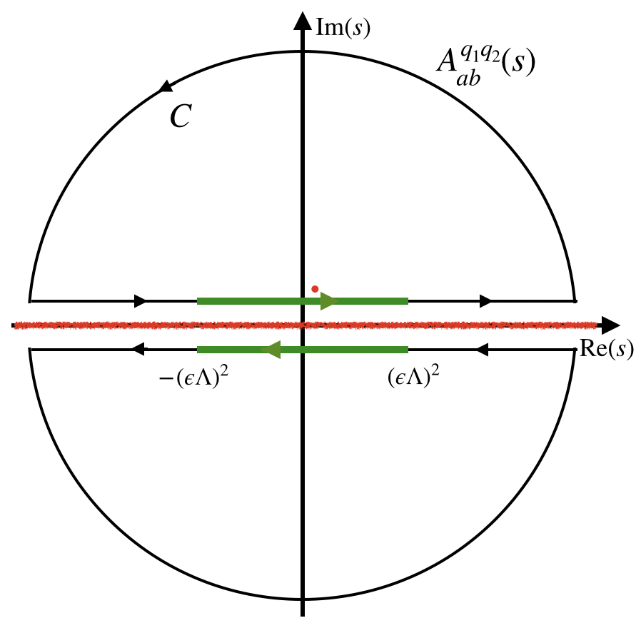
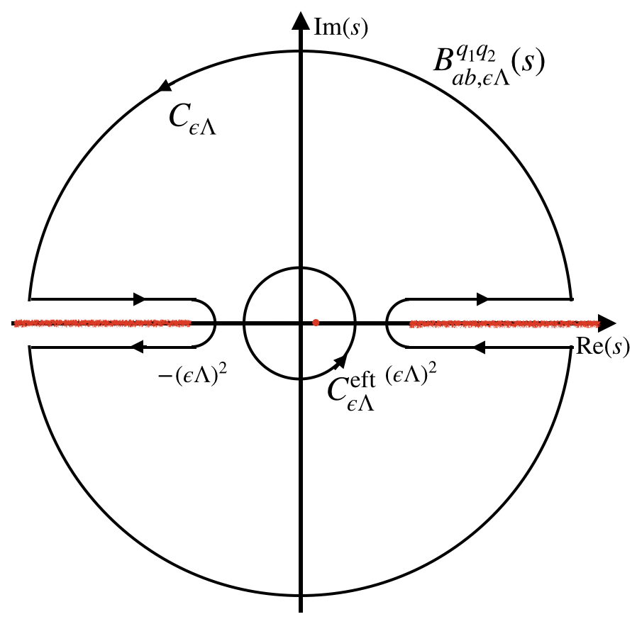
Figure 2: Dispersion relation contours in the forward limit.

Let us consider elastic scattering of two particles (ie, 2 to 2 scattering) labeled by $(m_{1},S_{1},a,q_{1})$ and $(m_{2},S_{2},b,q_{2})$, which denote the mass, spin, polarisation and remaining quantum numbers of the respective particle. For example, for $WW$ scattering $q$ is the electric charge of $W$ bosons. In the complex $s$ plane, from perturbation theory, we can infer that there are various simple poles arising from the tree level exchanges of particles and also branch cuts from internal multi-particle production at loop levels. The analyticity of the scattering amplitude requires that for fixed $t$ (we will focus on $t=0$ here: $A^{q_{1}q_{2}}_{ab}(s)=A^{q_{1}q_{2}}_{ab}(s,t=0)$) the amplitude is analytic in the complex $s$ plane apart from these singularities that already appear in perturbation theory.

In a field theory such as the SMEFT which contains massive as well as massless particles, the multi-particle productions of the massless particles give rise to branch cuts that cover the whole real axis in the $s$ plane from $-\infty$ to $+\infty$. However, below the scale $\epsilon\Lambda$ with $\epsilon\lesssim 1$, the amplitude can be computed to a desired precision in perturbation theory, so we can subtract out the simple poles and the branch cut contributions within $-(\epsilon\Lambda)^{2}<s<+(\epsilon\Lambda)^{2}$. To this end, we define the following modified amplitude deRham:2017imi ; Bellazzini:2016xrt ; deRham:2017xox

$$B^{q_{1}q_{2}}_{ab,\epsilon\Lambda}(s) \equiv A^{q_{1}q_{2}}_{ab}(s)-\frac{1}{2\pi i}\int^{+(\epsilon\Lambda)^{2}}_{-(\epsilon\Lambda)^{2}}\mathrm{d}s^{\prime}\frac{{\rm Disc}A^{q_{1}q_{2}}_{ab}(s^{\prime})}{s^{\prime}-s}$$ (7)

$$=\frac{1}{2\pi i}\oint_{\rm C}\mathrm{d}s^{\prime}\frac{A^{q_{1}q_{2}}_{ab}(s^{\prime})}{s^{\prime}-s}-\frac{1}{2\pi i}\int^{+(\epsilon\Lambda)^{2}}_{-(\epsilon\Lambda)^{2}}\mathrm{d}s^{\prime}\frac{{\rm Disc}A^{q_{1}q_{2}}_{ab}(s^{\prime})}{s^{\prime}-s}$$ (8)

$$=\frac{1}{2\pi i}\int_{\rm C^{\prime}_{\epsilon\Lambda}}\mathrm{d}s^{\prime}\frac{A^{q_{1}q_{2}}_{ab}(s^{\prime})}{s^{\prime}-s}=\frac{1}{2\pi i}\oint_{\rm C_{\epsilon\Lambda}}\mathrm{d}s^{\prime}\frac{B^{q_{1}q_{2}}_{ab,\epsilon\Lambda}(s^{\prime})}{s^{\prime}-s},$$ (9)

where the discontinuity is defined as ${\rm Disc}A^{q_{1}q_{2}}_{ab}(s^{\prime})=A^{q_{1}q_{2}}_{ab}(s^{\prime}+i\varepsilon)-A^{q_{1}q_{2}}_{ab}(s^{\prime}-i\varepsilon)$ ($\varepsilon$ being an infinitesimal positive number) and the last equality is the use of Cauchy’s integral formula for $B^{q_{1}q_{2}}_{ab,\epsilon\Lambda}(s)$. In the above, $s$ is defined away from the real axis for $A^{q_{1}q_{2}}_{ab}(s)$, but can be analytically continued to the real axis between $-\epsilon\Lambda$ and $+\epsilon\Lambda$ for $B^{q_{1}q_{2}}_{ab,\epsilon\Lambda}(s)$. As depicted in Fig 2, the left diagram is the singularity structure for $A^{q_{1}q_{2}}_{ab}(s)$ and the contour $C$ includes the upper and lower semi-circles and the full discontinuity along the real axis; the right diagram is the singularity structure for the modified amplitude $B^{q_{1}q_{2}}_{ab,\epsilon\Lambda}(s)$ and the contour $C^{\prime}_{\epsilon\Lambda}$ has the discontinuity from $-(\epsilon\Lambda)^{2}<s<+(\epsilon\Lambda)^{2}$ (the green solid contour) subtracted ($C_{\epsilon\Lambda}$ being the closed contour for $B^{q_{1}q_{2}}_{ab,\epsilon\Lambda}$). The amplitude $B^{q_{1}q_{2}}_{ab,\epsilon\Lambda}$ defined in this way has exactly the same discontinuities as $A_{ab}^{q_{1}q_{2}}$ on the real axis in $(-\infty,(\epsilon\Lambda)^{2}]\cup[(\epsilon\Lambda)^{2},+\infty)$, but the branch cuts and poles within $[-(\epsilon\Lambda)^{2},(\epsilon\Lambda)^{2}]$ are subtracted. It also has the same asymptotic behavior as $A_{ab}^{q_{1}q_{2}}$ as $s\to\infty$ and satisfies the Froissart bound. With the modified amplitude, we can define

$$f^{q_{1}q_{2}}_{ab,\epsilon\Lambda}(s) \equiv\frac{1}{2}\frac{\mathrm{d}^{2}B^{q_{1}q_{2}}_{ab,\epsilon\Lambda}(s)}{\mathrm{d}s^{2}}$$ (10)

$$=\frac{1}{2\pi i}\left(\int_{-\infty}^{-(\epsilon\Lambda)^{2}}+\int^{\infty}_{+(\epsilon\Lambda)^{2}}\right)\mathrm{d}s^{\prime}\frac{{\rm Disc}A^{q_{1}q_{2}}_{ab}(s^{\prime})}{(s^{\prime}-s)^{3}},$$ (11)

where we have used the Froissart bound and thus the infinite semi-circles parts of the contour integral vanish. Changing the integration variable for the left hand cut $s^{\prime}\to M^{2}-s^{\prime}$ ($M^{2}\equiv 2m_{1}^{2}+2m_{2}^{2}$) leads to

$$f^{q_{1}q_{2}}_{ab,\epsilon\Lambda}(s)=\frac{1}{2\pi i}\left(\int^{\infty}_{(\epsilon\Lambda)^{2}+M^{2}}\mathrm{d}s^{\prime}\frac{{\rm Disc}A^{q_{1}q_{2}}_{ab}(M^{2}-s^{\prime})}{(M^{2}-s^{\prime}-s)^{3}}+\int^{\infty}_{(\epsilon\Lambda)^{2}}\mathrm{d}s^{\prime}\frac{{\rm Disc}A^{q_{1}q_{2}}_{ab}(s^{\prime})}{(s^{\prime}-s)^{3}}\right).$$ (12)

Then we can make use of the crossing relation in the forward limit $A^{q_{1}q_{2}}_{ab}(M^{2}-s^{\prime})=A^{q_{1}\bar{q_{2}}}_{\bar{a}\bar{b}}(s^{\prime})$, where $\bar{q_{2}}$ denotes the quantum numbers of the anti-particle 2 and $\bar{a}$ and $\bar{b}$ denote possible change for the polarisations. For the discontinuity in $|s^{\prime}|>(\epsilon\Lambda)^{2}$, there is an extra minus sign:

$${\rm Disc}A^{q_{1}q_{2}}_{ab}(M^{2}-s^{\prime}) =A^{q_{1}q_{2}}_{ab}(M^{2}-s^{\prime}+i\varepsilon)-A^{q_{1}q_{2}}_{ab}(M^{2}-s^{\prime}-i\varepsilon)$$ (13)

$$=A^{q_{1}\bar{q_{2}}}_{\bar{a}\bar{b}}(s^{\prime}-i\varepsilon)-A^{q_{1}\bar{q_{2}}}_{\bar{a}\bar{b}}(s^{\prime}+i\varepsilon)=-{\rm Disc}A^{q_{1}\bar{q_{2}}}_{\bar{a}\bar{b}}(s^{\prime}).$$ (14)

Utilizing this, we get

$$f^{q_{1}q_{2}}_{ab,\epsilon\Lambda}(s)=\frac{1}{2\pi i}\left(\int^{\infty}_{(\epsilon\Lambda)^{2}+M^{2}}\mathrm{d}s^{\prime}\frac{{\rm Disc}A^{q_{1}\bar{q_{2}}}_{\bar{a}\bar{b}}(s^{\prime})}{(s^{\prime}-M^{2}+s)^{3}}+\int^{\infty}_{(\epsilon\Lambda)^{2}}\mathrm{d}s^{\prime}\frac{{\rm Disc}A^{q_{1}q_{2}}_{ab}(s^{\prime})}{(s^{\prime}-s)^{3}}\right).$$ (15)

We then convert the discontinuities of the amplitudes in the integrand to their imaginary parts via ${\rm Disc}=2i\,{\rm Im}$ and make use of the optical theorem which tells us that

$${\rm Im}A^{q_{1}q_{2}}_{ab}(s^{\prime})=\sqrt{(s^{\prime}-M_{+}^{2})(s^{\prime}-M_{-}^{2})}\sigma^{q_{1}q_{2}}_{ab}(s^{\prime})>0,~{}~{}s^{\prime}>(\epsilon\Lambda)^{2},$$ (16)

where $M_{\pm}=m_{1}\pm m_{2}$ and $\sigma^{q_{1}q_{2}}_{ab}(s^{\prime})$ is the total cross section for the $s$ channel. Similarly, we have

$${\rm Im}A^{q_{1}\bar{q_{2}}}_{\bar{a}\bar{b}}(s^{\prime})=\sqrt{(s^{\prime}-M_{+}^{2})(s^{\prime}-M_{-}^{2})}\sigma^{q_{1}\bar{q_{2}}}_{\bar{a}\bar{b}}(s^{\prime})>0,~{}~{}s^{\prime}>(\epsilon\Lambda)^{2}.$$ (17)

where $\sigma^{q_{1}\bar{q_{2}}}_{\bar{a}\bar{b}}(s^{\prime})$ is the total cross section for the $u$ channel. Putting all these together, we have

$$f^{q_{1}q_{2}}_{ab,\epsilon\Lambda}(s)>0,~{}~{}~{}~{}~{}-(\epsilon\Lambda)^{2}<s<(\epsilon\Lambda)^{2}.$$ (18)

The power of analyticity is that in the complex plane the contour $C_{\epsilon\Lambda}$ can be deformed to $C^{\rm eft}_{\epsilon\Lambda}$ which can be used to compute $f^{q_{1}q_{2}}_{ab,\epsilon\Lambda}(s)$ within the EFT framework to desired accuracy below scale $\epsilon\Lambda$.

In this work we are going to assume that the contributions from the higher dimensional operators are well approximated by the tree level, which is a reasonable assumption given that perturbativity in EFT is always required in any realistic analysis. Under this assumption $f^{q_{1}q_{2}}_{ab,\epsilon\Lambda}(s)$ can be computed as a linear combination of dim-8 coefficients plus a quadratic form of dim-6 coefficients. We will show that the latter can be removed. The SM makes no contribution at the tree level, because in the r.h.s. of Eq. (11) there are no poles nor branch points above $\epsilon\Lambda$. Its leading contribution arises at the one loop level, and could lead to small positive constant terms that weaken the positivity bound. However, in the following we will show that they are suppressed by inverse powers of $\epsilon\Lambda$, and can be safely ignored. We will also show that they can be completely removed for weakly coupled UV completion. As a result, $f^{q_{1}q_{2}}_{ab,\epsilon\Lambda}(s)>0$ directly leads to positivity constraints on Wilson coefficients.

2.3 SM loop contribution

To see that the SM contribution to $f^{q_{1}q_{2}}_{ab,\epsilon\Lambda}(s)$ is negligible, we note that the SM and EFT contributions to $f^{q_{1}q_{2}}_{ab,\epsilon\Lambda}$ are distributed differently on the real axis. While the EFT contributions stay completely above $\Lambda$, the SM contributions are dominated by the discontinuity below scale $\epsilon\Lambda$. Therefore, in the “improved positivity bounds” approach deRham:2017imi ; Bellazzini:2016xrt ; deRham:2017xox that we are using, we can choose an $\epsilon\Lambda$ to subtract the SM loop contributions as much as possible, without losing positivity. More specifically, the second term in the r.h.s. of Eq. (7) serves to subtract the SM contribution without modifying the tree level EFT contribution. The remaining SM contamination is suppressed at least by $(\epsilon\Lambda)^{-2}$. This is because the integrand in the r.h.s. of Eq. (15) goes like $s^{-3}$ for fermionic loops and $s^{-2}$ for bosonic loops.

As an example, consider the $\gamma\gamma$ scattering channel. The SM loop contribution to $f^{00}_{ab,\epsilon\Lambda}$ can be computed either by using Eq. (10) and subtracting the lower energy discontinuity, or equivalently by using the Eq. (15). The latter is more convenient because in the physical regime we can use the optical theorem, so that

$$f^{00}_{ab,\epsilon\Lambda}(0)= \frac{1}{2\pi i}\left(\int^{\infty}_{(\epsilon\Lambda)^{2}}\mathrm{d}s^{\prime}\frac{{\rm Disc}A^{00}_{\bar{a}\bar{b}}(s^{\prime})}{s^{\prime 3}}+\int^{\infty}_{(\epsilon\Lambda)^{2}}\mathrm{d}s^{\prime}\frac{{\rm Disc}A^{00}_{ab}(s^{\prime})}{s^{\prime 3}}\right)$$

$$= \frac{2}{\pi}\int^{\infty}_{(\epsilon\Lambda)^{2}}\mathrm{d}s^{\prime}\frac{1}{s^{\prime 3}}\sqrt{(s^{\prime}-M_{+}^{2})(s^{\prime}-M_{-}^{2})}\sum_{X}\sigma^{00}_{ab}(\gamma\gamma\to X)(s^{\prime}),$$ (19)

where for simplicity we have restricted to crossing symmetric amplitudes, so $A^{00}_{\bar{a}\bar{b}}=A^{00}_{ab}$. (We will see in Section 3 that, for the $\gamma\gamma$ scattering, linear polarisation gives rise to the most crucial positivity bounds.) Now $f^{00}_{ab,\epsilon\Lambda}(0)$ can be computed by evaluating the total cross sections of $\gamma\gamma\to X$, but with only the SM contributions. For one loop contribution we need to consider $\gamma\gamma\to f\bar{f}$ and $\gamma\gamma\to W^{+}W^{-}$. Since the integration is for $s>(\epsilon\Lambda)^{2}$, we take the leading contribution at large $s$. The dominant contribution comes from $\gamma\gamma\to W^{+}W^{-}$:

$$\sigma^{00}_{ab}(\gamma\gamma\to W^{+}W^{-})(s)=\frac{8\pi\alpha^{2}}{m_{W}^{2}}\left[\left(a_{1}^{2}+a_{2}^{2}\right)\left(b_{1}^{2}+b_{2}^{2}\right)\right]+\mathcal{O}(s^{-1})$$ (20)

where $a_{1,2}$ and $b_{1,2}$ are the transversal polarisation components of the two photons. This gives rise to an $\mathcal{O}\left[(\epsilon\Lambda)^{-2}\right]$ contribution to $f^{00}_{ab,\epsilon\Lambda}(0)$:

$$f^{00,WW}_{ab,\epsilon\Lambda}(0)=\frac{16\alpha^{2}}{(\epsilon\Lambda)^{2}m_{W}^{2}}\left[\left(a_{1}^{2}+a_{2}^{2}\right)\left(b_{1}^{2}+b_{2}^{2}\right)\right]+\mathcal{O}\left[(\epsilon\Lambda)^{-4}\right]$$ (21)

The $1/m_{W}^{2}$ factor is from the $t$- and $u$-channel $W$-boson propagators. The cross section of $\gamma\gamma\to f\bar{f}$ does not have this behavior and is suppressed by one extra power of $s$:

$$\sigma^{00}_{ab}(\gamma\gamma\to f\bar{f})(s)=N_{c}Q^{4}\frac{4\pi\alpha^{2}}{s}\left[\left(a_{1}^{2}+a_{2}^{2}\right)\left(b_{1}^{2}+b_{2}^{2}\right)\log\frac{s}{m_{f}^{2}}-2(a_{1}b_{1}-a_{2}b_{2})^{2}\right]+\mathcal{O}(s^{-2})$$ (22)

which gives rise to an $\mathcal{O}\left[(\epsilon\Lambda)^{-4}\right]$ contribution to $f^{00}_{ab,\epsilon\Lambda}(0)$:

$$f^{00,ff}_{ab,\epsilon\Lambda}(0)= N_{c}Q^{4}\frac{2\alpha^{2}}{(\epsilon\Lambda)^{4}}\left[2\left(a_{1}^{2}+a_{2}^{2}\right)\left(b_{1}^{2}+b_{2}^{2}\right)\log\frac{(\epsilon\Lambda)^{2}}{m_{f}^{2}}+(a_{1}^{2}+a_{2}^{2})(b_{1}^{2}+b_{2}^{2})-4(a_{1}b_{1}-a_{2}b_{2})^{2}\right]$$

$$+\mathcal{O}\left[(\epsilon\Lambda)^{-6}\right]$$ (23)

Now we can estimate the size of the SM loop contamination. The most constraining experimental limits come from scattering of high mass $VV$ pairs, up to $1.5\sim 2$ TeV CMS:2018ysc ; Sirunyan:2017fvv , so we have to assume that the EFT is well-behaved within this range, and take $\epsilon\Lambda=2$ TeV. Note that a large $\epsilon\Lambda$ does not affect the EFT contribution: at the tree level there is no branch cut below $\Lambda$, while loop corrections in EFT are always further suppressed by additional loop factors. With this value the SM loop contribution is completely dominated by $\gamma\gamma\to WW$. We find

$$f^{00,WW}_{\epsilon\Lambda}=0.038\ \mathrm{TeV}^{-4}$$ (24)

for both the $a\parallel b$ and $a\perp b$ cases.

This contribution is much smaller than a typical EFT contribution. The current limits on $f_{i}$ span several orders of magnitude qgclimits , but even the tightest ones are around $\mathcal{O}(1)(\Lambda/\mathrm{TeV})^{4}$. This is in a slightly different set of conventions by Refs. Eboli:2006wa ; Eboli:2016kko , whose coefficients will be denoted with superscript EGM in the following. Taking into account the relation between the two sets of conventions, a typical EFT contribution to $f^{00}_{\epsilon\Lambda}$ is simply of order $f_{i}^{EGM}/\Lambda^{4}$, meaning that each operator is expected to contribute about $\mathcal{O}(1)$ TeV^-4, much larger than Eq. (24). In practice the these contributions could vary by numerical factors. For example, we find that the contribution from $f_{T,7}^{EGM}$ in the $a\parallel b$ case is

$$4s_{W}^{2}c_{W}^{2}\frac{F_{T,7}^{EGM}}{\Lambda^{4}}=0.69\ \mathrm{TeV}^{-4}\frac{F_{T,7}^{EGM}\mathrm{TeV}^{4}}{\Lambda^{4}}$$ (25)

which is still more than one order of magnitude larger than the SM loops. $F_{T,8}^{EGM}$ gives a much larger contribution, which is $9.7\ \mathrm{TeV}^{-4}$, while the smallest contribution is from $F_{T,2}^{EGM}$, which gives $0.1\ \mathrm{TeV}^{-4}$. In any case, we see that the SM loop contribution cannot qualitatively affect the positivity bounds.

If future experimental sensitivity could improve significantly, it is possible that the SM contribution should be taken into account as a constant correction in $f^{00}_{ab,\epsilon\Lambda}(0)$. Its size is not difficult to compute as we have shown in the $\gamma\gamma$ case. However, in the next subsection we will show that if the UV completion is weakly coupled, this SM contribution can be completely removed, without leaving any impact on the positivity condition.

2.4 Weakly coupled UV completion

The standard Wilsonian UV completion usually postulates the existence of extra weak couplings beyond the SM, which can be used to order the loop expansion, and the leading UV amplitude already satisfies the required properties (particularly the Froissart bound) that are needed to derive the dispersion relation. In this case we can derive positivity for the specific BSM amplitude at the leading tree or loop order, and the results are free of contaminations from the SM.

If the BSM amplitude arises at the tree level by one heavy particle exchange between two SM vector boson currents, we can simply derive the positivity bound for the tree level amplitude $A^{q_{1}q_{2}}_{ab,{\rm tr}}$ as follows

$$f^{q_{1}q_{2}}_{ab,{\rm tr}}(s) \equiv\frac{1}{2}\frac{\mathrm{d}^{2}B^{q_{1}q_{2}}_{ab,{\rm tr}}(s)}{\mathrm{d}s^{2}}$$ (26)

$$=\frac{1}{2\pi i}\left(\int_{-\infty}^{-\Lambda_{\rm th}^{2}}+\int^{\infty}_{+\Lambda_{\rm th}^{2}}\right)\mathrm{d}s^{\prime}\frac{{\rm Disc}A^{q_{1}q_{2}}_{ab,{\rm tr}}(s^{\prime})}{(s^{\prime}-s)^{3}},$$ (27)

where $B^{q_{1}q_{2}}_{ab,{\rm tr}}(s)$ is the tree level amplitude with the lower energy poles subtracted from $A^{q_{1}q_{2}}_{ab,{\rm tr}}$, and $\Lambda_{\rm th}$ is the energy scale of the lowest massive state that lies beyond the EFT cutoff; see Fig 3. All the mass poles that lie above $\Lambda$ will contribute to the discontinuity from $-\infty$ to $-\Lambda_{\rm th}^{2}$ and from $\Lambda_{\rm th}^{2}$ to $+\infty$. (The tree level poles contribute to the imaginary part thanks to the Feynman $i\varepsilon$.) Similar to the previous subsection, we can obtain

$$f^{q_{1}q_{2}}_{ab,{\rm tr}}(s)=\int^{\infty}_{\Lambda_{\rm th}^{2}+M^{2}}\mathrm{d}s^{\prime}\frac{{\rm Im}A^{q_{1}\bar{q_{2}}}_{\bar{a}\bar{b},{\rm tr}}(s^{\prime})}{(s^{\prime}-M^{2}+s)^{3}}+\int^{\infty}_{\Lambda_{\rm th}^{2}}\mathrm{d}s^{\prime}\frac{{\rm Im}A^{q_{1}q_{2}}_{ab,{\rm tr}}(s^{\prime})}{(s^{\prime}-s)^{3}}.$$ (28)

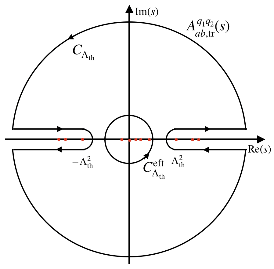
Figure 3: Tree level dispersion relation contour in the forward limit.

At the tree level, the contributions to ${\rm Im}A^{q_{1}q_{2}}_{ab,{\rm tr}}$ comes from diagrams with a heavy particle propagator $X$. By the cutting rules, ${\rm Im}A^{q_{1}q_{2}}_{ab,{\rm tr}}$ can be written as a positive sum of complete squares of the two-to-$X$ amplitudes, meaning ${\rm Im}A^{q_{1}q_{2}}_{ab,{\rm tr}}(s^{\prime})>0$ and similarly ${\rm Im}A^{q_{1}\bar{q_{2}}}_{\bar{a}\bar{b},{\rm tr}}(s^{\prime})>0$ for $s^{\prime}>\Lambda_{\rm th}^{2}$. This leads to the leading tree level positivity bound

$$f^{q_{1}q_{2}}_{ab,{\rm tr}}(s)>0,~{}~{}~{}~{}~{}-\Lambda_{\rm th}^{2}<s<\Lambda_{\rm th}^{2}.$$ (29)

without any possible contribution from the SM.

Figure 4: Examples of BSM contribution arising from heavy particle loops. Double lines represent BSM particles.

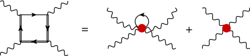
Figure 5: If the leading BSM loop contribution contains SM fields in the loop, the diagram needs to be matched to both tree-level and loop-level diagrams in the EFT. Red blobs represent higher-dimensional vertices.

More generally, the leading BSM contribution in VBS may arise from loop diagrams. For example, the EFT operator may come from integrating out heavy particle loops in diagrams shown in Figure 4. Only BSM particles can run in the loop, otherwise the contribution needs to be matched to both tree level and loop level EFT diagrams, contradicting with our initial assumption that the higher dimensional contributions are well approximated by the tree level. An example is shown in Figure 5, where the operator that enters at the tree level is loop-induced, while the one enters at the loop level is generated by a tree level graph. If all loop particles are heavy, we can simply consider the leading BSM loop contributions, which also satisfies the required properties to derive positivity. More specifically, we define

$$f^{q_{1}q_{2}}_{ab,{\rm lp}}(s)\equiv\frac{1}{2}\frac{\mathrm{d}^{2}B^{q_{1}q_{2}}_{ab,{\rm lp}}(s)}{\mathrm{d}s^{2}}=\int^{\infty}_{\Lambda_{\rm th}^{2}+M^{2}}\mathrm{d}s^{\prime}\frac{{\rm Im}A^{q_{1}\bar{q_{2}}}_{\bar{a}\bar{b},{\rm lp}}(s^{\prime})}{(s^{\prime}-M^{2}+s)^{3}}+\int^{\infty}_{\Lambda_{\rm th}^{2}}\mathrm{d}s^{\prime}\frac{{\rm Im}A^{q_{1}q_{2}}_{ab,{\rm lp}}(s^{\prime})}{(s^{\prime}-s)^{3}}.$$ (30)

where we consider the leading BSM loop contributions to the discontinuity of the amplitudes, which arise at $n$-loop, and now $\Lambda_{\rm th}$ is the threshold for multi-particle production of the BSM states. By using cutting rules, again ${\rm Im}A^{q_{1}q_{2}}_{ab,{\rm lp}}(s^{\prime})$ and ${\rm Im}A^{q_{1}\bar{q_{2}}}_{\bar{a}\bar{b},{\rm lp}}(s^{\prime})$ can be written as a sum of products of two 2-to-$X$ amplitudes at $s^{\prime}>\Lambda_{\rm th}^{2}$, where $X$ is a $n+1$ heavy particle final state. The two amplitudes in each product must be the same order, otherwise BSM loop contribution could have arose from a lower order, so each product must be a complete square, and thus

$$f^{q_{1}q_{2}}_{ab,{\rm lp}}(s)>0,~{}~{}~{}~{}~{}-\Lambda_{\rm th}^{2}<s<\Lambda_{\rm th}^{2}.$$ (31)

To sum up, if the UV completion is weakly coupled, we can derive the positivity bounds for the leading order (which may be the tree level or any loop order) BSM contributions to VBS, and the results are not affected by any SM loop contaminations. This means the resulting positivity bounds will continue to be relevant, no matter how much the experimental precision will improve in the future.

2.5 Results

Now we are ready to apply the positivity condition $f^{q_{1}q_{2}}_{ab}>0$ to VBS and set constraints on QGC operators. To this end, consider the two-by-two scattering of the SM electroweak gauge boson fields

$$V_{1}V_{2}\to V_{1}V_{2},~{}~{}~{}~{}~{}~{}V_{i}=Z,W^{\pm},\gamma,$$ (32)

with the polarisation vectors

$$\epsilon^{\mu}(V_{1}) =\sum_{i=1}^{3}a_{i}\epsilon^{\mu}_{(i)}=\left(a_{3}\frac{p_{1}}{m_{V_{1}}},a_{1},a_{2},a_{3}\frac{E_{1}}{m_{V_{1}}}\right),$$ (33)

$$\epsilon^{\mu}(V_{2}) =\sum_{i=1}^{3}b_{i}\epsilon^{\mu}_{(i)}=\left(b_{3}\frac{p_{2}}{m_{V_{2}}},b_{1},b_{2},b_{3}\frac{E_{2}}{m_{V_{2}}}\right),$$ (34)

where the linear polarisation basis is given by

$$\epsilon^{\mu}_{(1)}(V)=(0,1,0,0),~{}~{}~{}\epsilon^{\mu}_{(2)}(V)=(0,0,1,0),~{}~{}~{}\epsilon^{\mu}_{(3)}(V)=\frac{1}{m_{V}}(p_{V},0,0,E_{V}),$$ (35)

and $a_{i}$, $b_{i}$ are arbitrary complex numbers (with non-vanishing $a_{3}$, $b_{3}$ only for massive vectors). We will use $\vec{a}\equiv(a_{1},a_{2},a_{3})$ and $\vec{b}\equiv(b_{1},b_{2},b_{3})$ to denote the polarisation state. The amplitude can be computed at the tree level using standard tools Alloul:2013bka ; Hahn:2000kx ; Hahn:1998yk . We find that $f^{q_{1}q_{2}}_{ab}>0$ for all 7 $VV\to VV$ channels leads to the following conditions:

$$ZZ:$$

$$8A_{1}(4(2F_{T,0}+2F_{T,1}+F_{T,2})c_{W}^{8}+2(2F_{T,5}+2F_{T,6}+F_{T,7})c_{W}^{4}s_{W}^{4}+(2F_{T,8}+F_{T,9})s_{W}^{8})$$

$$+4A_{2}(4F_{T,2}c_{W}^{8}+2F_{T,7}c_{W}^{4}s_{W}^{4}+F_{T,9}s_{W}^{8})+(A_{3}+A^{\prime}_{3})((-4F_{M,1}+2F_{M,7})c_{W}^{6}+2F_{M,5}c_{W}^{4}s_{W}^{2}-2F_{M,3}c_{W}^{2}s_{W}^{4})$$

$$+(A_{4}+A^{\prime}_{4})(8(4F_{T,0}+4F_{T,1}+F_{T,2})c_{W}^{8}+4(4F_{T,5}+4F_{T,6}+F_{T,7})c_{W}^{4}s_{W}^{4}+2(4F_{T,8}+F_{T,9})s_{W}^{8})$$

$$+(A_{5}+A^{\prime}_{5})((8F_{M,0}-2F_{M,1}+F_{M,7})c_{W}^{6}+(4F_{M,4}+F_{M,5})c_{W}^{4}s_{W}^{2}+(4F_{M,2}-F_{M,3})c_{W}^{2}s_{W}^{4})$$

$$+16A_{6}(F_{S,0}+F_{S,1}+F_{S,2})c_{W}^{4}>0$$ (36)

$$W^{\pm}W^{\pm}:$$

$$2A_{1}(8F_{T,0}+12F_{T,1}+5F_{T,2})+6A_{2}F_{T,2}+(A_{3}+A_{3}^{\prime})(-2F_{M,1}+F_{M,7})$$

$$+2A_{4}(8F_{T,1}+F_{T,2})+2A_{4}^{\prime}(8F_{T,0}+4F_{T,1}+F_{T,2})+A^{\prime}_{5}(4F_{M,0}-F_{M,1}+F_{M,7})$$

$$+4A_{6}(2F_{S,0}+F_{S,1}+F_{S,2})>0$$ (37)

$$W^{\pm}W^{\mp}:$$

$$2A_{1}(8F_{T,0}+12F_{T,1}+5F_{T,2})+6A_{2}F_{T,2}+(A_{3}+A_{3}^{\prime})(-2F_{M,1}+F_{M,7})$$

$$+2A^{\prime}_{4}(8F_{T,1}+F_{T,2})+2A_{4}(8F_{T,0}+4F_{T,1}+F_{T,2})+A_{5}(4F_{M,0}-F_{M,1}+F_{M,7})$$

$$+4A_{6}(2F_{S,0}+F_{S,1}+F_{S,2})>0$$ (38)

$$W^{\pm}Z:$$

$$4A_{1}(4(4F_{T,1}+F_{T,2})c_{W}^{5}+(4F_{T,6}+F_{T,7})c_{W}s_{W}^{4})+4A_{2}c_{W}(4F_{T,2}c_{W}^{4}+F_{T,7}s_{W}^{4})$$

$$-4A_{3}((2F_{M,1}-F_{M,7})c_{W}^{5}+F_{M,5}c_{W}^{3}s_{W}^{2}+F_{M,3}c_{W}s_{W}^{4})$$

$$+4A_{3}^{\prime}(-2F_{M,1}+F_{M,7})c_{W}^{3}+8(A_{4}+A_{4}^{\prime})c_{W}(4F_{T,1}c_{W}^{4}+F_{T,6}s_{W}^{4})$$

$$+(A_{5}+A_{5}^{\prime})(2F_{M,7}c_{W}^{4}+F_{M,5}s_{W}^{2}+4F_{M,4}c_{W}^{2}s_{W}^{2}-F_{M,5}s_{W}^{4})$$

$$+16A_{6}(F_{S,0}+F_{S,2})c_{W}^{3}>0$$ (39)

$$Z\gamma:$$

$$A_{1}(F_{T,7}+16(2F_{T,0}+2F_{T,1}+F_{T,2})c_{W}^{4}-8F_{T,7}s_{W}^{2}-16F_{T,5}c_{W}^{2}s_{W}^{2}+8F_{T,7}s_{W}^{4}+8F_{T,8}s_{W}^{4}$$

$$+4F_{T,9}s_{W}^{4}+4F_{T,6}(1-2s_{W}^{2})^{2})+A_{2}(8F_{T,2}c_{W}^{4}+2F_{T,9}s_{W}^{4}+F_{T,7}(1-2s_{W}^{2})^{2})$$

$$+(A_{3}+A_{3}^{\prime})(4(4F_{T,0}+4F_{T,1}+F_{T,2})c_{W}^{4}-2(4F_{T,5}+F_{T,7})c_{W}^{2}s_{W}^{2}+(4F_{T,8}+F_{T,9})s_{W}^{4}+2F_{T,6}(1-2s_{W}^{2})^{2})$$

$$+A^{\prime\prime}_{3}(F_{M,7}-(2F_{M,1}+F_{M,3}+F_{M,5})c_{W}^{2}-F_{M,7}s_{W}^{2})>0$$ (40)

$$W^{\pm}\gamma:$$

$$A_{1}(16F_{T,1}+4F_{T,2}+4F_{T,6}+F_{T,7})+A_{2}(4F_{T,2}+F_{T,7})+A_{3}(-2F_{M,1}-F_{M,3}+F_{M,5}+F_{M,7})$$ (41)

$$+2(A_{4}+A^{\prime}_{4})(4F_{T,1}+F_{T,6})>0$$ (42)

$$\gamma\gamma:$$

$$4A_{1}(8F_{T,0}+8F_{T,1}+4F_{T,2}+4F_{T,5}+4F_{T,6}+2F_{T,7}+2F_{T,8}+F_{T,9})+2A_{2}(4F_{T,2}+2F_{T,7}+F_{T,9})$$

$$(A_{4}+A^{\prime}_{4})(16F_{T,0}+16F_{T,1}+4F_{T,2}+8F_{T,5}+8F_{T,6}+2F_{T,7}+4F_{T,8}+F_{T,9})>0$$ (43)

where the arbitrary complex parameters $a_{i}$ and $b_{i}$ form the following combinations

$$\begin{aligned} &A_{1}\equiv|a_{1}|^{2}|b_{1}|^{2}+|a_{2}|^{2}|b_{2}|^{2},\\ &A_{2}\equiv|a_{1}|^{2}|b_{2}|^{2}+|a_{2}|^{2}|b_{1}|^{2},\\ &A_{3}\equiv(|b_{1}|^{2}+|b_{2}|^{2})|a_{3}|^{2},\\ &A^{\prime}_{3}\equiv(|a_{1}|^{2}+|a_{2}|^{2})|b_{3}|^{2},\\ &A^{\prime\prime}_{3}\equiv|b_{1}|^{2}|a_{3}|^{2}\end{aligned}\qquad~{}~{}\begin{aligned} &A_{4}\equiv a_{1}a_{2}^{*}b_{1}b_{2}^{*}+c.c.,\\ &A^{\prime}_{4}\equiv a_{1}a_{2}^{*}b_{1}^{*}b_{2}+c.c.,\\ &A_{5}\equiv(a_{1}b_{1}+a_{2}b_{2})a_{3}^{*}b_{3}^{*}+c.c.,\\ &A^{\prime}_{5}\equiv-(a_{1}b_{1}^{*}+a_{2}b_{2}^{*})a_{3}^{*}b_{3}+c.c.\\ &A_{6}\equiv|a_{3}|^{2}|b_{3}|^{2},\end{aligned}$$ (44)

and we have also defined

$$s_{W}\equiv\sin\theta_{W},\quad c_{W}\equiv\cos\theta_{W},\quad t_{W}\equiv\tan\theta_{W},~{}~{}~{}~{}~{}\theta_{W}\text{~{}being weak angle}.$$ (45)

In Section 3.2 we will see that the $W^{\pm}W^{\pm}$ channel and the $W^{\pm}W^{\mp}$ channel give equivalent bounds. For the rest of the paper we will only consider $W^{\pm}W^{\pm}$, and omit the superscript $\pm$.

We have neglected the contribution from dim-6 operators. In Ref. Zhang:2018shp we have shown by explicit calculations that their contributions to the l.h.s. of the inequalities are always negative-definite, which means that dropping these terms will only make the positivity conditions more conservative. For completeness, here we give these contributions in the Warsaw basis Grzadkowski:2010es , but for the rest of the paper we will drop them. They read

$$WZ:$$

$$-a_{3}^{2}b_{3}^{2}s_{W}^{4}c_{W}^{2}\left(c_{W}C_{\varphi D}+4s_{W}C_{\varphi WB}\right)^{2}-36(a_{1}b_{1}+a_{2}b_{2})^{2}e^{2}s_{W}^{2}c_{W}^{2}C_{W}^{2}+\mbox{dim-8 terms}>0$$ (46)

$$WW:$$

$$-a_{3}^{2}b_{3}^{2}s_{W}^{2}c_{W}^{4}C_{\varphi D}^{2}-36(a_{1}b_{1}+a_{2}b_{2})^{2}e^{2}s_{W}^{2}c_{W}^{2}C_{W}^{2}+\mbox{dim-8 terms}>0$$ (47)

$$W\gamma:$$

$$-(a_{1}b_{1}+a_{2}b_{2})^{2}C_{W}^{2}+\mbox{dim-8 terms}>0$$ (48)

and there are no contribution in the other four channels.

We could have considered amplitudes that involve the Higgs boson, such as $VH\to VH$, to derive more bounds. However, the dim-8 parametrisation of QGC has only included the relevant operators that involve four-gauge-boson vertices and are independent of TGCs. In principle, other operators might also enter the $VH\to VH$ vertex, and this will lead to results that depend on non-QGC operators. For this reason we have focused on the VBS channels, where all relevant operators are included in the QGC parameterisation.

In our previous work Zhang:2018shp , for computational simplicity we have restricted ourselves to positivity bounds for real $a_{i}$ and $b_{i}$ corresponding to crossing symmetric amplitudes with linear polarisations. In this work we will consider arbitrary complex polarisations. We will see that even though the vast majority of the constraining power comes from real polarisations, including complex polarisations does bring improvements, which could be significant if only one or several operators are turned on.

3 Solving the positivity conditions

The positivity conditions given in the previous section can be schematically written as

$$\sum_{i}F_{i}x_{i,j}(\vec{a},\vec{b})>0$$ (49)

where $F_{i}$ are all coefficients, $j$ denotes the scattering channel, and the $x_{i}$’s are complex quartic homogeneous polynomial functions of $a_{i}$ and $b_{i}$. These conditions needs to be satisfied for arbitrary values of the polarisation vectors $\vec{a}$ and $\vec{b}$. As we have mentioned, these conditions are inconvenient because they involve $\vec{a}$ and $\vec{b}$ as free parameters. The goal of this section is to solve these inequalities and remove the $\vec{a}$ and $\vec{b}$ dependence. This is done by going through all possible complex values for $\vec{a},\vec{b}$, which span a 6-dimensional complex space, obtaining the bounds for each polarisation, and combining all the resulting bounds. By doing this, we will obtain the simplest description for the physical parameter space that is independent of any free parameters, which can be used directly in future experimental as well as theoretical studies.

3.1 Toy cases

Before solving the positivity conditions in the most general case, it is illustrative to consider some toy cases, to explain our approach and to develop physics intuition.

3.1.1 The pyramid case

Let us consider a case where we only allow three operator coefficients, $F_{M,0}$, $F_{M,1}$ and $F_{M,5}$ to be nonzero. We also restrict $\vec{a}$ and $\vec{b}$ to take real values only. The problem is reduced to a 3-dimensional one. We can write the positivity conditions in the form of the inner product of two vectors:

$$\vec{F}\cdot\vec{x}_{i}(\vec{a},\vec{b})>0$$ (50)

where $\vec{F}=(F_{M,0},F_{M,1},F_{M,5})$ is a coefficient vector, and $i=WW,WZ,\cdots$ are different channels. The $\vec{x}_{i}$ vectors are:

$$\vec{x}_{WW}=\left(-4T_{a}T_{b}\cos\phi,-T_{a}^{2}+T_{a}T_{b}\cos\phi-T_{b}^{2},0\right)$$ (51)

$$\vec{x}_{ZZ}=(0,-2c_{W}^{2},s_{W}^{2})$$ (52)

$$\vec{x}_{WZ}=\left(0,-2c_{W}^{2}T_{a}^{2}-2T_{b}^{2},-s_{W}^{2}T_{a}^{2}\right)$$ (53)

$$\vec{x}_{W\gamma}=(0,-2,1)$$ (54)

$$\vec{x}_{Z\gamma}=(0,-2,-1)$$ (55)

and $\vec{x}_{\gamma\gamma}$ does not give any nontrivial condition. Here $T_{a}$, $T_{b}$, and $\cos\phi$ are defined as

$$T_{a}=\frac{a_{3}}{\sqrt{a_{1}^{2}+a_{2}^{2}}},\quad T_{b}=\frac{b_{3}}{\sqrt{b_{1}^{2}+b_{2}^{2}}}\,.$$ (56)

$$\cos\phi=\frac{a_{1}b_{1}+a_{2}b_{2}}{\sqrt{a_{1}^{2}+a_{2}^{2}}\sqrt{b_{1}^{2}+b_{2}^{2}}}$$ (57)

Positivity conditions simply state that the coefficients, $\vec{F}$, must be positive once projected onto any of the $\vec{x}_{i}(\vec{a},\vec{b})$ vectors.

The set of vectors $X=\{\vec{x}_{i}(\vec{a},\vec{b})\}$ encodes all the information to describe the actual bounds. The problem now is to identify the simplest way to describe this vector set, or one that gives exactly the same bounds, without referring to the polarisation vector $\vec{a},\vec{b}$. A useful fact is the following: if a specific vector $\vec{x}$ can be written as a positive linear combination of some other vectors in the set, specified by channel $i$ and polarisation $\vec{a}_{j},\vec{b}_{j}$, i.e.

$$\vec{x}=\sum_{i,j}c_{i,j}\vec{x_{i}}(\vec{a}_{j},\vec{b}_{j}),\quad c_{i,j}\geq 0$$ (58)

then this vector $\vec{x}$ can be removed form the set $X$, without affecting the allowed parameter space. This is because

$$\vec{F}\cdot\vec{x}=\sum_{i,j}c_{i,j}\vec{F}\cdot\vec{x_{i}}(\vec{a}_{j},\vec{b}_{j})$$ (59)

but each term on the r.h.s is already positive, so $\vec{F}\cdot\vec{x}>0$ does not lead to new exclusion. Making use of this, we can keep removing redundant $\vec{x}$ vectors from the set $X$, until it reaches the simplest form.

More specifically, we proceed as follows. Notice that in this example the second component of the $\vec{x}_{i}$ vectors is always negative. We rescale all $\vec{x}_{i}$ with a positive factor such that their second components are all equal to -1, and then we focus on the other two components. In other words, we find the intersection points of $\vec{x}_{i}$ on the plane $(u,-1,v)$, as shown in Figure 6 left.

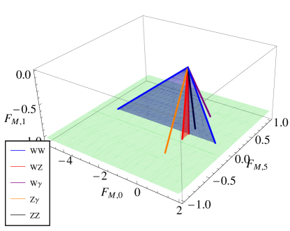
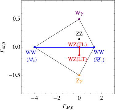
Figure 6: Left: the vectors $\vec{x}_{i}(\vec{a},\vec{b})$ intersect the plane $(u,-1,v)$, leaving a set of intersection points. Right: the intersection points $\vec{P}_{i}(\vec{a},\vec{b})=(u,v)$ on the plane. The colors represent different scattering channels. The $M_{\parallel}$, $\bar{M}_{\parallel}$, $LT$ and $TL$ in the brackets denote the corresponding polarisation configuration that gives the endpoints of the line segments, see Table 1 in Section 3.3.

Note that the $\vec{x}_{WW}$ and $\vec{x}_{WZ}$ are functions of $\vec{a},\vec{b}$ and they each span a triangle that intersects the plane with a line segment. Now we focus on the intersection points of $\vec{x}_{i}$, which we denote by $\vec{P}_{i}(\vec{a},\vec{b})=(u,v)$. They are

$$\vec{P}_{WW}(\vec{a},\vec{b})=\left(-\frac{4T_{a}T_{b}\cos\phi}{T_{a}^{2}-T_{a}T_{b}\cos\phi+T_{b}^{2}},0\right),\quad\vec{P}_{ZZ}(\vec{a},\vec{b})=\left(0,\frac{s_{W}^{2}}{2c_{W}^{2}}\right),$$ (60)

$$\vec{P}_{WZ}(\vec{a},\vec{b})=\left(0,-\frac{s_{W}^{2}T_{a}^{2}}{2c_{W}^{2}T_{a}^{2}+2T_{b}^{2}}\right),\quad\vec{P}_{W\gamma}(\vec{a},\vec{b})=\left(0,\frac{1}{2}\right),$$ (61)

$$\vec{P}_{Z\gamma}(\vec{a},\vec{b})=\left(0,-\frac{1}{2}\right).$$ (62)

These points are shown in Figure 6 right. From the above expressions we can see that, in this simplified case, depending on the polarisation, the $WW$ channel leads to intersection points on the horizontal axis, varying from -4 to 4/3, while the $WZ$ channel leads to intersection points on the vertical axis, varying from 0 to $-t_{W}^{2}/2$. In more general cases, the intersection points could form a higher dimensional point set, instead of just line segments.

Now we can use Eq. (58) to remove redundant conditions. When this equation is satisfied, the corresponding intersection point $\vec{P}$ of $\vec{x}$ must satisfy

$$\vec{P}=\sum_{i,j}c_{i,j}\vec{P}_{i}(\vec{a}_{j},\vec{b}_{j})$$ (63)

$$\sum_{i,j}c_{i,j}=1$$ (64)

i.e. the $\vec{P}$ is a positive linear combination of other intersection points, and that the sum of the coefficients is one. The latter condition comes from the fact that the second component of $\vec{x}$ is always -1. This implies that $\vec{P}$ stays within a polygon formed by other $\vec{P}_{i}(\vec{a}_{j},\vec{b}_{j})$. Therefore, in Figure 6 right, we are allowed to remove any points that are inside a polygon formed by other points. Obviously, the largest polygon is the convex hull of all $\vec{P}_{i}$, displayed by the black lines in the figure. It has four vertices, given respectively by the $W\gamma$ channel, the $WZ$ channel, and the $WW$ channel with two different polarisation states, which we denote as $M_{\parallel}$ and $\bar{M}_{\parallel}$. The polarisation will be better explained in Section 3.3. Here we simply mention that $M_{\parallel}$ means that $\vec{a}$ and $\vec{b}$ are parallel to each other, while $M_{\parallel}$ means that $\vec{a}$ and $\vec{b}^{\prime}$ are parallel to each other, where $\vec{b}^{\prime}=(b_{1},b_{2},-b_{3})$. With these four vertices, the positivity constraints are minimally described by four linear inequalities:

$$\begin{aligned} &-2F_{M,1}+F_{M,5}>0,\\ &-2F_{M,1}-F_{M,5}>0,\end{aligned}\quad\begin{aligned} &-4F_{M,0}-F_{M,1}>0,\\ &+4F_{M,0}-3F_{M,1}>0.\end{aligned}$$ (65)

These conditions solely are equivalent to the statement that Eq. (50) holds for any and all $\vec{a}$ and $\vec{b}$. We can rewrite the above solution in a form that is more convenient for a parameter scan,

$$F_{M,1}\in\left(-\infty,0\right)$$ (66)

$$F_{M,0}\in\left(\frac{3}{4}F_{M,1},-\frac{1}{4}F_{M,1}\right)$$ (67)

$$F_{M,5}\in\left(2F_{M,1},-2F_{M,1}\right)$$ (68)

It’s easy to see that these conditions carve out a pyramid in the 3-dimensional parameter space spanned by $F_{M,0}$, $F_{M,1}$ and $F_{M,5}$. We show this in Figure 7. Note that if we take $F_{M,5}=0$, the bounds in the $F_{M,0}-F_{M,1}$ plane are not as tight as we have shown in Figure 1 left. This is because here we only considered real polarisation vectors. If we allow $\vec{a}$ and $\vec{b}$ to take complex values, the $ZZ$ point will expand to a horizontal line that goes from $-\infty$ to $+2$, which leads to a stronger constraint.

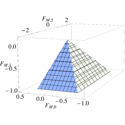
Figure 7: In a subspace spanned by three coefficients, $F_{M,0}$, $F_{M,1}$ and $F_{M,5}$, allowed parameter space is described by a pyramid.

In principle, the above procedure should apply to the most general case. However, the large dimension of the problem (18 coefficients) and the complex values of $\vec{a}$ and $\vec{b}$ components (6 degrees of freedom, after removing 4 free phases and 2 overall scaling factors), make the problem more complicated. We will solve the problem in two steps. In the first step, we focus on each channel, and remove the polarisation dependence in each channel. This corresponds to identifying the endpoints of the $WW$ and $WZ$ line segments in Figure 6 right. As we have mentioned, in a more general case, the $\vec{P}_{i}(\vec{a},\vec{b})$ points could form a higher dimensional object. In that case we will identify the boundary of this point set. In the second step, we combine the results of all channels, and simplify further. This is similar to removing the $ZZ$, $WZ(LT)$ and $WZ(TL)$ points in Figure 6 right by taking a convex hull of all points (here $(LT)$ and $(TL)$ denote two polarisation configurations which correspond to $W_{L}Z_{T}$ scattering and $W_{T}Z_{L}$ scattering respectively, see Table 1 in Section 3.3 for more details).

3.1.2 The cone case

There is still a caveat in the above approach: the boundary of the point set $\{\vec{P}_{i}(\vec{a},\vec{b})\}$ could be a curve. In that case taking the convex hull does not help to simplify its description. Consider a second example, where we turn on three different operators, $F_{S,0}$, $F_{M,0}$, and $F_{T,0}$. The corresponding $\vec{x}_{i}$ vectors are

$$\vec{x}_{WW}=\left(T_{a}^{2}T_{b}^{2},-T_{a}T_{b}\cos\phi,2\cos^{2}\phi\right)$$ (69)

$$\vec{x}_{ZZ}=\left(T_{a}^{2}T_{b}^{2},0,4c_{W}^{4}\cos^{2}\phi\right)$$ (70)

$$\vec{x}_{WZ}=(1,0,0)$$ (71)

$$\vec{x}_{Z\gamma}=\vec{x}_{\gamma\gamma}=(0,0,1)$$ (72)

$\vec{x}_{W\gamma}$ does not give any nontrivial result. We can see that the sum of the first and the third components are alway positive, i.e. these $\vec{x}$’s are always positive along the direction of $(1,0,1)$. Therefore similar to the previous case, we consider the intersection points of $\vec{x}_{i}$ on the plane

$$\vec{x}=\left(\frac{1+v}{\sqrt{2}},u,\frac{1-v}{\sqrt{2}}\right)$$ (73)

This is shown in Figure 8 left. In particular, we see that the $WW$ channel spans a cone that intersects the plain with a circle. Again, denoting the intersection points by $\vec{P}_{i}(\vec{a},\vec{b})=(u,v)$, we find

$$\vec{P}_{WW}(\vec{a},\vec{b})=\left(-\frac{\sqrt{2}T_{a}T_{b}\cos\phi}{T_{a}^{2}T_{b}^{2}+2\cos^{2}\phi},\frac{T_{a}^{2}T_{b}^{2}-2\cos^{2}\phi}{T_{a}^{2}T_{b}^{2}+2\cos^{2}\phi}\right),\qquad\vec{P}_{ZZ}(\vec{a},\vec{b})=\left(0,\frac{T_{a}^{2}T_{b}^{2}-4c_{W}^{4}\cos^{2}\phi}{T_{a}^{2}T_{b}^{2}+4c_{W}^{4}\cos^{2}\phi}\right),$$ (74)

$$\vec{P}_{WZ}(\vec{a},\vec{b})=(0,1),\qquad\vec{P}_{Z\gamma}(\vec{a},\vec{b})=P_{\gamma\gamma}(\vec{a},\vec{b})=(0,-1).$$ (75)

The intersection points are shown in Figure 8 right. We see that the $WW$ channel leaves a circle on the plane: if we define $\cot\frac{\theta}{2}=-\frac{T_{a}T_{b}}{\sqrt{2}\cos\phi}$, then

$$P_{WW}(\theta)=\left(\frac{1}{2}\sin\theta,\cos\theta\right)$$ (76)

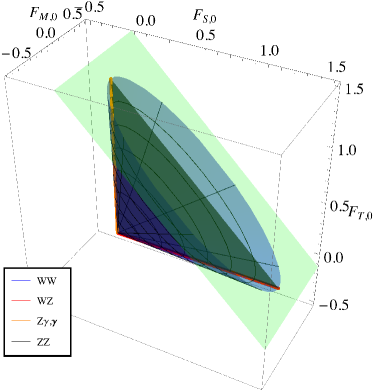
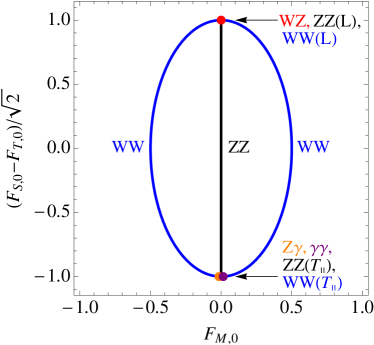
Figure 8: Similar to Figure 6. Left: the vectors $\vec{x}_{i}(\vec{a},\vec{b})$ intersect the plane $\left(\frac{1+v}{\sqrt{2}},u,\frac{1-v}{\sqrt{2}}\right)$, leaving a set of intersection points. Right: the intersection points $\vec{P}_{i}(\vec{a},\vec{b})=(u,v)$ on the plane form a circle. Colors represent different scattering channels. The $T_{\parallel}$ and $L$ in the brackets denote the corresponding polarisation configuration in the $WW$ and $ZZ$ channels that give the top and bottom points, see Table 1 in Section 3.3.

In this case, taking a convex hull allows us to keep only the $WW$ channel while removing all other channels, but the positivity is still described by an infinite set of vectors. To solve the exact condition, we note that $f_{WW}=\vec{F}\cdot\vec{x}_{WW}(\vec{a},\vec{b})$ is a quadratic function of $T_{a}T_{b}/\cos\phi$:

$$f_{WW}\propto F_{S,0}(T_{a}T_{b}/\cos\phi)^{2}-F_{M,0}(T_{a}T_{b}/\cos\phi)+2F_{T,0}$$ (77)

defined on $T_{a}T_{b}/\cos\phi\in(-\infty,\infty)$. The condition for this function to be positive is simply

$$F_{S,0}>0\qquad\mbox{and}\qquad 8F_{S,0}F_{T,0}-F_{M,0}^{2}>0$$ (78)

So even though the original inequality is a linear function of $\vec{F}$, by removing the $\vec{a}$ and $\vec{b}$ dependence the solution is upgraded to a quadratic function. This is because the most constraining value of $T_{a}T_{b}/\cos\phi$ is a function of the $F_{i}$ coefficients, which in this case is

$$\frac{T_{a}T_{b}}{\cos\phi}\to\frac{F_{M,0}}{2F_{S,0}}$$ (79)

and so $f_{WW}=\vec{F}\cdot\vec{x}_{WW}(T_{a}T_{b})$ becomes a quadratic function once the above value is plugged in. This quadratic function describes a cone in the parameter space spanned by $F_{S,0}$, $F_{M,0}$ and $F_{T,0}$. If we rotate the $S$ and $T$ axes by defining:

$$F_{1}=\frac{F_{S,0}+F_{T,0}}{\sqrt{2}}$$ (80)

$$F_{2}=\frac{F_{S,0}-F_{T,0}}{\sqrt{2}}$$ (81)

Then the condition can be written as

$$F_{1}^{2}>F_{2}^{2}+(F_{M,0}/2)^{2}$$ (82)

This carves out a cone with its vertex right at the origin and the axis pointing to the $F_{1}$ direction. We show this in Figure 9. Note that if we allow complex polarisation, the line segment from $ZZ$ channel will expand to an even larger circle, reducing the allowed parameter space to $4F_{S,0}F_{T,0}-F_{M,0}^{2}>0$.

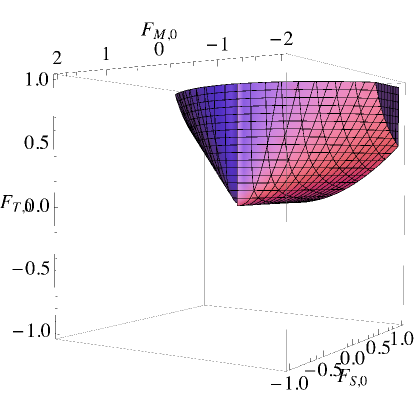
Figure 9: In a subspace spanned by three coefficients, $F_{S,0}$, $F_{M,0}$ and $F_{T,0}$, allowed parameter space is described by a cone.

In more general cases, i.e. with more operator coefficients and complex polarisation, solving the positivity condition of each channel will lead to several inequalities independent of polarisation. Some of them are linear inequalities. They are like the endpoints of the $WW$ and $WZ$ line segments in our first toy example. Others are quadratic or even higher order inequalities. They are like the cones as in our second example.

3.2 General solution

Now we consider the most general case.

First of all, it is useful to rewrite $x_{i}$ in a different form to remove the redundant degrees of freedom in $\vec{a}$ and $\vec{b}$. Since they are complex vectors, in total they have 12 degrees of freedom. However, the rescaling of $\vec{a}$ and $\vec{b}$ does not change the positivity condition. This removes 2 degrees of freedom. In addition, since the bounds are derived from the forward scattering amplitude, the system has a rotational symmetry around the beam axis, so the transversal components of the two vectors can appear only in the forms of $a_{1}b_{1}^{*}+a_{2}b_{2}^{*}$, $a_{1}b_{1}+a_{2}b_{2}$, $|a_{1}|^{2}+|a_{2}|^{2}$ and $|b_{1}|^{2}+|b_{2}|^{2}$. This removes 2 more degrees of freedom. Finally, $\vec{a}$, $\vec{b}$, $\vec{a}^{*}$ and $\vec{b}^{*}$ each appear once in the amplitude, so adding a pure phase on all components of either $\vec{a}$ or $\vec{b}$ does not change the result. This leads to two more redundant degrees of freedom. As a result, if we define:

$$|a_{3}|^{2}=T_{a}^{2},\quad|b_{3}|^{2}=T_{b}^{2}$$

$$a_{3}b_{3}^{*}=T_{a}T_{b}e^{i\delta},\quad a_{3}b_{3}=T_{a}T_{b}e^{i\Delta}$$

$$a_{1}b_{1}^{*}+a_{2}b_{2}^{*}=\cos\phi e^{i(\alpha+\delta)},\quad a_{1}b_{1}+a_{2}b_{2}=\cos\psi e^{i(\beta+\Delta)}$$

$$|a_{1}|^{2}+|a_{2}|^{2}=1,\quad|b_{1}|^{2}+|b_{2}|^{2}=1$$ (83)

then $x_{i}(\vec{a},\vec{b})$ only depend on six parameters: $T_{a}$, $T_{b}$, $\cos\phi$, $\cos\psi$, $\cos\alpha$ and $\cos\beta$. We have rescaled the both vectors to fix $|a_{1}|^{2}+|a_{2}|^{2}$ and $|b_{1}|^{2}+|b_{2}|^{2}$. $\delta$ and $\Delta$ are the free phases. The six parameters can take real values in the region

$$T_{a},T_{b}\in[0,+\infty)$$

$$\cos\phi,\cos\psi\in[0,1]$$

$$\cos\alpha,\cos\beta\in[-1,1]$$ (84)

It is easy to show that these 6 parameters can independently take any values in the above range, i.e. the change of variable can be inverted in the region defined above. Also, at this point one can see that the $W^{\pm}W^{\pm}$ and the $W^{\pm}W^{\mp}$ channels give the same bounds, because

$$\vec{x}_{W^{\pm}W^{\mp}}\left(T_{a},T_{b},\phi,\psi,\alpha,\beta\right)=\vec{x}_{W^{\pm}W^{\pm}}\left(T_{a},T_{b},\phi,\psi,\pi-\beta,\alpha\right)$$ (85)

So we will only consider $W^{\pm}W^{\pm}$, which we simply refer to as $WW$.

The problem now is the following: under which conditions are $\sum_{i}F_{i}x_{i}(\vec{a},\vec{b})$, as functions of the variables defined in Eq. (83), positive definite in the region defined by Eq. (84)? We will show that these functions, after additional changes of variables, are either at most quadratic functions defined in this area, or bounded by such functions from below. The positivity condition is then equivalent to two conditions, 1) the minimum values for these quadratic functions exist, and 2) the minimum values are positive. These two conditions can be decomposed into a set of linear inequalities, which are like the endpoints of $WW$ and $WZ$ line segments in our first toy example, plus one or two higher-degree polynomial inequalities, which are like the circle from $WW$ channel in our second example. Below we consider each channel separately.

3.2.1 $WW$

Let us first consider $WW$ scattering. For later convenience, we rewrite $\cos\phi$ as $W$, $\cos\psi$ as $V$, and $\cos\alpha$ as $R$. The positivity condition implies $f_{WW}\geq 0$, where $f_{WW}$ can be written as

$$f_{WW}(T_{a},T_{b},R,W,V)=f_{1}(T_{a}^{2}+T_{b}^{2})+f_{2}T_{a}^{2}T_{b}^{2}+f_{3}W^{2}+f_{4}T_{a}T_{b}RW+f_{5}V^{2}+f_{6}$$ (86)

where $T_{a}$, $T_{b}$, $W$, $R$, $V$ are independent parameters in the range

$$T_{a},T_{b}\in[0,+\infty),\quad W\in[0,1],\quad R\in[-1,1],\quad V\in[0,1]$$ (87)

and

$$f_{1}=-2F_{M,1}+F_{M,7}$$ (88)

$$f_{2}=8F_{S,0}+4F_{S,1}+4F_{S,2}$$ (89)

$$f_{3}=16F_{T,0}+8F_{T,1}+2F_{T,2}$$ (90)

$$f_{4}=-8F_{M,0}+2F_{M,1}-2F_{M,7}$$ (91)

$$f_{5}=16F_{T,1}+2F_{T,2}$$ (92)

$$f_{6}=6F_{T,2}$$ (93)

For $f_{WW}>0$ to hold for any $T_{a,b}$, $W$, $V$, $R$, two conditions need to be satisfied: 1) the minimal value of $f_{WW}$ exists, and 2) the minimal value is positive.

Because $f_{WW}(T_{a},T_{b},R,W,V)$ is a polynomial, the first condition only requires that its asymptotic values for large $T_{a,b}$ are positive. This implies

$$f_{1}>0,\ f_{2}>0$$ (94)

For the second condition we need to find its minimal value. Using $T_{a}^{2}+T_{b}^{2}\geq 2T_{a}T_{b}$ and $WT_{a}T_{b}\geq 0$, and defining $Z=T_{a}T_{b}>0$, we have

$$f_{WW}(T_{a},T_{b},R,W,V)\geq f^{\prime}_{WW}(Z,W,V)\equiv f_{2}Z^{2}+(2f_{1}-W|f_{4}|)Z+f_{3}W^{2}+f_{5}V^{2}+f_{6}$$ (95)

Minimizing $f^{\prime}_{WW}$ as a function of $Z$ implies

$$Z\to-\frac{2f_{1}-W|f_{4}|}{2f_{2}}$$ (96)

However $Z$ must be positive, so the at this step the minimal value of $f^{\prime}_{WW}$ is

$$\min f^{\prime}_{WW}(Z)=\left\{\begin{array}[]{ll}W|f_{4}|>2f_{1}:&W^{2}f_{3}+f_{5}V^{2}+f_{6}-\frac{(2f_{1}-W|f_{4}|)^{2}}{4f_{2}}\\ W|f_{4}|<=2f_{1}:&W^{2}f_{3}+f_{5}V^{2}+f_{6}\end{array}\right.$$ (99)

Now we need to minimize this function w.r.t $W$. If $|f_{4}|<=2f_{1}$, then $W|f_{4}|<=2f_{1}$ always holds. In this case we have

$$\min f^{\prime}_{ZZ}(Z,W)=\min W^{2}f_{3}+f_{5}V^{2}+f_{6}$$

$$= \left\{\begin{array}[]{ll}f_{3}\geq 0:&f_{5}V^{2}+f_{6}\\ f_{3}<0:&f_{3}+f_{5}V^{2}+f_{6}\end{array}\right.$$ (102)

On the other hand, if $|f_{4}|>2f_{1}$, we define $W_{c}=2f_{1}/|f_{4}|$. In this case $\min f^{\prime}_{WW}(Z)$ as a function of $W$ is a piecewise function defined on $W\in[0,1]$:

$$\min f^{\prime}_{WW}(Z)=\left\{\begin{array}[]{ll}0<=W<=W_{c}:&W^{2}f_{3}+f_{5}V^{2}+f_{6}\\ W_{c}<W<=1:&W^{2}f_{3}+f_{5}V^{2}+f_{6}-\frac{(2f_{1}-W|f_{4}|)^{2}}{4f_{2}}\end{array}\right.$$ (105)

Now

• if $f_{3}\geq\frac{f_{4}^{2}}{4f_{2}}$, the above function is a monotonically increasing function of $W$ in $[0,1]$, so we take $W\to 0$ and $\min f^{\prime}_{WW}(Z,W)=f_{5}$.

• If $\frac{(2f_{1}-|f_{4}|)^{2}}{4f_{2}}<=f_{3}<\frac{f_{4}^{2}}{4f_{2}}$, the above function is a monotonically increasing function of $W$ in $[0,W_{c}]$ and is a concave function of $W$ in $(W_{c},1]$. By comparing its value at $W=0$ and $W=1$, i.e. $f_{5}V^{2}+f_{6}$ and $f_{5}V^{2}+f_{6}+f_{3}-\frac{(2f_{1}-|f_{4}|)^{2}}{4f_{2}}$, we find $\min f^{\prime}_{WW}(Z,W)=f_{5}V^{2}+f_{6}$.

• Similarly, if $0<=f_{3}<\frac{(2f_{1}-|f_{4}|)^{2}}{4f_{2}}$, we find $\min f^{\prime}_{WW}(Z,W)=f_{5}V^{2}+f_{6}+f_{3}-\frac{(2f_{1}-|f_{4}|)^{2}}{4f_{2}}$.

• Finally, if $f_{3}<0$, the function is monotonically decreasing in $[0,1]$, so $\min f^{\prime}_{WW}(Z,W)=f_{5}V^{2}+f_{6}+f_{3}-\frac{(2f_{1}-|f_{4}|)^{2}}{4f_{2}}$.

Finally, the function is linear in $V^{2}$. Putting pieces together, we obtain

$$\min f^{\prime}_{WW}(W,V,Z) =f_{6}+\min\left(f_{5},0\right)+\min\left(0,f_{3}-\frac{\max(0,-2f_{1}+|f_{4}|)^{2}}{4f_{2}}\right)$$ (106)

and this needs to be positive. Together with Eq. (94), $f_{WW}>0$ is equivalent to the combination of the following linear conditions:

$$f_{1}>0,f_{2}>0,f_{6}>0,f_{3}+f_{6}>0,f_{5}+f_{6}>0,f_{3}+f_{5}+f_{6}>0$$ (107)

and the following quadratic inequalities:

$$4f_{2}(f_{3}+f_{6})>\max(0,|f_{4}|-2f_{1})^{2},$$ (108)

$$4f_{2}(f_{3}+f_{5}+f_{6})>\max(0,|f_{4}|-2f_{1})^{2},$$ (109)

3.2.2 $ZZ$

For $ZZ$ and all the other scattering channels, we use a different change of variables

$$\cos^{2}\phi+\cos^{2}\psi=2W^{2}$$ (110)

$$\cos\phi\cos\alpha-\cos\psi\cos\beta=2WR$$ (111)

and again, $T_{a}$, $T_{b}$, $W$, $R$ are independent parameters in the range

$$T_{a},T_{b}\in[0,+\infty),\quad W\in[0,1],\quad R\in[-1,1]$$ (112)

The positivity condition from $ZZ$ channel requires $f_{ZZ}>0$, where

$$f_{ZZ}(T_{a},T_{b},R,W)=g_{1}(T_{a}^{2}+T_{b}^{2})+g_{2}T_{a}^{2}T_{b}^{2}+g_{3}W^{2}+g_{4}T_{a}T_{b}RW+g_{5}$$ (113)

and

$$g_{1}=-2c_{W}^{6}F_{M,1}+c_{W}^{6}F_{M,7}+c_{W}^{4}s_{W}^{2}F_{M,5}-c_{W}^{2}s_{W}^{4}F_{M,3}$$ (114)

$$g_{2}=8c_{W}^{4}F_{S,0}+8c_{W}^{4}F_{S,1}+8c_{W}^{4}F_{S,2}$$ (115)

$$g_{3}=32c_{W}^{8}F_{T,0}+32c_{W}^{8}F_{T,1}+16c_{W}^{4}s_{W}^{4}F_{T,5}+16c_{W}^{4}s_{W}^{4}F_{T,6}+4c_{W}^{4}s_{W}^{4}F_{T,7}$$

$$+8{c_{W}^{8}}F_{T,2}+8s_{W}^{8}F_{T,8}+2s_{W}^{8}F_{T,9}$$ (116)

$$g_{4}=-16c_{W}^{6}F_{M,0}+4c_{W}^{6}F_{M,1}-2c_{W}^{6}F_{M,7}-8c_{W}^{4}s_{W}^{2}F_{M,4}-2c_{W}^{4}s_{W}^{2}F_{M,5}$$

$$-8c_{W}^{2}s_{W}^{4}F_{M,2}+2c_{W}^{2}s_{W}^{4}F_{M,3}$$ (117)

$$g_{5}=8c_{W}^{8}F_{T,2}+4c_{W}^{4}s_{W}^{4}F_{T,7}+2s_{W}^{8}F_{T,9}$$ (118)

Now $f_{ZZ}$ has exactly the same form as $f_{WW}(T_{a},T_{b},R,W,0)$, as defined in Eq. (95). Therefore we can directly obtain the similar results:

$$g_{1}>0,g_{2}>0,g_{5}>0,g_{3}+g_{5}>0,$$ (119)

and one additional quadratic inequality:

$$4g_{2}(g_{3}+g_{5})>\max(0,|g_{4}|-2g_{1})^{2}.$$ (120)

3.2.3 $WZ$

The positivity condition from the $WZ$ channel requires $f_{WZ}>0$, where

$$f_{WZ}(T_{a},T_{b},R,W)=h^{\prime}_{1}T_{a}^{2}+h^{\prime\prime}_{1}T_{b}^{2}+h_{2}T_{a}^{2}T_{b}^{2}+h_{3}W^{2}+h_{4}T_{a}T_{b}RW+h_{5}$$ (121)

where

$$h^{\prime}_{1}=-2c_{W}^{4}F_{M,1}+c_{W}^{4}F_{M,7}-c_{W}^{2}s_{W}^{2}F_{M,5}-s_{W}^{4}F_{M,3}$$ (122)

$$h^{\prime\prime}_{1}=c_{W}^{2}F_{M,7}-2c_{W}^{2}F_{M,1}$$ (123)

$$h_{2}=4c_{W}^{2}F_{S,0}+4c_{W}^{2}F_{S,2}$$ (124)

$$h_{3}=16c_{W}^{4}F_{T,1}+4s_{W}^{4}F_{T,6}$$ (125)

$$h_{4}=-2c_{W}^{3}F_{M,7}-4c_{W}s_{W}^{2}F_{M,4}-c_{W}s_{W}^{2}F_{M,5}$$ (126)

$$h_{5}=4c_{W}^{4}F_{T,2}+s_{W}^{4}F_{T,7}$$ (127)

This is similar to the previous cases, and the only difference is that $T_{a}^{2}$ and $T_{b}^{2}$ have different coefficients. The minimal value exists if and only if

$$h^{\prime}_{1}>0,\ h^{\prime\prime}_{1}>0,\ h_{2}>0$$ (128)

Similar to the $WW$ and $ZZ$ cases, using $h^{\prime}_{1}T_{a}^{2}+h^{\prime\prime}_{1}T_{b}^{2}\geq 2\sqrt{h^{\prime}_{1}h^{\prime\prime}_{1}}T_{a}T_{b}$, $T_{a}T_{b}W\geq 0$, and defining $Z\equiv T_{a}T_{b}$, $h_{1}\equiv\sqrt{h^{\prime}_{1}h^{\prime\prime}_{1}}$, we have

$$f_{WZ}(T_{a},T_{b},R,W)\geq f^{\prime}_{WZ}(Z,W)=h_{2}Z^{2}+\left(2h_{1}-W|h_{4}|\right)Z+h_{3}W^{2}+h_{5}$$ (129)

This function has exactly the same form as $f^{\prime}_{WW}(Z,W,V=0)$, so we can use directly use the result there to obtain

$$h^{\prime}_{1}>0,h^{\prime\prime}_{1}>0,h_{2}>0,h_{5}>0,h_{3}+h_{5}>0$$ (130)

and one addition inequality:

$$4h_{2}(h_{3}+h_{5})>\max\left(0,|h_{4}|-2\sqrt{h^{\prime}_{1}h^{\prime\prime}_{1}}\right)^{2},$$ (131)

Because of the square root on the r.h.s., this is a quartic inequality.

3.2.4 $W\gamma$, $Z\gamma$ and $\gamma\gamma$

The positivity conditions require $f_{W\gamma,Z\gamma,\gamma\gamma}\geq 0$, where

$$f_{W\gamma}(T_{a},T_{b},R,W)=i_{1}T_{a}^{2}+i_{2}W^{2}+i_{3}$$ (132)

$$f_{Z\gamma}(T_{a},T_{b},R,W)=j_{1}T_{a}^{2}+j_{2}W^{2}+j_{3}$$ (133)

$$f_{\gamma\gamma}(T_{a},T_{b},R,W)=k_{2}W^{2}+k_{3}$$ (134)

where

$$i_{1}=-2F_{M,1}-F_{M,3}+F_{M,5}+F_{M,7}$$ (135)

$$i_{2}=16F_{T,1}+4F_{T,6}$$ (136)

$$i_{3}=4F_{T,2}+F_{T,7}$$ (137)

$$j_{1}=-2c_{W}^{2}F_{M,1}-c_{W}^{2}F_{M,3}-c_{W}^{2}F_{M,5}+c_{W}^{2}F_{M,7}$$ (138)

$$j_{2}=32c_{W}^{4}F_{T,0}+32c_{W}^{4}F_{T,1}+8s_{W}^{4}F_{T,8}+2s_{W}^{4}F_{T,9}+8c_{W}^{4}F_{T,2}-16s_{W}^{2}c_{W}^{2}F_{T,5}$$

$$+4\left(c_{W}^{2}-s_{W}^{2}\right)^{2}F_{T,6}-4s_{W}^{2}c_{W}^{2}F_{T,7}$$ (139)

$$j_{3}=8c_{W}^{4}F_{T,2}+2s_{W}^{4}F_{T,9}+\left(c_{W}^{2}-s_{W}^{2}\right)^{2}F_{T,7}$$ (140)

$$k_{2}=16F_{T,0}+16F_{T,1}+4F_{T,2}+8F_{T,5}+8F_{T,6}+2F_{T,7}+4F_{T,8}+F_{T,9}$$ (141)

$$k_{3}=4F_{T,2}+2F_{T,7}+F_{T,9}$$ (142)

These functions have similar forms. They are linear functions of $T_{a}^{2}\in[0,+\infty)$ and $W^{2}\in[0,1]$, so they are positive if and only if

$$i_{1}>0,\ j_{1}>0,$$ (143)

$$i_{3}>0,\ j_{3}>0,\ k_{3}>0,$$ (144)

$$i_{2}+i_{3}>0,\ j_{2}+j_{3}>0,\ k_{2}+k_{3}>0$$ (145)

i.e. these three channels only give rise to linear constraints in the parameter space.

3.3 Polarisation

Our final result is the combination of constraints described by Eqs. (107), (108), (109), (119), (120), (130), (131), (143), (144) and (145). However, it remains to show that these bounds can be actually achieved. This can be demonstrated by showing that the changes of variables we have used in Eq. (83) can be inverted, and therefore the minimum value of $f$ can always be reached by some physical polarisation state.

Here instead, we will directly give the explicit polarisation vectors $\vec{a}$ and $\vec{b}$ that will lead to all the resulting bounds. These are physically the most crucial values for $\vec{a}$ and $\vec{b}$: once positivity bounds for them are satisfied, then the same bounds are also satisfied for arbitrary polarisation. With them it is also more convenient to check that all these conditions can be reached, as one can simply plug in the corresponding $\vec{a}$ and $\vec{b}$ values into the original positivity conditions in Eqs. (36)-(43), and obtain our main results in Eqs. (107), (108), (109), (119), (120), (130), (131), (143), (144) and (145) right away. These polarisation values are obtained by keeping track of the values of $\vec{a}$ and $\vec{b}$ when we look for the minimal values and asymptotic values of $f_{VV^{\prime}}$. In a sense they correspond the boundary of the polarisation space once mapped to the space of $x_{i}$.

For convenience, in Table 1 we define notations for the polarisation cases that are relevant and useful for later presentation. For example, $L$ and $T$ represent the cases of two longitudinal vectors and two transversal vectors, and as we will see they naturally lead to bounds on the $S$-type and $T$-type operators. The $T$ case can further be divided into four cases which lead to different constraints. They represent two vectors with parallel polarisation, perpendicular polarisation, and those with $++$ (or $--$) and $+-$ helicity states. $TL$ and $LT$ denote the scattering between one transversal vector and one longitudinal vector, and are expected to constrain the $M$-type operators. The $M$ and $\bar{M}$ polarisation are mixtures of transversal and longitudinal states, which could give quadratic or quartic bounds. The subscripts in this case only represent the relation of the transversal components $(a_{1},a_{2})$ and $(b_{1},b_{2})$. In particular the $M_{I}({\bar{M}}_{I})$ is a special case of $M_{\parallel}({\bar{M}}_{\parallel})$, where a relative phase of $\pi/2$ between the longitudinal and the transversal parts is required. Finally, the $M^{\prime}$ and $\bar{M}^{\prime}$ case requires a special relation between $a_{3}/\sqrt{a_{1}^{2}+a_{2}^{2}}$ and $b_{3}/\sqrt{b_{1}^{2}+b_{2}^{2}}$. This applies to the $WZ$ channel only.

$$\begin{array}[]{|l|l|l|l|}\hline\cr&\text{Notation}&\text{Example of $a_{i},b_{i}$ values}&\text{General form}\\ \hline\cr\hline\cr\hbox{\multirowsetup Linear}&L&\vec{a}=(0,0,1),\vec{b}=(0,0,1)&\vec{a}=(0,0,m),\vec{b}=(0,0,n)\\ \cline{2-4}\cr&LT&\vec{a}=(0,0,1),\vec{b}=(1,0,0)&\vec{a}=(0,0,m_{3}),\vec{b}=(n_{1},n_{2},0)\\ &TL&\vec{a}=(1,0,0),\vec{b}=(0,0,1)&\vec{a}=(m_{1},m_{2},0),\vec{b}=(0,0,n_{3})\\ \cline{2-4}\cr&T_{\perp}&\vec{a}=(1,0,0),\vec{b}=(0,1,0)&\vec{a}=e^{i\rho}(k_{1},k_{2},0),\vec{b}=e^{i\sigma}(k_{2},-k_{1},0)\\ &T_{\parallel}&\vec{a}=(1,0,0),\vec{b}=(1,0,0)&\vec{a}=e^{i\rho}(k_{1},k_{2},0),\vec{b}=e^{i\sigma}(k_{1},k_{2},0)\\ &T_{++}&\vec{a}=(1,i,0),\vec{b}=(1,-i,0)&\vec{a}=e^{i\rho}(k_{1},\pm ik_{1},0),\vec{b}=e^{i\sigma}(k_{1},\mp ik_{1},0)\\ &T_{+-}&\vec{a}=(1,i,0),\vec{b}=(1,i,0)&\vec{a}=e^{i\rho}(k_{1},\pm ik_{1},0),\vec{b}=e^{i\sigma}(k_{1},\pm ik_{1},0)\\ \hline\cr\hline\cr&M_{+-}&\vec{a}=(x,ix,1),\vec{b}=(x,ix,1)&\vec{a}=e^{i\rho}(k_{1},\pm ik_{1},e^{i\gamma}k_{3}),\vec{b}=e^{i\sigma}(k_{1},\pm ik_{1},e^{i\gamma}k_{3})\\ &M_{\parallel}&\vec{a}=(x,0,1),\vec{b}=(x,0,1)&\vec{a}=e^{i\rho}(k_{1},k_{2},e^{i\gamma}k_{3}),\vec{b}=e^{i\sigma}(k_{1},k_{2},e^{i\gamma}k_{3})\\ &M_{I}&\vec{a}=(ix,0,1),\vec{b}=(ix,0,1)&\vec{a}=e^{i\rho}(ik_{1},ik_{2},k_{3}),\vec{b}=e^{i\sigma}(ik_{1},ik_{2},k_{3})\\ \cline{2-4}\cr\mbox{Quadratic}&\bar{M}_{+-}&\vec{a}=(x,ix,1),\vec{b}=(x,ix,-1)&\vec{a}=e^{i\rho}(k_{1},\pm ik_{1},e^{i\gamma}k_{3}),\vec{b}=e^{i\sigma}(k_{1},\pm ik_{1},-e^{i\gamma}k_{3})\\ \mbox{and}&\bar{M}_{\parallel}&\vec{a}=(x,0,1),\vec{b}=(x,0,-1)&\vec{a}=e^{i\rho}(k_{1},k_{2},e^{i\gamma}k_{3}),\vec{b}=e^{i\sigma}(k_{1},k_{2},-e^{i\gamma}k_{3})\\ \mbox{quartic}&\bar{M}_{I}&\vec{a}=(ix,0,1),\vec{b}=(ix,0,-1)&\vec{a}=e^{i\rho}(ik_{1},ik_{2},k_{3}),\vec{b}=e^{i\sigma}(ik_{1},ik_{2},-k_{3})\\ \cline{2-4}\cr&M_{I}^{\prime}&\vec{a}=(ix,0,\sqrt{h_{1}^{\prime\prime}}),&\vec{a}=e^{i\rho}(ik_{1},ik_{2},k_{3}),\vec{b}=e^{i\sigma}(ik_{1},ik_{2},k^{\prime}_{3}),\\ &&\vec{b}=(ix,0,\sqrt{h_{1}^{\prime}})&h_{1}^{\prime}k_{3}^{2}=h_{1}^{\prime\prime}{k^{\prime}}_{3}^{2},k_{3}k^{\prime}_{3}>0\\ &\bar{M}^{\prime}_{I}&\vec{a}=(ix,0,\sqrt{h_{1}^{\prime\prime}}),&\vec{a}=e^{i\rho}(ik_{1},ik_{2},k_{3}),\vec{b}=e^{i\sigma}(ik_{1},ik_{2},k^{\prime}_{3}),\\ &&\vec{b}=(ix,0,-\sqrt{h_{1}^{\prime}})&h_{1}^{\prime}k_{3}^{2}=h_{1}^{\prime\prime}{k^{\prime}}_{3}^{2},k_{3}k^{\prime}_{3}<0\\ \hline\cr\hline\cr\vrule\lx@intercol\hfil m_{i},n_{i}\in\mathbb{C},\ x,k_{i},k^{\prime}_{i}\in\mathbb{R},\ \rho,\sigma,\gamma\in[0,2\pi)\hfil\lx@intercol\vrule\lx@intercol\\ \hline\cr\end{array}$$ (165)

Table 1: Notation for relevant polarisation configurations. The $L$, $LT$, $TL$ and $T_{i}$ cases lead to linear inequalities, while the $M_{i}$ and $\bar{M}_{i}$ cases lead to higher order inequalities. We show example values of $a_{i}$ and $b_{i}$, and in addition also give their general form in the last column.

We are now ready to collect all the solutions in the previous subsection, keeping track of the polarisation configurations that allow the conditions to be reached. First, collecting Eqs. (107), (108), (109), (119), (120), (130), (131), (143), (144) and (145), we find that the linear conditions can be decomposed into three subspaces, spanned respectively by the three classes of operator coefficients: the $F_{S,i}$ coefficients, the $F_{M,i}$ coefficients, and the $F_{T,i}$ coefficients, i.e.

$$M_{S,ij}F_{S,j}>0$$ (166)

$$M_{M,ij}F_{M,j}>0$$ (167)

$$M_{T,ij}F_{T,j}>0$$ (168)

where “>0” means that each component is positive, and

$$F_{S,i}=(F_{S,0},F_{S,1},F_{S,2})^{T}$$ (169)

$$F_{M,i}=(F_{M,0},F_{M,1},F_{M,2},F_{M,3},F_{M,4},F_{M,5},F_{M,7})^{T}$$ (170)

$$F_{T,i}=(F_{T,0},F_{T,1},F_{T,2},F_{T,5},F_{T,6},F_{T,7},F_{T,8},F_{T,9})^{T}$$ (171)

and the $M$ matrices are given by

$$M_{S}=\left(\begin{array}[]{ccc}2&1&1\\ 1&1&1\\ 1&0&1\\ \end{array}\right)\begin{array}[]{l}WW,L\\ ZZ,L\\ WZ,L\\ \end{array}$$ (178)

$$M_{M}=\left(\begin{array}[]{cccccccc}0&-2c_{W}^{4}&0&-s_{W}^{4}&0&s_{W}^{2}c_{W}^{2}&c_{W}^{4}\\ 0&-2c_{W}^{4}&0&-s_{W}^{4}&0&-s_{W}^{2}c_{W}^{2}&c_{W}^{4}\\ 0&-2&0&0&0&0&1\\ 0&-2&0&-1&0&1&1\\ 0&-2&0&-1&0&-1&1\\ \end{array}\right)\begin{array}[]{l}ZZ,LT\&TL\\ WZ,LT\\ WW,LT\&TL;WZ,TL\\ W\gamma,LT\\ Z\gamma,LT\\ \end{array}$$ (189)

$$M_{T}=\left(\begin{array}[]{ccccccccc}0&0&1&0&0&0&0&0\\ 0&2&1&0&0&0&0&0\\ 2&1&1&0&0&0&0&0\\ 8&12&5&0&0&0&0&0\\ 8c_{W}^{8}&8c_{W}^{8}&4c_{W}^{8}&4c_{W}^{4}s_{W}^{4}&4c_{W}^{4}s_{W}^{4}&2c_{W}^{4}s_{W}^{4}&2s_{W}^{8}&s_{W}^{8}\\ 0&0&4c_{W}^{8}&0&0&2c_{W}^{4}s_{W}^{4}&0&s_{W}^{8}\\ 0&0&4c_{W}^{4}&0&0&s_{W}^{4}&0&0\\ 0&16c_{W}^{4}&4c_{W}^{4}&0&4s_{W}^{4}&s_{W}^{4}&0&0\\ 0&0&4&0&0&1&0&0\\ 0&16&4&0&4&1&0&0\\ 0&0&8c_{W}^{4}&0&0&\left(c_{W}^{2}-s_{W}^{2}\right)^{2}&0&2s_{W}^{4}\\ 32c_{W}^{4}&32c_{W}^{4}&16c_{W}^{4}&-16c_{W}^{2}s_{W}^{2}&4\left(c_{W}^{2}-s_{W}^{2}\right)^{2}&1-8s_{W}^{2}c_{W}^{2}&8s_{W}^{4}&4s_{W}^{4}\\ 0&0&4&0&0&2&0&1\\ 8&8&4&4&4&2&2&1\\ \end{array}\right)\begin{array}[]{l}WW,T_{\perp}\\ WW,T_{++}\\ WW,T_{+-}\\ WW,T_{\parallel}\\ ZZ,T_{\parallel}\\ ZZ,T_{\perp}\\ WZ,T_{\perp}\\ WZ,T_{\parallel}\\ W\gamma,T_{\perp}\\ W\gamma,T_{\parallel}\\ Z\gamma,T_{\perp}\\ Z\gamma,T_{\parallel}\\ \gamma\gamma,T_{\perp}\\ \gamma\gamma,T_{\parallel}\\ \end{array}$$ (218)

For each row, we also give the channel and the corresponding polarisation state that leads to the very condition, to the right of the matrix. For example, the first row in $M_{S}$ simply means that the bound $2F_{S,0}+F_{S,1}+F_{S,2}>0$ can be obtained from the $WW$ scattering channel, by considering the $L$ polarisation, which is described by the first row in Table 1. One can easily check this by inserting the example values $\vec{a}=\vec{b}=(0,0,1)$ into the positivity condition Eq. (37). The same is true for other rows and other matrices.

Several comments are in order for these linear conditions:

• Each row in these matrices is a $\vec{x}(\vec{a},\vec{b})$ vector, with $\vec{a}$ and $\vec{b}$ taking the polarisation displayed to its right. Together they describe the “boundaries” of all $\vec{x}(\vec{a},\vec{b})$, just like the endpoints in our first toy exmaple in Section 3.1.

• The relevant polarisation states for linear conditions are either purely longitudinal, or purely transversal, or one vector boson is longitudinal and the other one transversal.

• The $T_{++}$ and $T_{+-}$ configurations require $\vec{a}$ and $\vec{b}$ to take complex values. This is one of the reasons why allowing for complex polarisation states will further restrict the parameter space. They give two additional constraints in the $T$ operator space. The other bounds are not affected.

• As discussed in our first toy example, each row of these matrices corresponds to some $\vec{x}_{i}$ vector, and once they are combined we may be able to simplify further by taking the convex hull of them. For $M_{S}$ and $M_{M}$, these vectors already form a convex pyramid, so taking a convex hull does not simplify the description. The $M_{T}$ however contains three vectors that stay inside some pyramids formed by other vectors. They are labeled by a $*$ before the corresponding channel, and so we can further remove these conditions. This will be further discussed in the next section.

• $F_{M,0}$, $F_{M,2}$, and $F_{M,4}$ are not subject to any linear constraints, but we will see that they are constrained by the higher order ones.

In addition, there are four higher order inequalities:

1. $WW$, $M_{+-}$ and $\bar{M}_{+-}$ polarisation

   $$4f_{2}(f_{3}+f_{6})>\max(0,|f_{4}|-2f_{1})^{2},$$ (219)

2. $WW$, $M_{\parallel}$ and $\bar{M}_{\parallel}$ polarizatoin

   $$4f_{2}(f_{3}+f_{5}+f_{6})>\max(0,|f_{4}|-2f_{1})^{2},$$ (220)

3. $ZZ$, $M_{I}$ and $\bar{M}_{I}$ polarisation

   $$4g_{2}(g_{3}+g_{5})>\max(0,|g_{4}|-2g_{1})^{2},$$ (221)

4. $WZ$, $M^{\prime}_{I}$ and $\bar{M}^{\prime}_{I}$ polarisation

   $$4h_{2}(h_{3}+h_{5})>\max\left(0,|h_{4}|-2\sqrt{h^{\prime}_{1}h^{\prime\prime}_{1}}\right)^{2},$$ (222)

Each condition has two relevant polarisation configurations, corresponding to the sign of the parameter in the absolute value function. For example, in the first condition, the $M_{+-}$ gives

$$4f_{2}(f_{3}+f_{6})>\max(0,-f_{4}-2f_{1})^{2},$$ (223)

while the $\bar{M}_{+-}$ gives

$$4f_{2}(f_{3}+f_{6})>\max(0,f_{4}-2f_{1})^{2},$$ (224)

The same is true for the other three conditions. In terms of the original coefficients, these four conditions are given below explicitly:

$$\framebox{$WW,\ M_{+-}\&\bar{M}_{+-}$}$$

$$32(2F_{S,0}+F_{S,1}+F_{S,2})(2F_{T,0}+F_{T,1}+F_{T,2})$$

$$-\max(0,4F_{M,0}+F_{M,1},-4F_{M,0}+3F_{M,1}-2F_{M,7})^{2}>0$$ (225)

$$\framebox{$WW,\ M_{\parallel}\&\bar{M}_{\parallel}$}$$

$$8(2F_{S,0}+F_{S,1}+F_{S,2})(8F_{T,0}+12F_{T,1}+5F_{T,2})$$

$$-\max(0,4F_{M,0}+F_{M,1},-4F_{M,0}+3F_{M,1}-2F_{M,7})^{2}>0$$ (226)

$$\framebox{$ZZ,\ M_{I}\&\bar{M}_{I}$}$$

$$8(F_{S,0}+F_{S,1}+F_{S,2})\left[4c_{W}^{8}(2F_{T,0}+2F_{T,1}+F_{T,2})+2c_{W}^{4}s_{W}^{4}(2F_{T,5}+2F_{T,6}+F_{T,7})\right.$$

$$\left.+s_{W}^{8}(2F_{T,8}+F_{T,9})\right]-\max\left[0,2\left(2c_{W}^{4}F_{M,0}+F_{M,2}s_{W}^{4}-F_{M,4}s_{W}^{4}+F_{M,4}s_{W}^{2}\right),\right.$$

$$\left.-c_{W}^{4}(4F_{M,0}-2F_{M,1}+F_{M,7})-2c_{W}^{2}F_{M,4}s_{W}^{2}-s_{W}^{4}(2F_{M,2}-F_{M,3})-F_{M,5}\left(s_{W}^{2}-s_{W}^{4}\right)\right]^{2}>0$$ (227)

$$\framebox{$WZ,\ M^{\prime}_{I}\&\bar{M}^{\prime}_{I}$}$$

$$16(F_{S,0}+F_{S,2})\left[4c_{W}^{4}(4F_{T,1}+F_{T,2})+s_{W}^{4}(4F_{T,6}+F_{T,7})\right]-\max\Big{[}0,+2c_{W}^{2}F_{M,7}$$

$$-2\sqrt{(2F_{M,1}-F_{M,7})\left(c_{W}^{4}(2F_{M,1}-F_{M,7})+c_{W}^{2}F_{M,5}s_{W}^{2}+F_{M,3}s_{W}^{4}\right)}+4F_{M,4}s_{W}^{2}+F_{M,5}s_{W}^{2},$$

$$-2c_{W}^{2}F_{M,7}-2\sqrt{(2F_{M,1}-F_{M,7})\left(c_{W}^{4}(2F_{M,1}-F_{M,7})+c_{W}^{2}F_{M,5}s_{W}^{2}+F_{M,3}s_{W}^{4}\right)}$$

$$-4F_{M,4}s_{W}^{2}-F_{M,5}s_{W}^{2}\Big{]}^{2}>0$$ (228)

where the 2nd and the 3rd terms in the $\max$ functions correspond to $M$ and $\bar{M}$ polarisations respectively.

Several comments are in order for these higher order inequalities:

• These inequalities come from the convex boundaries of all $\vec{x}(\vec{a},\vec{b})$, e.g. the circle in our second toy example in Section 3.1.

• While $WW$ and $ZZ$ give 3 quadratic inequalities, the $WZ$ channel involves square roots in the form given above, so the corresponding inequality is a quartic one.

• The polarisation states for quadratic conditions must involve both longitudinal and transversal components. Their ratio is only given as a free parameter $x$. By plugging in the example values given in Table 1, one will get a quadratic function of $x^{2}$. By requiring this function to be positive definite, the corresponding quadratic constraint will be obtained.

• The $M_{+-}$, $\bar{M}_{+-}$, $M_{I}$, $\bar{M}_{I}$, $M^{\prime}_{I}$ and $\bar{M}^{\prime}_{I}$ polarisation states require complex values of $\vec{a}$ and $\vec{b}$. If restricted to real values, we will only have the 2nd quadratic condition from $WW$. This is another reason why complex polarisation could further constrain the parameter space.

• The quadratic constraints from $WW$ and $ZZ$ have the following form:

  $$\left(\sum_{i}a_{i}F_{S,i}\right)\left(\sum_{i}b_{i}F_{T,i}\right)>\max\left(0,\sum_{i}c_{i}F_{M,i},\sum_{i}d_{i}F_{M,i}\right)^{2}$$ (229)

  i.e. a linear combination of $M$ coefficients being less than the geomatic mean of a linear combination of $S$ coefficients and another combination of $T$ coefficients. The two combinations on the l.h.s. have to be individually positive: this is included already in the linear conditions. Also, to see the full structure of this condition, one needs to turn on all three kinds of operators: $S$, $M$ and $T$.

• If one considers a subspace spanned by $F_{S,i}$ or $F_{T,i}$ operators only, the r.h.s. of Eq. (229) vanishes, while the two sums on the l.h.s. are already positive as required by the linear conditions. So the quadratic function becomes trivial in a subspace without $M$-type operators.

• On the other hand, if we consider a subspace spanned by $F_{M,i}$ operators, and setting other operators to zero, then the r.h.s. must also be zero. This implies that both

  $$\sum_{i}c_{i}F_{M,i}<0\quad\text{and}\quad\sum_{i}d_{i}F_{M,i}<0$$ (230)

  need to be satisfied. So in the $F_{M,i}$ space, the quadratic condition reduces to two linear conditions.

• Finally the quartic constraints from $WZ$ is also trivial in the $S$ and $T$ subspaces. In the $M$ subspace, however, the r.h.s. involves square roots. It implies that

  $$4h^{\prime}_{1}h^{\prime\prime}_{1}>h_{4}^{2}$$ (231)

  This is a quadratic condition that only involves $F_{M,i}$ operators. So unlike the $S$ and $T$ subspaces that are only constrained by linear bounds, the $M$ subspace is described by a set of linear bounds from $M_{M}$, another set of linear bounds coming from the quadratic inequalities of $WW$ and $ZZ$, and a quadratic bound coming from the quartic inequality of $WZ$.

The intriguing fact about positivity bounds is that the parameters of the underlying theory can take arbitrary values, while still the resulting coefficients always satisfy the bounds. In Appendix A we consider a specific simplified model with BSM resonances, to illustrate exactly how this happens.

4 Morphology of the parameter space

Even though the results obtained in the previous section is a complete description of the parameter space, it is still interesting to study the morphology of the space carved out by these bounds. This helps to develop a physical understanding of the parameter space, which might become useful in future measurements. It also provides information for choosing reasonable benchmark cases for theoretical studies. In this section, we aim to discuss the shapes of the bounds.

From the previous section we see that there are basically two kinds of constraints: the linear ones correspond to pyramids and prisms, while the others to (approximately) cones. We discuss them separately.

4.1 Pyramids

As we have seen, linear conditions can be decomposed into three subspaces, spanned by the $S$-, $M$- and $T$-type operators respectively, so it is sufficient to consider them separately.

The scalar operator space is the most simple one. The $M_{S}$ matrix contains three vectors, and the coefficients $\vec{F}_{S}=(F_{S,1},F_{S,2},F_{S,3})$ must be positive upon projection onto all three vectors. Each of these conditions describes a plane in the 3-dimensional parameter space. All together the allowed parameter space is a 3-dimensional triangular pyramid. This is shown in Figure 10. In addition, as we have argued in the previous Section 3.3, if the theory only generates $S$-type operators, the quadratic and quartic inequalities are trivially satisfied. So in this sense Figure 10 also represents the allowed parameter space in models where new particles only couple to the longitudinal modes through $D_{\mu}H$.

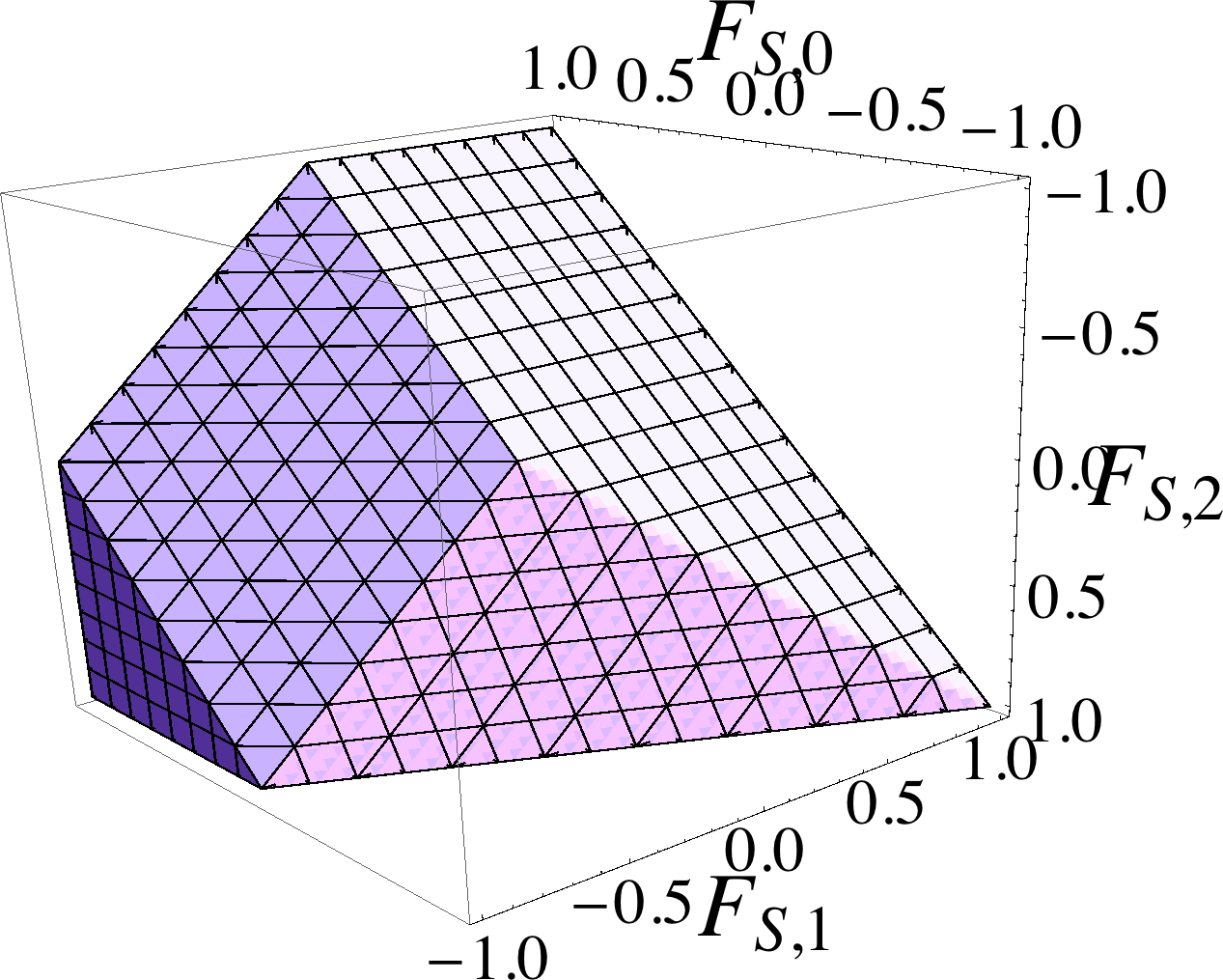
Figure 10: Positivity bound described by $M_{S}$, the linear conditions in the $S$-subspace. It is also the actual bound if new degrees of freedom only couple to longitudinal modes of SM gauge bosons.

The $M_{T}$ matrix contains 14 vectors. However, 3 of them are redundant as they can be written as positive linear combinations of the others. This can be seen by taking the 6 rows in $M_{T}$ with a $T_{\perp}$ polarisation. The corresponding conditions only involve the $F_{T,2}$, $F_{T,7}$ and $F_{T,9}$ coefficients. Similar to the first toy example discussed in Section 2, the $F_{T,2}$ component of these vectors is always positive, so we rescale these vectors so that the $F_{T,2}$ component is always equal to 1, and plot the 2nd and the 3rd components on a 2D plane, as in Figure 12. We see that the three channels involving a $Z$ boson correspond to points staying inside the triangle formed by the other three channels. Therefore, similar to the discussion in Section 3.1, the three vectors from $ZZ$, $WZ$ and $Z\gamma$ channels with a $T_{\perp}$ polarisation cannot lead to additional exclusion, and so we can remove them from $M_{T}$. They are labeled with $*$ in Eq. (218). One can check that the remaining 11 vectors form a convex pyramid, so it is not possible to further simplify $M_{T}$. The resulting constraint is then described by a pyramid with 11 edges in an 8-dimensional space.

The $M_{M}$ matrix contains 5 vectors, but only in a 3-dimensional space, spanned by $-2F_{M,1}+F_{M,7}$, $F_{M,3}$ and $F_{M,5}$. They already form a convex pyramid. Similar to Section 2, this can be seen by rescaling the vectors so that the $-2F_{M,1}+F_{M,7}$ component is always one, and plotting the remaining two components on a plane. We show this in Figure 12. Further simplification is not possible. The allowed parameter space is a pentagonal pyramid, shown in Figure 13.

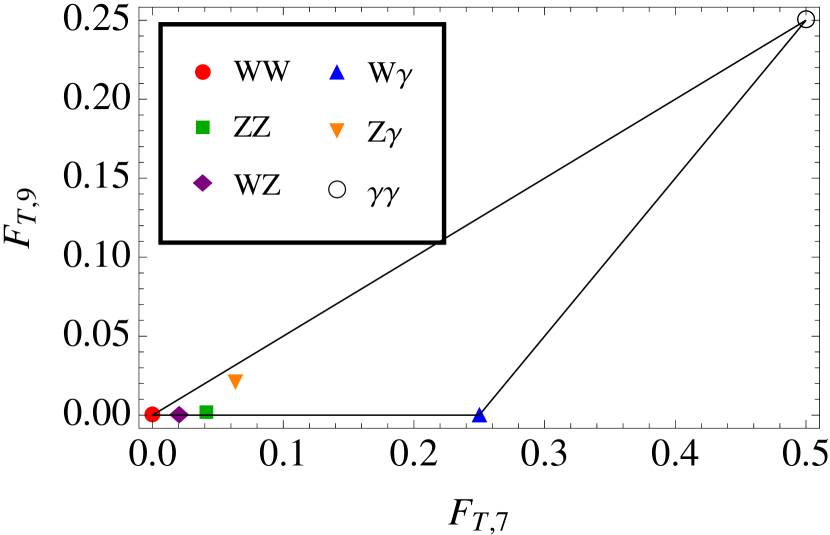
Figure 11: The 6 rows in $M_{T}$ with a $T_{\perp}$ polarisation only involve $F_{T,2}$, $F_{T,7}$ and $F_{T,9}$. The corresponding $\vec{x}_{i}$ vectors have 3 components. The plot shows the intersection points $P_{i}=(u,v)$ of $\vec{x}_{i}$ on the plane $(1,u,v)$. $P_{WZ}$, $P_{ZZ}$ and $P_{Z\gamma}$ are inside the triangle formed by $P_{WW}$, $P_{W\gamma}$ and $P_{\gamma\gamma}$.

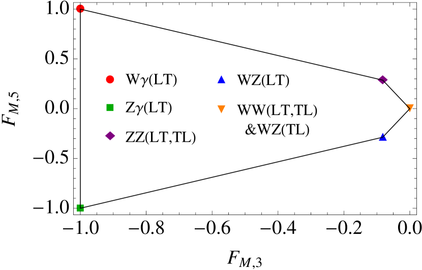
Figure 12: The 5 rows in $M_{M}$ only involve three parameters: $-2F_{M,1}+F_{M,7}$, $F_{M,3}$ and $F_{M,5}$. The corresponding $\vec{x}_{i}$ vectors have 3 components. The plot shows the intersection points $P_{i}=(u,v)$ of $\vec{x}_{i}$ on the plane $(1,u,v)$. We see that $P_{i}=(u,v)$ form a convex pentagon.

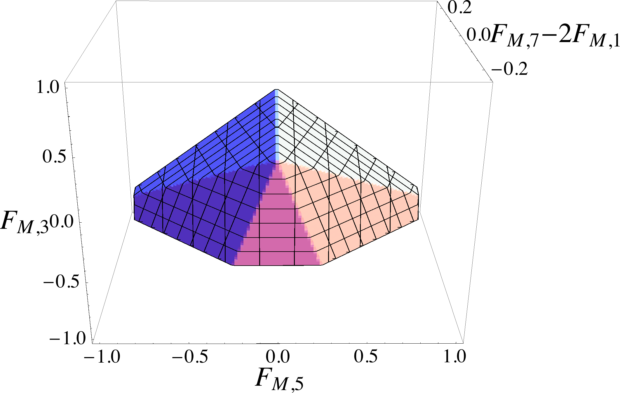
Figure 13: Positivity bound described by $M_{M}$, the linear conditions in the $M$-subspace.

As we have mentioned, if we consider a case where only the $M$-type operators are allowed, then quadratic conditions from $WW$ and $ZZ$ apply but they will be reduced to an additional set of linear conditions in the $M$ subspace, as shown in Eq. (230). For example, this is the case if the theory has a new vector field ${\mathcal{L}_{1}}$ which is a $SU(2)_{L}$ doublet, see Appendix A. In these special cases, we should also consider the additional linear conditions, which are described by the following matrix

$$\left(\begin{array}[]{ccccccc}4&-3&0&0&0&0&2\\ -4&-1&0&0&0&0&0\\ 4c_{W}^{4}&-2c_{W}^{4}&2s_{W}^{4}&-s_{W}^{4}&2s_{W}^{2}c_{W}^{2}&s_{W}^{2}c_{W}^{2}&c_{W}^{4}\\ -2c_{W}^{4}&0&-s_{W}^{4}&0&-s_{W}^{2}c_{W}^{2}&0&0\\ \end{array}\right)\begin{array}[]{l}WW,\bar{M}_{+-}\&\bar{M}_{\parallel}\\ WW,M_{+-}\&M_{\parallel}\\ ZZ,\bar{M}_{I}\\ ZZ,M_{I}\end{array}$$ (240)

With this matrix, two rows from $M_{M}$ can be removed: the $\vec{x}$ vector from $ZZ$ with $LT,TL$ polarisation is proportional to the sum of the $\vec{x}$ from the same channel but the $M_{I}$ and the $\bar{M}_{I}$ polarisation; the $\vec{x}$ vector from $WW$($ZZ$) channel with $LT,TL$($TL$) polarisation is proportional to the sum of the $\vec{x}$ from the $WW$ channel but with $M_{\parallel}$ and $\bar{M}_{\parallel}$ polarisation. Combining the two matrices and removing the two redundant rows gives a new matrix with 7 rows, which involve all $F_{M,i}$ operators. In addition, the quartic inequality from $WZ$ also applies, and it is reduced to a quadratic condition in the $M$ subspace, as in Eq. (231). To sum up, if the theory only generates $M$-type operators, the coefficients are constrained by 7 linear inequalities and 1 quadratic inequality.

To better understand the constraints in the $M$ subspace, it is useful to perform the following change of basis. Defining a set of new coefficients $C_{M,i}$ such that

$$M_{M,i}=R_{ij}C_{M,j}$$ (241)

where $R$ is given by

$$R=\left(\begin{array}[]{ccccccc}\frac{1}{24c_{W}^{2}}&-\frac{1}{24c_{W}^{2}}&0&1&-\frac{s_{W}^{4}}{2c_{W}^{4}}&\frac{1}{24c_{W}^{2}}&\frac{1}{48c_{W}^{2}}\\ -\frac{1}{6c_{W}^{2}}&\frac{1}{6c_{W}^{2}}&-\frac{1}{2c_{W}^{2}}&-4&0&-\frac{1}{6c_{W}^{2}}&-\frac{1}{12c_{W}^{2}}\\ 0&0&0&0&1&0&-\frac{c_{W}^{2}}{8s_{W}^{4}}\\ 0&-\frac{c_{W}^{2}}{s_{W}^{4}}&\frac{c_{W}^{2}}{s_{W}^{4}}&0&0&0&0\\ \frac{5}{12s_{W}^{2}}&-\frac{5}{12s_{W}^{2}}&0&\frac{4c_{W}^{2}}{s_{W}^{2}}&0&-\frac{1}{12s_{W}^{2}}&\frac{1}{12s_{W}^{2}}\\ -\frac{1}{s_{W}^{2}}&\frac{1}{s_{W}^{2}}&0&0&0&0&0\\ -\frac{1}{3c_{W}^{2}}&\frac{1}{3c_{W}^{2}}&0&-8&0&-\frac{1}{3c_{W}^{2}}&-\frac{1}{6c_{W}^{2}}\\ \end{array}\right)$$ (249)

Then the 7 linear conditions in the $M$ space can be written as

$$M^{\prime}_{M,ij}C_{M,j}>0,$$ (250)

$$M^{\prime}_{M}=\left(\begin{array}[]{cccccccc}1&0&0&0&0&0&0\\ -s_{W}^{2}&1&s_{W}^{2}/c_{W}^{2}-1&0&0&0&0\\ s_{W}^{2}&c_{W}^{2}-s_{W}^{2}&s_{W}^{2}/c_{W}^{2}-1&0&0&0&0\\ 0&0&3c_{W}^{2}&0&-4s_{W}^{4}&0&0\\ 0&0&c_{W}^{2}&0&4s_{W}^{4}&0&0\\ 0&1&0&12c_{W}^{2}&0&0&0\\ -1&1&0&-12c_{W}^{2}&0&0&0\\ \end{array}\right)\begin{array}[]{l}WZ,LT\\ W\gamma,LT\\ Z\gamma,LT\\ WW,\bar{M}_{+-}\&\bar{M}_{\parallel}\\ WW,M_{+-}\&M_{\parallel}\\ ZZ,\bar{M}_{I}\\ ZZ,M_{I}\end{array}$$ (265)

and the quadratic condition from $WZ$ is simply $4C_{M,1}C_{M,3}>C_{M,6}^{2}$. We can see that $C_{M,7}$ is a free parameter that is not constrained. This is the only degree of freedom that is free in the full 18-dimensional parameter space. For the rest of the conditions, the 7 linear ones form a pyramid with 7 edges in a 5-dimensional subspace, while the quadratic condition carves out a cone in a 3-dimensional subspace that involves the 6th direction and is partially orthogonal to the pyramid. It is difficult to display the shape, but a parameter scan can be easily performed in this basis. Let

$$C_{M,1},C_{M,3}\in[0,+\infty)$$ (266)

vary freely. Then $C_{M,2}$ is bounded from below by the 2nd, the 3rd, and the combination of the last two linear conditions:

$$C_{M,2}>\max\left(s_{W}^{2}C_{M,1}+\frac{c_{W}^{2}-s_{W}^{2}}{c_{W}^{2}}C_{M,3},-\frac{s_{W}^{2}}{c_{W}^{2}-s_{W}^{2}}C_{M,1}+\frac{1}{c_{W}^{2}}C_{M,3},\frac{1}{2}C_{M,1}\right)$$ (267)

Then the rest coefficients are bounded by the above three from both sides:

$$C_{M,4}\in\left(-\frac{1}{12c_{W}^{2}}C_{M,2},\frac{1}{12c_{W}^{2}}\left(C_{M,2}-C_{M,1}\right)\right)$$ (268)

$$C_{M,5}\in\left(-\frac{c_{W}^{2}}{4s_{W}^{4}}C_{M,3},\frac{3c_{W}^{2}}{4s_{W}^{4}}C_{M,3}\right)$$ (269)

$$C_{M,6}\in\left(-2\sqrt{C_{M,1}C_{M,3}},2\sqrt{C_{M,1}C_{M,3}}\right)$$ (270)

4.2 Cones

Now let us focus on the quadratic conditions. These conditions typically have the following form

$$4xy>\max(0,z_{1},z_{2})^{2}$$ (271)

where $x$ and $y$ are linear combinations of $S$ and $T$ operator coefficients respectively, and $z_{1,2}$ are linear combinations of $M$ coefficients. The shape of this constraint can be fully seen only when we turn on three different types of operators simultaneously. Since $x>0$ and $y>0$ are always included in the linear conditions, this condition can be considered as the intersection of two constraints:

$$2\sqrt{xy}>z_{1}\quad\mbox{and}\quad 2\sqrt{xy}>z_{2}$$ (272)

A constraint like $2\sqrt{xy}>z$ is trivial for a negative $z$, while for a positive $z$ it gives a half cone:

$$u^{2}-v^{2}>z^{2},\ z>0$$ (273)

$$\mbox{where}\ u\equiv x+y\ \mbox{and}\ v\equiv x-y$$ (274)

As an example, consider the first quadratic condition from $WW$, in the subspace spanned by $F_{S,1}$, $F_{M,1}$ and $F_{T,1}$:

$$32F_{S,1}F_{T,1}>\max(0,3F_{M,1},F_{M,1})^{2}=\left\{\begin{array}[]{ll}0&F_{M,1}<0\\ 9F_{M,1}^{2}&F_{M,1}>=0\end{array}\right.$$ (277)

We show this constraint in Figure 15. It is a combination of a triangular pyramid and a half cone.

Figure 14: Positivity bound from the quadratic inequality in the $WW$ channel, in the subspace spanned by $F_{S,1}$, $F_{M,1}$ and $F_{T,1}$.

Figure 15: Same as Figure 15, but in the subspace spanned by $F_{S,1}$, $F_{M,0}$ and $F_{T,1}$.

Sometimes the bounds from $z_{1}$ and $z_{2}$ combine to form a full cone. This is the case for e.g. $F_{S,1}$, $F_{M,0}$ and $F_{T,1}$,

$$2F_{S,1}F_{T,1}>\max(0,-F_{M,0},F_{M,0})^{2}=F_{M,0}^{2}$$ (278)

The corresponding bound is shown in Figure 15, which is now symmetric on both sides. It is also possible that the two sides of the cone are not symmetric. Consider a case where we impose a restriction $F_{M,0}+F_{M,1}=0$, then the quadratic condition becomes:

$$32F_{S,1}F_{T,1}>\max(0,3F_{M,0},-7F_{M,0})^{2}$$ (279)

We show this “asymmetric cone” in Figure 17.

Figure 16: Similar to Figure 15, but imposing a restriction $F_{M,0}+F_{M,1}=0$.

Figure 17: Similar to Figure 15, but imposing a restriction $F_{M,1}=-1/2$.

The full structure of the bound, described Eq. (271), become manifest only in a 4-dimensional space, because in general $z_{1}$ and $z_{2}$ are linearly independent. Consider the subspace spanned by $F_{S,0}$, $F_{M,0}$, $F_{M,1}$ and $F_{T,1}$. The condition becomes

$$32F_{S,1}F_{T,1}>\max(0,4F_{M,0}+F_{M,1},-4F_{M,0}+3F_{M,1})^{2}$$ (280)

It is not possible to make a 4D plot. However, to visualize this, we can write the boundary as:

$$\max(0,4F_{M,0}+F_{M,1},-4F_{M,0}+3F_{M,1})=4w$$ (281)

$$\sqrt{2F_{S,1}F_{T,1}}=w$$ (282)

and make contour plots for $w$ in the $F_{M,0}-F_{M,1}$ space and the $F_{S,1}-F_{T,1}$ space. These two plots are shown in Figure 18. The second contour plot describes a half cone, where $w$ is a direction perpendicular to its axis. The first one tells us that the constraint is the intersection of two half cones, with their $w$ directions pointing to the $F_{M,0}=4F_{M,1}$ direction and to the $F_{M,0}=-\frac{4}{3}F_{M,1}$ direction, respectively. Furthermore, in Figure 18 left, if we take the green, the red and the blue axes separately and make a 3-D plot together with $F_{S,0}$ and $F_{S,1}$, we will get the shapes of a half-cone, a symmetric cone and an asymmetric cone, which explains Figures 15, 15 and 17. We could also consider the orange axis which goes off the origin, $F_{M,1}=-1/2$. This will lead to the shape in Figure 17, with a plateau between two half cones.

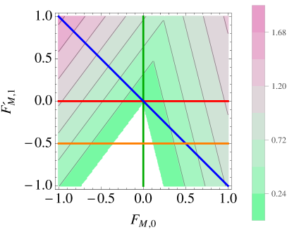
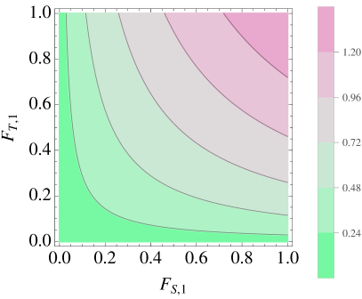
Figure 18: Contour plots for Eqs. (281) and (282), which describes the quadratic inequality from the $WW$ channel, in the subspace of $F_{S,1}$, $F_{T,1}$, $F_{M,0}$ and $F_{M,1}$.

The other quadratic constraints from $WW$ and $ZZ$ have similar forms, so we do not discuss them separately. The one from $WZ$ is more complicated, as the terms in the $\max$ function involve additional square roots. This inequality describes a 5-dimensional object. In Figure 19, we show it in the space of $F_{S,0}$, $F_{T,1}$, $F_{M,1}$, $F_{M,3}$, and $F_{M,4}$, by plotting the first four coefficients in a similar way as in Figure 18, but for different values of $F_{M,4}$, .

Figure 19: Similar to Figure 18, but for the quartic inequality from the $WZ$ channel, in the subspace of $F_{S,0}$, $F_{T,1}$, $F_{M,1}$ and $F_{M,3}$, with different values of $F_{M,4}$.

5 Volumes of allowed parameter spaces

While the shapes of the bounds describe the relations between different parameters, their constraining power is more reflected by the volume of the allowed higher-dimensional parameter space. For example, Ref. Durieux:2017rsg proposed to use the GDP parameter to assess the overall strength of a $n$-dimensional constraint, which is proportional to the $n$th root of the volume of the constrained parameter space.

However, this is not a useful measure for the problem at hand, because the positivity conditions only constrain the possible directions in which the deviation could occur, so the volume in the regular sense is always infinity. For this reason, we define the “volume” of the constraint by the solid angle spanned by the allowed parameter space. They can be easily computed in a Monte Carlo approach. A random vector of coefficients $\vec{F}=(F_{S,0},F_{S,1},\cdots)$ can be generated by combining 18 independent random numbers under the Gaussian distribution, and normalizing them so that the magnitude is equal to one. Vectors generated in this way are uniformly distributed on a unit sphere in the 18-D parameter space. With a random vector $\vec{F}$ we can check explicitly if a certain positivity condition is satisfied. By generating many of these vectors, we can count the fraction of the ones that satisfy this condition. In the rest of this section, we will refer to this fraction as the volume of the parameter space allowed by a given positivity condition, and we denote it by $V$. Of course, the volume defined in this way depends on the relative rescaling of operators, and needs to be interpreted with a grain of salt.

The linear conditions form 3 pyramids in 3 subspaces, $S$, $M$ and $T$, that are completely orthogonal to each other, so their volumes can be computed separately. We find that

$$V_{S}=0.38,\quad V_{M}=0.34,\quad V_{T}=0.16$$ (283)

and all together they constrain the full parameter space to

$$V_{S}V_{M}V_{T}=0.022$$ (284)

i.e. 2.2% of the full parameter space. In other words, the linear conditions solely are sufficient to reduce the full parameter space by two orders of magnitude.

We have mentioned that there are two linear inequalities derived from $WW$ channel that require complex polarisation. If we restrict to only real polarisation, the $T$ subspace will have a slightly weaker constraining power, which leads to $V_{T,real}=0.17$. The size of the total constraint will become 0.023.

	$WW$ 1st	$WW$ 2nd	$ZZ$	$WZ$	All
Volume	0.20	0.22	0.20	0.12	0.05
Improvement	12%	$\approx$0%	10%	64%	94.5%

Table 2: The volume of parameter space allowed by each quadratic and quartic positivity condition, together with the corresponding improvement when all other bounds are turned on. “All” is the combination of all quadratic and quartic conditions.

Now let us consider the quadratic and quartic conditions. There are two from $WW$, one from $ZZ$, and one from $WZ$. In Table 2, the first row gives the volume of each condition, while the second line gives the corresponding improvement due to this condition. The latter is defined by comparing two volumes: $V_{total}$ which is volume of the combination of all quadratic and quartic conditions, and $V_{remove}$ which is the volume of the combination of all conditions except for one that is removed. The improvement is defined as $1-V_{total}/V_{remove}$, which gives us an idea of how useful a specific bound is, in the presence of all other bounds. From the table we see that the constraining power of each quadratic or quartic one is quite good, but they are not orthogonal to each other, so the volume of all conditions combined are weaker than the linear case, at about 5% of the total parameter space. In particular, from the second row we can see that once three conditions are taken into account, the last one does not improve much except for $WZ$. The second condition from $WW$ almost leads to no improvement. We checked that this improvement is not strictly zero, so the condition is still an independent one, but the size of the improvement only shows up in the second digit after the decimal point. This means that most part of the parameter space allowed by the other three constraints automatically satisfies this condition.

	S	M	T	$WW$ 1st	$WW$ 2nd	$ZZ$	$WZ$	All
Volume	0.38	0.34	0.16	0.20	0.22	0.20	0.12	0.021
Improvement	0	27%	49%	1.1%	$\approx$0%	2.5%	0.1%	97.9%

Table 3: Similar to Table 2, but for all linear, quadratic and quartic conditions. The S, M, and T column represent the linear conditions in $S$-, $M$- and $T$-subspaces, while the next four columns represent quadratic and quartic conditions as in Table 2.

Finally in Table 3, we show a similar table but including both linear and quadratic conditions. The first line compares the volumes of each condition. The volume of all conditions together is 2.1% of the total, only slightly better than the case of linear conditions only, which is 2.2%. So even though the quadratic conditions themselves could carve out a parameter space with a volume of only 5%, the impact is tiny once the linear conditions are already taken into account. In the second row we show the improvements of each condition. As expected we see that the improvements due to the quadratic and quartic conditions are small. The linear conditions in the $S$ subspace lead to no improvement, because the three corresponding linear inequalities are required to define the quadratic/quartic conditions from $WW$, $ZZ$ and $WZ$ respectively. Finally, if we only use real polarisation, the volume of the total constraint is 2.3%.

6 Positivity bounds for one, two, and three operators

From the SMEFT point of view, the most useful and correct bounds are the global ones, obtained with all relevant EFT operators switched on. However, studying lower dimensional subspace of the full parameter space is always illustrative. It could help to understand for example the constraining power on certain directions, or correlations between different parameters. In addition, in VBS studies, experimental limits have been presented only in terms of individual or at most two-dimensional bounds, even though more global analyses can be foreseen in the future.

To better understand the positivity constraints in lower dimensional parameter space, and to facilitate a quick comparison with the current experimental results, in this section we will explicitly list the positivity bounds with one, two or three operators switched on at a time. These results could also be used as a guidance for future searches.

6.1 One operator at a time

We first consider the case where only one operator is nonzero. This is the easiest way to see the impact of positivity, as it can be directly confronted with experimental limits, most of which are presented as individual limits qgclimits . In Table 4, we list the positivity constraints on all individual operators. In particular, $F_{T,5},F_{T,7},F_{M,0},F_{M,2},F_{M,4},F_{M,5}$ cannot individually take any nonzero value. Individual limits on these operators do not have a clear meaning, because there is no UV completion that can generate any of these operators alone. All other coefficients are constrained to have a certain sign, either positive or negative, and so their individual bounds could have been presented as one-sided limits.

$F_{S,0}$	$F_{S,1}$	$F_{S,2}$	$F_{M,0}$	$F_{M,1}$	$F_{M,2}$	$F_{M,3}$	$F_{M,4}$	$F_{M,5}$
+	+	+	✗	$-$	✗	$-$	✗	✗
$F_{M,7}$	$F_{T,0}$	$F_{T,1}$	$F_{T,2}$	$F_{T,5}$	$F_{T,6}$	$F_{T,7}$	$F_{T,8}$	$F_{T,9}$
+	+	+	+	✗	+	✗	+	+

Table 4: Positivity constraints on individual VBS operator coefficients. $+/-$ means the coefficient must be non-negative or non-positive. ✗ means that nonzero value is not allowed.

6.2 Two operators at a time

Two-operator constraints have been presented for example in Refs. CMS:2018ysc ; Khachatryan:2014sta ; Aad:2014zda . Since all positivity inequalities are homogeneous polynomials, they always carve out triangle areas in the 2D parameter spaces.

Consider the three types of operators: $S$-type, $M$-type and $T$-type. When only two operators are turned on, there is no correlation between operators from two different categories. This is obvious for the linear conditions in Eqs. (178), (189) and (218). To see that this is also true for higher order inequalities, we note that both quadratic and quartic inequalities can be written in the form of

$$f(F_{S,i})g(F_{T,i})>\max(0,h_{1}(F_{M,i}),h_{2}(F_{M,i}))^{2}$$ (285)

where $f$, $g$ and $h_{1,2}$ are homogeneous functions of degree 1. If $M$-type operator is not turned on, the r.h.s. is 0 and so the inequality is trivial. If a $M$-type operator is turned on with another $S$-type or $T$-type operator, the l.h.s. is 0 and so the inequality reduces to $h_{1,2}(F_{M,i})<0$. In either case there is no correlation across different types. This means that we only need to show bounds for operator pairs from the same category. For those from different ones, one can simply refer to Table 4.

These 2D bounds are shown in Figures 20, 21, and 22. The exact description of the bounds are given in Appendix B, together with the corresponding polarisation configuration.

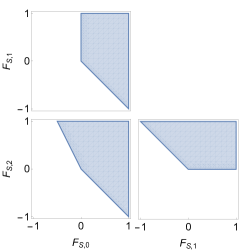
Figure 20: Positivity constraints on all $F_{S,i}$ pairs.

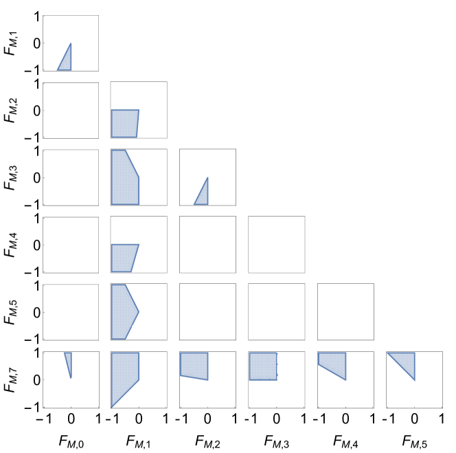
Figure 21: Positivity constraints on all $F_{M,i}$ pairs.

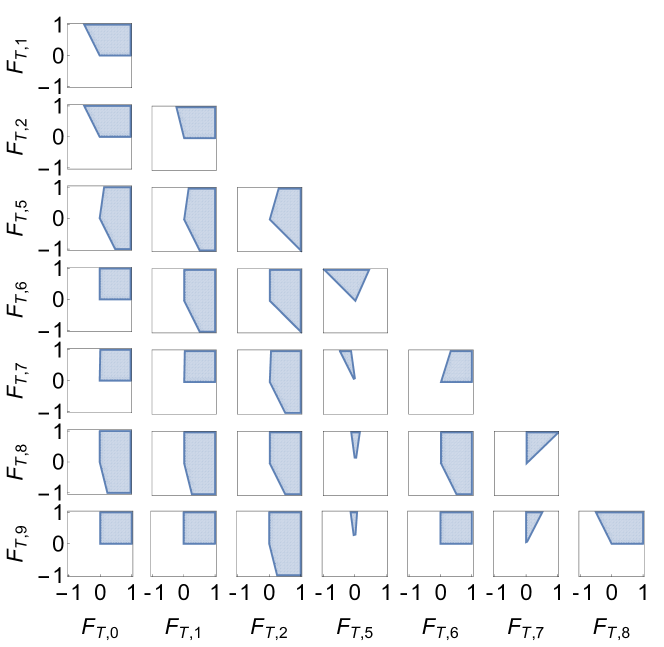
Figure 22: Positivity constraints on all $F_{T,i}$ pairs.

6.3 Three operators at a time

When three operators are turned on simultaneously, the linear conditions continue to carve out pyramids in each $S$-, $M$-, and $T$-subspaces. The higher order ones could potentially carve out cones or half cones, as discussed in Section 4.2. The correlation across different types of operators could appear, but only if one turns on one $S$, one $M$, and one $T$ operator simultaneously. The shape of bound depends on which types of operators are turned on.

• If we turn on three operators in the same category, the situation has been discussed already in Section 4.1. The $S$ and $T$-subspaces are constrained by pyramids or prisms, while the $M$-subspace by a pyramid and/or a cone, depending on whether the chosen operators can probe the cone in the $C_{M,1}$, $C_{M,3}$ and $C_{M,6}$ subspace. For example, choosing $(F_{M,0},F_{M,1},F_{M,2})$ gives a pyramid, while $(F_{M,3},F_{M,5},F_{M,7})$ gives a cone.

• If we turn on operators that belong to two different categories, similar to the two-operator case, there is again no correlation between the two categories. The bounds are then reduced to individual bound in one category and 2D bounds in another, which have all been discussed in the previous two subsections.

• Finally, if we consider three operators that belong to three different types, the quadratic and quartic bounds cannot be decomposed into individual category. They will potentially carve out cones or half cones as discussed in Section 4.2.

Due to the large number of possible combinations, here we only list some representative cases in Figures 23, 24, 25, and 26. The corresponding boundaries are described in Appendix C, together with polarisation conditions.

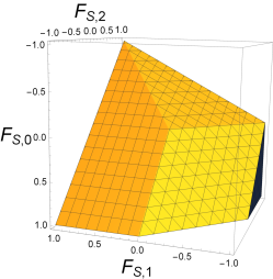
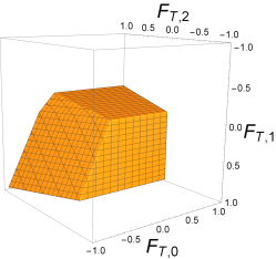
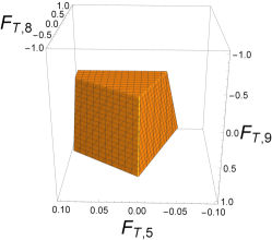
Figure 23: Representative cases for three $S$-type or three $T$-type operators. Allowed parameter spaces are described by pyramids.

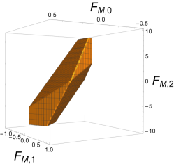
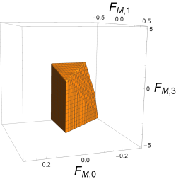
Figure 24: Representative cases for three $M$-type operators. Allowed parameter spaces are described by pyramids.

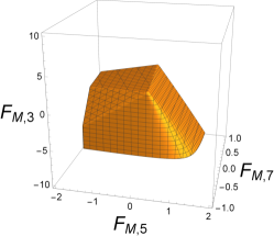
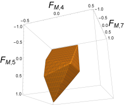
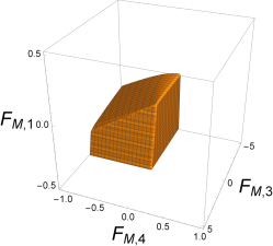
Figure 25: Representative cases for three $M$-type operators. Allowed parameter spaces are described by combining a pyramid and a cone.

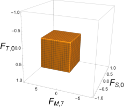
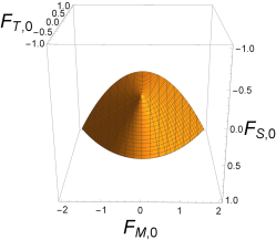
Figure 26: Representative cases for operators from three different categories. Allowed parameter spaces are described by a pyramid or a cone.

7 Summary

Searching for deviations in QGC couplings is one of the main goals of the electroweak program at the LHC. We have shown that a set of theoretical bounds on anomalous QGC couplings can be derived, by requiring that the scattering amplitudes of specific VBS channels with specific polarisation states satisfy the fundamental principles of the quantum field theory. While these bounds do not constrain the magnitude of possible deviations from the SM, they constrain the possible directions in the 18-dimensional QGC parameter space in which SM deviations may be observed at all. Therefore they have important implications on future studies.

We have solved these positivity constraints and removed the dependence on the polarisation of external particles. The exact parameter space which satisfies all positivity conditions is described by a set of most crucial polarisation states: once positivity bounds are satisfied for these states, they are guaranteed to be satisfied for any other polarisation. The bounds derived from these polarisation states can be easily used to guide future experimental searches, to optimise the parameter scan, and to improve the presentation of resulting limits. They also help future theoretical studies based on the EFT formalism in a bottom-up way, to choose reasonable benchmark scenarios. We have then studied the shapes and the volumes of these bounds. To understand how these constraints may arise from the underlying model point of view, we have considered a simplified model with several new resonant states coupled to SM electroweak gauge bosons, and showed that the positivity bounds are indeed satisfied by the corresponding EFT.

The most important results are summarised below:

• The positivity condition on coefficients $\vec{F}$, from channel $i$ and external polarisation $\vec{a}$ and $\vec{b}$, is described by $\vec{F}\cdot\vec{x}_{i}(\vec{a},\vec{b})>0$, where the vector $\vec{x}_{i}(\vec{a},\vec{b})$ can be computed from $f^{q_{1}q_{2}}_{ab,\epsilon\Lambda}(s)$. For arbitrary complex $\vec{a}$ and $\vec{b}$, we identify the boundaries of the set of $\vec{x}_{i}(\vec{a},\vec{b})$, which fully characterise the allowed parameter space independent of $\vec{a}$ and $\vec{b}$. They are described by 19 linear inequalities, 3 quadratic inequalities, and 1 quartic inequality, given in Eqs. (107), (108), (109), (119), (120), (130), (131), (143), (144) and (145).

• The $S$-type, $M$-type of $T$-type operator coefficients form 3 subspaces. The 19 linear positivity constraints are decoupled into these 3 subspaces, with no correlation across. These linear constraints then describe the direct product of a pyramid in the $S$-space, one in the $T$-space, and a prism in the $M$-space. Altogether, this reduces the allowed parameter space to 2.2% of the total, in terms of solid angle.

• The quadratic and quartic bounds always involve all three subspaces. They can be written in the form of

  $$f(F_{S,i})g(F_{T,i})>\max(0,h_{1}(F_{M,i}),h_{2}(F_{M,i}))^{2}$$ (286)

  where $f$, $g$ and $h_{1,2}$ are homogeneous functions of degree 1. They carve out (approximately) half cones in the parameter space. Together, they can reduce the parameter space to 5% of the total. When combined with the linear constraints, they only slightly improve the parameter space to 2.1%.

• In UV completions where new degrees of freedom dominantly couple to the longitudinal modes of electroweak gauge bosons, positivity bounds carve out a 3-dimensional triangular pyramid in the $S$-space.

• In UV completions where new degrees of freedom dominantly couple to the transversal modes of electroweak gauge bosons, the constraint is described by a pyramid with 11 edges in the 8-dimensional $T$-space.

• In UV completions where new degrees of freedom couple to both modes, but only generate $M$-type operators, the constraint in the 7-dimensional $M$-space is the intersection of a pyramid with 7 edges in a 5-dimensional subspace and a cone in a 3-dimensional subspace that involves the 6th direction and is partially orthogonal to the pyramid. The 7th direction is unconstrained.

• For the convenience of future QGC studies, we have presented the complete descriptions of all 1-D and 2-D subspaces, i.e. constraints on all individual operators and all pairs of operators. We have also shown examples of 3-D subspaces.

Appendix A Simplified models

Inspired by the simplified model in Ref. Brass:2018hfw , we extend the SM by adding new particles that coupled to the longitudinal and/or the transversal modes of the electroweak gauge bosons. Following the notation of Ref. deBlas:2017xtg , we consider four possible new fields. Their names and irreducible representations under $SU(3)_{C}\times SU(2)_{L}\times U(1)_{Y}$ are given in Table 5.

Names	scalar ${\mathcal{S}}$	scalar ${{\Xi}}$	scalar ${{\Xi}_{1}}$	vector ${\mathcal{L}_{1}}$
Irrep	$(1,1)_{0}$	$(1,3)_{0}$	$(1,3)_{1}$	$(1,2)_{\frac{1}{2}}$

Table 5: New particles in the simplified model that we consider as examples of UV completion.

The Lagrangian of the simplified model can be split into two pieces

$$\mathcal{L}_{BSM}=\mathcal{L}_{kin}+\mathcal{L}_{int}$$ (287)

The kinematic terms are standard:

$$\mathcal{L}_{kin}= \frac{1}{2}D_{\mu}{\mathcal{S}}D^{\mu}{\mathcal{S}}-\frac{1}{2}M_{\mathcal{S}}^{2}{\mathcal{S}}^{2}+\frac{1}{2}D_{\mu}{{\Xi}}^{i}D^{\mu}{{\Xi}}^{i}-\frac{1}{2}M_{{\Xi}}^{2}{{\Xi}}^{i}{{\Xi}}^{i}$$

$$+\left(D_{\mu}{{\Xi}_{1}}^{i}\right)^{\dagger}D^{\mu}{{\Xi}_{1}}^{i}-M_{{\Xi}_{1}}^{2}{{{\Xi}_{1}}^{i}}^{\dagger}{{\Xi}_{1}}^{i}$$

$$+\left(D_{\mu}{\mathcal{L}_{1}}_{\nu}\right)^{\dagger}D^{\nu}{\mathcal{L}_{1}}^{\mu}-\left(D_{\mu}{\mathcal{L}_{1}}_{\nu}\right)^{\dagger}D^{\mu}{\mathcal{L}_{1}}^{\nu}+M_{\mathcal{L}_{1}}^{2}{\mathcal{L}_{1}}^{\mu\dagger}{\mathcal{L}_{1}}_{\mu}\,.$$ (288)

The interaction terms can be written as

$$\mathcal{L}_{int}= {\mathcal{S}}{\mathcal{J}}_{\mathcal{S}}+{{\Xi}}^{i}{\mathcal{J}}_{{\Xi}}^{i}+\left({{{\Xi}_{1}}^{i}}^{\dagger}{\mathcal{J}}_{{\Xi}_{1}}^{i}+h.c.\right)+\left({{\mathcal{L}_{1}}^{\mu}}^{\dagger}{{\mathcal{J}}_{\mathcal{L}_{1}}}_{\mu}+h.c.\right)$$ (289)

and the currents are

$${\mathcal{J}}_{\mathcal{S}}=a_{H}\left(D_{\mu}\phi\right)^{\dagger}D^{\mu}\phi+a_{W}W_{\mu\nu}^{i}W^{i\mu\nu}+a_{B}B_{\mu\nu}B^{\mu\nu}$$ (290)

$${\mathcal{J}}_{{\Xi}}^{i}=b_{H}\left(D_{\mu}\phi\right)^{\dagger}\sigma^{i}D^{\mu}\phi+b_{WB}W^{i}_{\mu\nu}B^{\mu\nu}$$ (291)

$${\mathcal{J}}_{{\Xi}_{1}}^{i}=c_{H}\left(D_{\mu}\tilde{\phi}\right)^{\dagger}\sigma^{i}D_{\mu}\phi$$ (292)

$${\mathcal{J}}_{\mathcal{L}_{1}}^{\mu}=d_{HB}D_{\nu}\phi B^{\nu\mu}+d_{HW}\sigma^{i}D_{\nu}\phi W^{i\nu\mu}$$ (293)

where $i$ is the $SU(2)_{L}$ triplet index. $\tilde{\phi}\equiv i\sigma^{2}\phi^{*}$. $a_{i},b_{i},c_{i},d_{i}$ are coupling strengths. By solving the equation of motion for the heavy fields, and plugging them back into the Lagrangian, we find that up to the dimension-8, the effective Lagrangian can be written as

$$\mathcal{L}=\frac{1}{2}M_{\mathcal{S}}^{-2}{\mathcal{J}}_{\mathcal{S}}^{2}+\frac{1}{2}M_{{\Xi}}^{-2}{\mathcal{J}}_{{\Xi}}^{i}{\mathcal{J}}_{{\Xi}}^{i}+M_{{\Xi}_{1}}^{-2}{{\mathcal{J}}_{{\Xi}_{1}}^{i}}^{\dagger}{\mathcal{J}}_{{\Xi}_{1}}^{i}-M_{\mathcal{L}_{1}}^{-2}{{\mathcal{J}}_{\mathcal{L}_{1}}^{\mu}}^{\dagger}{\mathcal{J}}_{{\mathcal{L}_{1}}\mu}$$ (294)

With this we can write down the coefficients of the 18 QGC operators.

$$\begin{aligned} &F_{S,0}=2\frac{c_{H}^{2}}{M_{{\Xi}_{1}}^{2}}\\ &F_{S,1}=\frac{a_{H}^{2}}{2M_{\mathcal{S}}^{2}}-\frac{b_{H}^{2}}{2M_{{\Xi}}^{2}}\\ &F_{S,2}=\frac{b_{H}^{2}}{M_{{\Xi}}^{2}}\\ &F_{T,0}=\frac{\bar{a}_{W}^{2}}{2M_{\mathcal{S}}^{2}}\\ &F_{T,5}=\frac{\bar{a}_{W}\bar{a}_{B}}{M_{\mathcal{S}}^{2}}\\ &F_{T,6}=\frac{\bar{b}_{WB}^{2}}{M_{{\Xi}}^{2}}\\ &F_{T,8}=\frac{\bar{a}_{B}^{2}}{2M_{\mathcal{S}}^{2}}\end{aligned}\quad\begin{aligned} &F_{M,0}=\frac{a_{H}\bar{a}_{W}}{M_{\mathcal{S}}^{2}}\\ &F_{M,1}=-\frac{\bar{d}_{HW}^{2}}{M_{\mathcal{L}_{1}}^{2}}\\ &F_{M,2}=\frac{a_{H}\bar{a}_{B}}{M_{\mathcal{S}}^{2}}\\ &F_{M,3}=-\frac{\bar{d}_{HB}^{2}}{M_{\mathcal{L}_{1}}^{2}}\\ &F_{M,4}=2\frac{b_{H}\bar{b}_{WB}}{M_{{\Xi}}^{2}}\\ &F_{M,5}=2\frac{\bar{d}_{HW}\bar{d}_{HB}}{M_{\mathcal{L}_{1}}^{2}}\\ &F_{M,7}=-\frac{\bar{d}_{HW}^{2}}{M_{\mathcal{L}_{1}}^{2}}\end{aligned}$$ (295)

where for convenience we have defined:

$$\bar{a}_{W}=-2g^{-2}a_{W},\qquad\bar{a}_{B}=-4g^{\prime-2}a_{B},$$ (296)

$$\bar{b}_{WB}=-2g^{-1}g^{\prime-1}b_{WB},\qquad\bar{d}_{HW}=2g^{-1}d_{HW},\qquad\bar{d}_{HB}=2g^{\prime-1}d_{HB}\,.$$ (297)

The coefficients which are not included above vanish in this model.

Note that this simplified model itself is not a UV completed theory. The interaction terms in Eq. (289) are of mass dimension five, so they need to be UV completed above some energy scale. However, at the tree level we expect the positivity condition to be satisfied. This is because for dim-5 interactions we expect the amplitude to grow like $\mathcal{O}(s)$ at large $s$, which already satisfies the Froissart-Martin bound. This is one of the main requirements to derive positivity bounds. The others such as analyticity and Lorentz invariance are trivially satisfied in this model.

To see explicitly how the positivity is satisfied, we first check the linear conditions. Plugging in Eq. (295) to the linear inequalities (178)–(218), we find

$$M_{S}\cdot F_{S}=\left(\begin{array}[]{c}\frac{1}{2}\left(\frac{a_{H}^{2}}{M_{\mathcal{S}}^{2}}+\frac{b_{H}^{2}}{M_{{\Xi}}^{2}}+\frac{8c_{H}^{2}}{M_{{\Xi}_{1}}^{2}}\right)\\ \frac{1}{2}\left(\frac{a_{H}^{2}}{M_{\mathcal{S}}^{2}}+\frac{b_{H}^{2}}{M_{{\Xi}}^{2}}+\frac{4c_{H}^{2}}{M_{{\Xi}_{1}}^{2}}\right)\\ \frac{b_{H}^{2}}{M_{{\Xi}}^{2}}+\frac{2c_{H}^{2}}{M_{{\Xi}_{1}}^{2}}\\ \end{array}\right)\,,$$ (301)

$$M_{T}\cdot F_{T}=\left(\begin{array}[]{c}0\\ 0\\ \frac{a_{W}^{2}}{M_{\mathcal{S}}^{2}}\\ \frac{4a_{W}^{2}}{M_{\mathcal{S}}^{2}}\\ \frac{(a_{B}s_{W}^{4}+2a_{W}c_{W}^{4})^{2}}{M_{\mathcal{S}}^{2}}+\frac{4b_{WB}^{2}s_{W}^{4}c_{W}^{4}}{M_{{\Xi}}^{2}}\\ 0\\ 0\\ \frac{4b_{WB}^{2}s_{W}^{4}}{M_{{\Xi}}^{2}}\\ 0\\ \frac{4b_{WB}^{2}}{M_{{\Xi}}^{2}}\\ 0\\ \frac{4b_{WB}^{2}\left(c_{W}^{2}-s_{W}^{2}\right)^{2}}{M_{{\Xi}}^{2}}+\frac{4\left(a_{B}s_{W}^{2}-2a_{W}c_{W}^{2}\right)^{2}}{M_{\mathcal{S}}^{2}}\\ 0\\ \frac{(a_{B}+2a_{W})^{2}}{M_{\mathcal{S}}^{2}}+\frac{4b_{WB}^{2}}{M_{{\Xi}}^{2}}\\ \end{array}\right)\,,$$ (316)

$$M_{M}\cdot F_{M}=\left(\begin{array}[]{c}\frac{2d_{HW}^{2}}{M_{\mathcal{L}_{1}}^{2}}\\ \frac{d_{HW}^{2}c_{W}^{4}+\left(d_{HW}c_{W}^{2}+d_{HB}s_{W}^{2}\right)^{2}}{M_{\mathcal{L}_{1}}^{2}}\\ \frac{d_{HW}^{2}c_{W}^{4}+\left(d_{HW}c_{W}^{2}-d_{HB}s_{W}^{2}\right)^{2}}{M_{\mathcal{L}_{1}}^{2}}\\ \frac{2d_{HW}^{2}}{M_{\mathcal{L}_{1}}^{2}}\\ \frac{\left(d_{HB}+d_{HW}\right)^{2}+d_{HW}^{2}}{M_{\mathcal{L}_{1}}^{2}}\\ \frac{\left(d_{HB}-d_{HW}\right)^{2}+d_{HW}^{2}}{M_{\mathcal{L}_{1}}^{2}}\\ \end{array}\right)\,.$$ (323)

The r.h.s. are always sums of squared terms, which are positive definite, so the linear positivity conditions are indeed satisfied.

To see that the quadratic conditions are satisfied, we randomly generate the coupling strengths in the range $-1\sim 1$ TeV^-1 and masses in the range $1\sim 2$ TeV, and plot the corresponding parameter space. For example, the first quadratic condition from the $WW$ channel is $4f_{2}(f_{3}+f_{6})>\max(0,|f_{4}|-2f_{1})^{2}$, so we choose three axes:

$$S:\frac{f_{2}}{4}=2F_{S,0}+F_{S,1}+F_{S,2}$$ (324)

$$T:\frac{f_{3}+f_{6}}{8}=2F_{T,0}+F_{T,1}+F_{T,2}$$ (325)

$$M:\max\left(0,\frac{|f_{4}|-2f_{1}}{8}\right)=\max\left(0,F_{M,0}+\frac{F_{M,1}}{4},-F_{M,0}+\frac{3F_{M,1}}{4}-\frac{F_{M,7}}{2}\right)$$ (326)

and plot the corresponding $S,T,M$ for each set of parameters, together with the bound $2ST>M^{2}$. This is shown in Figure 27 up left, and we can see that all the points representing different values of model parameters are wrapped by the surface which represents the quadratic positivity condition, $2ST>M^{2}$. The second condition from $WW$ does not give new information in our model. We make the same plots for $ZZ$ and $WZ$ channels in Figure 27 up right and down. The axes for $ZZ$ scattering are

$$S:F_{S0}+F_{S1}+F_{S2}$$ (327)

$$T:4c_{W}^{8}(2F_{T0}+2F_{T1}+F_{T2})+2c_{W}^{4}s_{W}^{4}(2F_{T5}+2F_{T6}+F_{T7})+s_{W}^{8}(2F_{T8}+F_{T9})$$ (328)

$$M:\max\Big{(}0,\frac{1}{2}\left(c_{W}^{4}(-(4F_{M0}-2F_{M1}+F_{M7}))-c_{W}^{2}s_{W}^{2}(2F_{M4}+F_{M5})+s_{W}^{4}(F_{M3}-2F_{M2})\right),$$

$$\qquad 2c_{W}^{4}F_{M0}+F_{M2}s_{W}^{4}-F_{M4}s_{W}^{4}+F_{M4}s_{W}^{2}\Big{)}$$ (329)

and the axes for $ZZ$ scattering are

$$S:2(F_{S0}+F_{S2})$$ (330)

$$T:4c_{W}^{4}(4F_{T1}+F_{T2})+s_{W}^{4}(4F_{T6}+F_{T7})$$ (331)

$$M:\max\left(0,c_{W}^{2}\sqrt{(2F_{M1}-F_{M7})\left(c_{W}^{4}(2F_{M1}-F_{M7})+c_{W}^{2}F_{M5}s_{W}^{2}+F_{M3}s_{W}^{4}\right)}\right.$$

$$\qquad\left.-2F_{M4}s_{W}^{2}-\frac{F_{M5}s_{W}^{2}}{2}-c_{W}^{2}F_{M7},\right.$$

$$\qquad\left.-\sqrt{(2F_{M1}-F_{M7})\left(c_{W}^{4}(2F_{M1}-F_{M7})+c_{W}^{2}F_{M5}s_{W}^{2}+F_{M3}s_{W}^{4}\right)}\right.$$

$$\qquad\left.+2F_{M4}s_{W}^{2}+\frac{F_{M5}s_{W}^{2}}{2}+c_{W}^{2}F_{M7}\right)$$ (332)

The results show how the model space is completely covered by the surfaces of the quadratic and quartic bounds.

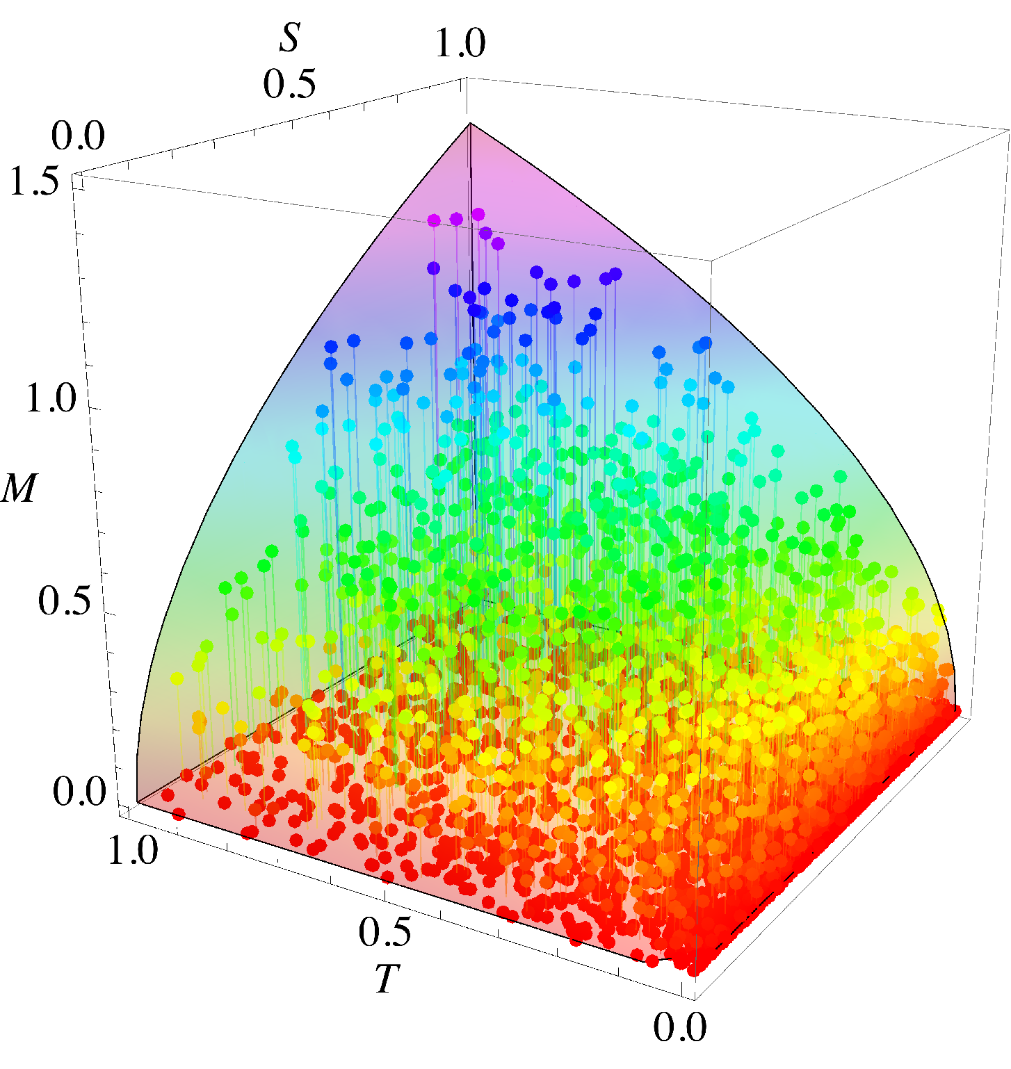
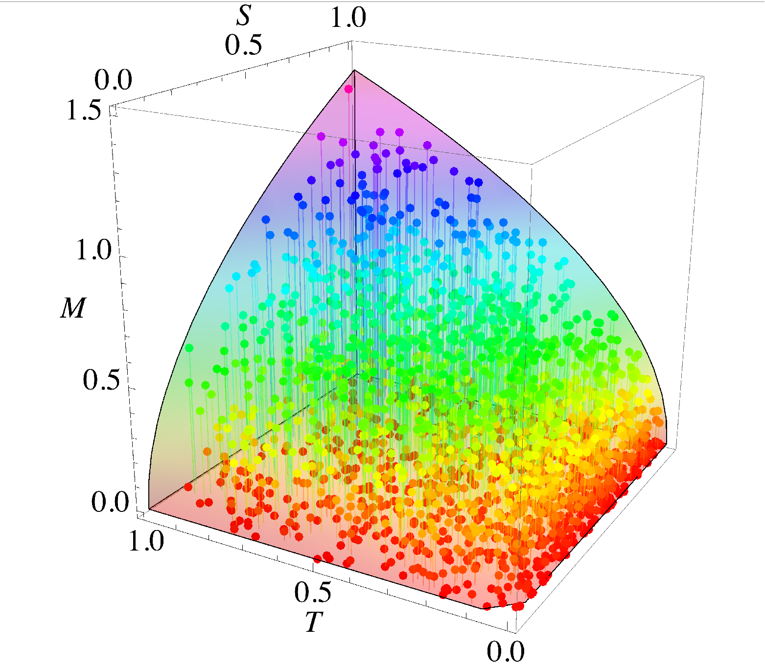
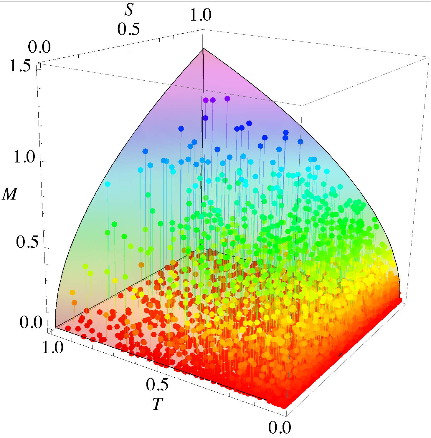
Figure 27: Random points generated in the parameter space of the simplified model, compared with quadratic and quartic positivity bounds in the same space. Top left: quadratic condition from $WW$; Top right: quadratic condition from $ZZ$; Bottom: quadratic condition from $WZ$.

Appendix B Positivity bounds on two operators

Here we list positivity bounds on all two-operator pairs. For $F_{S,i}$ operators:

$$\framebox{$F_{S,0},F_{S,1}$}$$

$$\quad F_{S,0}+F_{S,1}>0\quad(ZZ,L)$$ (333)

$$\quad F_{S,0}>0\quad(WZ,L)$$ (334)

$$\framebox{$F_{S,0},F_{S,2}$}$$

$$\quad F_{S,0}+F_{S,2}>0\quad(ZZ,L;WZ,L)$$ (335)

$$\quad 2F_{S,0}+F_{S,2}>0\quad(WW,L)$$ (336)

$$\framebox{$F_{S,1},F_{S,2}$}$$

$$\quad F_{S,1}+F_{S,2}>0\quad(WW,L;ZZ,L)$$ (337)

$$\quad F_{S,2}>0\quad(WZ,L).$$ (338)

For $F_{T,i}$ operators:

$$\framebox{$F_{T,0},F_{T,1}$}$$

$$\quad 2F_{T,0}+F_{T,1}>0\quad(WW,T_{+-})$$ (339)

$$\quad F_{T,1}>0\quad(WW,T_{++};WZ,T_{\parallel};W\gamma,T_{\parallel})$$ (340)

$$\framebox{$F_{T,0},F_{T,2}$}$$

$$\quad 2F_{T,0}+F_{T,2}>0\quad(WW,T_{+-};ZZ,T_{\parallel};Z\gamma,T_{\parallel})$$ (341)

$$\quad F_{T,2}>0\quad(WW,T_{\perp};WW,T_{++};ZZ,T_{\perp};WZ,T_{\perp};WZ,T_{\parallel};$$

$$\quad\quad W\gamma,T_{\perp};W\gamma,T_{\parallel};Z\gamma,T_{\perp};\gamma\gamma,T_{\perp})$$ (342)

$$\framebox{$F_{T,0},F_{T,5}$}$$

$$\quad 2F_{T,0}-t_{w}^{2}F_{T,5}>0\quad(Z\gamma,T_{\parallel})$$ (343)

$$\quad 2F_{T,0}+F_{T,5}>0\quad(\gamma\gamma,T_{\parallel})$$ (344)

$$\framebox{$F_{T,0},F_{T,6}$}$$

$$\quad F_{T,0}>0\quad(WW,T_{+-};WW,T_{\parallel})$$ (345)

$$\quad F_{T,6}>0\quad(WZ,T_{\parallel})$$ (346)

$$\framebox{$F_{T,0},F_{T,7}$}$$

$$\quad F_{T,7}>0\quad(ZZ,T_{\perp};WZ,T_{\perp};WZ,T_{\parallel};W\gamma,T_{\perp};W\gamma,T_{\parallel};Z\gamma,T_{\perp};\gamma\gamma,T_{\perp})$$ (347)

$$\quad 32c_{w}^{4}F_{T,0}+(8s_{w}^{4}-8s_{w}^{2}+1)F_{T,7}>0\quad(Z\gamma,T_{\parallel})$$ (348)

$$\framebox{$F_{T,0},F_{T,8}$}$$

$$\quad F_{T,0}>0\quad(WW,T_{+-};WW,T_{\parallel})$$ (349)

$$\quad 4T_{T,0}+F_{T,8}>0\quad(\gamma\gamma,T_{\parallel})$$ (350)

$$\framebox{$F_{T,0},F_{T,9}$}$$

$$\quad F_{T,0}>0\quad(WW,T_{+-};WW,T_{\parallel})$$ (351)

$$\quad F_{T,9}>0\quad(ZZ,T_{\perp};Z\gamma,T_{\perp};\gamma\gamma,T_{\perp})$$ (352)

$$\framebox{$F_{T,1},F_{T,2}$}$$

$$\quad F_{T,2}>0\quad(WW,T_{\perp};ZZ,T_{\perp};WZ,T_{\perp};W\gamma,T_{\perp};Z\gamma,T_{\perp};\gamma\gamma,T_{\perp})$$ (353)

$$\quad 4F_{T,1}+F_{T,2}>0\quad(WZ,T_{\parallel};W\gamma,T_{\parallel})$$ (354)

$$\framebox{$F_{T,1},F_{T,5}$}$$

$$\quad 2F_{T,1}-t_{w}^{2}F_{T,5}>0\quad(Z\gamma,T_{\parallel})$$ (355)

$$\quad 2F_{T,1}+F_{T,5}>0\quad(\gamma\gamma,T_{\parallel})$$ (356)

$$\framebox{$F_{T,1},F_{T,6}$}$$

$$\quad F_{T,1}>0\quad(WW,T_{++};WW,T_{+-};WW,T_{\parallel})$$ (357)

$$\quad 2F_{T,1}+F_{T,6}>0\quad(\gamma\gamma,T_{\parallel})$$ (358)

$$\framebox{$F_{T,1},F_{T,7}$}$$

$$\quad F_{T,7}>0\quad(ZZ,T_{\perp};WZ,T_{\perp};W\gamma,T_{\perp};Z\gamma,T_{\perp};\gamma\gamma,T_{\perp})$$ (359)

$$\quad 32c_{w}^{4}F_{T,1}+(8s_{w}^{4}-8s_{w}^{2}+1)F_{T,7}>0\quad(Z\gamma,T_{\parallel})$$ (360)

$$\framebox{$F_{T,1},F_{T,8}$}$$

$$\quad F_{T,1}>0\quad(WW,T_{++};WW,T_{+-};WW,T_{\parallel};WZ,T_{\parallel};W\gamma,T_{\parallel})$$ (361)

$$\quad 4F_{T,1}+F_{T,8}>0\quad(\gamma\gamma,T_{\parallel})$$ (362)

$$\framebox{$F_{T,1},F_{T,9}$}$$

$$\quad F_{T,1}>0\quad(WW,T_{++};WW,T_{+-};WW,T_{\parallel};WZ,T_{\parallel};W\gamma,T_{\parallel})$$ (363)

$$\quad F_{T,9}>0\quad(ZZ,T_{\perp};Z\gamma,T_{\perp};\gamma\gamma,T_{\perp})$$ (364)

$$\framebox{$F_{T,2},F_{T,5}$}$$

$$\quad F_{T,2}-t_{w}^{2}F_{T,5}>0\quad(Z\gamma,T_{\parallel})$$ (365)

$$\quad F_{T,2}+F_{T,5}>0\quad(\gamma\gamma,T_{\parallel})$$ (366)

$$\framebox{$F_{T,2},F_{T,6}$}$$

$$\quad F_{T,2}>0\quad(WW,T_{\perp};WW,T_{++};WW,T_{+-};WW,T_{\parallel};ZZ,T_{\perp};$$

$$\quad\quad\quad\quad WZ,T_{\perp};W\gamma,T_{\perp};Z\gamma,T_{\perp};\gamma\gamma,T_{\perp})$$ (367)

$$\quad F_{T,2}+F_{T,6}>0\quad(\gamma\gamma,T_{\parallel})$$ (368)

$$\framebox{$F_{T,2},F_{T,7}$}$$

$$\quad 16c_{w}^{4}F_{T,2}+(8s_{w}^{4}-8s_{w}^{2}+1)F_{T,7}>0\quad(Z\gamma,T_{\parallel})$$ (369)

$$\quad 2F_{T,2}+F_{T,7}>0\quad(\gamma\gamma,T_{\perp};\gamma\gamma,T_{\parallel})$$ (370)

$$\framebox{$F_{T,2},F_{T,8}$}$$

$$\quad F_{T,2}>0\quad(WW,T_{\perp};WW,T_{++};WW,T_{+-};WW,T_{\parallel};ZZ,T_{\perp};$$

$$\quad\quad\quad\quad WZ,T_{\perp};WZ,T_{\parallel};W\gamma,T_{\perp};W\gamma,T_{\parallel};Z\gamma,T_{\perp};\gamma\gamma,T_{\perp})$$ (371)

$$\quad 2F_{T,2}+F_{T,8}>0\quad(\gamma\gamma,T_{\parallel})$$ (372)

$$\framebox{$F_{T,2},F_{T,9}$}$$

$$\quad F_{T,2}>0\quad(WW,T_{\perp};WW,T_{++};WW,T_{+-};WW,T_{\parallel};$$

$$\quad\quad\quad\quad WZ,T_{\perp};WZ,T_{\parallel};W\gamma,T_{\perp};W\gamma,T_{\parallel})$$ (373)

$$\quad 4F_{T,2}+F_{T,9}>0\quad(\gamma\gamma,T_{\perp};\gamma\gamma,T_{\parallel})$$ (374)

$$\framebox{$F_{T,5},F_{T,6}$}$$

$$\quad-4c_{w}^{2}s_{w}^{2}F_{T,5}+(c_{w}^{2}-s_{w}^{2})^{2}F_{T,6}>0\quad(Z\gamma,T_{\parallel})$$ (375)

$$\quad F_{T,5}+F_{T,6}>0\quad(ZZ,T_{\parallel};\gamma\gamma,T_{\parallel})$$ (376)

$$\framebox{$F_{T,5},F_{T,7}$}$$

$$\quad-16c_{w}^{2}s_{w}^{2}F_{T,5}+(8s_{w}^{4}-8s_{w}^{2}+1)F_{T,7}>0\quad(Z\gamma,T_{\parallel})$$ (377)

$$\quad 2F_{T,5}+F_{T,7}>0\quad(ZZ,T_{\parallel};\gamma\gamma,T_{\parallel})$$ (378)

$$\framebox{$F_{T,5},F_{T,8}$}$$

$$\quad-2F_{T,5}+t_{w}^{2}F_{T,8}>0\quad(Z\gamma,T_{\parallel})$$ (379)

$$\quad 2F_{T,5}+t_{w}^{4}F_{T,8}>0\quad(ZZ,T_{\parallel})$$ (380)

$$\framebox{$F_{T,5},F_{T,9}$}$$

$$\quad-4F_{T,5}+t_{w}^{2}F_{T,9}>0\quad(Z\gamma,T_{\parallel})$$ (381)

$$\quad 4F_{T,5}+t_{w}^{4}F_{T,9}>0\quad(ZZ,T_{\parallel})$$ (382)

$$\framebox{$F_{T,6},F_{T,7}$}$$

$$\quad F_{T,7}>0\quad(ZZ,T_{\perp};WZ,T_{\perp};W\gamma,T_{\perp};Z\gamma,T_{\perp};\gamma\gamma,T_{\perp})$$ (383)

$$\quad 4(c_{w}^{2}-s_{w}^{2})^{2}F_{T,6}+(8s_{w}^{4}-8s_{w}^{2}+1)F_{T,7}>0\quad(Z\gamma,T_{\parallel})$$ (384)

$$\framebox{$F_{T,6},F_{T,8}$}$$

$$\quad F_{T,6}>0\quad(WZ,T_{\parallel};W\gamma,T_{\parallel})$$ (385)

$$\quad 2F_{T,6}+F_{T,8}>0\quad(\gamma\gamma,T_{\parallel})$$ (386)

$$\framebox{$F_{T,6},F_{T,9}$}$$

$$\quad F_{T,9}>0\quad(ZZ,T_{\perp};Z\gamma,T_{\perp};\gamma\gamma,T_{\perp})$$ (387)

$$\quad F_{T,6}>0\quad(WZ,T_{\parallel};W\gamma,T_{\parallel})$$ (388)

$$\framebox{$F_{T,7},F_{T,8}$}$$

$$\quad F_{T,7}>0\quad(ZZ,T_{\perp};WZ,T_{\perp};WZ,T_{\parallel};W\gamma,T_{\perp};W\gamma,T_{\parallel};Z\gamma,T_{\perp};\gamma\gamma,T_{\perp})$$ (389)

$$\quad(8s_{w}^{4}-8s_{w}^{2}+1)F_{T,7}+8s_{w}^{4}F_{T,8}>0\quad(Z\gamma,T_{\parallel})$$ (390)

$$\framebox{$F_{T,7},F_{T,9}$}$$

$$\quad F_{T,7}>0\quad(WZ,T_{\perp};WZ,T_{\parallel};W\gamma,T_{\perp};W\gamma,T_{\parallel})$$ (391)

$$\quad(8s_{w}^{4}-8s_{w}^{2}+1)F_{T,7}+4s_{w}^{4}F_{T,9}>0\quad(Z\gamma,T_{\parallel})$$ (392)

$$\framebox{$F_{T,8},F_{T,9}$}$$

$$\quad F_{T,9}>0\quad(ZZ,T_{\perp};Z\gamma,T_{\perp};\gamma\gamma,T_{\perp})$$ (393)

$$\quad 2F_{T,8}+F_{T,9}>0\quad(ZZ,T_{\parallel};Z\gamma,T_{\parallel};\gamma\gamma,T_{\parallel}).$$ (394)

For $F_{M,i}$ operators,

$$\framebox{$F_{M,0},F_{M,1}$}$$

$$\quad 2F_{M,0}-F_{M,1}>0\quad(ZZ,\overline{M}_{I})$$ (395)

$$\quad-F_{M,0}>0\quad(ZZ,M_{I})$$ (396)

$$\framebox{$F_{M,0},F_{M,7}$}$$

$$\quad-F_{M,0}>0\quad(WW,M_{+-},M_{\parallel};ZZ,M_{I})$$ (397)

$$\quad 4F_{M,0}+F_{M,7}>0\quad(ZZ,\overline{M}_{I})$$ (398)

$$\framebox{$F_{M,1},F_{M,2}$}$$

$$\quad-F_{M,1}+t_{w}^{4}F_{M,2}>0\quad(ZZ,\overline{M}_{I})$$ (399)

$$\quad-F_{M,2}>0\quad(ZZ,M_{I})$$ (400)

$$\framebox{$F_{M,1},F_{M,3}$}$$

$$\quad-F_{M,1}>0\quad(WW,TL,LT;WZ,TL;WW,M_{+-},M_{\parallel};$$

$$\quad\quad\quad\quad WW,\overline{M}_{+-},\overline{M}_{\parallel})$$ (401)

$$\quad-2F_{M,1}-F_{M,3}>0\quad(W\gamma,LT;Z\gamma,LT)$$ (402)

$$\framebox{$F_{M,1},F_{M,4}$}$$

$$\quad-F_{M,1}+t_{w}^{2}F_{M,4}>0\quad(ZZ,\overline{M}_{I})$$ (403)

$$\quad-F_{M,4}>0\quad(ZZ,M_{I})$$ (404)

$$\framebox{$F_{M,1},F_{M,5}$}$$

$$\quad-2F_{M,1}-F_{M,5}>0\quad(Z\gamma,LT)$$ (405)

$$\quad-2F_{M,1}+F_{M,5}>0\quad(W\gamma,LT)$$ (406)

$$\framebox{$F_{M,1},F_{M,7}$}$$

$$\quad-F_{M,1}>0\quad(WW,M_{+-},M_{\parallel})$$ (407)

$$\quad-F_{M,1}+F_{M,7}>0\quad(WZ,\overline{M}^{\prime}_{I})$$ (408)

$$\framebox{$F_{M,2},F_{M,3}$}$$

$$\quad 2F_{M,2}-F_{M,3}>0\quad(ZZ,\overline{M}_{I})$$ (409)

$$\quad-F_{M,2}>0\quad(ZZ,M_{I})$$ (410)

$$\framebox{$F_{M,2},F_{M,7}$}$$

$$\quad 2t_{w}^{4}F_{M,2}+F_{M,7}>0\quad(ZZ,\overline{M}_{I})$$ (411)

$$\quad-F_{M,2}>0\quad(ZZ,M_{I})$$ (412)

$$\framebox{$F_{M,3},F_{M,7}$}$$

$$\quad F_{M,7}>0\quad(WW,TL,LT;WZ,TL;WW,\overline{M}_{+-},\overline{M}_{\parallel})$$ (413)

$$\quad-F_{M,3}>0\quad(WZ,M^{\prime}_{I},\overline{M}^{\prime}_{I})$$ (414)

$$\framebox{$F_{M,4},F_{M,7}$}$$

$$\quad 2t_{w}^{2}F_{M,4}+F_{M,7}>0\quad(ZZ,\overline{M}_{I})$$ (415)

$$\quad-F_{M,4}>0\quad(ZZ,M_{I})$$ (416)

$$\framebox{$F_{M,5},F_{M,7}$}$$

$$\quad F_{M,5}+F_{M,7}>0\quad(W\gamma,LT)$$ (417)

$$\quad-F_{M,5}>0\quad(WZ,M^{\prime}_{I}).$$ (418)

Appendix C Positivity bounds on three operators

Here we list all the three operator bounds considered in Section 6.

$$\framebox{$F_{S,0},F_{S,1},F_{S,2}$}$$

$$\quad F_{S,0}+F_{S,1}+F_{S,2}>0\quad(ZZ,L)$$ (419)

$$\quad 2F_{S,0}+F_{S,1}+F_{S,2}>0\quad(WW,L)$$ (420)

$$\quad F_{S,0}+F_{S,2}>0\quad(WZ,L)$$ (421)

$$\framebox{$F_{T,0},F_{T,1},F_{T,2}$}$$

$$\quad 2F_{T,0}+F_{T,1}+F_{T,2}>0\quad(WW,T_{+-})$$ (422)

$$\quad F_{T,2}>0\quad(WW,T_{\perp};ZZ,T_{\perp};WZ,T_{\perp};W\gamma,T_{\perp};Z\gamma,T_{\perp};\gamma\gamma,T_{\perp})$$ (423)

$$\quad 4F_{T,1}+F_{T,2}>0\quad(WZ,T_{\parallel};W\gamma,T_{\parallel})$$ (424)

$$\quad 2F_{T,0}+2F_{T,1}+F_{T,2}>0\quad(ZZ,T_{\parallel};Z\gamma,T_{\parallel};\gamma\gamma,T_{\parallel})$$ (425)

$$\framebox{$F_{T,5},F_{T,8},F_{T,9}$}$$

$$\quad F_{T,9}>0\quad(ZZ,T_{\perp};Z\gamma,T_{\perp};\gamma\gamma,T_{\perp})$$ (426)

$$\quad-4F_{T,5}+2t_{w}^{2}F_{T,8}+t_{w}^{2}F_{T,9}>0\quad(Z\gamma,T_{\parallel})$$ (427)

$$\quad 4F_{T,5}+2t_{w}^{4}F_{T,8}+t_{w}^{4}F_{T,9}>0\quad(ZZ,T_{\parallel})$$ (428)

$$\framebox{$F_{M,0},F_{M,1},F_{M,2}$}$$

$$\quad 4F_{M,0}-3F_{M,1}>0\quad(WW,\overline{M}_{+-},\overline{M}_{\parallel})$$ (429)

$$\quad-4F_{M,0}-F_{M,1}>0\quad(WW,M_{+-},M_{\parallel})$$ (430)

$$\quad 2F_{M,0}-F_{M,1}+t_{w}^{4}F_{M,2}>0\quad(ZZ,\overline{M}_{I})$$ (431)

$$\quad-2F_{M,0}-t_{w}^{4}F_{M,2}>0\quad(ZZ,M_{I})$$ (432)

$$\framebox{$F_{M,0},F_{M,1},F_{M,3}$}$$

$$\quad-2F_{M,1}-F_{M,3}>0\quad(W\gamma,LT;Z\gamma,LT)$$ (433)

$$\quad 4F_{M,0}-3F_{M,1}>0\quad(WW,\overline{M}_{+-},\overline{M}_{\parallel})$$ (434)

$$\quad 4F_{M,0}-2F_{M,1}-t_{w}^{4}F_{M,3}>0\quad(ZZ,\overline{M}_{I})$$ (435)

$$\quad-F_{M,0}>0\quad(ZZ,M_{I})$$ (436)

$$\framebox{$F_{M,3},F_{M,5},F_{M,7}$}$$

$$\quad F_{M,7}>0\quad(WW,TL,LT;WZ,TL;WW,\overline{M}_{+-},\overline{M}_{\parallel})$$ (437)

$$\quad-F_{M,3}+F_{M,5}+F_{M,7}>0\quad(W\gamma,LT)$$ (438)

$$\quad-t_{w}^{4}F_{M,3}+t_{w}^{2}F_{M,5}+F_{M,7}>0\quad(ZZ,TL,LT;ZZ,\overline{M}_{I})$$ (439)

$$\quad 4F_{M,7}(c_{w}^{4}F_{M,7}-s_{w}^{2}c_{w}^{2}F_{M,5}-s_{w}^{4}F_{M,3})>(2c_{w}^{2}F_{M,7}+s_{w}^{2}F_{M,5})^{2}$$

$$\quad\quad\quad\quad(WZ,M^{\prime}_{I},\overline{M}^{\prime}_{I})$$ (440)

$$\framebox{$F_{M,4},F_{M,5},F_{M,7}$}$$

$$\quad-F_{M,5}+F_{M,7}>0\quad(Z\gamma,LT)$$ (441)

$$\quad F_{M,5}+F_{M,7}>0\quad(W\gamma,LT)$$ (442)

$$\quad 2t_{w}^{2}F_{M,4}+t_{w}^{2}F_{M,5}+F_{M,7}>0\quad(ZZ,\overline{M}_{I})$$ (443)

$$\quad-F_{M,4}>0\quad(ZZ,M_{I})$$ (444)

$$\quad 4F_{M,7}(F_{M,7}-t_{w}^{2}F_{M,5})>(4t_{w}^{2}F_{M,4}+t_{w}^{2}F_{M,5}+2F_{M,7})^{2}$$

$$\quad\quad\quad\quad(WZ,M^{\prime}_{I},\overline{M}^{\prime}_{I})$$ (445)

$$\framebox{$F_{M,1},F_{M,3},F_{M,4}$}$$

$$\quad-2F_{M,1}-F_{M,3}>0\quad(W\gamma,LT;Z\gamma,LT)$$ (446)

$$\quad-F_{M,4}>0\quad(ZZ,M_{I})$$ (447)

$$\quad F_{M,1}(2F_{M,1}+t_{w}^{4}F_{M,3})>2t_{w}^{4}F_{M,4}^{2}\quad(WZ,M^{\prime}_{I},\overline{M}^{\prime}_{I})$$ (448)

$$\framebox{$F_{S,0},F_{T,0},F_{M,7}$}$$

$$\quad F_{S,0}>0\quad(WW,L;ZZ,L;WZ,L)$$ (449)

$$\quad F_{T,0}>0\quad(WW,T_{+-};WW,T_{\parallel};ZZ,T_{\parallel};Z\gamma,T_{\parallel};\gamma\gamma,T_{\parallel})$$ (450)

$$\quad F_{M,7}>0\quad(ZZ,TL,LT;WZ,LT;WW,TL,LT;WZ,TL;$$

$$\quad\quad W\gamma,LT;Z\gamma,LT;WZ,\overline{M}^{\prime}_{I})$$ (451)

$$\framebox{$F_{S,0},F_{T,0},F_{M,0}$}$$

$$\quad F_{S,0}>0\quad(WW,L;ZZ,L;WZ,L)$$ (452)

$$\quad F_{T,0}>0\quad(WW,T_{+-};WW,T_{\parallel};ZZ,T_{\parallel};Z\gamma,T_{\parallel};\gamma\gamma,T_{\parallel})$$ (453)

$$\quad 4F_{S,0}F_{T,0}>F_{M,0}^{2}\quad(ZZ,M_{I},\overline{M}_{I}).$$ (454)

References

- (1) O. J. P. Eboli, M. C. Gonzalez-Garcia and J. K. Mizukoshi, p p j j e+- mu+- nu nu and j j e+- mu-+ nu nu at O( alpha(em)**6) and O(alpha(em)**4 alpha(s)**2) for the study of the quartic electroweak gauge boson vertex at CERN LHC, Phys. Rev. D74 (2006) 073005, [hep-ph/0606118].
- (2) C. Degrande, O. Eboli, B. Feigl, B. Jager, W. Kilian, O. Mattelaer et al., Monte Carlo tools for studies of non-standard electroweak gauge boson interactions in multi-boson processes: A Snowmass White Paper, in Proceedings, 2013 Community Summer Study on the Future of U.S. Particle Physics: Snowmass on the Mississippi (CSS2013): Minneapolis, MN, USA, July 29-August 6, 2013, 2013. 1309.7890.
- (3) O. J. P. Eboli and M. C. Gonzalez-Garcia, Classifying the bosonic quartic couplings, Phys. Rev. D93 (2016) 093013, [1604.03555].
- (4) https://twiki.cern.ch/twiki/bin/view/CMSPublic/PhysicsResultsSMPaTGC#aQGC_Results.
- (5) ATLAS collaboration, Observation of electroweak production of a same-sign boson pair in association with two jets in collisions at TeV with the ATLAS detector, Tech. Rep. ATLAS-CONF-2018-030, CERN, Geneva, Jul, 2018.
- (6) CMS collaboration, A. M. Sirunyan et al., Observation of electroweak production of same-sign W boson pairs in the two jet and two same-sign lepton final state in proton-proton collisions at 13 TeV, Phys. Rev. Lett. 120 (2018) 081801, [1709.05822].
- (7) ATLAS collaboration, Observation of electroweak boson pair production in association with two jets in pp collisions at = 13TeV with the ATLAS Detector, Tech. Rep. ATLAS-CONF-2018-033, CERN, Geneva, Jul, 2018.
- (8) CMS collaboration, Measurement of electroweak WZ production and search for new physics in pp collisions at sqrt(s) = 13 TeV, Tech. Rep. CMS-PAS-SMP-18-001, CERN, Geneva, 2018.
- (9) CMS collaboration, A. M. Sirunyan et al., Measurement of vector boson scattering and constraints on anomalous quartic couplings from events with four leptons and two jets in proton–proton collisions at 13 TeV, Phys. Lett. B774 (2017) 682–705, [1708.02812].
- (10) C. Zhang and S.-Y. Zhou, Positivity bounds on vector boson scattering at the LHC, 1808.00010.
- (11) A. Adams, N. Arkani-Hamed, S. Dubovsky, A. Nicolis and R. Rattazzi, Causality, analyticity and an IR obstruction to UV completion, JHEP 10 (2006) 014, [hep-th/0602178].
- (12) S. Weinberg, Phenomenological Lagrangians, Physica A96 (1979) 327–340.
- (13) W. Buchmuller and D. Wyler, Effective Lagrangian Analysis of New Interactions and Flavor Conservation, Nucl. Phys. B268 (1986) 621–653.
- (14) C. N. Leung, S. T. Love and S. Rao, Low-Energy Manifestations of a New Interaction Scale: Operator Analysis, Z. Phys. C31 (1986) 433.
- (15) J. Elias-Miro, J. R. Espinosa, E. Masso and A. Pomarol, Higgs windows to new physics through d=6 operators: constraints and one-loop anomalous dimensions, JHEP 11 (2013) 066, [1308.1879].
- (16) D. Liu, A. Pomarol, R. Rattazzi and F. Riva, Patterns of Strong Coupling for LHC Searches, JHEP 11 (2016) 141, [1603.03064].
- (17) A. Azatov, R. Contino, C. S. Machado and F. Riva, Helicity selection rules and noninterference for BSM amplitudes, Phys. Rev. D95 (2017) 065014, [1607.05236].
- (18) D. R. Green, P. Meade and M.-A. Pleier, Multiboson interactions at the LHC, Rev. Mod. Phys. 89 (2017) 035008, [1610.07572].
- (19) M. Sekulla, Anomalous couplings, resonances and unitarity in vector boson scattering, Ph.D. thesis (Univ. Siegen, 2015) .
- (20) G. Perez, M. Sekulla and D. Zeppenfeld, Anomalous quartic gauge couplings and unitarization for the vector boson scattering process , Eur. Phys. J. C78 (2018) 759, [1807.02707].
- (21) C. de Rham, S. Melville, A. J. Tolley and S.-Y. Zhou, Positivity bounds for scalar field theories, Phys. Rev. D96 (2017) 081702, [1702.06134].
- (22) C. de Rham, S. Melville, A. J. Tolley and S.-Y. Zhou, UV complete me: Positivity Bounds for Particles with Spin, JHEP 03 (2018) 011, [1706.02712].
- (23) C. de Rham, S. Melville, A. J. Tolley and S.-Y. Zhou, Massive Galileon Positivity Bounds, JHEP 09 (2017) 072, [1702.08577].
- (24) C. de Rham, S. Melville, A. J. Tolley and S.-Y. Zhou, Positivity Bounds for Massive Spin-1 and Spin-2 Fields, 1804.10624.
- (25) B. Bellazzini, Softness and amplitudes’ positivity for spinning particles, JHEP 02 (2017) 034, [1605.06111].
- (26) C. de Rham, S. Melville and A. J. Tolley, Improved Positivity Bounds and Massive Gravity, JHEP 04 (2018) 083, [1710.09611].
- (27) A. Alloul, N. D. Christensen, C. Degrande, C. Duhr and B. Fuks, FeynRules 2.0 - A complete toolbox for tree-level phenomenology, Comput. Phys. Commun. 185 (2014) 2250–2300, [1310.1921].
- (28) T. Hahn, Generating Feynman diagrams and amplitudes with FeynArts 3, Comput. Phys. Commun. 140 (2001) 418–431, [hep-ph/0012260].
- (29) T. Hahn and M. Perez-Victoria, Automatized one loop calculations in four-dimensions and D-dimensions, Comput. Phys. Commun. 118 (1999) 153–165, [hep-ph/9807565].
- (30) B. Grzadkowski, M. Iskrzynski, M. Misiak and J. Rosiek, Dimension-Six Terms in the Standard Model Lagrangian, JHEP 10 (2010) 085, [1008.4884].
- (31) G. Durieux, C. Grojean, J. Gu and K. Wang, The leptonic future of the Higgs, JHEP 09 (2017) 014, [1704.02333].
- (32) CMS collaboration, V. Khachatryan et al., Study of vector boson scattering and search for new physics in events with two same-sign leptons and two jets, Phys. Rev. Lett. 114 (2015) 051801, [1410.6315].
- (33) ATLAS collaboration, G. Aad et al., Evidence for Electroweak Production of in Collisions at TeV with the ATLAS Detector, Phys. Rev. Lett. 113 (2014) 141803, [1405.6241].
- (34) S. Brass, C. Fleper, W. Kilian, J. Reuter and M. Sekulla, Transversal Modes and Higgs Bosons in Electroweak Vector-Boson Scattering at the LHC, Eur. Phys. J. C78 (2018) 931, [1807.02512].
- (35) J. de Blas, J. C. Criado, M. Perez-Victoria and J. Santiago, Effective description of general extensions of the Standard Model: the complete tree-level dictionary, JHEP 03 (2018) 109, [1711.10391].