A generalized lattice Boltzmann model for fluid flow system and its application in two-phase flows

Abstract

In this paper, a generalized lattice Boltzmann (LB) model with a mass source is proposed to solve both incompressible and nearly incompressible Navier-Stokes (N-S) equations. This model can be used to deal with single-phase and two-phase flows problems with a mass source term. From this generalized model, we can not only get some existing models, but also derive new models. Moreover, for the incompressible model derived, a modified pressure scheme is introduced to calculate the pressure, and then to ensure the accuracy of the model. In this work, we will focus on a two-phase flow system, and in the frame work of our generalized LB model, a new phase-field-based LB model is developed for incompressible and quasi-incompressible two-phase flows. A series of numerical simulations of some classic physical problems, including a spinodal decomposition, a static droplet, a layered Poiseuille flow, and a bubble rising flow under buoyancy, are performed to validate the developed model. Besides, some comparisons with previous quasi-incompressible and incompressible LB models are also carried out, and the results show that the present model is accurate in the study of two-phase flows. Finally, we also conduct a comparison between quasi-incompressible and incompressible LB models for two-phase flow problems, and find that in some cases, the proposed quasi-incompressible LB model performs better than incompressible LB models.

1 Introduction

Fluid flow problems are ubiquitous in nature and engineering applications, such as single and multiphase flows [1, 2, 4, 3, 5, 6], thermal flows [7, 8], and porous media flows [9, 5]. For such problems, the phenomenon of fluid flowing in and out of the system is very frequent. In order to describe this phenomenon, an alternative way is to introduce a mass source or sink term in the fluid dynamical equations (i.e., N-S equations) [12, 13, 14, 15]. Besides, in the presence of electro-chemical reactions or multiphase situations, mass sources in the N-S equations could be applied to describe the reaction between the components in the system [12, 16]. Due to limitations of theoretical research and experimental methods, it is especially necessary to develop a numerical method to solve the N-S equations with a mass source term.

As an efficient numerical method, the lattice Boltzmann method has made rapid progress since its appearance in the late 1980s due to its simplicity, scalability on parallel computers, and ease to handle complex geometries [17, 18]. This method has gained great success in the study of fluid flow system [19, 20, 21, 22]. In general, LB methods for dealing with such flow problems can be divided into two categories. One is the nearly incompressible model and the other is the so-called incompressible model. For the nearly incompressible model, the macroscopic quantities those need to be solved are the density $\rho$ and fluid velocity $\mathbf{u}$, and the pressure can be obtained from the equation of state ($p=\rho c_{s}^{2}$). While for the incompressible model, the macroscopic quantities we need to calculate are fluid velocity $\mathbf{u}$ and the pressure $p$, where density $\rho$ is viewed as a constant. In the past, people always considered these two types of models separately. Actually, from the perspective of model construction, one can design a generalized LB model to deal with both incompressible and nearly incompressible problems, which is the main motivation of this paper. Moreover, some previous models have more or less assumptions in the derivation process, and often cannot recover the macroscopic equations completely. In addition, under the framework of LB methods, people have less research on N-S equations with a mass source term. For instance, Halliday et al. [23] proposed a single-relaxation-time (SRT) LB model including a mass source term, while they employed a non-local scheme to calculate the spatial derivatives which appear in the source term. Cheng et al. [24] presented another LB model with a general mass source term and adopted a non-local scheme for temporal and spatial derivatives. Aursjø et al. [12] also developed an SRT model with a mass source term, which does not include temporal and spatial derivatives in the source term, and it preserves the Galilean invariance. We note that the above models are limited to nearly incompressible situations. While, up to now, there is no available work on incompressible N-S equations with a mass source term. Considering the above points, in this work, we will develop a generalized SRT LB model for both incompressible and nearly incompressible N-S equations with a mass source term, and this model is also an extension of existing models. From the generalized model, we can not only get some existing models, but also derive new models. Among these new models, we can obtain an incompressible model for N-S equations with a mass source term, and we present a modified scheme to calculate the pressure $p$, which is more accurate than the previous one. Simultaneously, our generalized model can recover the macroscopic equations without any unnecessary assumptions. Finally, we would like to point that this model can be used not only to solve single-phase fluid flows, but also to design models for two-phase flows.

Based on our generalized model, we also present a phase-field-based LB model for two-phase flows. The present model contains both quasi-incompressible and incompressible situations, in which the quasi-incompressible model can guarantee the mass conservation, and its governing equation of the flow field can be regarded as a kind of incompressible N-S equation with a mass source term. Actually, there are also some phase-field-based LB models for incompressible two-phase flows. He et al. [2] proposed a phase-field LB model and adopted an order parameter to track the interface of two incompressible fluids. However, there are some differences between the derived governing equations and the phase-field theory for incompressible two-phase flows [25]. To recover the Cahn-Hilliard (CH) equation correctly, Zheng et al. [26] and Zu et al. [25] developed two different LB models, while, the extra terms in the recovered macroscopic equations from their models will produce large errors in the interface capturing, and numerical instability will occur when the dimensionless relaxation time equals to $1$ [25]. To overcome these problems, Liang et al. [27] proposed a new multi-relaxation-time (MRT) LB model through introducing a time-dependent source term in the evolution equation of phase field. While all the above models cannot conserve mass locally when the densities of the two fluids are different. To solve the problem, Yang et al. [10] presented a modified LB model based on the quasi-incompressible theory. From his model, the quasi-incompressible N-S equations in artificial compressible form can be derived. To neglect the artificial compressible effect, the model requires an additional condition, $T\gg L/c_{s}$ ($T$ and $L$ are characteristic time and length, respectively). Based on the work of Yang et al. [10], Zhang et al. [28] proposed a discrete unified gas-kinetic scheme (DUGKS) for two-phase flows which can exactly guarantee the mass conservation, while this model also give rise to the generation of artificial compressible effect. On the contrary, the present phase-field-based LB model can overcome the above defects. The rest of present paper is organized as follows. In Sec. II, the generalized LB model for fluid flow system with a mass source is introduced, and a phase-field-based LB model for two-phase flows is given in Sec. III. Numerical experiments to validate the present model are carried out in Sec. IV. Finally, some conclusions are given in Sec. V.

2 Generalized LB model for fluid flow system with a mass source

2.1 Governing equations

The governing equations for nearly incompressible fluid flows with a mass source term can be written as [12, 30, 31]

$$\frac{\partial{\rho}}{\partial t}+\nabla\cdot\left(\rho\textbf{u}\right)=S,$$ (1a)

$$\begin{split}\frac{\partial(\rho\textbf{u})}{\partial t}+\nabla\cdot\left(\rho\textbf{u}\textbf{u}\right)=&-\nabla\emph{p}+\nabla\cdot\tau+\textbf{F},\end{split}$$ (1b)

where $\rho$ is the density, u denotes the fluid velocity, $S$ is a mass source or sink term, p is the hydrodynamic pressure, F is the external force, $\tau$ is the deviatoric stress tensor, and for Newtonian fluids,

$$\begin{split}\tau=&\mu(\nabla\textbf{u}+\nabla\textbf{u}^{\emph{T}})+\left(\xi-\frac{2}{d}\mu\right)\nabla\cdot\mathbf{u}\mathbf{I}\end{split}$$ (2)

where $\mu$ denotes the dynamic viscosity by $\mu=\rho\nu$, $\nu$ is the kinematic viscosity, $\xi$ is the bulk (or volume) viscosity and $d$ is the number of spatial dimensions.

If we take $S=0$ in Eq. (1b), the governing equations for nearly incompressible fluid flow system can be obtained [17],

$$\frac{\partial{\rho}}{\partial t}+\nabla\cdot\left(\rho\textbf{u}\right)=0,$$ (3a)

$$\begin{split}\frac{\partial(\rho\textbf{u})}{\partial t}+\nabla\cdot\left(\rho\textbf{u}\textbf{u}\right)=&-\nabla\emph{p}+\nabla\cdot\tau+\textbf{F},\end{split}$$ (3b)

For fluid flows with small temperature changes, the flow can be regarded as incompressible under the condition of $\rho=const$, so that the above governing equations will reduce to [17, 20]

$$\nabla\cdot\textbf{u}=0,$$ (4a)

$$\begin{split}\frac{\partial\textbf{u}}{\partial t}+\nabla\cdot\left(\textbf{u}\textbf{u}\right)=&-\nabla\emph{p}+\nabla\cdot[\nu(\nabla\mathbf{u})]+\mathbf{F}.\end{split}$$ (4b)

In this work, to simplify the following discussion and facilitate the design of a generalized model, here we consider the following generalized governing equations with a mass source,

$$\frac{\partial\tilde{\rho}}{\partial t}+\nabla\cdot\left({\rho}\textbf{u}\right)=S,$$ (5a)

$$\begin{split}\frac{\partial({\rho}\textbf{u})}{\partial t}+\nabla\cdot\left({\rho}\textbf{u}\textbf{u}\right)=&-\nabla\emph{p}+\nabla\cdot\tau+\textbf{F},\end{split}$$ (5b)

where $\tilde{\rho}$ is physical quantity related to $\rho$ or a constant. Note that Eqs. (5b) are a kind of generalized N-S equations which contain two basic forms of incompressible and nearly incompressible governing equations, and they can be used to describe single-phase or multi-phase flows with a mass source term. When $\tilde{\rho}$ and $S$ take different values, Eqs. (5b) represents different governing equations. For example, if we take $\tilde{\rho}=\rho$, Eqs. (5b) will reduce to Eqs. (1b), and further reduce to Eqs. (3b) with $S=0$. While if we take $\tilde{\rho}=\rho=const$, and $S=0$, Eqs. (4b) can be derived. Next, we will design the corresponding LB model for Eqs (5b), and the designed model must be able to deal with the incompressible and near incompressible single-phase and multi-phase flow problems with a mass source term. From this perspective, the LB model we designed is also a generalized model.

2.2 LB model for generalized N-S equations with a mass source term

To obtain the evolution equation of Eq. (5b), we integrate the following discrete velocity Boltzmann equation

$$\frac{\partial f_{i}}{\partial t}+\mathbf{c}_{i}\cdot\nabla f_{i}=\Omega_{i}+G_{i}$$ (6)

along a characteristic line $\mathbf{c}_{i}$ over a time interval $\Delta t$ [33, 34], and we have

$$f_{i}(\textbf{x}+\textbf{c}_{i}\Delta t,t+\Delta t)-f_{i}(\textbf{x},t)=\int_{0}^{\Delta t}\Omega_{i}(\textbf{x}+\textbf{c}_{i}t^{\prime},t+t^{\prime})dt^{\prime}+\int_{0}^{\Delta t}G_{i}(\textbf{x}+\textbf{c}_{i}t^{\prime},t+t^{\prime})dt^{\prime}.$$ (7)

where $f_{i}(\mathbf{x},t)$ denotes particle distribution function with velocity $\mathbf{c}_{i}$ at position $\mathbf{x}$ and time $t$, $G_{i}(\mathbf{x},t)$ represents the force term, $\Omega_{i}(\mathbf{x},t)$ is the collision operator approximated by

$$\Omega_{i}=-\frac{1}{\tau^{\prime}}(f_{i}-f_{i}^{eq}),$$ (8)

where $\tau^{\prime}$ is the relaxation time and $f_{i}^{eq}(\mathbf{x},t)$ is the equilibrium distribution function.

The integral of the collision term adopts the trapezoidal rule, then Eq. (7) becomes

$$f_{i}(\textbf{x}+\textbf{c}_{i}\Delta t,t+\Delta t)-f_{i}(\textbf{x},t)=\frac{\Delta t}{2}\left[\Omega_{i}(\textbf{x}+\textbf{c}_{i}\Delta t,t+\Delta t)+\Omega_{i}(\textbf{x},t)\right]+\int_{0}^{\Delta t}G_{i}(\textbf{x}+\textbf{c}_{i}t^{\prime},t+t^{\prime})dt^{\prime}.$$ (9)

Let $\bar{f}_{i}=f_{i}-\frac{\Delta t}{2}\Omega_{i}$, we have

$$\bar{f}_{i}(\textbf{x}+\textbf{c}_{i}\Delta t,t+\Delta t)-\bar{f}_{i}(\textbf{x},t)=-\frac{1}{\tau_{g}}\left[\bar{f}_{i}(\mathbf{x},t)-f_{i}^{eq}(\mathbf{x},t)\right]+\int_{0}^{\Delta t}G_{i}(\textbf{x}+\textbf{c}_{i}t^{\prime},t+t^{\prime})dt^{\prime},$$ (10)

where $\tau_{g}=\frac{2\tau^{\prime}+\Delta t}{2\Delta t}$ is the dimensionless relaxation time, and $\bar{f}_{i}$ satisfies $\sum_{i}\bar{f}_{i}=\sum_{i}f_{i}$, and $\sum_{i}\mathbf{c}_{i}\bar{f}_{i}=\sum_{i}\mathbf{c}_{i}f_{i}$.

Through Taylor expansion of $G_{i}$ and neglecting the terms of order $O(\Delta t^{2})$, the last term in the right hand of Eq. (10) becomes

$$\begin{split}\int_{0}^{\Delta t}G_{i}(\textbf{x}+\textbf{c}_{i}\Delta t^{\prime},t+\Delta t^{\prime})dt^{\prime}&=\int_{0}^{\Delta t}\left(G_{i}(\mathbf{x},t)+t^{\prime}D_{i}G_{i}(\mathbf{x},t)\right)dt^{\prime}\\ &=\Delta tG_{i}(\mathbf{x},t)+\frac{\Delta t^{2}}{2}D_{i}G_{i}(\mathbf{x},t),\end{split}$$ (11)

where $D_{i}=\partial t+\mathbf{c}_{i}\cdot\nabla$.

The LB evolution equation with the BGK collision operator for the N-S equations can be expressed as [34]

$$\bar{f}_{i}(\textbf{x}+\textbf{c}_{i}\Delta t,t+\Delta t)-\bar{f}_{i}(\textbf{x},t)=-\frac{1}{\tau_{g}}\left[\bar{f}_{i}(\mathbf{x},t)-f_{i}^{eq}(\mathbf{x},t)\right]+\Delta t\left[G_{i}(\mathbf{x},t)+\frac{\Delta t}{2}D_{i}G_{i}\right],$$ (12)

If the up-wind scheme is used to Eq. (12), the evolution equation for the generalized N-S equations reads

$$\bar{f}_{i}(\textbf{x}+\textbf{c}_{i}\Delta t,t+\Delta t)-\bar{f}_{i}(\textbf{x},t)=-\frac{1}{\tau_{g}}\left[\bar{f}_{i}(\mathbf{x},t)-f_{i}^{eq}(\mathbf{x},t)\right]+\Delta t\left[G_{i}(\mathbf{x},t)+\frac{G_{i}(\textbf{x}+\textbf{c}_{i}\Delta t,t+\Delta t)-G_{i}(\textbf{x},t)}{2}\right].$$ (13)

To remove the implicitness, we introduce a modified particle distribution function,

$$g_{i}(\mathbf{x},t)=\bar{f}_{i}(\mathbf{x},t)-\frac{\Delta t}{2}G_{i}.$$ (14)

With some simple manipulations, the explicit evolution equation can be derived,

$$g_{i}(\textbf{x}+\textbf{c}_{i}\Delta t,t+\Delta t)-g_{i}(\textbf{x},t)=-\frac{1}{\tau_{g}}\left(g_{i}(\mathbf{x},t)-g_{i}^{eq}(\mathbf{x},t)\right)+\Delta t(1-\frac{1}{2\tau_{g}})G_{i},$$ (15)

where $g_{i}^{eq}$ is the new equilibrium distribution function and satisfies $g_{i}^{eq}=f_{i}^{eq}$.

To derive Eq. (5b) through Chapman-Enskog analysis, the equilibrium distribution function $g_{i}^{eq}$ is defined as (see A for the details)

$$g_{i}^{eq}=\left\{\begin{array}[]{l}\tilde{\rho}+\frac{p}{c_{s}^{2}}(\omega_{i}-1)+{\rho}s_{i}(\mathbf{u}),\;\;\;i=0\\ \frac{p}{c_{s}^{2}}\omega_{i}+{\rho}s_{i}(\mathbf{u}),\;\;\;\;\;\;\;\;\;\;\;\;\;\;\;\;\;i\neq 0,\end{array}\right.$$ (16)

with

$$s_{i}({\mathbf{u}})=\omega_{i}\left[\frac{\mathbf{c}_{i}\cdot\mathbf{u}}{c_{s}^{2}}+\frac{(\mathbf{c}_{i}\cdot\mathbf{u})^{2}}{2c_{s}^{4}}-\frac{\mathbf{u}\cdot\mathbf{u}}{2c_{s}^{2}}\right],$$ (17)

where $\omega_{i}$ denotes the weighting coefficient, $\mathbf{c}_{i}$ is the discrete velocity, and $c_{s}$ is the speed of sound. Note that our model is based on the D$d$Q$q$ lattice with $q$ velocity directions in $d$-dimensional space. $\mathbf{c}_{i}$ and $\omega_{i}$ depend on the choice of the lattice model, and in D$1$Q$3$ model, $\{\mathbf{c}_{i}\}=(0,1,-1)c$, $\omega_{0}=2/3$, $\omega_{1,2}=1/6$, $c_{s}=c/\sqrt{3}$, where $c=\Delta x/\Delta t$ , with $\Delta x$ and $\Delta t$ representing the spacing and time step, respectively; while in the D$2$Q$9$ model, $\omega_{i}$ is given by $\omega_{0}=4/9$, $\omega_{1-4}=1/9$, $\omega_{5-8}=1/36$, $c_{s}=c/\sqrt{3}$, and $\mathbf{c}_{i}$ is given by

$$\{\mathbf{c}_{i}\}=\left(\begin{array}[]{rrrrrrrrr}0&1&0&-1&0&1&-1&-1&1\\ 0&0&1&0&-1&1&1&-1&-1\end{array}\right)c;$$

in the D$3$Q$15$ model, $\omega_{0}=2/9$, $\omega_{1-6}=1/9$, $\omega_{7-14}=1/72$, $c_{s}=c/\sqrt{3}$, and $\mathbf{c}_{i}$ is given by

$$\{\mathbf{c}_{i}\}=\left(\begin{array}[]{rrrrrrrrrrrrrrr}0&1&0&0&-1&0&0&1&1&1&-1&-1&-1&-1&1\\ 0&0&1&0&0&-1&0&1&1&-1&1&-1&-1&1&-1\\ 0&0&0&1&0&0&-1&1&-1&1&1&-1&1&-1&-1\end{array}\right)c.$$

Different from some previous LB models [39, 10, 27, 36, 37, 25, 35, 38], in the present model, the force distribution function is given by

$$G_{i}=\omega_{i}\left\{S+\frac{\mathbf{c}_{i}\cdot\mathbf{F}}{c_{s}^{2}}+\frac{(\mathbf{c}_{i}\mathbf{c}_{i}-c_{s}^{2}\mathbf{I}):\left[\partial_{t}(p-\tilde{\rho}c_{s}^{2})\mathbf{I}+\mathbf{u\tilde{F}}+\mathbf{\tilde{F}u}-\mathbf{uu}\tilde{S}+Q(\nabla\cdot\mathbf{uI})\right]}{2c_{s}^{4}}\right\},$$ (18)

where $\tilde{\mathbf{F}}$ is a modified total force

$$\mathbf{\tilde{F}}=\mathbf{F}-\nabla(p-{\rho}c_{s}^{2}),$$ (19)

$\tilde{S}$ and $Q$ can be expressed as

$$\tilde{S}=S+\partial_{t}({\rho}-\tilde{\rho}).$$ (20)

$$Q=\frac{2}{d}{\rho}c_{s}^{2}-\frac{\xi}{\Delta t(\tau_{g}-0.5)}.$$ (21)

Under the Stokes hypothesis, the bulk viscosity $\xi$ is usually assumed to be zero [32]. In addition, $\xi$ can also take $2\rho\nu/d$, so that the derived macroscopic equations will not contain the term $\left(\xi-\frac{2}{d}\mu\right)\nabla\cdot\mathbf{u}\mathbf{I}$. Please note that $G_{i}$ is a complete form and doesn’t contain any unnecessary assumptions, and $G_{i}$ can be reasonably simplified for specific problems.

We would like to point out that through the Chapman-Enskog analysis, the present LB model with the force term Eq. (18) can correctly recover Eq. (5b) (see A for the details), and simultaneously, the fluid kinematic viscosity can be determined by

$$\nu=c_{s}^{2}(\tau_{g}-0.5)\Delta t.$$ (22)

In the implementation of the present model, for nearly incompressible model, the macroscopic quantities $\tilde{\rho}$ can be calculated as

$$\tilde{\rho}=\sum_{i}g_{i}+\frac{\Delta t}{2}S,$$ (23)

where Eq. (14) is used. By taking the first-order moment of $g_{i}$, the fluid velocity can be obtained [27, 6, 31],

$$\mathbf{u}=\frac{1}{{\rho}}\left(\sum_{i}\mathbf{c}_{i}g_{i}+0.5\Delta t\mathbf{F}\right).$$ (24)

While for the incompressible model, the macroscopic quantities we need to calculate are fluid velocity $\mathbf{u}$ and the pressure $p$. The fluid velocity is given by Eq. (24), and the pressure can be calculated as (see B for the details)

$$p=\frac{c_{s}^{2}}{1-\omega_{0}}\left[\sum_{i\neq 0}g_{i}+\frac{\Delta t}{2}S+{\rho}s_{0}(\mathbf{u})+\Delta t(\tau_{g}-\frac{1}{2})G_{0}\right],$$ (25)

or

$$p=\frac{c_{s}^{2}}{1-\omega_{0}}\left[\sum_{i\neq 0}g_{i}+\frac{\Delta t}{2}S+{\rho}s_{0}(\mathbf{u})+\Delta t(\tau_{g}-\frac{1}{2})(S-\sum_{i\neq 0}G_{i})\right].$$ (26)

We would also like to point out that the present pressure expression is different from that in Refs. [27, 31, 35] which can be expressed as

$$p=\frac{c_{s}^{2}}{1-\omega_{0}}\left[\sum_{i\neq 0}g_{i}+\frac{\Delta t}{2}S+\rho s_{0}(\mathbf{u})\right],$$ (27)

where the term of $\Delta t(\tau_{g}-\frac{1}{2})G_{0}$ has been neglected. However, the last term $\Delta t(\tau-\frac{1}{2})G_{0}$ may be significant since $G_{0}$ is usually nonzero under the condition of $S\neq 0$, and the effect of this item cannot be ignored.

Thus, our generalized LB model for fluid flow system are made up of Eqs. (15), (16), (18) and (23), (24) or (24), (25). In the derivation of the model, we only used the assumption of low Mach number ($Ma\ll 1$), which is necessary for the construction of most LB models. Under this assumption, the following equations are established for nearly incompressible or incompressible flows, $\mathbf{u}=O(Ma)$, $\delta\rho=O(Ma^{2})$, and $\delta p=O(Ma^{2})$. Further, we have $\mathbf{F}=O(Ma)$ and $S=O(Ma)$. Now, we will use some remarks to show that our model not only contains some existing models, but also deduces new models for N-S equations with a mass source term.

Remark 1. When taking $\tilde{\rho}=\rho$ and $p=\rho c_{s}^{2}$, the generalized model can reduce to the nearly incompressible form. Correspondingly, the macroscopic equations becomes Eqs. (1b), while the equilibrium distribution function can be written as

$$g_{i}^{eq}=\rho\left[\omega_{i}+s_{i}(\mathbf{u})\right],$$ (28)

and the force distribution function is given by

$$G_{i}=\omega_{i}\left\{S+\frac{\mathbf{c}_{i}\cdot\mathbf{F}}{c_{s}^{2}}+\frac{(\mathbf{c}_{i}\mathbf{c}_{i}-c_{s}^{2}\mathbf{I}):\left[\mathbf{u{F}}+\mathbf{{F}u}-\mathbf{uu}{S}+Q(\nabla\cdot\mathbf{uI})\right]}{2c_{s}^{4}}\right\},$$ (29)

where the term $\mathbf{uu}{S}$ is the order of $O(Ma^{3})$ and can be neglected. This model is almost identical to the one in Ref. [12], except that the expression of the momentum equation and the value of bulk viscosity are different.

Remark 2. If we rewrite the equilibrium distribution function Eq. (28) to the following form,

$$g_{i}^{eq}=\omega_{i}\left\{\rho+(\rho_{0}+\delta\rho)\left[\frac{\mathbf{c}_{i}\cdot\mathbf{u}}{c_{s}^{2}}+\frac{(\mathbf{c}_{i}\cdot\mathbf{u})^{2}}{2c_{s}^{4}}-\frac{\mathbf{u}\cdot\mathbf{u}}{2c_{s}^{2}}\right]\right\}.$$ (30)

Multiplying by $c_{s}^{2}$ on both sides of Eq. (30) and ignoring the term of $O(Ma^{2})$, one can get

$$g_{i}^{eq}=\omega_{i}\left\{p+p_{0}\left[\frac{\mathbf{c}_{i}\cdot\mathbf{u}}{c_{s}^{2}}+\frac{(\mathbf{c}_{i}\cdot\mathbf{u})^{2}}{2c_{s}^{4}}-\frac{\mathbf{u}\cdot\mathbf{u}}{2c_{s}^{2}}\right]\right\},$$ (31)

where we still use $g_{i}^{eq}$ to represent the new equilibrium distribution function. The force distribution function is given by

$$G_{i}=\omega_{i}\left\{p_{0}S_{1}+\frac{p_{0}\mathbf{c}_{i}\cdot\mathbf{F_{1}}}{c_{s}^{2}}+\frac{(\mathbf{c}_{i}\mathbf{c}_{i}-c_{s}^{2}\mathbf{I}):\left[p_{0}(\mathbf{u{F_{1}}}+\mathbf{{F_{1}}u})+\left(\frac{2}{d}{p_{0}}c_{s}^{2}-\frac{\xi}{\Delta t(\tau_{g}-0.5)}\right)(\nabla\cdot\mathbf{uI})\right]}{2c_{s}^{4}}\right\},$$ (32)

where $p_{0}=const$, $S_{1}=\frac{S}{p_{0}}$, $F_{1}=\frac{F}{p_{0}}$, and the terms of $O(Ma^{3})$ are abandoned in the incompressible limit. The fluid velocity and pressure can be obtained by $p=\sum_{i}g_{i}+\frac{\Delta t}{2}p_{0}S_{1}$ and $p_{0}\mathbf{u}=\sum_{i}c_{i}g_{i}+\frac{\Delta t}{2}p_{0}\mathbf{F_{1}}$. The corresponding incompressible N-S equations with a source term $S_{1}$ can be obtained from Eqs. (5b),

$$\frac{1}{c_{s}^{2}}\frac{\partial P}{\partial t}+\nabla\cdot\textbf{u}=S_{1},$$ (33a)

$$\begin{split}\frac{\partial\textbf{u}}{\partial t}+\nabla\cdot\left(\textbf{u}\textbf{u}\right)=&-\nabla{P}+\nabla\cdot[\nu(\nabla\mathbf{u}+\nabla\mathbf{u}^{\emph{T}})]+\nabla\cdot[(-\frac{2}{3}\nu)\nabla\cdot\mathbf{uI}]+\textbf{F}_{1},\end{split}$$ (33b)

where $P=\frac{p}{\rho_{0}}$. In the limit of a low Mach number ($Ma=|\mathbf{u}|/c_{s}^{2}$), the dynamic pressure is assumed to be $\delta p\sim Ma^{2}$ and the left end term of Eq. (33a) can be ignored. Note that if we take $S_{1}=0$, this model can reduce to the incompressible LB model by He et al. [19].

Remark 3. When taking $\tilde{\rho}=\rho_{0}$, ${\rho}=const$ (e.g., ${\rho}=1$), where $\rho_{0}$ is the average velocity of the fluid, we can derive a new model for incompressible N-S equations with a mass source term. In this case, the macroscopic equations can be written as [see Eqs. (5b)]

$$\nabla\cdot\textbf{u}=S,$$ (34a)

$$\begin{split}\frac{\partial\textbf{u}}{\partial t}+\nabla\cdot\left(\textbf{u}\textbf{u}\right)=&-\nabla\emph{p}+\nabla\cdot[\nu(\nabla\mathbf{u}+\nabla\mathbf{u}^{\emph{T}})]+\nabla\cdot[(-\frac{2}{3}\nu)\nabla\cdot\mathbf{uI}]+\textbf{F}.\end{split}$$ (34b)

The corresponding equilibrium distribution function can be derived from Eq. (16)

$$g_{i}^{eq}=\left\{\begin{array}[]{l}\rho_{0}+\frac{p}{c_{s}^{2}}(\omega_{i}-1)+s_{i}(\mathbf{u}),\;\;\;i=0\\ \frac{p}{c_{s}^{2}}\omega_{i}+s_{i}(\mathbf{u}),\;\;\;\;\;\;\;\;\;\;\;\;\;\;\;\;\;\;i\neq 0,\end{array}\right.$$ (35)

and the force distribution function is given by

$$G_{i}=\omega_{i}\left\{S+\frac{\mathbf{c}_{i}\cdot\mathbf{F}}{c_{s}^{2}}+\frac{(\mathbf{c}_{i}\mathbf{c}_{i}-c_{s}^{2}\mathbf{I}):\left[\mathbf{u{F}}+\mathbf{{F}u}+QS\mathbf{I}\right]}{2c_{s}^{4}}\right\},$$ (36)

where the term $\mathbf{uu}{\tilde{S}}$ and $\partial_{t}p$ are neglect in the incompressible limit.

We note that if we take $S=0$, this model can reduce to the incompressible LB model by Guo et al. [20] with a force term, i.e., Eqs. (4b).

Remark 4. Eq. (24) may be implicit if the force $\mathbf{F}$ is a nonlinear function of $\mathbf{u}$. To remove this implicitness, we can discretize $D_{i}G_{i}$ by [34]

$$D_{i}G_{i}=\frac{G_{i}(\textbf{x}+\textbf{c}_{i}\Delta t,t)-G_{i}(\textbf{x},t-\Delta t)}{\Delta t}.$$ (37)

Then the evolution equation can be rewritten as

$$g_{i}(\textbf{x}+\textbf{c}_{i}\Delta t,t+\Delta t)-g_{i}(\textbf{x},t)=-\frac{1}{\tau_{g}}\left(g_{i}(\mathbf{x},t)-g_{i}^{eq}(\mathbf{x},t)\right)+\Delta t\left[G_{i}(\mathbf{x},t)+\frac{G_{i}(\textbf{x}+\textbf{c}_{i}\Delta t,t)-G_{i}(\textbf{x},t-\Delta t)}{2}\right].$$ (38)

This scheme is explicit and can be iterated if $G_{i}$ is known, while the results of $G_{i}$ at time $t-\Delta t$ must be saved additionally.

3 Phase-field-based LB model for two-phase flows

In Sec. II, we have given the generalized LB model for single-phase flows with a mass source term. Actually, one of the motivations of the generalized model is to deal with the two-phase flow problems based on phase-field theory.

3.1 Governing equations

In the classic theory of phase field model for two-phase flows, the N-S equations are employed to describe the flow field, while the Cahn-Hilliard (C-H) equation is usually adopted to capture the phase interface which can be given by [29, 40, 41]

$$\frac{\partial\phi}{\partial t}+\nabla\cdot\phi\textbf{u}=\nabla\cdot M_{\phi}\left(\nabla\mu\right),$$ (39)

where $M_{\phi}$ is the mobility coefficient, $\phi$ is the order parameter defined as the volume fraction of one of the two phases, and $\phi$ and $\rho$ satisfy the linear relationship,

$$\frac{\rho-\rho_{B}}{\rho_{A}-\rho_{B}}=\frac{\phi-\phi_{B}}{\phi_{A}-\phi_{B}}.$$ (40)

In this work, $\phi=0$ denotes the phase B while $\phi=1$ represents the phase A, and $\mu$ is the chemical potential, which is derived by the variation of the free-energy function $F(\phi)$ with respect to the order parameter [29, 42, 43],

$$\begin{split}\mu&=\frac{\delta F(\phi)}{\delta\phi}=\frac{d\psi(\phi)}{d\phi}-\kappa\nabla^{2}\phi\\ &=4\beta\phi(\phi-1)(\phi-0.5)-\kappa\nabla^{2}\phi.\end{split}$$ (41)

where $F(\phi)$ can be taken as the following form [29, 40, 41, 44],

$$F(\phi)=\int_{\Omega}\left[\psi\left(\phi\right)+\frac{\kappa}{2}\left|\nabla\phi\right|^{2}\right]\,d\Omega,$$ (42)

where $\Omega$ is the physical domain of the system, $\psi\left(\phi\right)$ denotes the bulk free-energy density, and $k\left|\nabla\phi\right|^{2}/2$ accounts for the surface energy with a positive coefficient $k$. If the system considered is a van der Waals fluid, the bulk free energy has a double-well form [29],

$$\psi(\phi)=\beta\phi^{2}(\phi-1)^{2},$$ (43)

where $\beta$ is a constant dependent on the interfacial thickness $W$ and the surface tension $\sigma$ [29],

$$W=\sqrt{\frac{8\kappa}{\beta}}$$ (44)

and

$$\sigma=\frac{\sqrt{2\kappa\beta}}{6}.$$ (45)

The equilibrium interface profile can be obtained by minimizing $F(\phi)$ with respect to the function $\phi$ , i.e., $\mu=0$ . In a plane interface at the equilibrium condition, the order parameter profile across the interface (along the $z$ direction) is represented by [43]

$$\phi(z)=\frac{1}{2}+\frac{1}{2}\tanh\left(\frac{2z}{W}\right).$$ (46)

In the present work, we will focus on the following quasi-incompressible phase-field system, and the governing equations are described as

$$\frac{\partial\phi}{\partial t}+\nabla\cdot\phi\textbf{u}=\nabla\cdot M_{\phi}\left(\nabla\mu\right),$$ (47a)

$$\nabla\cdot\textbf{u}=S_{1},$$ (47b)

$$\begin{split}\frac{\partial(\rho\textbf{u})}{\partial t}+\nabla\cdot\left(\rho\textbf{u}\textbf{u}\right)=&-\nabla\emph{p}+\nabla\cdot\tau+\textbf{F},\end{split}$$ (47c)

where $\mathbf{F}$ represents the total force which is defined as $\mathbf{F}_{s}+\mathbf{G}$, and $\mathbf{G}$ is the body force, $\mathbf{F}_{s}$ is the surface tension with the potential form $\mathbf{F}_{s}=\mu\nabla\phi$ [29, 45] if not specified. Eq. (47b) can be derived from Eq. (5a), if $S=\mathbf{u}\cdot\nabla\rho+\rho S_{1}$, and $\tilde{\rho}=\rho_{0}$.

3.2 The LB model for quasi-incompressible phase-field system

3.2.1 LB model for the N-S equations

Based on the generalized LB model for fluid flow system, one can get the equilibrium and force distribution function for the N-S equations [Eq. (47b) and Eq. (47c)] when substituting $\tilde{\rho}=\rho_{0}$, and $S=\mathbf{u}\cdot\nabla\rho+\rho S_{1}$ into Eq. (16) and Eq. (18),

$$g_{i}^{eq}=\left\{\begin{array}[]{l}\rho_{0}+\frac{p}{c_{s}^{2}}(\omega_{i}-1)+\rho s_{i}(\mathbf{u}),\;\;\;i=0,\\ \frac{p}{c_{s}^{2}}\omega_{i}+\rho s_{i}(\mathbf{u}),\;\;\;\;\;\;\;\;\;\;\;\;\;\;\;\;\;\;i\neq 0,\end{array}\right.$$ (48)

$$G_{i}=\omega_{i}\left[\mathbf{u}\cdot\nabla\rho+\rho S_{1}+\frac{\mathbf{c}_{i}\cdot\mathbf{F}}{c_{s}^{2}}+\frac{(\mathbf{c}_{i}\mathbf{c}_{i}-c_{s}^{2}\mathbf{I}):\left(\mathbf{u\tilde{F}}+\mathbf{\tilde{F}u}+\frac{2}{d}\rho c_{s}^{2}S_{1}\mathbf{I}\right)}{2c_{s}^{4}}\right],$$ (49)

where we take the bulk viscosity $\xi$ equal to $0$, and the dynamic pressure satisfies $\delta p=O(Ma^{2})$ so that the term of $\partial_{t}p$ is neglected in the limit of a low Mach number. Actually, the relationships of $\mathbf{u}=O(Ma)$ and $\mathbf{F}=O(Ma)$ are also true. Specially, the force distribution function $G_{0}$ can be simplified as

$$\begin{split}G_{0}&=\omega_{0}\left(\mathbf{u}\cdot\nabla\rho+\rho S_{1}-\frac{2\mathbf{u}\cdot\tilde{\mathbf{F}}+\frac{2}{d}\rho c_{s}^{2}S_{1}}{2c_{s}^{2}}\right)\\ &=\omega_{0}\left[\rho S_{1}-\frac{1}{c_{s}^{2}}\left(\mathbf{u}\cdot\mathbf{F}-\mathbf{u}\cdot\nabla p+\frac{1}{d}\rho c_{s}^{2}S_{1}\right)\right]\\ &=\omega_{0}\left\{(1-\frac{1}{d})\rho S_{1}-\frac{1}{c_{s}^{2}}[\mathbf{u}\cdot(\mathbf{F}-\nabla p)]\right\}.\end{split}$$ (50)

From the above equation, one can find that $G_{0}$ is related to $S_{1}$ since the term $\mathbf{u}\cdot(\mathbf{F}-\nabla p)$ is the order of $O(Ma^{2})$, and is nonzero once $S_{1}\neq 0$, thus the term $\Delta t(\tau_{g}-\frac{1}{2})G_{0}$ in Eq. (25) cannot be ignored in the pressure expression.

We would like to point out that Eq. (47c) can reduce to the incompressible phase-field model if $S_{1}=0$. However, based on Eqs. (47a), (47b), (40) and $S_{1}=0$, one can obtain [10]

$$\frac{\partial\rho}{\partial t}+\nabla\cdot(\rho\mathbf{u})=\frac{\rho_{A}-\rho_{B}}{\phi_{A}-\phi_{B}}\nabla\cdot[M_{\phi}\nabla\mu].$$ (51)

It is clear that the mass conservation is constrained by the term on the right hand of Eq. (51), which is nonzero in the interfacial region as long as $\rho_{A}\neq\rho_{B}$. Therefore, in the incompressible phase-field model, the mass is not locally conserved.

To conserve mass locally, Shen et al. [11] proposed a quasi-incompressible phase-field model. Subsequently, based on the quasi-incompressible phase-field model, Yang et al. [10] designed a lattice Boltzmann model for binary fluids. Actually, Eq. (47c) can also reduce to quasi-incompressible phase-field model in Ref. [11] when $S_{1}=-\gamma\nabla\cdot(M_{\phi}\nabla\mu)$ with $\gamma=\frac{\rho_{A}-\rho_{B}}{\phi_{A}\rho_{B}-\phi_{B}\rho_{A}}$. It should also be noted that the momentum equation (47c) is different from those used in Refs. [27, 10], where the terms of $\mathbf{u}S$ and $\left[\left(\xi-\frac{2}{d}\right)\mu\nabla\cdot\mathbf{u}\right]\mathbf{I}$ are not included.

Remark 1. Here we also give a compasion between the generalized LB model and the one in Ref. [10]. If we take $S=c_{s}^{2}\left[\mathbf{u}\cdot\nabla\rho-\rho\gamma\nabla\cdot(M_{\phi}\nabla\mu)\right]$, and $\tilde{\rho}=\frac{p}{c_{s}^{2}}$, the equilibrium distribution function for the N-S equations can be written as

$$g_{i}^{eq}=\omega_{i}\left[\frac{p}{c_{s}^{2}}+\rho s_{i}(\mathbf{u})\right]$$ (52)

Based on the following fact,

$$\frac{p}{c_{s}^{2}}=\sum_{i}g_{i}^{eq}=\sum_{i}g_{i}+\frac{\Delta t}{2}\sum_{i}G_{i},\sum_{i}G_{i}=S,$$ (53)

the pressure can be calculated as

$$p=\sum_{i}c_{s}^{2}g_{i}+\frac{\Delta t}{2}c_{s}^{2}\left[\mathbf{u}\cdot\nabla\rho-\rho\gamma\nabla\cdot(M_{\phi}\nabla\mu)\right],$$ (54)

and the fluid velocity can be obtained from Eq. (24). The above derivation shows that our generalized flow field LB model can reduce to Yang’s model once the force distribution function $G_{i}$ takes the same form.

3.2.2 LB model for the C-H equation

The evolution equation for the C-H equation can be given as

$$\begin{split}h_{i}(\textbf{x}+\textbf{c}_{i}\Delta t,t+\Delta t)-h_{i}(\textbf{x},t)=&-\frac{1}{\tau_{h}}\left[h_{i}(\textbf{x},t)-h_{i}^{eq}(\textbf{x},t)\right]+\Delta tR_{i}(\textbf{x},t),\end{split}$$ (55)

where $h_{i}(\textbf{x},t)$ is the distribution function of order parameter $\phi$, $\tau_{h}$ is the non-dimensional relaxation time related to the mobility, $h_{i}^{eq}(\textbf{x},t)$ is the local equilibrium distribution function, which is defined as [47, 46, 48]

$$h_{i}^{eq}(\textbf{x},t)=\left\{\begin{array}[]{l}\phi+(\omega_{i}-1)\eta\mu,\;\;\;i=0\\ \omega_{i}\eta\mu+\omega_{i}\frac{\textbf{c}_{i}\cdot\phi\textbf{u}}{c_{s}^{2}},\;\;\;\;i\neq 0,\end{array}\right.$$ (56)

where $\eta$ is an adjustable parameter that controls the mobility. $R_{i}(\textbf{x},t)$ is the source term and is given by [27]

$${R_{i}}=\left(1-\frac{1}{2\tau}\right)\frac{\omega_{i}\mathbf{c}_{i}\cdot\partial_{t}\phi\textbf{u}}{c_{s}^{2}}.$$ (57)

In our simulations, the first-order explicit difference scheme is used to compute the time derivative in Eq. (57),

$$\partial_{t}\phi\textbf{u}|_{(\mathbf{x},t)}=[\phi\textbf{u}|_{(\mathbf{x},t)}-\phi\textbf{u}|_{(\mathbf{x},t-\Delta t)}]/{\Delta t}.$$ (58)

Through the Chapman-Enskog analysis, the order parameter $\phi$ is calculated by

$$\phi=\sum_{i}h_{i},$$ (59)

the C-H equation can be recovered with second-order accuracy and the mobility can be determined by

$$M_{\phi}=\eta c_{s}^{2}(\tau_{h}-0.5)\Delta t.$$ (60)

In a two-phase system, the viscosity is no longer a uniform value due to its jump at the interface. In this work, the following viscosity with a inverse linear form [37, 38] is adopted to ensure a smooth viscosity across the interface if not specified,

$$\frac{1}{\nu}=\frac{\phi-\phi_{B}}{\phi_{A}-\phi_{B}}(\frac{1}{\nu_{A}}-\frac{1}{\nu_{B}})+\frac{1}{\nu_{B}}.$$ (61)

In addition, to determine the gradient terms in the source term $G_{i}$, surface tension $\mathbf{F}_{s}$ and chemical potential $\mu$, the following isotropic schemes are adopted to discretize the first-order spatial derivative and the Laplacian operator [27]:

$$\nabla\zeta(\mathbf{x},t)=\sum_{i\neq 0}\frac{\omega_{i}\mathbf{c}_{i}\zeta(\mathbf{x}+\mathbf{c}_{i}\Delta t,t)}{c_{s}^{2}\Delta t},$$ (62a)

$$\nabla^{2}\zeta(\mathbf{x},t)=\sum_{i\neq 0}\frac{2\omega_{i}[\zeta(\mathbf{x}+\mathbf{c}_{i}\Delta t,t)-\zeta(\mathbf{x},t)]}{c_{s}^{2}\Delta t^{2}},$$ (62b)

where $\zeta$ is an arbitrary function. It should be noted that the schemes (62b) not only have a secondary-order accuracy in space, but also can ensure the global mass conservation of a multiphase system [6].

4 Model validation

In this section, several examples including a spinodal decomposition, a static droplet, layered Poiseuille flows and a bubble rising flow, are performed to test our LB model for incompressible ($S_{1}=0$) and quasi-incompressible [$S_{1}=-\gamma\nabla\cdot(M_{\phi}\nabla\mu)$] two-phase flows. In our simulations, the D$2$Q$9$ lattice structure is adopted. We attempt to conduct a detailed comparison between the present and the analytical solutions or some available results in each test.

4.1 Spinodal decomposition

Spinodal decomposition [49] is a mechanism for the rapid unmixing of a fluid mixture with two different species. The spinodal decomposition phenomenon will take place when the initial homogeneous mixture is unstable in the presence of small fluctuations. In this section, the separation of two emulsified fluids is simulated with different pressure expressions, i.e., Eq. (25) and Eq. (27), and this example is mainly used to demonstrate the differences in calculation results obtained by present incompressible and quasi-incompressible models. The computational domain is $NY\times NX=200\times 200$, the initial distribution of order parameter with a small fluctuation is given by

$$\phi(x,y)=\frac{1}{3}+rand(x,y),$$ (63)

where $rand(x,y)$ is a random function with the maximum amplitude of $1\%$. The initial velocity is zero in the whole domain and the periodic boundary conditions are applied at all boundaries. The model parameters are fixed as $\sigma=0.03,W=4,M_{\phi}=0.1,\phi_{A}=1,\phi_{B}=0,\rho_{A}/\rho_{B}=5,\nu_{A}/\nu_{B}=0.1,\tau_{h}=1$. Fig. 1 shows the time evolution of the order-parameter distribution by our incompressible model (IM) and quasi-incompressible model (QIM) with Eq. (25). It can be found from this figure that small fluctuations of order-parameter gradually become larger, then some small droplets are formed, and the diameters of the droplets gradually become larger. Finally, the phenomenon of fluid-fluid separation can be observed as expected. However, the results of the incompressible and quasi-compressible models are significantly different, which may be caused by the fact that the term $\gamma\nabla\cdot(M_{\phi}\nabla\mu)$ has been neglected in incompressible model, and thus mass conservation is not satisfied locally.

Figure 1: (Colour online) Separation of binary fluid: distribution of order parameter with modified pressure expression Eq. (25), (a) our quasi-incompressible model, (b) our incompressible model.

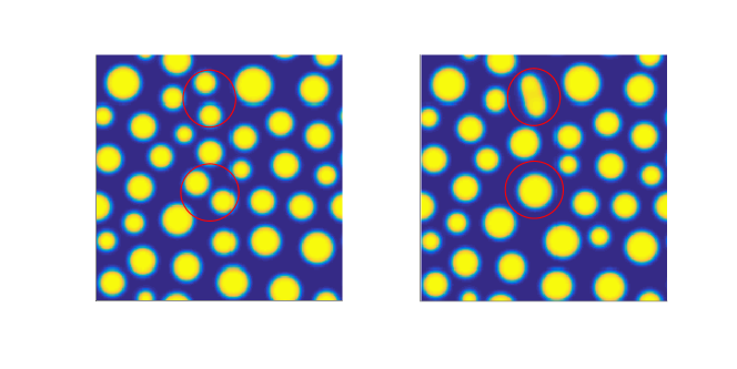
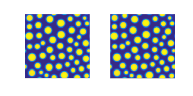
To illustrate the difference between two pressure expressions, we presented some results in Fig. 2. As seen in Fig. 2(a), the distributions of order parameter within the red circles are distinctly different, which means that the term $\Delta t(\tau_{g}-0.5)G_{0}$ in Eq. (25) has a significant influence on the numerical results. However, for incompressible LB model, there are no apparent differences, which is due to the fact that the effect of $\Delta t(\tau_{g}-0.5)G_{0}$ can be ignored when $S_{1}=0$, and $G_{0}$ is the order of $O(Ma^{2})$. Based on the above results, one can conclude that the pressure expression Eq. (25) is more general, and would be adopted in the following simulations.

Figure 2: (Colour online) Distribution of order parameter with Eq. (25) on the left, and Eq. (27) on the right, (a) the quasi-incompressible model at t=20000, (b) the incompressible model at t=20000.

4.2 Static droplet

A $2D$ static droplet is popular problem to verify LB models for two-phase flow [25, 50, 27, 36, 47]. In this subsection, we will consider this problem with different density ratios. Initially, a circular droplet with the radius ranging from $20$ to $40$ is placed in the middle of the computational domain with $NX\times NY=100\times 100$. The initial order parameter is given by

$$\phi(x,y)=0.5+0.5\tanh\frac{2\left[R-\sqrt{(x-50)^{2}+(y-50)^{2}}\right]}{W},$$ (64)

where $R$ is the droplet radius, and surface tension is expressed as $\mathbf{F_{s}}=-\phi\nabla\mu$. In numerical simulations, we set the density ratio to be $\rho_{A}/\rho_{B}=2,10$, and $50$. The other physical parameters are fixed as $\rho_{B}=1,\tau_{h}=1,\tau_{g}=0.8,\sigma=0.001,M_{\phi}=0.02$, and the periodic boundary conditions are applied at all boundaries. We first verify the LB model with the well-known Laplace’s law,

$$\Delta P=\frac{\sigma}{R},$$ (65)

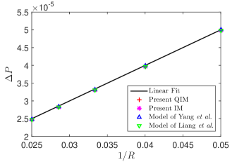
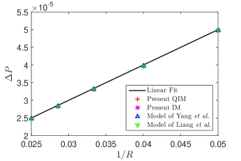
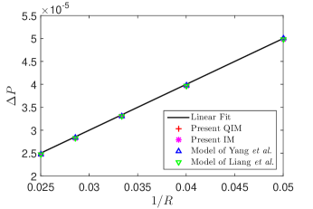
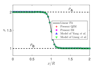
where $\Delta P$ is the pressure jump across the interface, $R$ is the radius of the droplet. $P$ is calculated by $P=p_{0}-\kappa\phi\nabla^{2}\phi+\kappa|\nabla\phi|^{2}/2+p$ with the equation of state $p_{0}=\phi\partial_{\phi}\psi-\psi$ [25, 51]. We performed some simulations and presented the results in Fig. 3. From Fig. 3(a), 3(c), 3(e) one can find that the results of present models and those in Refs. [27, 10] agree well with the Laplace law. In order to show the difference between these models more clearly, we also give the relative errors of pressure jump with the density ratio $\rho_{A}/\rho_{B}=50$ in Table 1. In general, the present quasi-incompressible LB model and quasi-incompressible model in Ref. [10] are more accurate than incompressible LB models. This is because that quasi-incompressible model is physically more reasonable than incompressible model. Besides, it is also found that usually present QIM is more accurate than the model in Ref. [10].

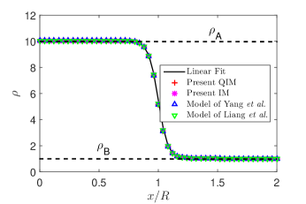
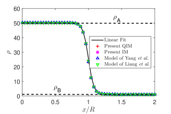
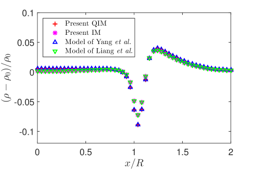
In addition, we also presented the density profiles along the horizontal center line at $t=5\times 10^{5}\Delta t$ in Figs. 3(b), 3(d), and 3(f). From these figures, one can observe that all the numerical results are very close to the analytical solutions given by Eq. (64). To give a quantitatively estimation on the accuracy of numerical results, we also measured the relative errors of density, i.e., [$(\rho-\rho_{0})/\rho_{0}$] with $\rho_{A}/\rho_{B}=10$ in Fig. 4(a), where $\rho_{0}$ is the analytical solution. Different from the results of Laplace’s law, we can find that the present incompressible LB models and the one in Ref. [27] produce smaller errors than quasi-incompressible models, which means that the quasi-incompressible and incompressible models each have their own advantages.

Figure 3: (Color online) Tests of Laplace’ law [(a), (c), (e)] and density profiles [(b), (d), (f)] at different density ratios ($\rho_{A}/\rho_{B}=2,10,50$), where the droplet radius is 25.

Table 1: Relative error of pressure jump with the density ratio $\rho_{A}/\rho_{B}=50$.

$R$			Present QIM	Present IM	Yang et al.	Liang et al.
20			$0.02\%$	$0.36\%$	$0.50\%$	$0.36\%$
25			$0.45\%$	$0.73\%$	$0.63\%$	$0.73\%$
30			$0.42\%$	$0.84\%$	$0.63\%$	$0.84\%$
35			$0.53\%$	$0.95\%$	$0.60\%$	$0.95\%$
40			$0.68\%$	$1.00\%$	$0.48\%$	$1.00\%$

Figure 4: (Color online) Tests of diffusion errors of density profiles with $\rho_{A}/\rho_{B}=10$ and $R=25$.

4.3 Layered Poiseuille flow

The layered Poiseuille flow between two parallel plates is also a classical two-phase problem which provides a good benchmark for validating the LB models [50, 25, 52, 38, 53, 31]. Considering a channel flow of two immiscible fluids driven by a const pressure gradient $G$ in the flowing direction ($x$-direction). Initially, fluid $A$ is located in the upper region of the channel ($0<y\leq h$), while fluid $B$ is at the bottom region ($-h\leq y\leq 0$). When the flow is sufficiently slow and no instabilities occur at the interface, an steady analytical solution of velocity can be obtained,

$$\mathbf{u}_{x,a}(y)=\left\{\begin{array}[]{l}\frac{Gh^{2}}{2\mu_{A}}\left[-\left(\frac{y}{h}\right)^{2}-\frac{y}{h}\left(\frac{\mu_{A}-\mu_{B}}{\mu_{A}+\mu_{B}}\right)+\frac{2\mu_{A}}{\mu_{A}+\mu_{B}}\right],\;\;\;\;\;0<y\leq h\\ \frac{Gh^{2}}{2\mu_{B}}\left[-\left(\frac{y}{h}\right)^{2}-\frac{y}{h}\left(\frac{\mu_{A}-\mu_{B}}{\mu_{A}+\mu_{B}}\right)+\frac{2\mu_{B}}{\mu_{A}+\mu_{B}}\right].\;\;\;-h\leq y\leq 0\\ \end{array}\right.$$ (66)

In this work, $G$ is given as $G=u_{c}(\mu_{A}+\mu_{B})/h^{2}$, and to ensure the stability of the interface, $u_{c}$ is fixed as $u_{c}=5\times 10^{-5}$. To quantitatively describe the accuracy of the present models and also convenient compare with the existing LB models, the following relative error is adopted [31],

$$Error=\frac{\sum\limits_{y}|u_{x}^{n}(y,t)-u_{x}^{a}(y)|}{\sum\limits_{y}|u_{x}^{a}(y)|},$$ (67)

where the subscripts $a$ and $n$ denote the analytical and numerical solutions.

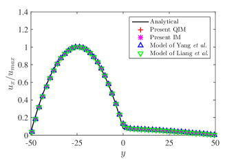
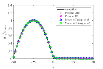
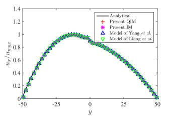
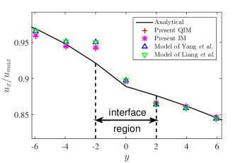
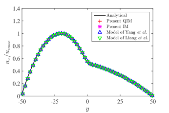
In our simulations, the computational domain is chosen as $NY\times NX=100\times 10$. Periodic boundary conditions are applied in the $x$-direction, and the halfway bounce-back boundary conditions are enforced on the top and bottom walls. We first investigated the effects of viscosity ratio. To this end, four different cases with viscosity ratios of $\mu_{A}/\mu_{B}=3,10,100,1000$ are considered. The other parameters are given as $W=4$, $\sigma=0.001$, $M_{\phi}=0.1$, $\rho_{l}/\rho_{g}=1$. Based on the results in Fig. 5, one can find that the numerical results of present LB models and some others [10, 27] agree well with the analytical solutions for different viscosity ratios. We also calculated the relative errors of velocity under different viscosity ratios, and the results are given in Table 2. From this table, one can observe that the relative error increases as the viscosity ratio becomes larger, and for a fixed viscosity ratio, the relative errors of all these models are almost the same. This is because if the density ratios are equal to $1$, which leads to $\gamma=0$, the quasi-incompressible and incompressible models are equivalent except for some terms with the order of $O(Ma^{2})$.

We then simulated the layered Poiseuille flow with another density ratio $\rho_{A}/\rho_{B}=3$, and viscosity ratio is equal to $3$. Here the dynamic viscosity is given by [35, 31]

$$\mu=\left\{\begin{array}[]{l}\mu_{A},\;\;\;\;\;\phi\geq 0.5,\\ \mu_{B},\;\;\;\;\;\phi<0.5.\\ \end{array}\right.$$ (68)

The other parameters are the same as those stated above. From Fig. 6(a), one can find that there is a good agreement between the numerical solutions of the four LB models and the analytical solutions except in the interface region. Fig. 6(b) is an enlarged view of the interface region in Fig. 6(a). From this figure, it can be observed that the present QIM and IM produce smaller errors than the models of Yang et al. [10] and Liang et al. [27] in the interface area, while their models are more accurate in the bulk region. In other words, our models have a better performance in the interface region, in contrast, the models of Yang et al. [10] and Liang et al. [27] are more accurate in the bulk region.

Figure 5: (Color online) Comparison of the velocity distributions obtained by present QIM, IM, model of Yang et al. [10], and model of Liang et al. [27] with the corresponding analytical solutions (solid line): (a) $\mu_{A}/\mu_{B}=3$, (b) $\mu_{A}/\mu_{B}=10$, (c) $\mu_{A}/\mu_{B}=100$, (d) $\mu_{A}/\mu_{B}=1000$. $u_{x}$ is normalized by he maximum speed of analytical solution $u_{max}$.

Table 2: Relative errors of velocity for different viscosity ratios.

Models	$\frac{\mu_{A}}{\mu_{B}}=3$	$\frac{\mu_{A}}{\mu_{B}}=10$	$\frac{\mu_{A}}{\mu_{B}}=100$	$\frac{\mu_{A}}{\mu_{B}}=1000$
Present QIM	$1.04\%$	$1.30\%$	$1.90\%$	$2.16\%$
Present IM	$1.04\%$	$1.30\%$	$1.90\%$	$2.16\%$
Yang et al. [10]	$1.04\%$	$1.30\%$	$1.90\%$	$2.16\%$
Liang et al. [27]	$1.04\%$	$1.30\%$	$1.90\%$	$2.16\%$

Figure 6: (Color online) Comparison of the velocity distributions obtained by present QIM, IM, model of Yang et al. [10], and model of Liang et al. [27] with the analytical solution (solid line), where $\rho_{A}/\rho_{B}=3$, and $\mu_{A}/\mu_{B}=3$: (a) velocity distribution in the whole region, (b) velocity distribution in the interface region.

4.4 Bubble rising under buoyancy

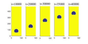
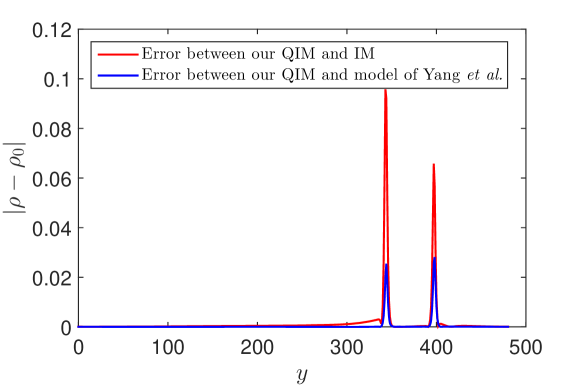
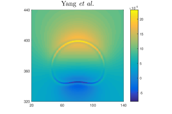
To further demonstrate the accuracy of the present models for more complex flows, the problem of single bubble rising flow driven by the buoyancy is also considered here. Initially, a circular bubble (fluid B) without initial velocity is immersed in the bottom center of another fluid (A). The radius of the initial bubble, $R$, occupies $32$ lattice spaces. To generate the buoyancy effects, a body force, $F_{b,y}=-(\rho-\rho_{A})g$, is added to the momentum equation, where $g$ is the gravitational acceleration. We conducted some simulations on a uniform computational mesh with the size of $NX\times NY=160\times 480$, and the periodic boundary conditions are applied at all boundaries. The other related parameters are given as $W=4,g=10^{-5},\sigma=0.001,\tau_{f}=\tau_{g}=1,M_{\phi}=6.667,\rho_{A}/\rho_{B}=2$. Fig. 7 shows the density distributions of the rising bubble at different times based on our models and models of Yang et al. [10] and Liang et al. [27]. From this figure, it can be observed that the results of these models are quite similar to each other. However, a zoom-in-view of Fig. 7 at $t=40000$ shows that the incompressible models (our IM and Liang’s model) will produce numerical oscillation near the interface region (see Fig. 8). To see the differences among these LB models more clearly, we show the errors along the vertical centerline at $t=40000$ in Fig. 9, where the error between our QIM and IM increases sharply to $0.096$ near the interface. This phenomenon is reasonable because the compressible term $\gamma\nabla\cdot(M_{\phi}\nabla\mu)$ has an influence on the numerical results. While, the maximum error between our QIM and the one in Ref. [10] is approximately $0.028$, which is caused by the difference between the two models. In the model of Yang et al. [10], the N-S equations in artificial compressible form can be derived. To neglect the artificial compressible effect, the condition $T\gg L/c_{s}$ should be satisfied. While from present QIM, the quasi-incompressible N-S equations can be exactly recovered in the limit of a low Mach number.

Figure 7: (Color online) Density distributions of the rising bubble at $t=10000,20000,30000,35000,40000$, (a) present QIM, (b) present IM, (c) model of Yang et al. [10], and (d) model of Liang et al. [27].

Figure 8: (Color online) The enlarged images of density distributions of the rising bubble at $t=40000$ for present QIM, present IM, model of Yang et al. [10], and model of Liang et al. [27].

Figure 9: (Color online) Errors along the vertical centerline at $t=40000$, where $\rho_{0}$ is the result of our QIM.

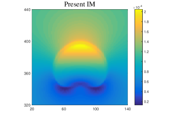
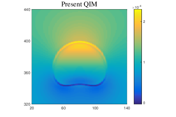
Fig. 10 depicts the pressure distributions of the rising bubble at $t=40000$ based on different models. From this figure, one can see that there is a significant difference between quasi-incompressible models and incompressible models, and the pressure interface of quasi-incompressible models is clearer.

Based on above observations, one can conclude that quasi-incompressible models (our QIM and Liang’s model) are more superior for complex two-phase flows.

Figure 10: (Color online) Pressure distributions of the rising bubble at $t=40000$ for (a) present QIM, (b) present IM, (c) model of Yang et al. [10], and (d) model of Liang et al.. [27]

5 Conclusions

In this study, to solve single-phase flow problems with a mass source term in the governing equations and other problems coupled with the flow field, such as two-phase flow problems, we developed a generalized LB model for incompressible and nearly incompressible N-S equations with a mass source term. The proposed model not only contains some existing models, but also extends them. From the generalized model, we can not only get some existing models, but also derive new models. Among these derived models, we can get an incompressible model for N-S equations with a mass source term, and we present a modified scheme to calculate the pressure $p$, which is more accurate than the previous one. Simultaneously, our generalized model can recover the macroscopic equations without any unnecessary assumptions. Based on the generalized LB model, a new LB model is proposed for the quasi-incompressible and incompressible phase-field system. To validate the accuracy of the proposed model, a series of numerical tests were performed.

First, we conducted a detailed comparison between present scheme and the previous one [27, 31, 35]. The result shows that there is a significant difference between the two pressure schemes when $S_{1}\neq 0$, and theoretically, the present pressure scheme is more accurate. Then we investigated two basic steady problems of a static droplet and layered Poiseuille flows. The results of the former case show that present quasi-incompressible model usually performs better than the quasi-incompressible model of Yang et al. [10] in terms of accuracy, and quasi-incompressible models are more accurate than incompressible models. In the latter case, we simulated the layered Poiseuille flows with $\rho_{A}/\rho_{B}=1$ and $\rho_{A}/\rho_{B}\neq 1$, and found that our models can obtain satisfactory results in the velocity under different viscosity ratios, and our models have a better performance in the interface region when $\rho_{A}/\rho_{B}\neq 1$. Finally, we carried out some simulations of single bubble rising flow driven by the buoyancy to further demonstrate the accuracy of the present models. The results indicate that the incompressible LB models will produce numerical oscillation near the interface region. While, the quasi-incompressible LB models seem more reasonable from physical point of view, and should be considered in the study of complex two-phase flows.

Appendix A Chapman-Enskog analysis of the present model

In the Appendix A, we would present the details on how to obtain the proposed LB model for hydrodynamic equations [Eq. (5b)] through the Chapman-Enskog (C-E) expansion.

Before performing C-E expansion, we first define the zeroth to second moments of the equilibrium distribution function,

$$\sum_{i}g_{i}^{eq}=M_{0},\sum_{i}\mathbf{c}_{i}g_{i}^{eq}=M_{1},\sum_{i}\mathbf{c}_{i}\mathbf{c}_{i}g_{i}^{eq}=M_{2},\sum_{i}\mathbf{c}_{i}\mathbf{c}_{i}\mathbf{c_{i}}g_{i}^{eq}=M_{3}.$$ (69)

In the C-E analysis, the time and space derivatives, the force and source term can be expanded as,

$$g_{i}=g_{i}^{(0)}+\epsilon g_{i}^{(1)}+\epsilon^{2}g_{i}^{(2)}+\cdots,$$ (70a)

$$G_{i}=\epsilon G_{i}^{(1)}+\epsilon^{2}G_{i}^{(2)},$$ (70b)

$$\partial_{t}=\epsilon\partial_{t_{1}}+\epsilon^{2}\partial_{t_{2}},\partial_{\alpha}=\epsilon\partial_{1\alpha},$$ (70c)

$$F_{\alpha}=\epsilon F_{\alpha}^{(1)}+\epsilon^{2}F_{\alpha}^{(2)},$$ (70d)

$$S=\epsilon S^{(1)}+\epsilon^{2}S^{(2)},$$ (70e)

where $\epsilon$ is a small expansion parameter and Greek indices denote Cartesian spatial components. Using the Taylor expansion to Eq. (15), we have

$$\Delta tD_{i}g_{i}(\textbf{x},t)+\frac{\Delta t^{2}}{2}D_{i}^{2}g_{i}(\textbf{x},t)+\cdots=-\frac{1}{\tau_{g}}\left(g_{i}(\mathbf{x},t)-g_{i}^{eq}(\mathbf{x},t)\right)+\Delta t(1-\frac{1}{2\tau_{g}})G_{i},$$ (71)

where $D_{i}=\partial_{t}+c_{i\alpha}\partial_{\alpha}$, and substituting Eq. (70e) into Eq. (71), one can obtain the following multi-scale equations,

$$O(\epsilon^{0}):g_{i}^{(0)}=g_{i}^{eq},$$ (72a)

$$O(\epsilon^{1}):D_{1i}g_{i}^{(0)}=-\frac{1}{\tau_{g}\Delta t}g_{i}^{(1)}+(1-\frac{1}{2\tau_{g}})G_{i}^{(1)},$$ (72b)

$$O(\epsilon^{2}):\partial_{t_{2}}g_{i}^{(0)}+D_{1i}g_{i}^{(1)}+\frac{\Delta t}{2}D_{1i}^{2}g_{i}^{(0)}=-\frac{1}{\tau_{g}\Delta t}g_{i}^{(2)}+(1-\frac{1}{2\tau_{g}})G_{i}^{(2)},$$ (72c)

where $D_{1i}=\partial_{t_{1}}+c_{i\alpha}\partial_{1\alpha}$.

Then, the substitution of Eq. (72b) into Eq. (72c) yields

$$\partial_{t_{2}}g_{i}^{(0)}+(1-\frac{1}{2\tau_{g}})D_{1i}g_{i}^{(1)}+\frac{\Delta t}{2}(1-\frac{1}{2\tau_{g}})D_{1i}G_{i}^{(1)}=-\frac{1}{\tau_{g}\Delta t}g_{i}^{(2)}+(1-\frac{1}{2\tau_{g}})G_{i}^{(2)}.$$ (73)

By summing Eq. (72b) and Eq. (72b)$\times c_{i\beta}$ over $i$, the recovered equations at $\epsilon$ scale can be obtained,

$$\partial_{t_{1}}M_{0}+\partial_{1\alpha}M_{1\alpha}=-\frac{1}{\tau_{g}\Delta t}\sum_{i}g_{i}^{(1)}+(1-\frac{1}{2\tau_{g}})\sum_{i}G_{i}^{(1)},$$ (74a)

$$\partial_{t_{1}}M_{1\beta}+\partial_{1\alpha}M_{2\alpha\beta}=-\frac{1}{\tau_{g}\Delta t}\sum_{i}c_{i\beta}g_{i}^{(1)}+(1-\frac{1}{2\tau_{g}})\sum_{i}c_{i\beta}G_{i}^{(1)}.$$ (74b)

Similarly, we can also obtain the recovered equations at $\epsilon^{2}$ scale from Eq. (73)

$$\begin{split}&\partial_{t_{2}}M_{0}+(1-\frac{1}{2\tau_{g}})\left[\partial_{t_{1}}(\sum_{i}g_{i}^{(1)})+\partial_{1\alpha}(\sum_{i}c_{i\alpha}g_{i}^{(1)})\right]+\frac{\Delta t}{2}(1-\frac{1}{2\tau_{g}})\left[\partial_{t_{1}}(\sum_{i}G_{i}^{(1)})+\right.\\ &\left.\partial_{1\alpha}(\sum_{i}c_{i\alpha}G_{i}^{(1)})\right]=-\frac{1}{\tau_{g}\Delta t}\sum_{i}g_{i}^{(2)}+(1-\frac{1}{2\tau_{g}})\sum_{i}G_{i}^{(2)},\end{split}$$ (75a)

$$\begin{split}&\partial_{t_{2}}M_{1\beta}+(1-\frac{1}{2\tau_{g}})\left[\partial_{t_{1}}(\sum_{i}c_{i\beta}g_{i}^{(1)})+\partial_{1\alpha}\Lambda^{(1)}\right]+\frac{\Delta t}{2}(1-\frac{1}{2\tau_{g}})\left[\partial_{t_{1}}(\sum_{i}c_{i\beta}G_{i}^{(1)})+\right.\\ &\left.\partial_{1\alpha}(\sum_{i}c_{i\alpha}c_{i\beta}G_{i}^{(1)})\right]=-\frac{1}{\tau_{g}\Delta t}\sum_{i}c_{i\beta}g_{i}^{(2)}+(1-\frac{1}{2\tau_{g}})\sum_{i}c_{i\beta}G_{i}^{(2)},\end{split}$$ (75b)

where $\Lambda^{(1)}=\sum_{i}c_{i\alpha}c_{i\beta}g_{i}^{(1)}$ is the first-order momentum flux tensor.

Summing Eq. (14) and Eq. (14)$\times c_{i\alpha}$ over $i$, one can obtain

$$M_{0}=\sum_{i}g_{i}+\frac{\Delta t}{2}\sum_{i}G_{i},$$ (76a)

$$M_{1\alpha}=\sum_{i}c_{i\alpha}g_{i}+\frac{\Delta t}{2}\sum_{i}c_{i\alpha}G_{i},$$ (76b)

which can be further recast as

$$\sum_{i}g_{i}^{(1)}=-\frac{\Delta t}{2}\sum_{i}G_{i}^{(1)},\sum_{i}g_{i}^{(2)}=-\frac{\Delta t}{2}\sum_{i}G_{i}^{(2)},$$ (77a)

$$\sum_{i}c_{i\alpha}g_{i}^{(1)}=-\frac{\Delta t}{2}\sum_{i}c_{i\alpha}G_{i}^{(1)},\sum_{i}c_{i\alpha}g_{i}^{(2)}=-\frac{\Delta t}{2}\sum_{i}c_{i\alpha}G_{i}^{(2)}.$$ (77b)

Substituting Eq. (77b) into Eqs. (74b) and (75b), we have

$$\partial_{t_{1}}M_{0}+\partial_{1\alpha}M_{1\alpha}=\sum_{i}G_{i}^{(1)},$$ (78a)

$$\partial_{t_{1}}M_{1\beta}+\partial_{1\alpha}M_{2\alpha\beta}=\sum_{i}c_{i\beta}G_{i}^{(1)},$$ (78b)

$$\partial_{t_{2}}M_{0}=\sum_{i}G_{i}^{(2)},$$ (79a)

$$\partial_{t_{2}}M_{1\beta}+(1-\frac{1}{2\tau_{g}})\partial_{1\alpha}\Lambda^{(1)}+\frac{\Delta t}{2}(1-\frac{1}{2\tau_{g}})\partial_{1\alpha}(\sum_{i}c_{i\alpha}c_{i\beta}G_{i}^{(1)})=\sum_{i}c_{i\beta}G_{i}^{(2)}.$$ (79b)

Combining Eq. (78a) and Eq. (79a) at $\epsilon$ and $\epsilon^{2}$ scales yields

$$\partial_{t}M_{0}+\partial_{1\alpha}M_{1\alpha}=\sum_{i}G_{i}.$$ (80)

To recover the continuity equation with a source term [Eq. (5a)], the following conditions should be satisfied

$$M_{0}=\tilde{\rho},M_{1}=\rho\mathbf{u},\sum_{i}G_{i}=S.$$ (81)

In addition, to recover the momentum equation [Eq. (5b)], $M_{2}=p\mathbf{I}+\rho\mathbf{uu}$ is also needed. Thus, the equilibrium distribution function can be given as

$$g_{i}^{eq}=\left\{\begin{array}[]{l}\tilde{\rho}+\frac{p}{c_{s}^{2}}(\omega_{i}-1)+\rho s_{i}(\mathbf{u}),\;\;\;i=0,\\ \frac{p}{c_{s}^{2}}\omega_{i}+\rho s_{i}(\mathbf{u}),\;\;\;\;\;\;\;\;\;\;\;\;\;\;\;\;\;i\neq 0,\end{array}\right.$$ (82)

and Eq. (78b) can be rewritten as

$$\partial_{t_{1}}(\rho u_{\beta})+\partial_{1\beta}p+\partial_{1\alpha}(\rho u_{\alpha}u_{\beta})=\sum_{i}c_{i\beta}G_{i}^{(1)}.$$ (83)

To derive the equation at $\epsilon^{2}$ scale, we first express $\Lambda^{(1)}$ as

$$\begin{split}\Lambda^{(1)}&=-\tau_{g}\Delta t\left[\partial_{t_{1}}M_{2\alpha\beta}+\partial_{1\gamma}M_{3\alpha\beta\gamma}-(1-\frac{1}{2\tau_{g}})\sum_{i}c_{i\alpha}c_{i\beta}G_{i}^{(1)}\right]\\ &=-\tau_{g}\Delta t\left\{\partial_{t_{1}}p\delta_{\alpha\beta}+\partial_{t_{1}}(\rho u_{\alpha}u_{\beta})+c_{s}^{2}\partial_{1\gamma}(\rho u_{\gamma}\delta_{\alpha\beta})+c_{s}^{2}\partial_{1\gamma}[\rho(u_{\alpha\delta_{\beta\gamma}}+u_{\beta}\delta_{\alpha\gamma})]\right.\\ &\left.\quad-(1-\frac{1}{2\tau_{g}})\sum_{i}c_{i\alpha}c_{i\beta}G_{i}^{(1)}\right\},\end{split}$$ (84)

where Eq. (72b) has been used, and the term $\partial_{t_{1}}(\rho u_{\alpha}u_{\beta})$ can be given by

$$\partial_{t_{1}}(\rho u_{\alpha}u_{\beta})=u_{\alpha}(\sum_{i}c_{i\beta}G_{i}^{(1)})+u_{\beta}(\sum_{i}c_{i\alpha}G_{i}^{(1)})-(u_{\alpha}\partial_{1\beta}p+u_{\beta}\partial_{1\alpha}p)-u_{\alpha}u_{\beta}\tilde{S}^{(1)},$$ (85)

where the Eqs. (83) and Eq. (78a) are used, $\tilde{S}^{(1)}=S^{(1)}+\partial_{t_{1}}(\rho-\tilde{\rho})$ and the term of $O(Ma^{3})$ has been neglected.

Combining Eq. (83) with Eq. (79b) at $\epsilon$ and $\epsilon^{2}$ scales, together with Eq. (84) and Eq. (85), we now obtain

$$\begin{split}\partial_{t}(\rho u_{\beta})+\partial_{\alpha}(\rho u_{\alpha}u_{\beta})=&-\partial_{\beta}p+\partial_{\alpha}\left[\rho\nu(\partial_{\alpha}u_{\beta}+\partial_{\beta}u_{\alpha})\right]+\epsilon\Delta t(\tau_{g}-0.5)\partial_{\alpha}\left[\partial_{t_{1}}p\delta_{\alpha\beta}\right.\\ &+\partial_{1\gamma}(c_{s}^{2}\rho u_{\gamma}\delta_{\alpha\beta})+u_{\alpha}(\sum_{i}c_{i\beta}G_{i}^{(1)})+u_{\beta}(\sum_{i}c_{i\alpha}G_{i}^{(1)})+\\ &c_{s}^{2}(u_{\alpha}\partial_{1\beta}\rho+u_{\beta}\partial_{1\alpha}\rho)-(u_{\alpha}\partial_{1\beta}p+u_{\beta}\partial_{1\alpha}p)-u_{\alpha}u_{\beta}\tilde{S}^{(1)}\\ &\left.-\sum_{i}c_{i\alpha}c_{i\beta}G_{i}^{(1)}\right]+\sum_{i}c_{i\beta}G_{i}.\end{split}$$ (86)

where the kinetic viscosity is determined by

$$\nu=c_{s}^{2}(\tau_{g}-0.5)\Delta t.$$ (87)

Compared to Eq. (5b), we can recover the momentum equation as long as the following equations hold,

$$\sum_{i}c_{i\beta}G_{i}=F_{\beta},$$ (88)

$$\begin{split}\sum_{i}c_{i\alpha}c_{i\beta}G_{i}=&\partial_{t}p\delta_{\alpha\beta}+\partial_{\gamma}(c_{s}^{2}\rho u_{\gamma}\delta_{\alpha\beta})+u_{\alpha}F_{\beta}+u_{\beta}F_{\alpha}+c_{s}^{2}(u_{\alpha}\partial_{\beta}\rho+u_{\beta}\partial_{\alpha}\rho)-\\ &(u_{\alpha}\partial_{\beta}p+u_{\beta}\partial_{\alpha}p)-u_{\alpha}u_{\beta}\tilde{S}+\left(\frac{2}{d}\rho c_{s}^{2}-\frac{\xi}{\Delta t(\tau_{g}-0.5)}\right)\partial_{\gamma}u_{\gamma}\delta_{\alpha\beta}.\end{split}$$ (89)

Based on Eqs. (88), (89), and the last equation in Eq. (81), the force distribution function can be given by

$$G_{i}=\omega_{i}\left\{S+\frac{\mathbf{c}_{i}\cdot\mathbf{F}}{c_{s}^{2}}+\frac{(\mathbf{c}_{i}\mathbf{c}_{i}-c_{s}^{2}\mathbf{I}):\left[\partial_{t}(p-\tilde{\rho}c_{s}^{2})\mathbf{I}+\mathbf{u\tilde{F}}+\mathbf{\tilde{F}u}-\mathbf{uu}\tilde{S}+Q(\nabla\cdot\mathbf{uI})\right]}{2c_{s}^{4}}\right\},$$ (90)

where $\tilde{F}$ is a modified total force

$$\mathbf{\tilde{F}}=\mathbf{F}-\nabla(p-\rho c_{s}^{2}),$$ (91)

$\tilde{S}$ and $Q$ can be expressed as

$$\tilde{S}=S+\partial_{t}(\rho-\tilde{\rho}).$$ (92)

$$Q=\frac{2}{d}{\rho}c_{s}^{2}-\frac{\xi}{\Delta t(\tau_{g}-0.5)}.$$ (93)

Appendix B The computation of the pressure

Now we will focus on how to calculate the pressure from the distribution function $g_{i}$. According to the expression of $g_{0}^{eq}$, we have

$$\frac{p}{c_{s}^{2}}(1-\omega_{0})=\tilde{\rho}+\rho s_{0}(\mathbf{u})-g_{0}^{eq}.$$ (94)

Actually, once $g_{0}^{eq}$ in Eq. (94) is replaced by the distribution function $g_{i}$, one can present a scheme to calculate pressure. Firstly, from Eq. (72b) we can derive

$$\epsilon g_{i}^{(1)}=-\epsilon\tau_{g}\Delta t\left[D_{1i}g_{i}^{(0)}-(1-\frac{1}{2\tau_{g}})G_{i}^{(1)}\right]+O(\Delta t^{2}),$$ (95)

or equivalently,

$$g_{i}-g_{i}^{eq}=-\epsilon\tau_{g}\Delta t\left[D_{1i}g_{i}^{(0)}-(1-\frac{1}{2\tau_{g}})G_{i}^{(1)}\right]+O(\Delta t^{2}).$$ (96)

Taking the zeroth-direction of Eq. (96), we have

$$\begin{split}g_{0}-g_{0}^{eq}&=-\epsilon\tau_{g}\Delta t\left[\partial_{t_{1}}g_{0}^{(0)}-(1-\frac{1}{2\tau_{g}})G_{0}^{(1)}\right]+O(\Delta t^{2})\\ &=-\tau_{g}\Delta t\left[\partial_{t}g_{0}^{(0)}-(1-\frac{1}{2\tau_{g}})G_{0}\right]+O(\Delta t^{2}).\end{split}$$ (97)

Note that the term $\partial_{t}g_{0}^{(0)}$ is the order of $O(Ma^{2})$, thus, we get

$$-g_{0}^{eq}=-g_{0}+\tau_{g}\Delta t(1-\frac{1}{2\tau_{g}})G_{0}+O(\Delta t^{2}+\Delta tMa^{2}).$$ (98)

Neglecting the terms of $O(\Delta t^{2}+\Delta tMa^{2})$, and substituting Eq. (98) into Eq. (94), we can obtain

$$\begin{split}\frac{p}{c_{s}^{2}}(1-\omega_{0})&=\tilde{\rho}+\rho s_{0}(\mathbf{u})-g_{0}+\Delta t(\tau-\frac{1}{2})G_{0}\\ &=\tilde{\rho}+\rho s_{0}(\mathbf{u})-(\sum_{i}g_{i}-\sum_{i\neq 0}g_{i})+\Delta t(\tau-\frac{1}{2})G_{0}\\ &=\tilde{\rho}+\rho s_{0}(\mathbf{u})-(\sum_{i}g_{i}^{eq}-\frac{\Delta t}{2}\sum_{i}G_{i}-\sum_{i\neq 0}g_{i})+\Delta t(\tau-\frac{1}{2})G_{0}\\ &=\tilde{\rho}+\rho s_{0}(\mathbf{u})-\tilde{\rho}+\frac{\Delta t}{2}S+\sum_{i\neq 0}g_{i}+\Delta t(\tau-\frac{1}{2})G_{0}\\ &=\rho s_{0}(\mathbf{u})+\frac{\Delta t}{2}S+\sum_{i\neq 0}g_{i}+\Delta t(\tau-\frac{1}{2})G_{0}.\end{split}$$ (99)

As a result, the pressure can be calculated as

$$p=\frac{c_{s}^{2}}{1-\omega_{0}}\left[\sum_{i\neq 0}g_{i}+\frac{\Delta t}{2}S+\rho s_{0}(\mathbf{u})+\Delta t(\tau-\frac{1}{2})G_{0}\right],$$ (100)

which has an accuracy of $O(\Delta t^{2}+\Delta tMa^{2})$.

References

• [1] G. Tryggvason, B. Bunner, A. Esmaeeli, et al. A front-tracking method for the computations of multiphase flow. J. Comput. Phys, 2001, 169(2): 708-759.
• [2] X. He, S. Chen, and R. Zhang. A lattice Boltzmann scheme for incompressible multiphase flow and its application in simulation of Rayleigh-Taylor instability. J. Comput. Phys, 1999, 152(2): 642-663.
• [3] T. Ramstad, P. E. ร˜ren, and S. Bakke. Simulation of two-phase flow in reservoir rocks using a lattice Boltzmann method. SPE J, 2010, 15(04): 917-927.
• [4] O. Aursjรธ, and S. R. Pride. Lattice Boltzmann method for diffusion-limited partial dissolution of fluids. Phys. Rev. E, 2015, 92(1): 013306.
• [5] F. Jiang and T. Tsuji. Estimation of three-phase relative permeability by simulating fluid dynamics directly on rock-microstructure images. Water Resour. Res, 2017, 53(1): 11-32.
• [6] H. Liang, B. C. Shi, and Z. H. Chai. Lattice Boltzmann modeling of three-phase incompressible flows. Phys. Rev. E, 2016, 93(1): 013308.
• [7] K. Vafai, and C. L. Tien. Boundary and inertia effects on flow and heat transfer in porous media. Int. J. Heat Mass Transf, 1981, 24(2): 195-203.
• [8] Y. Peng, C. Shu, and Y. T. Chew. Simplified thermal lattice Boltzmann model for incompressible thermal flows. Phys. Rev. E, 2003, 68(2): 026701.
• [9] C. Pan, M. Hilpert, and C. Miller. Lattice-Boltzmann simulation of two-phase flow in porous media. Water Resour. Res, 2004, 40(1).
• [10] K. Yang, Z. L. Guo. Lattice Boltzmann method for binary fluids based on mass-conserving quasi-incompressible phase-field theory. Phys. Rev. E, 2016, 93(4): 043303.
• [11] J. Shen, X. Yang, and Q. Wang. Mass and volume conservation in phase field models for binary fluids. Commun. Comput. Phys, 2013, 13(4): 1045-1065.
• [12] O. Aursjรธ, E. Jettestuen, J. L. Vinningland, and A. Hiorth. On the inclusion of mass source terms in a single-relaxation-time lattice Boltzmann method. Phys. Fluids, 2018, 30(5): 057104.
• [13] A. Kuzmin, Z. L. Guo, and A. A. Mohamad. Simultaneous incorporation of mass and force terms in the multi-relaxation-time framework for lattice Boltzmann schemes. Philosophical Transactions of the Royal Society of London A: Mathematical, Phil. Trans. R. Soc, 2011, 369(1944): 2219-2227.
• [14] C. T. Crowe, M. P. Sharma, and D. E. Stock. The particle-source-in cell (PSI-CELL) model for gas-droplet flows. J. Fluids Eng, 1977, 99(2): 325-332.
• [15] D. Migdal, and V. D. Agosta. A source flow model for continuum gas-particle flow[J]. J. Appl. Mech, 1967, 34: 860.
• [16] S. Dutta, S. Shimpalee, and J. W. V. Zee. Numerical prediction of mass-exchange between cathode and anode channels in a PEM fuel cell. Int. J. Heat Mass Transf, 2001, 44(11): 2029-2042.
• [17] T. Krรผger, H. Kusumaatmaja, G. Silva, O. Shardt, A. Kuzmin and E.M. Viggen. The Lattice Boltzmann Method: Principles and Practice (Springer International Publishing, Switzerland, 2017).
• [18] Z. H. Chai, B. C. Shi, and Z. L. Guo. A multiple-relaxation-time lattice Boltzmann model for general nonlinear anisotropic convection-diffusion equations. J. Sci. Comput, 2016, 69(1): 355-390.
• [19] X. He and G. Doolen. Lattice Boltzmann method on curvilinear coordinates system: flow around a circular cylinder. J. Comput. Phys, 1997, 134(2): 306-315.
• [20] Z. L. Guo, B. C. Shi, and N. C. Wang. Lattice BGK model for incompressible Navier-Stokes equation. J. Comput. Phys, 2000, 165(1): 288-306.
• [21] C. K. Aidun and J. R. Clausen. Lattice-Boltzmann method for complex flows. Annu. Rev. Fluid. Mech, 2010, 42: 439-472.
• [22] H. Liang, Y. Li, J. X. Chen, and J. R. Xu. Axisymmetric lattice Boltzmann model for multiphase flows with large density ratio. Int. J. Heat Mass Transf, 2019, 130: 1189-1205.
• [23] I. Halliday, L. Hammond, C. Care, K. Good, and A. Stevens. Lattice Boltzmann equation hydrodynamics. Phys. Rev. E, 2001, 64(1): 011208.
• [24] Y. Cheng and J. Li. Introducing unsteady non-uniform source terms into the lattice Boltzmann model. Int. J. Numer. Methods Fluids, 2008, 56(6): 629-641.
• [25] Y. Q. Zu and S. He. Phase-field-based lattice Boltzmann model for incompressible binary fluid systems with density and viscosity contrasts. Phys. Rev. E, 2013, 87(4): 043301.
• [26] H. W. Zheng, C. Shu, and Y. T. Chew. Lattice Boltzmann interface capturing method for incompressible flows. Phys. Rev. E, 2005, 72(5): 056705.
• [27] H. Liang, B. C. Shi, Z. L. Guo, and Z. H. Chai. Phase-field-based multiple-relaxation-time lattice Boltzmann model for incompressible multiphase flows. Phys. Rev. E, 2014, 89(5): 053320.
• [28] C. H. Zhang, K. Yang, and Z. L. Guo, Int. J. Heat Mass Transf. 126, 1326 (2018).
• [29] D. Jacqmin. Calculation of two-phase Navier-Stokes flows using phase-field modeling. J. Comput. Phys, 1999, 155(1): 96-127..
• [30] S. O. Unverdi and G. Tryggvason. A front-tracking method for viscous, incompressible, multi-fluid flows. J. Comput. Phys, 1992, 100(1): 25-37.
• [31] H. Liang, J. R. Xu, J. X. Chen, H. L. Wang, Z. H. Chai, and B. C. Shi. Phase-field-based lattice Boltzmann modeling of large-density-ratio two-phase flows. Phys. Rev. E, 2018, 97(3): 033309.
• [32] G. Emanuel. Bulk viscosity in the Navier-Stokes equations. Int. J. Eng. Sci, 1998, 36(11): 1313-1323.
• [33] L. S. Luo. Unified theory of lattice Boltzmann models for nonideal gases. Phys. Rev. Lett, 1998, 81(8): 1618.
• [34] R. Du and B. C. Shi. A novel scheme for force term in the lattice BGK model. Int. J. Mod. Phys. C, 2006, 17(07): 945-958.
• [35] F. Ren, B. W. Song, M. C. Sukop, and H. B. Hu. Improved lattice Boltzmann modeling of binary flow based on the conservative Allen-Cahn equation. Phys. Rev. E, 2016, 94(2): 023311.
• [36] T. Lee and C. L. Lin. A stable discretization of the lattice Boltzmann equation for simulation of incompressible two-phase flows at high density ratio. J. Comput. Phys, 2005, 206(1): 16-47.
• [37] T. Lee and L. Liu. Lattice Boltzmann simulations of micron-scale drop impact on dry surfaces. J. Comput. Phys, 2010, 229(20): 8045-8063.
• [38] A. Fakhari and D. Bolster. Diffuse interface modeling of three-phase contact line dynamics on curved boundaries: A lattice Boltzmann model for large density and viscosity ratios. J. Comput. Phys, 2017, 334: 620-638.
• [39] X. He, Q. Zou, and L.-S. Luo. Analytic solutions of simple flows and analysis of nonslip boundary conditions for the lattice Boltzmann BGK model. J. Stat. Phys, 1997, 87(1-2): 115-136.
• [40] V. M. Kendon, M. E. Cates, I. Pagonabarraga, J. C. Desplat, and P. Bladon. Inertial effects in three-dimensional spinodal decomposition of a symmetric binary fluid mixture: a lattice Boltzmann study. J. Fluid Mech, 2001, 440: 147-203.
• [41] V. E. Bandalassi, H. D. Ceniceros, and S. Banerjee. Computation of multiphase systems with phase field models. J. Comput. Phys, 2003, 190(2): 371-397.
• [42] D. Jacqmin. Contact-line dynamics of a diffuse fluid interface. J. Fluid Mech, 2000, 402: 57-88.
• [43] Y. Y. Yan and Y. Q. Zu. A lattice Boltzmann method for incompressible two-phase flows on partial wetting surface with large density ratio. J. Comput. Phys, 2007, 227(1): 763-775.
• [44] Z. Chai, D. Sun, H. Wang, and B. Shi. A comparative study of local and nonlocal Allen-Cahn equations with mass conservation. Int. J. Heat Mass Transf, 2018, 122: 631-642.
• [45] H. W. Zheng, C. Shu, and Y. T. Chew. A lattice Boltzmann model for multiphase flows with large density ratio. J. Comput. Phys, 2006, 218(1): 353-371.
• [46] J. J. Huang, C. Shu, and Y. T. Chew, Int. J. Numer. Methods Fluids 60, 203 (2009).
• [47] A. Fakhari and M. H. Rahimian. Phase-field modeling by the method of lattice Boltzmann equations. Phys. Rev. E, 2010, 81(3): 036707.
• [48] Z. H. Chai and T. S. Zhao. Lattice Boltzmann model for the convection-diffusion equation. Phys. Rev. E, 2013, 87(6): 063309.
• [49] J. W. Cahn. Phase separation by spinodal decomposition in isotropic systems. J. Chem. Phys, 1965, 42(1): 93-99.
• [50] Y. Ba, H. Liu, Q. Li, Q. Kang, and J. Sun. Multiple-relaxation-time color-gradient lattice Boltzmann model for simulating two-phase flows with high density ratio. Phys. Rev. E, 2016, 94(2): 023310.
• [51] L. Zheng, S. Zheng, and Q. Zhai. Lattice Boltzmann equation method for the Cahn-Hilliard equation. Phys. Rev. E, 2015, 91(1): 013309.
• [52] Y. Wang, C. Shu, H. B. Huang, and C. T. Teo. Multiphase lattice Boltzmann flux solver for incompressible multiphase flows with large density ratio. J. Comput. Phys, 2015, 280: 404-423.
• [53] Y. B. Gan, A. G. Xu, G. C. Zhang, and S. Succi. Discrete Boltzmann modeling of multiphase flows: hydrodynamic and thermodynamic non-equilibrium effects. Soft Matter, 2015, 11(26): 5336-5345.