1 Introduction
In this paper, we consider an optimal investment problem under correlated noises in the financial market, in which the goal is to maximize the expected utility functional of the wealth. For simplicity, only one risk-free and one risky asset are considered; constraints and transactions costs are ignored. In the traditional Merton’s model, the stock price satisfies a geometric Brownian motion. However, we consider a modified model used in Fleming and Sheu [1] where the logarithm of the the stock price is subject to an Ornstein-Uhlenbeck type random fluctuation around a deterministic trend, with correlated Brownian noises. We consider a HARA utility functional of the wealth, with exponent . In Section 2, we reformulated the problem as a risk-sensitive stochastic control problem. The control is the proportion of the wealth invested in the risky asset. We assume that the trend of the logarithm of the stock price is deterministic and linear in the time and the volatility rates are constants. The state is the logarithm of the stock price plus a suitable constant; it satisfies some linear stochastic differential equation (SDE). The problem is then to find a control which maximizes the expectation of an exponential-of-integral cost functional. For more information about the financial model in our paper, please refer to Platen and Rebolledo [2], Bielecki and Pliska [3], Pham [4], Shi and Wu [5].
In Section 3, we will set up necessary and sufficient optimal conditions, of the Pontryagin’s maximum principle type, for a general risk-sensitive stochastic control problem with correlated Brownian noises. Jacobson [6] has made an initial research of two behaviors with risk-averse and risk-seeking attitudes in the early stage. The dynamic programming principle has been usually the predominant tool to solve the risk-sensitive stochastic control problem. However, like the discussion in this paper, there are several papers having been devoted to the maximum principle. To the best of our knowledge, the pioneer work about risk-sensitive stochastic maximum principle was published by Whittle [7], by the large-deviation theory. In Charalambous and Hibey [8], a minimum principle for the partial observation risk-sensitive problem is obtained by the measure-valued decomposition and weak control variations. Lim and Zhou [9] obtained a risk-sensitive stochastic maximum principle for the controlled diffusion process with an exponential of integral performance functional, by the relationship between the maximum principle and the dynamic programming principle. Wang and Wu [10] derived a risk-sensitive stochastic maximum principle with CRRA’s type utility, and applied to solve a portfolio choice problem in the financial market including currency deposit and stock. Then general maximum principle for partially observed risk-sensitive stochastic control problems was proved and applied to finance by Wang and Wu [11], and Huang et al. [12]. Shi and Wu [13] discussed the maximum principle for the risk-sensitive stochastic control problem with jump diffusion process, where the control entered both the diffusion and jump terms. Shi and Wu [5] studied a kind of optimal portfolio choice problem in the financial market by the risk-sensitive stochastic maximum principle of [9], and illustrated the numerical results and figures of optimal investment policies and the sensitivity to the volatility parameter. Djehiche et al. [14] studied the risk-sensitive control problem for system that are non-Markovian and of mean-field type, where the state, the control and the mean of the distribution of state enter the drift term, diffusion term and terminal cost functional. Ma and Liu [15] proved the maximum principle for partially observed risk-sensitive stochastic control problems of mean-field type. Chala [16] built a stochastic maximum principle for the risk-sensitive control problem for system of backward stochastic differential equation (BSDE), and gave a new method of the transformation of the adjoint process. Sun et al. [17] derived a general stochastic maximum principle for the risk-sensitive optimal control problem of Markov regime-switching jump-diffusion model. Very recently, Moon et al. [18] investigated the maximum principle for a two-player risk-sensitive zero-sum differential game. Moon [19] obtained necessary and sufficient conditions for risk-sensitive stochastic control and differential games with delay. Moon and Basar [20] considered a risk-sensitive mean-field game via the stochastic maximum principle. For more recent progress for the risk-sensitive stochastic control and differential games with financial applications, please refer to [21, 22, 23, 24, 25, 26, 27, 28, 29, 30, 31, 32, 33, 34] and the literatures therein.
In Section 3, we establish a new risk-sensitive stochastic maximum principle, and the key difference is that we consider the two one-dimension Brownian motions in the state equation and there is a correlation coefficient between them. A new Hamiltonian function, first- and second-order adjoint equations are introduced, which depend on the risk-sensitive parameter and the correlation coefficient. We further prove that the maximum principle is sufficient under some additional convexity/concavity conditions. The detailed proofs will be fulfilled in the Appendix.
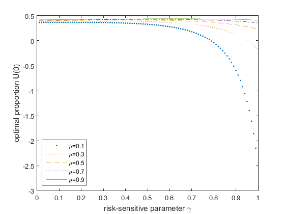
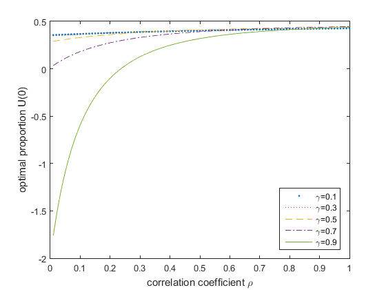
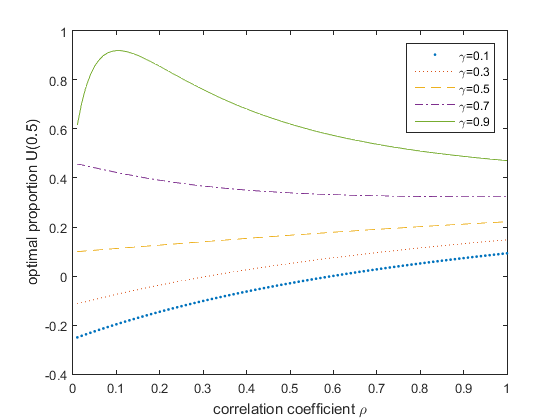
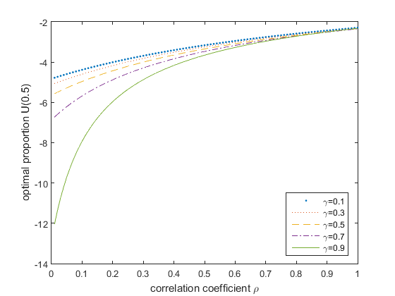
In Section 4, we use the new risk-sensitive stochastic maximum principle to solve the optimal investment problem in the financial market, as introduced in Section 2. We give the optimal investment strategy by virtue of the solution to one Riccati equation. The solvability of the Riccati equation is investigated under the risk-seeking case. In Section 5, by virtue of the numerical simulation, some figures are given to illustrate the optimal investment strategy and its sensitivity to the risk-sensitive parameter and the correlation coefficient respectively. Some concluding remarks are given in Section 6.
In this paper, we use to denote the Euclidean space of -dimensional vectors, to denote the space of matrices, and to denote the space of symmetric matrices. and are used to denote the scalar product and norm in the Euclidean space, respectively. A appearing in the superscript of a matrix, denotes its transpose. denote the first- and second-order partial derivatives with respect to for a differentiable function , respectively.
2 The Model and Problem Formulation
We consider a financial market, in which investors can choose two kinds of assets: one is risk-free and the other one is risky. The risk-free asset is called bond, whose price at time satisfies the ordinary differential equation (ODE):
|
|
|
(2.1) |
where is the constant interest rate. The risky asset is called stock, whose price at time is . Let satisfy the Ornstein-Uhlenbeck type process with correlated nosies:
|
|
|
(2.2) |
Here, the price of stock is influenced by two random noises: and , which are both one-dimensional Brownian motions under some probability measure on some given measurable space , and the correlation coefficient between these two Brown motions is a constant . That is, . The stock price volatility rates and are the nonzero constant, and is some coefficient. is linear in and is the deterministic log stock price trend. That means that , where and are constant.
Let be the amount of the investor’s wealth and is the proportion of the wealth invested in stock at time , so is the amount invested in the bond. In this paper, we require , which means no investment strategy constraints. The wealth dynamics of the investor with the initial state satisfy
|
|
|
(2.3) |
The investor hopes to maximize the expected utility (HARA case) in the terminal time :
|
|
|
(2.4) |
by choosing an optimal investment strategy , where is the risk-sensitive parameter. The is the expectation defined under the probability measure while is the expectation defined under another probability measure which will be introduced later.
Let us now explain the meaning of risk-sensitive by an intuitive argument. Define . Obviously, is differentiable at . Then Taylor’s expansion
yields
|
|
|
|
|
|
|
|
If is strictly concave near , then which is equivalent to . This will reduce the overall cost with a large which implies the investor is risk-seeking. Conversely, if is strictly convex near , then which is equivalent to . This will bring a penalty to the variance term in the overall cost. In this case, the investor tries to avoid a large deviation of from its mean , which implies the investor is risk-averse. Finally, if is close or equal to 0 which is equivalent to , then , in which case the risk-sensitive model
reduces to the risk-neutral one.
To solve the above problem, first we can rewrite the expectation in terms of an expected exponential-of-integral criterion. Applying Itô’s formula to , we can get
|
|
|
We eliminate the stochastic integral term by using the Girsanov transformation:
|
|
|
In order to make the change of probability measure argument valid (see Liptser and Shiryayev [35]), we assume that existing positive constants and satisfy the following inequality
|
|
|
(2.5) |
Then
|
|
|
(2.6) |
where and are Brownian motions under the probability measure with correlation coefficient still being , and
|
|
|
where
|
|
|
(2.7) |
Here is the state and is the control. We required is -adapted to the filtration and (2.5) holds. We call such an admissible control and denote by the admissible control set.
In order to simplify the problem, we replace by an equivalent state variable
|
|
|
(2.8) |
Then, by (2.6), we have
|
|
|
(2.9) |
So the expected HARA utility (2.4) is reduced to the expected exponential-of-integral form
|
|
|
(2.10) |
where is defined by (2.7). Hence we need to maximize (2.10) by choosing over .
In order to solve this problem, in the next section, we consider a general risk-sensitive stochastic control problem with two Brownian noises whose correlation coefficient is first. Then we apply the theoretic results to solve this problem in Section 5.
3 A General Risk-Sensitive Stochastic Control problem
In this section, we consider a general risk-sensitive stochastic control problem with correlated Brownian noises and give the necessary and sufficient conditions for the optimality.
Let the time duration . For any , we consider the following SDE:
|
|
|
(3.1) |
We will work in the weak formulation. For any , the class of admissible controls is the set of all six-tuple satisfying the following conditions.
1) is a complete probability space.
2) are both one-dimensional Brownian motions defined on with the correlation coefficient being , and is augmented by all the - set in .
3) is an adapted process on .
4) Under , for any , (3.1) admits a unique adapted solution on .
If there are no ambiguity, we will only write instead of the entire six-tuple . If is the unique solution to (3.1) associated with the input , we refer to as an admissible pair. In this paper, will denote the set of -valued, -adapted, square integrable processes on , and will denote the set of -valued, -adapted, essentially bounded processes on .
The cost functional associated with the initial condition and is given by
|
|
|
(3.2) |
where , the risk-sensitive parameter, is a given fixed constant. The risk-sensitive stochastic control problem associated with (3.1) and (3.2) is defined as follows:
|
|
|
(3.3) |
The value function associated with (7) is defined by
|
|
|
(3.4) |
Let we introduce the following assumptions:
(B1) The map , , where , and are measurable, and there exists a constant and a modulus of continuity such that for ,
|
|
|
Also and are uniformly bounded.
(B2) , are twice differentiable in , and there exists a modulus of continuity such that for ,
|
|
|
(B3)
(B4) is a convex subset of . The map are locally Lipschitz in , and their derivatives in are continuous in .
Let be an admissible pair for (3.3). We introduce the first- and second-order adjoint variables , , which are the solution to the following BSDEs, respectively:
|
|
|
(3.5) |
|
|
|
(3.6) |
where has the similar interpretations). And the Hamiltonian function is given by
|
|
|
|
(3.7) |
|
|
|
|
Though (3.5) is a nonlinear equation, it will be shown that our assumption are sufficient to guarantee the existence of unique solutions and to (3.5) and (3.6), respectively.
Theorem 3.1 (Risk-Sensitive Maximum Principle) Suppose that (B1)-(B3) hold. Let be an optimal pair for the risk-sensitive stochastic control problem (3.3). Then, there are unique solutions and to the first-order and the second-order adjoint equations (3.5) and (3.6) respectively, such that
|
|
|
(3.8) |
or equivalently,
|
|
|
(3.9) |
where we define -function as
|
|
|
(3.10) |
Sufficient conditions for optimality of the pair are as follows.
Theorem 3.2 (Sufficient Conditions for Optimality) Suppose that (B1)-(B4) hold. Let be an admissible pair, and , be the first- and second-order adjoint variables, respectively. Suppose is convex, is concave for all almost surely and (3.9) holds. Then is an optimal pair for problem (3.3).
Proof of the two theorems will be given in the Appendix.
4 Optimal Investment Problem: Explicit Solution in the Risk-Seeking Case
In this section, we will apply the results we got in the previous section and solve the problem in Section 2.
Let be an optimal pair. First of all, the first-order adjoint equation is as follows:
|
|
|
(4.1) |
Noting that in our state dynamics (2.9), the diffusion term is control independent, so the second-order adjoint variables disappear automatically and -function gets the form
|
|
|
(4.2) |
By the minimum condition (3.9), we obtain
|
|
|
(4.3) |
Given and substituting (4.3) into (2.9) and (4.1), gives the following forward-backward SDE (FBSDE):
|
|
|
(4.4) |
As in Yong and Zhou [36], we conjecture the solution to (4.4) is related by
|
|
|
(4.5) |
where and are some deterministic differentiable functions. Applying Itô’s formula to (4.5), it gives
|
|
|
(4.6) |
On the other hand, substituting (4.5) into (4.1), we get
|
|
|
(4.7) |
Equating the coefficients of (4.6) and (4.7), gives
|
|
|
(4.8) |
where is the solution rto the Riccati equation
|
|
|
(4.9) |
and is a solution to the following equation
|
|
|
(4.10) |
Then, by (4.3) and (4.5), we can get the optimal control in the following state feedback form:
|
|
|
(4.11) |
Next, we apply the approach in Shi [37] (see also Shi and Wu [5]), to give the analytical solution to the Riccati equation (4.9). For this target, we rewrite (4.9) as follows
|
|
|
(4.12) |
where we denote
|
|
|
(4.13) |
Assuming , that is,
|
|
|
(4.14) |
we can obtain
|
|
|
(4.15) |
where
|
|
|
(4.16) |
Using the denotation (4.13) we rewrite equation (4.10) as
|
|
|
(4.17) |
where
|
|
|
(4.18) |
The explicit solution to (4.17) is
|
|
|
(4.19) |
To summarize, we have the following result.
Theorem 4.1 Let (4.14) holds, then equations (4.9) and (4.10) admit unique solutions and , and the optimal control of our risk-sensitive stochastic control problem (2.9)-(2.10) has the feedback form (4.11).
Remark 4.1 Considering the case of , by (4.14), we obtain
|
|
|
(4.20) |
Obviously, compared with the risk-seeking investors in the most portfolio problem without relevant noise, the existence of correlated noise makes the upper bound larger. It is equivalent to expanding the risk to a certain extent, making some investors with low risk seeking become risk-averse.
In the case of , (4.20) can also be obtained from (4.14). Obviously, compared with the risk-seeking investors in the most portfolio problem without relevant noise, the existence of correlated noise makes the upper bound smaller. It is equivalent to reducing the risk to a certain extent, making some investors with risk-aversion become low risk seeking.
Remark 4.2 Due to (4.20), in this paper we could only obtain the explicit solution to our optimal investment problem in the risk-seeking case, since it relies on the solvability of the Riccati equation (4.9). However, as mentioned in the above remark, because of the introduction of the correlated coefficient , we could encounter some cases when the investors are risk-averse. Note this was impossible in Shi and Wu [5].
Appendix A Appendix
This appendix is devoted to prove Theorem 3.1 and Theorem 3.2. First, we consider the following stochastic control problem:
|
|
|
(A.1) |
Obviously, (3.3) reduces to the case of in (A.1). The value function is
|
|
|
(A.2) |
Note that , where is defined by (3.4). And (B3) implies that .
Suppose is an optimal triple. Assuming (B1), (B2), we can apply the similar technique of Peng [38] to (A.1) to obtain the following first- and second-order adjoint equations:
|
|
|
(A.3) |
|
|
|
(A.4) |
where the Hamiltonian is given by
|
|
|
(A.5) |
The adjoint equations (A.3) and (A.4) are linear BSDEs. Under (B1), (B2), for every admissible triple , there are unique solutions and to (A.3) and (A.4), respectively.
The -function for problem (A.1) associated with is defined by
|
|
|
(A.6) |
The maximum principle for (A.1) can be stated as follows.
Proposition A.1 Let (B1), (B2) hold. Let be an optimal triple for the problem (A.1). Then there are unique solutions and to (A.3) and (A.4), respectively, such that
|
|
|
(A.7) |
or equivalently,
|
|
|
(A.8) |
Sufficient conditions for the optimality of are as follows.
Proposition A.2 Let (B1), (B2), (B4) hold. Let be an admissible triple and satisfy (A.3) and (A.4). Suppose that is convex, is concave for all a.s., and (A.8) holds. Then is an optimal triple for (A.1).
In the following, we will transform the adjoint variables and in certain ways. Let be an optimal triple for (A.1), and
|
|
|
be associated with first-order adjoint variables satisfying (A.3), where , , and is the corresponding value function. Under (B3), .
We take the following transformation of the first-order adjoint variable:
|
|
|
(A.9) |
where .
Next, we will derive the equation for where is -valued and is scalar valued. First, notice that is the value function of problem (A.1) which has no running cost. Hence, it satisfies
|
|
|
(A.10) |
On the other hand, rearranging (A.9), we obtain . Applying Itô’s formula, and assuming that satisfies an equation of the following form:
|
|
|
(A.11) |
we obtain
|
|
|
(A.12) |
Noting that
|
|
|
(A.13) |
we obtain the following expression:
|
|
|
(A.14) |
Substituting the expression (A.3) for into (A.14), we can find that the diffusion terms of are
|
|
|
(A.15) |
|
|
|
(A.16) |
where , are -valued. Substituting (A.15), (A.16) back to (A.14) and using (A.3), it follows that the transformed first-order adjoint variable satisfied the following equation, where the terminal condition for is easily determined from (A.9):
|
|
|
(A.17) |
Expanding (A.17), it can be easily get
|
|
|
(A.18) |
and is a solution to (3.5). This explains how (3.5) is derived. Since our derivation can be reserved, it follows from the uniqueness property of (A.3) that this solution is unique.
Finally, since and , the last component of the extended first order adjoint is essentially the value function.
Now, let be the second-order adjoint variables satisfying (A.4). We propose the following transformation of the second-order adjoint variable:
|
|
|
(A.19) |
Assuming that
|
|
|
(A.20) |
for some processes , it follows from Itô’s formula and (A.19) that
|
|
|
(A.21) |
Substituting the expression for and notice (A.20), gives
|
|
|
(A.22) |
By (A.21), (A.19) and using Itô’s formula, we obtain
|
|
|
(A.23) |
where
|
|
|
(A.24) |
Reminding the definition of , we have
|
|
|
(A.25) |
Noticing that
|
|
|
(A.26) |
together with the transformation (A.15), (A.16), (A.19), (A.23), (A.24) and (A.25), we can obtain
|
|
|
Therefore, it follows that
|
|
|
where is the solution to (3.6). As in the first-order case, the solution is unique.
Now, we consider (3.8). By (A.9), (A.15), (A.16), (A.18), we have
|
|
|
(A.27) |
where is given by (3.7), and
|
|
|
Since , it follows that the maximum condition (A.7) is equivalent to
|
|
|
which gives us (3.8). The equivalent condition (3.9) can be get by direct manipulation. This complete the proofs of Theorems 3.1 and 3.2.


