Iterative Channel Estimation for
Discrete Denoising under Channel Uncertainty

Abstract

We propose a novel iterative channel estimation (ICE) algorithm that essentially removes the critical known noisy channel assumption for universal discrete denoising problem. Our algorithm is based on Neural DUDE (N-DUDE), a recently proposed neural network-based discrete denoiser, and it estimates the channel transition matrix as well as the neural network parameters in an alternating manner until convergence. While we do not make any probabilistic assumption on the underlying clean data, our ICE resembles Expectation-Maximization (EM) with variational approximation, and it takes advantage of the property that N-DUDE can always induce a marginal posterior distribution of the clean data. We carefully validate the channel estimation quality of ICE, and with extensive experiments on several radically different types of data, we show the ICE equipped neural network-based denoisers can perform universally well regardless of the uncertainties in both the channel and the clean source. Moreover, we show ICE becomes extremely robust to its hyperparameters, and show our denoisers with ICE significantly outperform the strong baseline that can handle the channel uncertainties for denoising, the widely used Baum-Welch (BW) algorithm for hidden Markov models (HMM).

1 Introduction

Denoising, which focuses on cleaning up noise-corrupted data, is one of the most studied topics in machine learning and signal processing. In particular, discrete denoising focuses on denoising the data that take finite-alphabet values. Such setting covers several applications in various domains, e.g., image denoising Ordentlich et al. (2003); Motta et al. (2011), DNA sequence denoising Laehnemann et al. (2016); Lee et al. (2017), and channel decoding Ordentlich et al. (2008), etc. Recently, utilizing quantized measurements from low-power sensors Romero et al. (2017) or DNA sequencing devices Goodwin et al. (2015) are getting more prevalent, thus, denoising such data is getting more important.

In Weissman et al. (2005), the universal setting for discrete denoising, in which no assumption on the underlying clean data was made, was first considerd. They devised a sliding-window algorithm called DUDE (Discrete Universal DEnoiser) with powerful theoretical guarantees and empirical performance. Despite the strong results, however, DUDE suffered from a couple of shortcomings; the performance of the algorithm deteriorates as the alphabet size grows and is quite sensitive to the choice of a hyperparameter, the window size $k$. In order to overcome such limitations, Moon et al. (2016) recently proposed Neural DUDE (N-DUDE), by introducing a neural network as an implicit context aggregator. It maintained the robustness with respect to both $k$ and the alphaset size, and as a result, N-DUDE achieved significantly better performance than DUDE. The main gist of N-DUDE was to devise “pseudo-labels” solely based on the noisy data, and train the neural network as a denoiser without any supervised training set with clean data.

Although both DUDE and N-DUDE did not make any assumptions on the underlying clean data, one critical assumption they both made is that the statistical characteristics of the noise mechanism is known to the denoiser. That is, the noise is modeled to be a Discrete Memoryless Channel (DMC), i.e., the index-independent noise, and the channel transition matrix was assumed to be completely known to the denoiser. While such assumption makes sense in some applications, e.g., when the noisy channel can be reliably estimated with known reference sequences, it can become a major weakness in competing with other methods that do not require such assumption. For example, the Baum-Welch (BW) algorithm Baum et al. (1970) combined with forward-backward (FB) recursion for hidden Markov models (HMM) Ephraim and Merhav (2002) can both estimate the channel (i.e., the emission probability) and the underlying clean data (i.e., the latent states) as long as the noisy observation can be modeled as an HMM.

In this paper, we aim to remove the known noise assumption of N-DUDE. Namely, the only assumption we make is that the noise mechanism is a DMC (like in HMM), but neither the channel transition matrix nor characteristics of the clean data (such as Markovity) are assumed to be known. Thus, our setting is a much more challenging one than that of Weissman et al. (2005); Moon et al. (2016) as we impose uncertainty on the noise model in addition to on the clean data. We propose a novel iterative channel estimation (ICE) algorithm such that learning the channel transition matrix and the neural network parameters can be done in an alternating manner that resembles Expectation-Maximization (EM). The key component of our algorithm is to approximate the “marginal posterior distribution” of the clean data, even though there might not exist one, with a posterior induced from the N-DUDE’s output distribution and carry out the variational approximation.

In our experimental results with various different types of data (e.g., images or DNA sequences), we show the effectiveness of our ICE by showing that denoising with the estimated channel achieves almost the identical denoising performance as with the true channel. We employ two neural network-based denoisers to evaluate the denoising performance with ICE; N-DUDE and CUDE (Context-aggregated Universal DEnoiser)(Ryu and Kim, 2018), in which the former is what ICE is based on, and the latter is another recently developed universal denoiser that is shown to outperform N-DUDE. Both algorithms that plug-in the estimated channel by ICE are shown to outperform the widely used BW with FB recursion, which models the noisy data as an HMM regardless of it being true. In addition, we show ICE is much more robust with respect to its hyperparameters and initializations compared to BW, which is sensitive to the initial transition and channel models. Finally, we give thorough experimental analyses on the channel estimation errors as well as the model approximation performance of ICE.

2 Notations and Related Work

To be self-contained, we introduce notations that mainly follow Moon et al. (2016). Throughout the paper, an $n$-tuple sequence is denoted as, e.g., $a^{n}=(a_{1},\ldots,a_{n})$, and $a_{i}^{j}$ refers to the subsequence $(a_{i},\ldots,a_{j})$. We denote the uppercase letters as random variables and the lowercase letters as either the realizations of the random variables or the individual symbols. We denote $\Delta^{d}$ as the probability simplex in $\mathbb{R}^{d}$. In the universal setting, the clean, underlying source data will be denoted as an individual sequence $x^{n}$ as we make no stochastic assumption on it. We assume each component $x_{i}$ takes a value in some finite set $\mathcal{X}$. For example, for binary data, $\mathcal{X}=\{0,1\}$, and for DNA data, $\mathcal{X}=\{\texttt{A},\texttt{C},\texttt{G},\texttt{T}\}$.

We assume $x^{n}$ is corrupted by a DMC, namely, the index-independent noise, and results in the noisy data, $Z^{n}$, of which each $Z_{i}$ takes a value in, again, a finite set $\mathcal{Z}$. The DMC is characterized by the channel transition matrix $\mathbf{\Pi}\in\mathbb{R}^{|\mathcal{X}|\times|\mathcal{Z}|}$, and the $(x,z)$-th element of $\mathbf{\Pi}$ stands for $\text{Pr}(Z=z|x)$. A natural assumption we make is that $\mathbf{\Pi}$ is of the full row rank. We also denote $\mathbf{\Pi}^{\dagger}=\mathbf{\Pi}^{\top}(\mathbf{\Pi}\mathbf{\Pi}^{\top})^{-1}$ as the Moore-Penrose pseudoinverse of $\mathbf{\Pi}$. Now, upon observing the entire noisy data $Z^{n}$, a discrete denoiser reconstructs the original data with $\hat{X}^{n}=(\hat{X}_{1}(Z^{n}),\ldots,\hat{X}_{n}(Z^{n}))$, where each reconstructed symbol $\hat{X}_{i}(Z^{n})$ takes its value in a finite set $\hat{\mathcal{X}}$. The goodness of the reconstruction is measured by the average denoising loss, $\frac{1}{n}\sum_{i=1}^{n}\mathbf{\Lambda}(x_{i},\hat{X}_{i}(Z^{n})),$ where the per-symbol loss $\mathbf{\Lambda}(x_{i},\hat{x}_{i})$ measures the loss incurred by estimating $x_{i}$ with $\hat{x}_{i}$. The loss is fully represented with a loss matrix $\mathbf{\Lambda}\in\mathbb{R}^{|\mathcal{X}|\times|\hat{\mathcal{X}}|}$.

The $k$-th order sliding window denoisers are the denoisers that are defined by a time-invariant mapping $s_{k}:\mathcal{Z}^{2k+1}\rightarrow\hat{\mathcal{X}}$. That is, $\hat{X}_{i}(Z^{n})=s_{k}(Z_{i-k}^{i+k})$. We also denote the tuple $(Z_{i-k}^{i-1},Z_{i+1}^{i+k})\triangleq\mathbf{C}_{i}$ as the $k$-th order double-sided context around the noisy symbol $Z_{i}$, and we let $\mathbf{C}[k]$ as the set of all such contexts. We also denote $\mathcal{S}\triangleq\{s:\mathcal{Z}\rightarrow\hat{\mathcal{X}}\}$ as the set of single-symbol denoisers that are sliding window denoisers with $k=0$. Note $|\mathcal{S}|=|\hat{\mathcal{X}}|^{|\mathcal{Z}|}$. Then, an alternative view of of $s_{k}(\cdot)$ is that $s_{k}(\mathbf{C}_{i},\cdot)\in\mathcal{S}$ is a single symbol denoiser defined by $\mathbf{C}_{i}$ and applied to $Z_{i}$.

When $\mathbf{\Pi}$ is known, as in (Moon et al., 2016, Section 3.1), we can devise an unbiased esimate of the true loss $\mathbf{\Lambda}$ as

$$\mathbf{L}=\mathbf{\Pi}^{\dagger}\bm{\rho}\in\mathbb{R}^{|\mathcal{Z}|\times|\mathcal{S}|},$$ (1)

in which $\bm{\rho}\in\mathbb{R}^{|\mathcal{X}|\times|\mathcal{S}|}$ with the $(x,s)$-th element is $\mathbb{E}_{Z|x}\mathbf{\Lambda}(x,s(Z))$, and $\mathbb{E}_{Z|x}(\cdot)$ stands for the expectation with respect to the distribution defined by the $x$-th row of $\mathbf{\Pi}$. Then, as shown in Moon et al. (2016); Weissman et al. (2007), $\mathbf{L}$ has the unbiased property, $\mathbb{E}_{Z|x}\mathbf{L}(Z,s)=\mathbb{E}_{Z|x}\mathbf{\Lambda}(x,s(Z))$.

2.1 Related work

DUDE Weissman et al. (2005) is a two-pass, sliding-window denoiser that has a linear complexity in data size $n$. For reconstruction at location $i$, DUDE takes $\mathbf{C}_{i}\in\mathbf{C}[k]$ and $Z_{i}\in\mathcal{Z}$, and applies the rule

$$\hat{X}_{i,\texttt{DUDE}}(\mathbf{C}_{i},Z_{i})=\arg\min_{\hat{x}\in\hat{\mathcal{X}}}\hat{\mathbf{p}}_{\text{emp}}(\cdot|\mathbf{C}_{i})^{\top}\mathbf{\Pi}^{\dagger}[\bm{\Lambda}_{\hat{x}}\odot\mathbf{\Pi}_{Z_{i}}],$$ (2)

in which $\hat{\mathbf{p}}_{\text{emp}}(\cdot|\mathbf{C}_{i})$ is an empirical probability vector on $Z_{i}$ given the context vector $\mathbf{C}_{i}$, obtained from the noisy data $Z^{n}$. That is, for a context $\mathbf{C}\in\mathbf{C}[k]$, the $z$-th element becomes

$$\hat{\mathbf{p}}_{\text{emp}}(z|\mathbf{C})=\frac{|\{j:\mathbf{C}_{j}=\mathbf{C},Z_{j}=z\}|}{|\{j:\mathbf{C}_{j}=\mathbf{C}\}|}.$$ (3)

Moreover, the $\bm{\Lambda}_{\hat{x}}$ and $\mathbf{\Pi}_{Z_{i}}$ in (2) stand for the $\hat{x}$-th and $Z_{i}$-th column of $\mathbf{\Lambda}$ and $\mathbf{\Pi}$, respectively. The rule (2) is based on the intuition from achieving the Bayes response using (3) and inverting the channel. For more rigorous details and results, we refer to the original paper Weissman et al. (2005).

Neural DUDE Moon et al. (2016) extends DUDE and defines a single neural network-based sliding-window denoiser, $\mathbf{p}^{k}(\mathbf{w},\cdot):\mathcal{Z}^{2k}\rightarrow\Delta^{|\mathcal{S}|}$, in which $\mathbf{w}$ stands for the parameters in the network. Following the alternative view on the sliding-window denoiser mentioned above, the network takes the context $\mathbf{C}_{i}$ and outputs a probability distribution on the single-symbol denoisers to apply to $Z_{i}$.

To train $\mathbf{w}$, N-DUDE defines the “pseudo-label” matrix $\mathbf{L}_{\text{new}}\in\mathbb{R}^{|\mathcal{Z}|\times|\mathcal{S}|}$ as

$$\mathbf{L}_{\text{new}}\triangleq-\mathbf{L}+L_{\text{max}}\mathbf{1}_{|\mathcal{Z}|}\mathbf{1}_{|\mathcal{S}|}^{\top},$$ (4)

in which $L_{\text{max}}\triangleq\max_{z,s}\mathbf{L}(z,s)$, and $\mathbf{1}_{|\mathcal{Z}|}$ and $\mathbf{1}_{|\mathcal{S}|}$ stand for the all-1 vectors with $|\mathcal{Z}|$ and $|\mathcal{S}|$ dimensions, respectively. By design, all the elements in $\mathbf{L}_{\text{new}}$ are non-negative and can be computed with $\mathbf{\Pi}$, $\mathbf{\Lambda}$, $z$ and $s$ (and not with the clean $x$). N-DUDE treats $\mathbf{L}_{\text{new}}^{\top}\mathds{1}_{Z_{i}}\in\mathbb{R}^{|\mathcal{S}|}$ as the target “pseudo-label” vector for the mapping to apply at location $i$ and minimizes the objective function,

$$\mathcal{L}(\mathbf{w},Z^{n},\mathbf{\Pi})\triangleq \frac{1}{n}\sum_{i=1}^{n}\mathcal{C}\Big{(}\mathbf{L}_{\text{new}}^{\top}\mathds{1}_{Z_{i}},\mathbf{p}^{k}(\mathbf{w},\mathbf{C}_{i})\Big{)}.$$ (5)

In (5), $\mathcal{C}(\mathbf{g},\mathbf{p})$ for $\mathbf{g}\in\mathbb{R}_{+}^{|\mathcal{S}|}$ and $\mathbf{p}\in\Delta^{|\mathcal{S}|}$ is the (unnormalized) cross-entropy, and $\mathds{1}_{Z_{i}}$ is the unit vector for the $Z_{i}$-th coordinate in $\mathbb{R}^{|\mathcal{Z}|}$. Note $\mathbf{L}_{\text{new}}^{\top}\mathds{1}_{Z_{i}}$ is not necessarily a one-hot vector, and from (1) and (4), the mapping $s$ with larger pseudo-label value should have smaller “true” loss in expectation.

Once (5) is minimized after sufficient number of iterations, the converged parameter is denoted as $\mathbf{w}^{\star}$. Then, the single-letter mapping defined by N-DUDE for the context $\mathbf{C}\in\mathbf{C}[k]$ is expressed as $s_{k,\texttt{N-DUDE}}(\mathbf{C},\cdot)=\arg\max_{s\in\mathcal{S}}\mathbf{p}^{k}(\mathbf{w}^{\star},\mathbf{C})_{s},$ and the reconstruction at location $i$ becomes

$$\hat{X}_{i,\text{N-DUDE}}(\mathbf{C}_{i},Z_{i})=s_{k,\text{N-DUDE}}(\mathbf{C}_{i},Z_{i}).$$ (6)

In summary, Neural DUDE denoises the noisy data after adaptively training the network parameters with the same noisy data. Moon et al. (2016) shows N-DUDE significantly outperforms DUDE, has more robustness with respect to $k$, and gets very close to the optimum denoising performance for stationary sources.

CUDE (Ryu and Kim, 2018) borrows the idea of using neural network from N-DUDE, but uses it differently to replace (3) in the DUDE rule with a neural network learned empirical distribution of $z$ given $\mathbf{C}$. Namely, it defines a network $\mathbf{p}_{\text{emp}}(\mathbf{w},\cdot):\mathcal{Z}^{2k}\rightarrow\Delta^{|\mathcal{Z}|}$ and train it by minimizing $\frac{1}{n}\sum_{i=1}^{n}\mathcal{C}(\mathds{1}_{Z_{i}},\mathbf{p}_{\text{emp}}(\mathbf{w},\mathbf{C}_{i})).$ Once the learned parameter $\mathbf{w}^{*}$ is obtained, CUDE plugs in $\mathbf{p}_{\text{emp}}(\mathbf{w}^{*},\mathbf{C}_{i}))$ in place of $\hat{\mathbf{p}}_{\text{emp}}(\cdot|\mathbf{C}_{i})$ in (2). (Ryu and Kim, 2018) shows CUDE outperforms N-DUDE primarily due to the reduced output size, $|\mathcal{Z}|$ vs. $|\mathcal{S}|$.

Baum-Welch (BW) algorithm Baum et al. (1970) for HMM   From the equations (2) and (5), we confirm that all of above three schemes require the exact knowledge on the channel $\mathbf{\Pi}$. As mentioned in Introduction, however, the Baum-Welch (BW) algorithm combined with forward-backward (FB) recursion for HMM is a powerful method that can denoise $Z^{n}$ without requiring such knowledge on the channel. Despite the strength and being widely used in practice Krogh et al. (1994); Huang et al. (1990), we note the BW based on HMM has some drawbacks, too. Firstly, the Markov assumption on the clean $x^{n}$ may not be accurate; i.e., $x^{n}$ may not have generated from a Markov source or the assumed order could have a mismatch from the true model. In such cases, the resulting BW and FB recursion based denoising will have poor performance. Secondly, the BW-based channel estimation may suffer from instability with respect to the initialization of the algorithm. In the later sections, we convincingly show that our proposed ICE can reliably estimate the channel, and the ICE combined N-DUDE and CUDE overcome the drawbacks of BW and achieve significant better denoising performance in realistic discrete data.

3 Iterative Channel Estimation for N-DUDE

Our ICE algorithm is based on N-DUDE, and Algorithm 1 summarizes its pseudo-code.

Algorithm 1 ICE algorithm for N-DUDE

0:  Noisy data $Z^{n}$, A N-DUDE model $\mathbf{p}^{k}(\mathbf{w},\cdot):\mathcal{Z}^{2k}\rightarrow\Delta^{|\mathcal{S}|}$

0:  Channel estimate $\hat{\mathbf{\Pi}}$, Network parameters $\hat{\mathbf{w}}$

  Randomly initialize $\mathbf{\Pi}^{(0)}$ and $\mathbf{w}^{(0)}$ and fix window size $k$. Set $t\leftarrow 0$

  while $|\mathcal{L}(\mathbf{w},Z^{n};\mathbf{\Pi}^{(t)})-\mathcal{L}(\mathbf{w},Z^{n};\mathbf{\Pi}^{(t-1)})|>10^{-3}$ do

     Compute $\mathbf{L}_{\text{new}}$ in (4) using $\mathbf{\Pi}^{(t)}$.

     Approximate E-step (update $\mathbf{w}$):  Obtain $\mathbf{w}^{(t+1)}$ and the induced posterior for each location $i$, $q(x_{i}|Z_{i-k}^{i+k};\mathbf{w}^{(t+1)})$, as following:

$$\mathbf{w}^{(t+1)} = \underset{\mathbf{w}}{\arg\min}\ \mathcal{L}(\mathbf{w},Z^{n};\mathbf{\Pi}^{(t)})$$ (7)

$$q(x_{i}|Z_{i-k}^{i+k};\mathbf{w}^{(t+1)}) \triangleq \sum_{s:s(Z_{i})=x_{i}}\mathbf{p}^{k}(\mathbf{w}^{(t+1)},\mathbf{C}_{i})_{s}$$ (8)

     M-step (update $\mathbf{\Pi}$): Obtain $\mathbf{\Pi}^{(t+1)}$ as

$$\mathbf{\Pi}^{(t+1)}(j,k)=\frac{\sum_{i=1}^{n}\mathds{1}_{\{Z_{i}=k\}}q(x_{i}=j|Z_{i-k}^{i+k};\mathbf{w}^{(t+1)})}{\sum_{i=1}^{n}q(x_{i}=j|Z_{i-k}^{i+k};\mathbf{w}^{(t+1)})}.$$ (9)

     $t\leftarrow t+1$

  end while

  $\hat{\mathbf{\Pi}}=\mathbf{\Pi}^{(t)}$. Do a final update (7) with $\hat{\mathbf{\Pi}},\mathbf{w}^{(t)}$ and obtain $\hat{\mathbf{w}}$

Remark: When carrying out the minimization in (7), we always do a warm-start from the weight of the previous iteration, $\mathbf{w}^{(t)}$, except for the first iteration. Moreover, (9) looks very similar to the M-step of BW, and the intuition behind these update formulae is given below.

3.1 Intuition behind ICE

The intuition behind the ICE algorithm lies in the argument of maximum likelihood estimation with variational approximation. That is, we maintain the stochastic setting of Weissman et al. (2005) and denote $p_{\mathcal{X}}(x^{n})$ as the (unknown) prior distribution of the clean sequence $x^{n}$. Then, we also denote $p(x^{n},Z^{n};\mathbf{\Pi}^{(t)})$ as the joint distribution of $(x^{n},Z^{n})$ induced from $p_{\mathcal{X}}(x^{n})$ and $\mathbf{\Pi}^{(t)}$, i.e., $p(x^{n},Z^{n};\mathbf{\Pi}^{(t)})=p_{\mathcal{X}}(x^{n})p(Z^{n}|x^{n};\mathbf{\Pi}^{(t)})=p_{\mathcal{X}}(x^{n})\prod_{i=1}^{n}\mathbf{\Pi}^{(t)}(x_{i},Z_{i}).$ Now, the standard variational lower bound on $\log p(Z^{n};\mathbf{\Pi}^{(t)})$ becomes

$$\sum_{x^{n}}Q(x^{n})\log\frac{p(x^{n},Z^{n};\mathbf{\Pi}^{(t)})}{Q(x^{n})}=\log p(Z^{n};\mathbf{\Pi}^{(t)})-D_{KL}\Big{(}Q(x^{n})\|p(x^{n}|Z^{n};\mathbf{\Pi}^{(t)})\Big{)}$$ (10)

in which $Q(x^{n})$ stands for any probability distribution on $x^{n}$, and $D_{KL}(\cdot\|\cdot)$ is the Kullback-Leibler divergence. For a fixed $\mathbf{\Pi}^{(t)}$, one can easily see that $Q(x^{n})$ that maximizes (10) becomes $Q(x^{n})=p(x^{n}|Z^{n};\mathbf{\Pi}^{(t)})$, the posterior of $x^{n}$ given $Z^{n}$ derived from the joint distribution $p(x^{n},Z^{n};\mathbf{\Pi}^{(t)})$. Note this is equivalent to the E-step in EM algorithm and BW for HMM, in particular. Given above $Q(x^{n})=p(x^{n}|Z^{n};\mathbf{\Pi}^{(t)})$, the standard M-step in BW solves

$$\underset{\mathbf{\Pi}}{\arg\max}\sum_{x^{n}}Q(x^{n})\log\frac{p(x^{n},Z^{n};\mathbf{\Pi})}{Q(x^{n})}$$ (11)

to obtain $\mathbf{\Pi}^{(t+1)}$, which results in using the marginal posterior $p(x_{i}|Z^{n};\mathbf{\Pi}^{(t)})$ in the update formula as in (9). Note in HMM, computing such marginal posterior can be done efficiently thanks to the Markov assumption on $x^{n}$. However, in our universal setting, in which no distributional assumption is made on $x^{n}$, obtaining the posterior $p(x^{n}|Z^{n};\mathbf{\Pi}^{(t)})$ or its marginal becomes intractable.

Therefore, instead of $Q(x^{n})=p(x^{n}|Z^{n};\mathbf{\Pi}^{(t)})$, our ICE uses

$$Q(x^{n})=\tilde{Q}(x^{n};\mathbf{\Pi}^{(t)})\triangleq\prod_{i=1}^{n}q(x_{i}|Z_{i-k}^{i+k};\mathbf{w}^{(t+1)})$$ (12)

as the approximate E-step expecting $D_{KL}(\tilde{Q}(x^{n};\mathbf{\Pi}^{(t)})\|p(x^{n}|Z^{n};\mathbf{\Pi}^{(t)}))$ becomes small such that the lower bound (10) becomes sufficiently tight. The reasoning for this approximation follows from the strong empirical performance of N-DUDE that suggests the induced posterior (8) becomes a good approximation for $p(x_{i}|Z^{n};\mathbf{\Pi}^{(t)}).$ Namely, note that with the true channel $\mathbf{\Pi}$, the optimum reconstruction for the $i$-th location for minimizing the average loss becomes

$$\hat{X}_{i,\text{opt}}(Z^{n})=\arg\min_{\hat{x}\in\hat{\mathcal{X}}}\sum_{x=1}^{|\mathcal{X}|}\mathbf{\Lambda}(x,\hat{x})p(x_{i}=x|Z^{n};\mathbf{\Pi}),$$ (13)

which depends on the marginal posterior, $p(x_{i}|Z^{n};\mathbf{\Pi})$. Now, as shown in (Moon et al., 2016, Figure 2), the reconstruction of N-DUDE, (6), which applies the mapping obtained by $\mathbf{p}^{k}(\mathbf{w}^{\star},\mathbf{C})$, can attain the optimum performance of (13) for sufficiently large $k$. Therefore, we can expect the induced posterior $q(x_{i}|Z_{i-k}^{i+k};\mathbf{w}^{\star})=\sum_{s:s(Z_{i})=x_{i}}\mathbf{p}^{k}(\mathbf{w}^{\star},\mathbf{C})_{s}$ approximates $p(x_{i}|Z^{n};\mathbf{\Pi})$ sufficiently well for large $k$. From above reasoning, our M-step, (9), follows from solving (11) with $Q(x^{n})$ given by the approximate E-step in (12), and the precise derivation is given in the Supplementary.

Remark: One important point to make is that it is not possible to devise an iterative channel estimation scheme like ICE based on CUDE Ryu and Kim (2018). The reason is because in CUDE, the channel $\mathbf{\Pi}$ only occurs in the final denoising rule (2), and learning the neural network has nothing to do with $\mathbf{\Pi}$. In N-DUDE, however, $\mathbf{\Pi}$ is used to compute the pseudo-labels (4) for training the network, hence, an updated channel would lead to an updated network. Moreover, from the updated network, N-DUDE can naturally induce the marginal posterior (8) to carry out the M-step to update $\mathbf{\Pi}$.

4 Experimental Results

Data and training details  We carry out extensive experiments using synthetic data, real binary images, and Oxford nanopore MinION DNA sequence data to show the effectiveness and robustness of our ICE algorithm. All the experiments were done with Python 3.6 and Keras with Tensorflow backend. For the approximate E-step in (7), we used the Adam optimizer Kingma and Ba (2015) with default setting to minimize the objective function. The number of epochs for each iteration was set to 10 for synthetic and real binary image data and 20 for DNA data. The initial learning rate for the first iteration was $10^{-3}$, then from the second iteration, we used $10^{-4}$. As shown below in Figure 3, the objective function quickly converges after a few iterations, hence, we stopped the estimation process after the third iteration in all of our experiments. For the network architectures, we used 3 fully connected layers with 40 nodes and 160 nodes for synthetic/binary image data and DNA data, respectively.

4.1 Synthetic data

First, we carry out the experiment on synthetic data to validate the performance of ICE. Following Moon et al. (2016), we generated the clean binary data from a binary symmetric Markov chain (BSMC) with transition probability $\alpha=0.1$. The data was corrupted by a binary symmetric channel (BSC) $\mathbf{\Pi}$ with cross-over probability $\delta=0.3$ to result in the noisy sequence $Z^{n}$, which becomes a hidden Markov process. The length of the sequence was set to $n=10^{6}$, and the Hamming loss was used to set the Bit Error Rate (BER) as $\frac{1}{n}\sum_{i=1}^{n}\mathds{1}\{x_{i}\neq\hat{x}_{i}\}$. We report the normalized error, obtained by dividing BER with $\delta$. The denoising results on this data are given in the left and center plots of Figure 1, in which the left shows with respect to the window size $k$ and the center shows with respect to the initially assumed $\mathbf{\Pi}^{(0)}$. Note since $Z^{n}$ is a hidden Markov process in this case, the FB-Recursion that knows $\mathbf{\Pi}$ and the state transition probability $\alpha$ can achieve the optimum denoising performance, shown as purple lines (i.e., lower bounds) in the figures.

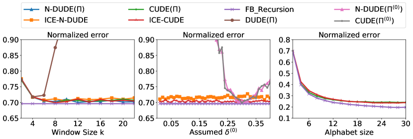
Figure 1: Denosing results for HMM with respect to window size $k$ (left), assumed $\delta^{(0)}$ (center), and the alphabet size $|\mathcal{X}|$ (right). The vertical axes for three figures correspond to the normalized error rates.

In Figure 1 (left), DUDE($\mathbf{\Pi}$), N-DUDE($\mathbf{\Pi}$) and CUDE($\mathbf{\Pi}$) stand for the results of the three schemes that exactly know the true channel $\mathbf{\Pi}$. We can confirm the universality of those methods since they almost achieve the optimum performance, while not knowing the source is a Markov. Also, N-DUDE($\mathbf{\Pi}$) and CUDE($\mathbf{\Pi}$) are much more robust with respect to $k$ than DUDE($\mathbf{\Pi}$). For our ICE, we initialized $\mathbf{\Pi}^{(0)}$ as BSC with crossover probablility $\delta^{(0)}=0.1$, and we observe ICE-N-DUDE and ICE-CUDE, which plug-in the estimated channel by ICE to N-DUDE and CUDE, respectively, work very well and essentially achieve the same performances as their counterparts that know $\mathbf{\Pi}$. We stress that this is a nontrivial result since ICE just observes $Z^{n}$ and provides an accurate enough estimation of $\mathbf{\Pi}$ to achieve the optimum performance, only with the independent noise assumption.

In Figure 1 (center), we show the robustness of ICE with respect to varying initially assumed $\delta^{(0)}$, while fixing the window size $k=16$. In the figure, N-DUDE($\mathbf{\Pi}^{(0)}$) and CUDE($\mathbf{\Pi}^{(0)}$) are the schemes that run with $\mathbf{\Pi}^{(0)}$, which can be potentially mismatched with the true $\mathbf{\Pi}$, and we clearly see they become very sensitive to the mismatch of the assumed $\mathbf{\Pi}^{(0)}$. In contrast, ICE becomes extremely robust to the initial $\mathbf{\Pi}^{(0)}$ such that both ICE-N-DUDE and ICE-CUDE almost achieve the optimum performance regardless of the initially assumed $\delta^{(0)}$.

In Figure 1 (right), we also investigate the performance of ICE with respect to the alphabet size of data. We increased the alphabet size of the Markove source, $|\mathcal{X}|$ (and $|\mathcal{Z}|$), from 2 to 30, and for each case, the transition probabilities from a state to others were set to be uniform as $0.1/(|\mathcal{X}|-1)$. $n$ was $5\times 10^{6}$, and the true $\mathbf{\Pi}$ was set such that $\mathbf{\Pi}(i,i)=0.7$ and $\mathbf{\Pi}(i,j)=0.3/(|\mathcal{Z}|-1)$ for $i\neq j$. The initial $\mathbf{\Pi}^{(0)}$ for ICE was set such that $\mathbf{\Pi}^{(0)}(i,i)=0.9$ and $\mathbf{\Pi}^{(0)}(i,j)=0.1/(|\mathcal{Z}|-1)$ for $i\neq j$. We compared CUDE($\mathbf{\Pi}$), ICE-CUDE and FB-Recursion, and again, ICE-CUDE performs almost as well as CUDE($\mathbf{\Pi}$), robustly over the alphabet sizes. The gap from FB-Recursion is primarily due to the fixed $n$, and we beleive it will close once $n$ grows with the alphabet size.

4.2 Binary image

Now, we move on to the experiments using more realistic binary images as clean data. We tested on two datasets: PASCAL and Standard. PASCAL consists of 50 binarized grayscale images that we obtained from PASCAL VOC 2012 dataset Everingham et al. , and Standard consists of 8 binarized standard images that are widely used in image processing, {Barbara, Boat, C.man, Couple, Einstein, fruit, Lena, Peppers}. We tested with three noise levels and applied non-symmetric channels with average noise levels of $0.1$, $0.2$, and $0.3$, and the exact $\mathbf{\Pi}$’s are given in the Supplementary Material. As in Moon et al. (2016), we raster scanned the images and converted them to 1-D sequences.

In Table 1, we compare the normalized errors of ICE-N-DUDE and ICE-CUDE with BW that assume the images are Markov. BW_1st, BW_2nd, and BW_3rd correspond to BW with various Markov order assumptions. N-DUDE($\mathbf{\Pi}$) and CUDE($\mathbf{\Pi}$), which are known to achieve the state-of-the-art for binary image denoising with known channel, are shown as lower bounds. We fixed the window size to $k=50$ for all neural network based schemes. For both ICE and BW, we set the initial $\mathbf{\Pi}^{(0)}$ as BSC with $\delta^{(0)}=0.1$ for all noise levels. For the exact procedure of running ICE and training denoisers with multiple images, we refer to the Supplementary Material.

Table 1: Denoising results for real binary images.

Noise level	$\delta=0.1$		$\delta=0.2$		$\delta=0.3$
Methods \Dataset	PASCAL	Standard	PASCAL	Standard	PASCAL	Standard
BW_1st	0.4294	0.5469	0.3508	0.4726	0.5088	0.5716
BW_2nd	0.4770	0.6342	0.4025	0.5149	0.3829	0.5020
BW_3rd	0.5996	1.0943	0.5619	0.7523	0.5277	0.7415
ICE-N-DUDE	0.3516	0.4120	0.3223	0.3771	0.3429	0.4286
ICE-CUDE	0.3512	0.4038	0.3205	0.3712	0.3438	0.4266
N-DUDE ($\mathbf{\Pi}$)	0.3540	0.3981	0.3300	0.3826	0.3494	0.4524
CUDE ($\mathbf{\Pi}$)	0.3259	0.3748	0.3171	0.3684	0.3396	0.4245

In the table, we see that both ICE-N-DUDE and ICE-CUDE significantly outperform all three BW methods for all noise levels and datasets, and they get very close to N-DUDE($\mathbf{\Pi}$) and CUDE($\mathbf{\Pi}$), respectively. We also confirm the superiority of CUDE over N-DUDE, as claimed in Ryu and Kim (2018). Moreover, note the BW schemes become sensitive depending the noise level and dataset; i.e., for $\delta=0.1,0.2$, BW_1st performs the best, while for $\delta=0.3$, BW_2nd is superior. Such difficulty of accurately determining the best order of HMM for a given dataset is one of the main drawbacks of BW method. On the contrary, ICE-N-DUDE and ICE-CUDE work universally well for all sources and noise levels, and neither the clean source modeling nor the true channel $\mathbf{\Pi}$ was necessary.

4.3 DNA sequence

We now apply ICE to DNA sequence denoising and mainly follow the experimental setting of (Moon et al., 2016, Section 5.3); namely, we obtained 16S rDNA reference sequences for 20 species and randomly generated noiseless template reads $x^{n}$ of length $n=2,469,111$. Then, we used the same $\mathbf{\Pi}$ in Moon et al. (2016), which had $20.375\%$ average error rate, to corrupt $x^{n}$ and obtain $Z^{n}$. The true (asymmetric) $\mathbf{\Pi}$ is given in the Supplementary Material. For ICE, the initial $\mathbf{\Pi}^{(0)}$ was assumed to be $\mathbf{\Pi}^{(0)}(i,i)=0.6$ and $\mathbf{\Pi}^{(0)}(i,j)=0.4/(|\mathcal{Z}|-1)$ for $i\neq j$. We also abuse the notation and define $\delta^{(0)}\triangleq\sum_{j\neq i}\mathbf{\Pi}^{(0)}(i,j)$ which becomes $0.4$ for all $i$. Note as shown in (Lee et al., 2017; Moon et al., 2016), DUDE($\mathbf{\Pi}$) and N-DUDE($\mathbf{\Pi}$) can achieve the state-of-the-art for DNA sequence denoising as well.

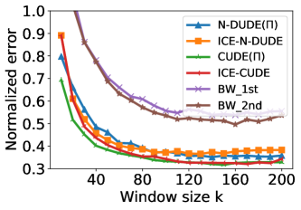
(a) Error rate with respect to window size k

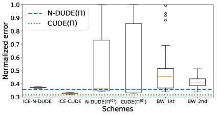
(b) Boxplots of error rates with varying initial $\delta^{(0)}$.

Figure 2: Denosing results for real DNA data with respect to window size $k$ & initial $\mathbf{\Pi}^{(0)}$.

Figure 2(a) shows the denoising results with varying window size $k$, and Figure 2(b) shows the boxplots of normalized errors with window size $k=150$ and varying initial $\delta^{(0)}$’s within the range $0.01\sim 0.40$ (40 samples). BW_1st and BW_2nd completely failed for this experiment, resulting in the normalized error rate of $1.440$ and $3.153$, respectively. Thus, we could not include them in the figure, and we instead included the results of a hybrid method, i.e, running N-DUDE with BW estimated channels. BW_1st and BW_2nd in the figure stand for such hybird of BW with N-DUDE.

Paralleling the results in the previous sections, we observe from Figure 2(a) that ICE-N-DUDE and ICE-CUDE get very close to N-DUDE($\mathbf{\Pi}$) and CUDE($\mathbf{\Pi}$), respectively, and significantly outperform the BW hybrid methods, as $k$ increases. This shows the accuracy and effectiveness of ICE; its channel estimation quality is much better than BW when the underlying $x^{n}$ is far from being a Markov and while it is based on N-DUDE, the estimated channel can be readily plugged-in to other scheme like CUDE. We believe this is quite a strong result, since ICE-CUDE can remove almost 70% of noise solely based on $Z^{n}$ and with no other information on the noise and the clean source. Moreover, in Figure 2(b), we see that ICE-N-DUDE and ICE-CUDE are extremely robust with respect to the initial $\delta^{(0)}$, while the mismatched N-DUDE($\mathbf{\Pi}^{(0)}$) and CUDE($\mathbf{\Pi}^{(0)}$) completely fails for wrong initializations. Moreover the BW hybrid methods also show large variance, mainly due to the sensitivity of the channel estimation quality of BW with respect to the initially assumed $\delta^{(0)}$.

4.4 Convergence & estimation analyses

We now give a closer analyses on the channel estimation performance of ICE for all of our experiments given in above sections. Figure 3 shows the following two metrics; (a) $|\mathcal{L}(\mathbf{w}^{\star},Z^{n};\mathbf{\Pi})-\mathcal{L}(\mathbf{w}^{(t)},Z^{n};\mathbf{\Pi})|$ and (b) $\|\mathbf{\Pi}-\mathbf{\Pi}^{(t)}\|_{1}/|\mathcal{X}||\mathcal{Z}|$. The first metric shows the difference between the value of the objective function (5) for N-DUDE($\mathbf{\Pi}$) parameter $\mathbf{w}^{\star}$ and for the model $\mathbf{w}^{(t)}$ after each approximate E-step of ICE. Note (5) is computed with the true $\mathbf{\Pi}$. The second metric is the normalized $L_{1}$-norm of $\mathbf{\Pi}-\mathbf{\Pi}^{(t)}$, which directly measures the channel estimation accuracy.

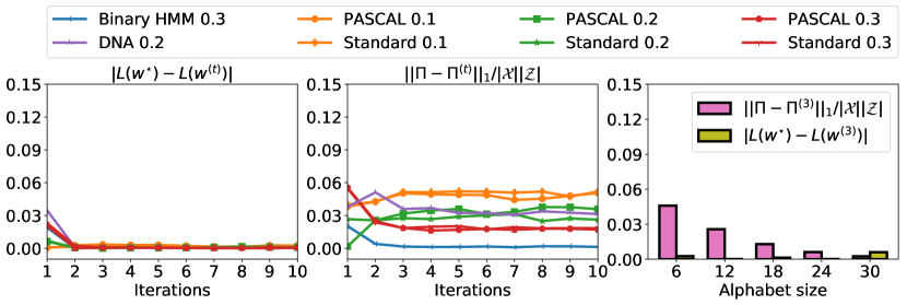
Figure 3: Convergence and estimation performance analysis

The first two figures show the two metrics for all experiments, respectively, except for the large alphabet Markov source case, with respect to the iteration $t$ of ICE. For metric (a), we observe that the difference becomes very small after just a few iterations for all cases. The result suggests that $\mathbf{w}^{(t)}$ of ICE and $\mathbf{w}^{\star}$ become indistinguishable from the perspective of objective function value, hence, it justifies the good performance of ICE-N-DUDE in denoising experiments. For metric (b), we observe the estimation errors also become small and stable with respect to the iteration $t$. The excellent denoising performance of ICE-CUDE, which just plugs-in the estimated channel to CUDE, confirms that such level of error is tolerable and has negligible effect in denoising. Moreover, the estimation errors seem to get smaller for larger noise levels. The third figure shows the two metrics at iteration 3 for the large alphabet Markov source case in Section 4.1. Again, they both become extremely small confirming the decent estimation quality of ICE for large alphabet case.

5 Conclusion

In this paper, we proposed a novel iterative channel estimation method for removing the known channel assumption of N-DUDE. The resulting ICE-N-DUDE and ICE-CUDE achieved excellent denoising performance for various different types of data, without any knowledge on the channel and the clean source. For future work, we plan to extend this approach to more general settings, e.g., to general state estimation beyond denoising and to continuous-alphabet case.

6 Derivation of the M-step of ICE

Consider the maximization problem of (Eq.(11), Manuscript) using $Q(x^{n})$ as in (Eq.(12), Manuscript) to obtain the updated $\mathbf{\Pi}^{(t+1)}$ from $\mathbf{\Pi}^{(t)}$.

$$\mathbf{\Pi}^{(t+1)}= \underset{\mathbf{\Pi^{(t)}}}{\arg\max}\sum_{x^{n}}\tilde{Q}(x^{n};\mathbf{\Pi}^{(t)})\log\frac{p(x^{n},Z^{n};\mathbf{\Pi}^{(t)})}{\tilde{Q}(x^{n};\mathbf{\Pi}^{(t)})}$$

$$= \underset{\mathbf{\Pi^{(t)}}}{\arg\max}\sum_{x^{n}}\tilde{Q}(x^{n};\mathbf{\Pi}^{(t)})\log p(x^{n},Z^{n};\mathbf{\Pi}^{(t)})$$

$$= \underset{\mathbf{\Pi^{(t)}}}{\arg\max}\sum_{x^{n}}\tilde{Q}(x^{n};\mathbf{\Pi}^{(t)})\log p_{\mathcal{X}}(x^{n})p(Z^{n}|x^{n};\mathbf{\Pi}^{(t)})$$

$$= \underset{\mathbf{\Pi^{(t)}}}{\arg\max}\sum_{x^{n}}\tilde{Q}(x^{n};\mathbf{\Pi}^{(t)})\log\prod_{i=1}^{n}\mathbf{\Pi}^{(t)}(x_{i},Z_{i})$$

$$= \underset{\mathbf{\Pi^{(t)}}}{\arg\max}\sum_{x^{n}}\tilde{Q}(x^{n};\mathbf{\Pi}^{(t)})\sum_{i=1}^{n}\sum_{j=1}^{|\mathcal{X}|}\sum_{k=1}^{|\mathcal{Z}|}\mathds{1}_{\{x_{i}=j,Z_{i}=k\}}\log\mathbf{\Pi}^{(t)}(j,k)$$ (14)

Since above maximization process has following constraint, $\sum_{k=1}^{|\mathcal{Z}|}\mathbf{\Pi}^{(t)}_{jk}=1$, we can consider Lagrangian of (14)

$$L(\mathbf{\Pi}^{(t)},\bm{\lambda})= \sum_{x^{n}}\tilde{Q}(x^{n};\mathbf{\Pi}^{(t)})\sum_{i=1}^{n}\sum_{j=1}^{|\mathcal{X}|}\sum_{k=1}^{|\mathcal{Z}|}\mathds{1}_{\{x_{i}=j,Z_{i}=k\}}\log\mathbf{\Pi}^{(t)}(j,k)+\sum_{j=1}^{|\mathcal{X}|}\bm{\lambda}_{j}(1-\sum_{k=1}^{|\mathcal{Z}|}\mathbf{\Pi}^{(t)}(j,k))$$ (15)

Then, to apply the KKT conditon, the partial derivatives of the Lagrangian w.r.t $\mathbf{\Pi}^{(t)}(j,k)$ and $\bm{\lambda}_{j}$ becomes

$$\frac{\partial L}{\partial\mathbf{\Pi}^{(t)}(j,k)}= \frac{1}{\mathbf{\Pi}^{(t)}(j,k)}\sum_{x^{n}}\tilde{Q}(x^{n};\mathbf{\Pi}^{(t)})\sum_{i=1}^{n}\mathds{1}_{\{x_{i}=j,Z_{i}=k\}}-\bm{\lambda}_{j}$$

$$\frac{\partial L}{\partial\bm{\lambda}_{j}}= 1-\sum_{k=1}^{|\mathcal{Z}|}\mathbf{\Pi}^{(t)}_{jk}.$$ (16)

Now, assume that the parameter satisfying KKT condition is $\mathbf{\Pi}^{(t+1)}$. Then,

$$\mathbf{\Pi}^{(t+1)}(j,k)=\frac{1}{\bm{\lambda}_{j}}\sum_{x^{n}}\tilde{Q}(x^{n};\mathbf{\Pi}^{(t)})\sum_{i=1}^{n}\mathds{1}_{\{x_{i}=j,Z_{i}=k\}}$$ (17)

Using (16) and (17),

$$\bm{\lambda}_{j}= \sum_{x^{n}}\tilde{Q}(x^{n};\mathbf{\Pi}^{(t)})\sum_{i=1}^{n}\mathds{1}_{\{x_{i}=j\}}$$

$$\therefore\mathbf{\Pi}^{(t+1)}(j,k)= \frac{\sum_{x^{n}}\tilde{Q}(x^{n};\mathbf{\Pi}^{(t)})\sum_{i=1}^{n}\mathds{1}_{\{x_{i}=j,Z_{i}=k\}}}{\sum_{x^{n}}\tilde{Q}(x^{n};\mathbf{\Pi}^{(t)})\sum_{i=1}^{n}\mathds{1}_{\{x_{i}=j\}}}$$ (18)

However, we can change (18) to an expression that contains (Eq.(12), Manuscript).

$$\sum_{x^{n}}\tilde{Q}(x^{n};\mathbf{\Pi}^{(t)})\sum_{i=1}^{n}\mathds{1}_{\{x_{i}=j,Z_{i}=k\}}= \sum_{i=1}^{n}\sum_{x^{n}}\mathds{1}_{\{x_{i}=j,Z_{i}=k\}}\tilde{Q}(x^{n};\mathbf{\Pi}^{(t)})$$

$$= \sum_{i=1}^{n}\sum_{x^{n}}\mathds{1}_{\{x_{i}=j,Z_{i}=k\}}\prod_{l=1}^{n}q(x_{l}|Z_{l-k}^{l+k};\mathbf{w}^{(t+1)})$$

$$= \sum_{i=1}^{n}\sum_{x_{i}}\mathds{1}_{\{x_{i}=j,Z_{i}=k\}}q(x_{i}|Z_{i-k}^{i+k};\mathbf{w}^{(t+1)})$$

$$= \sum_{i=1}^{n}\mathds{1}_{\{Z_{i}=k\}}q(x_{i}=j|Z_{i-k}^{i+k};\mathbf{w}^{(t+1)})$$

Likewise,

$$\sum_{x^{n}}\tilde{Q}(x^{n};\mathbf{\Pi}^{(t)})\sum_{i=1}^{n}\mathds{1}_{\{x_{i}=j\}}=\sum_{i=1}^{n}q(x_{i}=j|Z_{i-k}^{i+k};\mathbf{w}^{(t+1)})$$

$$\therefore\mathbf{\Pi}^{(t+1)}(j,k)=\frac{\sum_{i=1}^{n}\mathds{1}_{\{Z_{i}=k\}}q(x_{i}=j|Z_{i-k}^{i+k};\mathbf{w}^{(t+1)})}{\sum_{i=1}^{n}q(x_{i}=j|Z_{i-k}^{i+k};\mathbf{w}^{(t+1)})}$$

7 Experimental Details

7.1 Output dimension reduction

As a separate contribution, we also address one additional limitation of N-DUDE. Namely, the original N-DUDE has output size of $|\mathcal{S}|=|\mathcal{Z}|^{|\hat{\mathcal{X}}|}$, which can quickly grow very large when the alphabet size of the data grows. For example, even for DNA sequence that has alphabet size of 4, the output size of $\mathbf{p}^{k}(\mathbf{w},\cdot)$ becomes $|\mathcal{S}|=4^{4}=256$ as shown in Figure 4. Such exponential growth of the output size may cause overfitting and inaccurate approximation for the induced posterioir (Eq.(8), Manuscript).

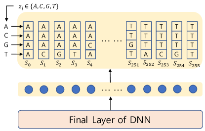
Figure 4: The original output layer of N-DUDE for DNA data.

In order to make ICE-N-DUDE more scalable with large alphabet size, we considered two output dimension reduction methods as shown in Figure 5, shown with the DNA example. First, Figure 5(a) shows reducing the output size to $|\hat{\mathcal{X}}||\mathcal{Z}|=16$ by implementing $|\mathcal{Z}|$ different output layers having $|\mathcal{X}|$ outputs. Note all 256 mappings in Figure 4 can be enumerated by combining the partial mappings for each $Z_{i}$ given in Figure 5(a). Second, Figure 5(b) shows further reducing the output size to $|\hat{\mathcal{X}}|+1=5$. That is, by simplifying the denoising to either “saying-what-you-see” (i.e., $s(Z_{i})=Z_{i}$) or “saying-one-in-$\hat{\mathcal{X}}$, we can work with this reduced output size. With this reduction, the unnecessary variance in the model could reduce and the summation in (Eq.(8), Manuscript) would always involve only two mappings, hence, the approximation quality of $D_{KL}(\tilde{Q}(x^{n};\mathbf{\Pi}^{(t)})\|p(x^{n}|Z^{n};\mathbf{\Pi}^{(t)}))$ could improve. In fact, in our experimental results, we observed the second reduction yields much better denoising as well as the channel estimation results, hence, all of our results regarding N-DUDE employ the second reduction structure.

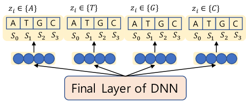
(a) 16 mappings

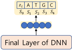
(b) 5 mappings

Figure 5: The reduced output layer of N-DUDE for DNA data.

7.2 Training details for binary image denoising

In the binary image denoising experiment (Section 4.2), we used the first 10 images in PASCAL and all 8 images for Standard for estimating the channel before carrying out the denoising in each set. For ICE-N-DUDE and ICE-CUDE, the estimated channel by ICE was plugged-in, and the network parameters were fine-tuned for each image separately. For fair comparison, N-DUDE($\mathbf{\Pi}$) and CUDE($\mathbf{\Pi}$) were also first trained with the same images as ICE and BW, before fine-tuning for each image.

7.3 True channels

We used three different asymmetric $\mathbf{\Pi}$’s in binary image denoising experiments with each $\mathbf{\Pi}$ having average noise level of 0.1, 0.2 and 0.3.

$$\mathbf{\Pi}_{0.1}=\begin{bmatrix}0.88&0.12\\ 0.09&0.91\end{bmatrix}$$

$$\mathbf{\Pi}_{0.2}=\begin{bmatrix}0.83&0.17\\ 0.23&0.77\end{bmatrix}$$

$$\mathbf{\Pi}_{0.3}=\begin{bmatrix}0.72&0.28\\ 0.33&0.67\end{bmatrix}$$

For the DNA experiment, we used $4\times 4$ asymmetric $\mathbf{\Pi}$ as below.

$$\mathbf{\Pi}_{DNA}=\begin{bmatrix}0.8122&0.0034&0.0894&0.0950\\ 0.0096&0.8237&0.0808&0.0859\\ 0.1066&0.0436&0.7774&0.0724\\ 0.0704&0.0690&0.0889&0.7717\\ \end{bmatrix}$$

References

- Baum et al. [1970] L. Baum, T. Petrie, G. Soules, and N. Weiss. A maximization technique occuring in the statistical analysis of probabilistic functions of Markov chains. Annals of Mathematical Statistics, 41(164-171), 1970.
- Ephraim and Merhav [2002] Y. Ephraim and N. Merhav. Hidden markov processes. IEEE Trans. Inform. Theory, 48(6):1518–1569, 2002.
-
[3]
M. Everingham, L. Van Gool, C. K. I. Williams, J. Winn, and A. Zisserman.
The PASCAL Visual Object Classes Challenge 2012 (VOC2012)
Results.
http://www.pascal-network.org/challen
ges/VOC/voc2012/workshop/index.html. - Gemelos et al. [2006a] G. Gemelos, S. Sigurjonsson, and T. Weissman. Algorithms for discrete denoising under channel uncertainty. IEEE Trans. Signal Process., 54(6):2263–2276, 2006a.
- Gemelos et al. [2006b] G. Gemelos, S. Sigurjonsson, and T. Weissman. Universal minimax discrete denoising under channel uncertainty. IEEE Trans. Inform. Theory, 52:3476–3497, 2006b.
- Goodwin et al. [2015] S. Goodwin, J. Gurtowski, S. Ethe-Sayers, P. Deshpande, M. Schatz, and W. McCombie. Oxford Nanopore sequencing, hybrid error correction, and de novo assembly of a eukaryotic genome. Genome Res., 2015.
- Huang et al. [1990] X. Huang, Y. Ariki, and M. Jack. Hidden Markov Models for Speech Recognition. Edinburgh University Press, Edinburgh, 1990.
- Kingma and Ba [2015] D. Kingma and J. Ba. Adam: A method for stochastic optimization. In International Conference on Learning Representations (ICLR), 2015.
- Krogh et al. [1994] A. Krogh, M. Brown, I. S. Mian, K. Sjölander, and D. Haussler. Hidden Markov models in computational biology: Applications to protein modeling. Journal of Molecular Biology, 235:1501–1531, Feb. 1994.
- Laehnemann et al. [2016] D. Laehnemann, A. Borkhardt, and A. McHardy. Denoising DNA deep sequencing data– high-throughput sequencing errors and their corrections. Brief Bioinform, 17(1):154–179, 2016.
- Lee et al. [2017] B. Lee, T. Moon, S. Yoon, and T. Weissman. DUDE-Seq: Fast, flexible, and robust denoising for targeted amplicon sequencing. PLoS ONE, 12(7):e0181463, 2017.
- Moon et al. [2016] T. Moon, S. Min, B. Lee, and S. Yoon. Neural universal discrete denosier. In Neural Information Processing Systems (NIPS), 2016.
- Motta et al. [2011] G. Motta, E. Ordentlich, I. Ramirez, G. Seroussi, and M. J. Weinberger. The iDUDE framework for grayscale image denoising. IEEE Trans. Image Processing, 20:1–21, 2011.
- Ordentlich et al. [2003] E. Ordentlich, G. Seroussi, S. Verdú, M. Weinberger, and T. Weissman. A universal discrete image denoiser and its application to binary images. In IEEE ICIP, 2003.
- Ordentlich et al. [2008] E. Ordentlich, G. Seroussi, S. Verdú, and K. Viswanathan. Universal algorithms for channel decoding of uncompressed sources. IEEE Trans. Inform. Theory, 54(5):2243–2262, 2008.
- Romero et al. [2017] D. Romero, S.-J. Kim, G. B. Giannakis, and R. Lopez-Valcarce. Learning power spectrum maps from quantized power measurements. IEEE Trans. Signal Process., 2547 - 2560, 2017.
- Ryu and Kim [2018] J. Ryu and Y.-H. Kim. Conditional distribution learning with neural networks and its application to universal image denoising. pages 3214–3218, 10 2018. doi: 10.1109/ICIP.2018.8451573.
- Weissman et al. [2005] T. Weissman, E. Ordentlich, G. Seroussi, S. Verdu, and M. Weinberger. Universal discrete denoising: Known channel. IEEE Trans. Inform. Theory, 51(1):5–28, 2005.
- Weissman et al. [2007] T. Weissman, E. Ordentlich, M. Weinberger, A. Somekh-Baruch, and N. Merhav. Universal filtering via prediction. IEEE Trans. Inform. Theory, 53(4):1253–1264, 2007.