Instability of the Kolmogorov flow in a wall-bounded domain

Abstract

In the magnetohydrodynamics (MHD) experiment performed by Bondarenko and his co-workers in 1979, the Kolmogorov flow loses stability and transits into a secondary steady state flow at the Reynolds number $R=O(10^{3})$. This problem is modelled as a MHD flow bounded between lateral walls under slip wall boundary condition. The existence of the secondary steady state flow is now proved. The theoretical solution has a very good agreement with the flow measured in laboratory experiment at $R=O(10^{3})$. Further transition of the secondary flow is observed numerically. Especially, well developed turbulence arises at $R=O(10^{4})$.

1 Introduction

The instability of a basic flow has been a principal driver in numerical and experimental fluid dynamical studies since the Reynolds pipe flow experiment [1] performed in 1883. Recently, the instability examination has also received significant attention in the field of mathematical fluid mechanics due to pure mathematical investigations (see, for example, Bedrossian et al. [2], Li et al. [3], Wei and Zhang [4]) for some idealized basic flows without involving boundary layers. Actually, one of the best known examples in such a idealized flow family is probably the Kolmogorov flow

$$\bm{u}_{0}=(\cos y,0)\,\,\mbox{ or }\,\,(\sin y,0),$$ (1)

a unidirectional steady state solution of the two-dimensional incompressible Navier-Stokes equations under spacially periodic boundary condition.

This flow was introduced by Kolmogorov (see Arnold and Meshalkin [5]) by suggesting the study on such a simple fluid motion to understand the transition of Navier-Stokes flows in accordance with the Reynolds number. It was proved by Meshalkin and Sinai [6] that $\bm{u}_{0}$ in the domain $\mathbb{T}\times\mathbb{T}$ for $\mathbb{T}=\mathbb{R}/(2\pi\mathbb{Z})$ is linearly stabile for all $R>0$. Iudovich [7] considered bifurcation analysis and linear spectral analysis of (1) in spatially periodic domains $(\frac{1}{k_{x}}\mathbb{T})\times\mathbb{T}$ for $0<k_{x}<1$ and derived the critical Reynolds number $R_{c}=\sqrt{2}$ for (1) in the domain $\mathbb{R}\times\mathbb{T}$. The numerical approximation of the bifurcating steady-state solution of [7] was given by Belotserkovskii [8]. On the other hand, there is a large literature showing Kolmogorov flow in laboratory experiments (see Batchaev [9], Batchaev and Dowzhenko [10], Burgess [12], Kolesnikov [13, 14], Obukhov [15], Tithof et al. [16], ).

Especially, in an MHD laboratory experiment given by Bondarenko et al. [11], a thin layer of electrolyte was placed in a plane horizontal rectangular cell bottomed with magnetoelastic rubber, which is served as a magnetic field source and produces a sinusoidal magnetic field

$$H=H_{0}\sin py$$ (2)

perpendicular to the bottom surface of the cell. Here the amplitude strength $H_{0}=200\,Oe$ and the magnetic wave number $p=2\pi/(4.4cm)$. An electric current passes transversally through the electrolyte from electrodes mounted on the longitudinal side walls of the cell. The motion of the electrolytic fluid is driven by the electromagnetic Lorenz force

$$\bm{f}=(\gamma\sin py,0),\,\,\gamma=\frac{1}{\rho c}jH_{0},$$ (3)

where $\rho$ is the density of the fluid, $c$ is the electrodynamic constant and $j$ is the electric current density.

This three-dimensional problem is approximated by the motion of an infinitesimally thin electrolytic fluid by ignoring the vertical motion. The effect of the bottom boundary layer reduces to effective deceleration of the horizontal flow $\bm{u}$ in accordance with a linear law

$$\nu\frac{\partial^{2}\bm{u}}{\partial z^{2}}=-\mu\bm{u}$$ (4)

on the free surface of the fluid layer, where $\nu$ is the kinematic viscosity and $\mu$ is a friction coefficient inversely proportional to the square of the fluid thickness.

Thus the dynamic equations for the horizontal current on the free surface of the electrolytic layer is reduced to the extended two-dimensional incompressible Navier-Stokes equations [11]

$$\partial_{t}\bm{u}+\bm{u}\cdot\nabla\bm{u}+\frac{1}{\rho}\nabla P-\nu\Delta\bm{u}+\mu\bm{u}=\gamma(\cos py,0),\,\,\,\nabla\cdot\bm{u}=0.$$ (5)

Defining the Reynolds number

$$R=\frac{\gamma}{p^{3}\nu^{2}}$$ (6)

and the friction number

$$\lambda=\frac{\mu}{p^{2}h}$$ (7)

for controlling Hartmann layer friction in MHD, equation (5) is transformed into the dimensionless vorticity equation of stream function $\psi$:

$$-\partial_{t}\Delta\psi+\partial_{x}\psi\,\partial_{y}\Delta\psi-\partial_{y}\psi\,\partial_{x}\Delta\psi+\frac{1}{R}\Delta^{2}\psi-\frac{\lambda}{R}\Delta\psi=\frac{1}{R}\sin y,$$ (8)

derived by the dimensional analysis based on the typical length scale $p^{-1}$, the velocity scale $p^{-2}\nu^{-1}\gamma$ and the time scale $\gamma^{-1}p\nu$.

The MHD experiment showed the much higher critical Reynolds number$R_{c}=O(10^{3})$ for $\lambda=20$ in contrast to $R_{c}=O(1)$ of the idealized two-dimensional flow (see Iudovich [7]). This discrepancy was elucidated (see Sommeria and Moreau [17], Thess [18, 19], Bondarenko et al. [11]) by taking into account high Hartmann layer friction as only the region $\lambda>>1$ is accessible to MHD experimental investigations.

The analytical results of Iudovich [7] and numerical results of Belotserkovskii [8] on spatial periodic domains was also employed by Bondarenko et al. [11] for the comparison with the experimental observations.

Since the electrolytic fluid of the laboratory model of Bondarenko et al. [11] is bounded by two lateral walls of the plane horizontal cell, Thess [18] considered (8) on the duct domain $0\leq y\leq 2N\pi$ with the velocity field $\bm{u}$ satisfying slip boundary condition on the walls $y=0$ and $y=2N\pi$ for an integer $N>0$. He conducted numerical investigations into linear stability of (8) in the duct and provided possible critical Reynolds number values comparable to those in experiment of [11]. In contrast to the linear stability numerical results of Thess [18], Chen and Price [20] proved that (8) in the duct bounded by slip boundary walls $y=0$ and $y=2\pi$ (i.e. $N=1$), all possible secondary flows transitional from the basic flow $u_{0}$ are self oscillations. That is, the instabilities arising were analytically proved to be Hopf bifurcations which were subsequently verified by simple numerical predictions. The secondary steady state flows observed by Bondarenko et al. [11] arise only when $N>1$. Chen and Price [21] proved the existence of critical Reynolds number values resulted from the real linear spectral problem of (8) in the duct $0<y<2N\pi$. Then (8) is spectrally truncated in an infinite Fourier mode space containing the basic flow and critical eigenfunctions. A circle of secondary steady-state flows supercritically bifurcated from the basic flow in the truncated subspace is constructed analytically and is comparable with the secondary flows observed by Bondarenko et al. [11]. Recently, the study of the Hartmann layer friction effect leads to the introduction of dissipative free surface Green function approach to wave-structure interaction in hydrodynamics (see Chen [22]).

Frenkel [23] considered a quasi-normal mode approach in examining the linear stability of periodic flows. This approach was further developed by Zhang [24], Zhang and Frenkel [25] to investigate linear stability problems. Zhang [24] showed that intermediate-scale nonlinear instability of multidirectional periodic flows is mathematically modelled by the Landau equation.

However, the existence of the secondary steady state solution to wall-bounded fluid motion model observed by Bondarenko et al. [11] in MHD laboratory experiment is still not demonstrated rigorously in mathematical analysis.

The motivation for the present investigation is to prove the existence of the secondary steady-state flows of (8) in the wall-bounded domains for $N>1$. As observed by Chen and Price [21], the linearized equation of (8) under the wall slip boundary condition admits a two-dimensional eigenfunction space at a single critical Reynolds number and there is no flow invariant subspace containing a single eigenfunction, which is a crucial technical condition necessary in steady-state bifurcation theory (see, for example, Krasnoselskii [26], Rabinowitz [27, 28]). Inspired by the phase transition technique recently developed by Ma and Wang [29, 30] using the centre manifold theory, we find that topological structure for the exchange of stability and instability of the basic flow around a critical Reynolds number can be seen clearly in its centre manifold. Therefore, the existence of the steady-state bifurcation is proved.

The present theoretical predictions are in a good agreement with the laboratory experimental observations of Bondarenko et al. [11] when $R=O(10^{3})$. Further transition of the secondary flow to well developed turbulence is presented numerically for $R=O(10^{4})$.

The steady-state bifurcation derived by the center manifold theory lies on the analytical construction of the critical eigenfunctions, which is based on the spectral analysis of Chen and Price [20, 21] by using continued fraction technique initiated from Mishalkin and Sinai [6] and developed from Frenkel [23] and Zhang [24].

2 Real spectral problem

The stream function $\psi$ solving (8) in the wall-bounded domain is subject to the slip boundary condition [18]

$$\psi=\Delta\psi=0\,\,\,\,\mbox{ at }y=0,\,\,y=2N\pi$$ (9)

and the periodic boundary condition in the $x$ direction

$$\psi(-\pi/k,y)=\psi(\pi/k,y),\,\,\,\,0\leq y\leq 2N\pi.$$ (10)

The Kolmogorov flow is modified as

$$\psi_{0}=\frac{1}{1+\lambda}\sin y.$$ (11)

By using the perturbation

$$\hat{\psi}=\psi-\psi_{0},$$ (12)

equation (8) is written as, after omitting the superscript ‘hat’,

$$0=-\partial_{t}\Delta\psi+L\psi+\partial_{x}\psi\,\partial_{y}\Delta\psi-\partial_{y}\psi\,\partial_{x}\Delta\psi$$ (13)

with the linear operator

$$L\psi=-\frac{\lambda}{R}\Delta\psi+\frac{1}{R}\Delta^{2}\psi-\frac{1}{1+\lambda}\cos y(\Delta+1)\partial_{x}\psi.$$ (14)

The linearisation of (13) gives

$$0=-\partial_{t}\Delta\psi+L\psi$$ (15)

By taking $\psi=\mathrm{e}^{t\sigma/R}\psi^{\prime}$ and omitting the superscript ‘prime’, we have the spectral problem of (13)

$$0=-\frac{\sigma}{R}\Delta\psi+L\psi$$ (16)

for a real eigenvalue $\sigma$. By the Fourier expansion, the eigenfunction of the spectral problem (16) together with the boundary conditions (9) and (10) can be expressed as

$$\psi=\mathrm{e}^{\mathrm{i}k_{x}x}\sum_{n\in Z}\mathrm{i}^{n}\phi_{n}\sin(n+\frac{j}{2N})y.$$ (17)

for a wave number $k_{x}$ and $\mathrm{i}=\sqrt{-1}$. Here, for convenience, we use the explicit form of the factor $\mathrm{i}^{n}$ to ensure $\phi_{n}$ to be real (see Lemma 2.1).

The existence of the real eigenvalue $\sigma$ and critical Reynolds number $R_{c}=R|_{\sigma=0}$ has been obtained.

Lemma 2.1.

(Chen and Price [21, Lemma 2.1] ) Let $\lambda\geq 0$. Assume that wave number $k_{x}>0$ and the integers $N\geq 2$ and $j=1,...,N-1$ are subject to the condition

$$k_{x}^{2}+(\frac{j}{2N})^{2}<1\,\,\,\mbox{ and }\,\,\,k_{x}^{2}+(1-\frac{j}{2N})^{2}>1.$$ (18)

Then for $\sigma>-\lambda-k_{x}^{2}-(\frac{j}{2N})^{2}$, there exists a unique value $R$ so that the spectral problem (16) and (17) has an eigenfunction solution $\psi$. The coefficients $\phi_{n}$ of the eigenfunction (17) is uniquely determined as, up to a real constant factor,

$$\phi_{0}=1\,\,\,\,\mbox{ and }\,\,\,\,\phi_{\pm n}=\frac{\beta_{0}-1}{\beta_{\pm n}-1}\gamma_{\pm 1}\cdots\gamma_{\pm n},\,\,\,n\geq 1$$

for $\beta_{\pm n}=k_{x}^{2}+(\frac{j}{2N}\pm n)^{2}$ and

$$\gamma_{\pm n}=\lim_{m\to\infty}\frac{\mp 1}{\frac{2(1+\lambda)\beta_{\pm n}(\sigma+\lambda+\beta_{\pm n})}{Rk_{x}(\beta_{\pm n}-1)}+\frac{1}{\ddots+\frac{1}{\frac{2(1+\lambda)\beta_{\pm m}(\sigma+\lambda+\beta_{\pm m})}{Rk_{x}(\beta_{\pm m}-1)}}}}.$$ (19)

The convergence of the continued fractions in (19) is due to Wall [31, Theorem 30.1] and Khinchin [32, Theorem 10].

The Hilbert space $L_{2}=L_{2}([-\frac{\pi}{k_{x}},\frac{\pi}{k_{x}}]\times[0,2N\pi])$ is associated with the boundary conditions (9) and (10) and the inner product

$$\langle\psi,\phi\rangle=\int^{\pi/k_{x}}_{-\pi/k_{x}}\int^{2N\pi}_{0}\psi\overline{\phi}dxdy.$$

Thus the dual pairing

$$\langle L\psi,\phi\rangle=\langle\psi,L^{*}\phi\rangle$$

defines the conjugate operator

$$L^{*}\psi^{*}=-\frac{\lambda}{R}\Delta\psi^{*}+\frac{1}{R}\Delta^{2}\psi^{*}+\frac{1}{1+\lambda}(\Delta+1)\cos y\partial_{x}\psi^{*}$$ (20)

and the conjugate spectral problem

$$\frac{\sigma}{R}\Delta\psi^{*}=L^{*}\psi^{*}$$ (21)

associated with (9) and (10). Hence we can write the conjugate eigenfunction as

$$\psi^{*}=\mathrm{e}^{\mathrm{i}k_{x}x}\sum_{n\in Z}\mathrm{i}^{n}\phi_{n}^{*}\sin(n+\frac{j}{2N})y$$ (22)

for coefficients $\phi_{n}^{*}$, to be shown real in (26).

Remark 2.1.

When $j=N$, the eigenvalue $\sigma$ of the spectral problem (16) and (17) is a complex number, which becomes pure imaginary at the corresponding critical Reynolds number. The existence of Hopf bifurcation from the Kolmogorov flow around the critical Reynolds number was proved in [20]. In the present paper, we thus only consider case $j=1,...,N-1$.

Lemma 2.2.

Under the condition of Lemma 2.1, let $\psi$ be the eigenfunction given in Lemma 2.1 and $\psi^{*}$ be the associated the conjugate eigenfunction. Then we have

$$\langle-\Delta\psi,\psi^{*}\rangle<0\mbox{ and }\langle\psi,\psi^{*}\rangle<0.$$ (23)

Proof.

By elementary manipulation, we have

$$\cos y(\Delta+1)\partial_{x}\psi =-k_{x}\mathrm{e}^{\mathrm{i}k_{x}x}\sum_{n\in\mathbb{Z}}\mathrm{i}^{n+1}\cos y\phi_{n}(\beta_{n}-1)\sin(n+\frac{j}{2N})y$$

$$=\frac{1}{2}k_{x}\mathrm{e}^{\mathrm{i}k_{x}x}\sum_{n=-\infty}^{\infty}\mathrm{i}^{n}[(\beta_{n+1}-1)\phi_{n+1}-(\beta_{n-1}-1)\phi_{n-1}]\sin(n+\frac{j}{2N})y$$

and

$$(\Delta+1)\cos y\partial_{x}\psi^{*} =\frac{1}{2}k_{x}\mathrm{e}^{\mathrm{i}k_{x}x}\sum_{n=-\infty}^{\infty}\mathrm{i}^{n}(\beta_{n}-1)(\phi_{n+1}^{*}-\phi_{n-1}^{*})\sin(n+\frac{j}{2N})y.$$

Therefore, the spectral problem (16) and (17) and its conjugate problem reduce respectively to the algebraic equations

$$\frac{2(1+\lambda)\beta_{n}(\sigma+\lambda+\beta_{n})}{Rk_{x}}\phi_{n}=\phi_{n+1}(\beta_{n+1}-1)-\phi_{n-1}(\beta_{n-1}-1),\,\,\,n\in Z,$$ (24)

$$\frac{2(1+\lambda)\beta_{n}(\sigma+\lambda+\beta_{n})}{Rk_{x}}\phi_{n}^{*}=-(\beta_{n}-1)(\phi_{n+1}^{*}-\phi_{n-1}^{*}),\,\,\,n\in Z.$$ (25)

By (24) and (25), we have, up to a constant factor,

$$\phi^{*}_{n}=(-1)^{n}(\beta_{n}-1)\phi_{n}$$ (26)

and hence

$$\langle\Delta\psi,\psi^{*}\rangle = \sum_{n\in\mathbb{Z}}(-1)^{n}\beta_{n}(\beta_{n}-1)\phi_{n}^{2}<\sum_{n\in\mathbb{Z}}\beta_{n}(\beta_{n}-1)\phi_{n}^{2},$$ (27)

$$\langle\psi,\psi^{*}\rangle = \sum_{n\in\mathbb{Z}}(-1)^{n}(\beta_{n}-1)\phi_{n}^{2}<\sum_{n\in\mathbb{Z}}(\beta_{n}-1)\phi_{n}^{2},$$ (28)

where we have used the condition $\beta_{0}-1<0$ and $\beta_{-1}-1>0$ given in (18), which ensures $\beta_{n}-1>0$ for $\bm{n}\neq 0$.

On the other hand, multiplying the $n$th equation of (24) by $(\beta_{n}-1)\phi_{n}$ and summing the resultant equations, we have

$$0 = \sum_{n\in\mathbb{Z}}\beta_{n}(\sigma+\lambda+\beta_{n})(\beta_{n}-1)\phi_{n}^{2}$$ (29)

$$> \sum_{n\in\mathbb{Z}}\beta_{n}(\sigma+\lambda+\beta_{0})(\beta_{n}-1)\phi_{n}^{2}$$ (30)

$$> \sum_{n\in\mathbb{Z}}\beta_{0}(\sigma+\lambda+\beta_{0})(\beta_{n}-1)\phi_{n}^{2}.$$ (31)

This gives

$$\sum_{n\in\mathbb{Z}}\beta_{n}(\beta_{n}-1)\phi_{n}^{2}<0\mbox{ and }\sum_{n\in\mathbb{Z}}(\beta_{n}-1)\phi_{n}^{2}<0.$$ (32)

The combination of the previous equation with (27) and (28) yields the desired inequalities

$$\langle\Delta\psi,\psi^{*}\rangle = \sum_{n\in\mathbb{Z}}(-1)^{n}\beta_{n}(\beta_{n}-1)\phi_{n}^{2}<0,$$ (33)

$$\langle\psi,\psi^{*}\rangle = \sum_{n\in\mathbb{Z}}(-1)^{n}(\beta_{n}-1)\phi_{n}^{2}<0.$$ (34)

∎

Lemma 2.3.

For the eigenvalue $\sigma$ given in Lemma 2.1, then we have

$$\frac{d\sigma(R)}{dR}>0\,\,\,\mbox{ for }\,\,\,R>0$$ (35)

and

$$\lim_{R\to 0}\sigma(R)=-\lambda-\beta_{0}\mbox{ and }\,\,\,\lim_{R\to\infty}\sigma(R)=\infty.$$ (36)

Proof.

It is implied from [20] that $\sigma$ is uniquely defined by $R$. For the Hopf bifurcation problem with respect to complex eigenvalue problem, the corresponding positive derivative property has been proved in [20]. Equation (35) is now to be obtained in a similar manner.

Differentiate (24) with respect to $R$ to obtain

$$\frac{2(1+\lambda)\beta_{n}\sigma^{\prime}}{Rk_{x}}\phi_{n}-\frac{2(1+\lambda)\beta_{n}(\sigma+\lambda+\beta_{n})}{R^{2}k_{x}}\phi_{n}$$

$$=-\frac{2(1+\lambda)\beta_{n}(\sigma+\lambda+\beta_{n})}{Rk_{x}}\phi_{n}^{\prime}+\phi_{n+1}^{\prime}(\beta_{n+1}-1)-\phi_{n-1}^{\prime}(\beta_{n-1}-1)$$

for the superscript prime representing the partial derivative with respect to $R$. Multiplying this equation by $(-1)^{n}(\beta_{n}-1)\phi_{n}$ and summing the resultant equations, we have

$$\sum_{n\in\mathbb{Z}}\frac{2(1+\lambda)(-1)^{n}\beta_{n}(\beta_{n}-1)\phi_{n}^{2}}{Rk_{x}}\sigma^{\prime}-\sum_{n\in\mathbb{Z}}\frac{2(1+\lambda)\beta_{n}(\sigma+\lambda+\beta_{n})(-1)^{n}(\beta_{n}-1)}{R^{2}k_{x}}\phi_{n}^{2}$$

$$=\sum_{n\in\mathbb{Z}}\left(-\frac{2(1+\lambda)\beta_{n}(\sigma+\lambda+\beta_{n})}{Rk_{x}}\phi_{n}^{\prime}+\phi_{n+1}^{\prime}(\beta_{n+1}-1)-\phi_{n-1}^{\prime}(\beta_{n-1}-1)\right)(-1)^{n}(\beta_{n}-1)\phi_{n}$$

$$=\sum_{n\in\mathbb{Z}}\left(-\frac{2(1+\lambda)\beta_{n}(\sigma+\lambda+\beta_{n})}{Rk_{x}}\phi_{n}+\phi_{n+1}(\beta_{n+1}-1)-\phi_{n-1}(\beta_{n-1}-1)\right)(-1)^{n}(\beta_{n}-1)\phi_{n}^{\prime},$$

which equals zero due to (24). Thus we have

$$\sum_{n\in\mathbb{Z}}(-1)^{n}\beta_{n}(\beta_{n}-1)\phi_{n}^{2}\sigma^{\prime}=\sum_{n\in\mathbb{Z}}\frac{\beta_{n}(\sigma+\lambda+\beta_{n})(-1)^{n}(\beta_{n}-1)}{R}\phi_{n}^{2}.$$ (37)

It follows from (29) that the right-hand side of (37) becomes

$$\frac{1}{R}\sum_{n\in\mathbb{Z}}\beta_{n}(\sigma+\lambda+\beta_{n})(-1)^{n}(\beta_{n}-1)\phi_{n}^{2}<\frac{1}{R}\sum_{n\in\mathbb{Z}}\beta_{n}(\sigma+\lambda+\beta_{n})(\beta_{n}-1)\phi_{n}^{2}=0.$$

The combination of the previous equation with (33) and (37) shows

$$\sigma^{\prime}=\frac{1}{R}\frac{\sum_{n\in\mathbb{Z}}\beta_{n}(\sigma+\lambda+\beta_{n})(-1)^{n}(\beta_{n}-1)\phi_{n}^{2}}{\langle\Delta\psi,\psi^{*}\rangle}>0,$$

or the validity of (35).

For the proof of (36), we see that the spectral problem (16) and (17) is equivalent to the continued fraction equation [21, Equation (2.8)], which can be expressed as

$$\frac{2\beta_{0}(1+\lambda)(\sigma+\lambda+\beta_{0})}{Rk_{x}(1-\beta_{0})}= \lim_{n\to\infty}\frac{1}{\frac{2\beta_{1}(1+\lambda)(\sigma+\lambda+\beta_{1})}{Rk_{x}(\beta_{1}-1)}+\frac{1}{\ddots+\frac{1}{\frac{2\beta_{n}(1+\lambda)(\sigma+\lambda+\beta_{n})}{Rk_{x}(\beta_{n}-1)}}}}$$

$$+\lim_{n\to\infty}\frac{1}{\frac{2\beta_{1}(1+\lambda)(\sigma+\lambda+\beta_{1})}{Rk_{x}(\beta_{1}-1)}+\frac{1}{\ddots+\frac{1}{\frac{2\beta_{n}(1+\lambda)(\sigma+\lambda+\beta_{n})}{Rk_{x}(\beta_{n}-1)}}}}$$

or, by multiplying $R/(\sigma+\lambda+\beta_{0})$ to the previous equation,

$$\frac{2\beta_{0}(1+\lambda)}{k_{x}(1-\beta_{0})}$$ (38)

$$=\lim_{n\to\infty}\frac{1}{\frac{2\beta_{1}(1+\lambda)(\sigma+\lambda+\beta_{1})(\sigma+\lambda+\beta_{0})}{R^{2}k_{x}(\beta_{1}-1)}+\frac{1}{\ddots+\frac{1}{\frac{2\beta_{n}(1+\lambda)(\sigma+\lambda+\beta_{n})(\sigma+\lambda+\beta_{0})^{(-1)^{n+1}}}{R^{1-(-1)^{n}}k_{x}(\beta_{n}-1)}}}}$$

$$+\lim_{n\to-\infty}\frac{1}{\frac{2\beta_{-1}(1+\lambda)(\sigma+\lambda+\beta_{-1})(\sigma+\lambda+\beta_{0})}{R^{2}k_{x}(\beta_{-1}-1)}+\frac{1}{\ddots+\frac{1}{\frac{2\beta_{n}(1+\lambda)(\sigma+\lambda+\beta_{n})(\sigma+\lambda+\beta_{0})^{(-1)^{n+1}}}{R^{1-(-1)^{n}}k_{x}(\beta_{n}-1)}}}}.$$

The left-hand side of (38) is a constant with respect to $\sigma$ and $R$. Since $\sigma(R)$ is a continuous function of $R>0$, The action $R\to 0$ in (38) shows that

$$\lim_{R\to 0}\frac{\sigma(R)+\lambda+\beta_{0}}{R^{2}}=0.$$

On the other hand, if $\sigma(R)$ is uniformly bounded for $R>0$, then $R\to\infty$ in (38) shows that the right-hand side approaches to infinity, while the left-hand side of (38) remains constant. Thus the boundedness assumption of $\sigma(R)$ is not true. This gives the validity of (36). ∎

3 Existence of secondary steady-state flows

Upon the observation of the spectral problem in the previous section, we have the function $\sigma(R)$ for $R>0$ or its inverse $R(\sigma)$ for $\sigma>-\lambda-\beta_{0}$. This gives the existence of the critical Reynolds number $R_{c}=R(\sigma=0)$ , which also depends on $k_{x}$ and $j=1,...,N-1$. Thus it is expected to have the existence of steady-state solutions bifurcating from $\psi_{0}$ as $R$ varies across $R_{c}$. However the eigenfunction space spanned by the two orthogonal real eigenfunctions

$$\psi_{1} = \mathrm{Re}\psi=\sum_{n\in Z}\phi_{n}\cos(k_{x}x+\frac{n\pi}{2})\sin(n+\frac{j}{2N})y,$$ (39)

$$\psi_{2} = \mathrm{Im}\psi=\sum_{n\in Z}\phi_{n}\sin(k_{x}x+\frac{n\pi}{2})\sin(n+\frac{j}{2N})y.$$ (40)

Actually, for any flow invariant space of (8)-(10) containing one of the eigenfunctions above, it must contains the another one as well. Thus we cannot use steady-state bifurcation theorems, as they are not applicable to even-dimensional eigenfunction space problem. Recently, Ma and Wang [29, 30] use central manifold theorem to reduce a partial differential equation to an ordinary differential equation with respect to the center manifold to find topological structure transition around the bifurcation point. In the present paper, we will follow this argument to show the bifurcation into a circle of steady-state solutions as the Reynolds varies across the critical value $R_{c}$.

For the function spaces $L_{2}$ space under the norm

$$\|\psi\|_{L_{2}}=\left(\int^{\pi/k_{x}}_{-\pi/k_{x}}\int^{2N\pi}_{0}|\psi|^{2}dxdy\right)^{1/2},$$

we consider the solution in the Sobolev space

$$H^{4}=\left\{\psi\in L_{2};\,\,\|\psi\|_{H^{4}}=\|\Delta^{2}\psi\|_{L_{2}}<\infty,\,\,\psi\mbox{ satisfies the conditions (\ref{bd1})-(\ref{bd2})}\right\}.$$

By Lemma 2.3, the spectral solution $(\sigma,\psi)$ of the spectral problem (16) and (17) is uniquely defined by the Reynolds number $R$ for given $k_{x}$ and $j$. Thus the critical Reynolds number $R_{c}=R_{c,k_{x},j}$ is uniquely defined. However, we cannot prove that

$$R_{c,k_{x},j}\neq R_{c,k_{x}^{\prime},j^{\prime}}\,\,\mbox{ whenever }(k_{x},j)\neq(k_{x}^{\prime},j^{\prime}),$$ (41)

although (41) always true by numerical simulation.

To use the centre manifold theorem for $R$ close to the critical value $R_{c}$, we define the nonlinear operator

$$N(f,g)=\partial_{x}f\,\partial_{y}\Delta g-\partial_{y}f\,\partial_{x}\Delta g$$

and assume $\psi$ the eigenfunction (17) in the remaining of this section. For convenience of notation in the present section, we let $\varphi$ be the unknown stream function of the Navier-Stokes equation (13) under the boundary condition (9)-(10). Thus $\varphi$ solves the dynamical euqation

$$\partial_{t}\Delta\varphi=L\varphi+N(\varphi,\varphi),\,\,\,\varphi\in H^{4}.$$ (42)

Recall the conjugate eigenfunction $\psi^{*}$ in (22). We use the real conjugate eigenfunctions

$$\psi_{1}^{*} = \mathrm{Re}\psi^{*}=\sum_{n\in Z}\phi_{n}^{*}\cos(k_{x}x+\frac{n\pi}{2})\sin(n+\frac{j}{2N})y,$$ (43)

$$\psi_{2}^{*} = \mathrm{Im}\psi^{*}=\sum_{n\in Z}\phi_{n}^{*}\sin(k_{x}x+\frac{n\pi}{2})\sin(n+\frac{j}{2N})y$$ (44)

with respect respectively to $\psi_{1}$ and $\psi_{2}$.

Define the central space and the stable space

$$E_{c}=\left\{s_{1}\psi_{1}+s_{2}\psi_{2}|\,\,(s_{1},s_{2})\in R^{2}\right\},$$

$$E_{s}=\left\{\phi\in H^{4}|\,\,\,\langle\phi,\psi_{1}^{*}\rangle=\langle\phi,\psi^{*}_{2}\rangle=0\right\}.$$

Employ Lemma 2.2 to define the projection operator

$${\mathcal{P}}\phi=\phi-\frac{\langle\phi,\psi_{1}^{*}\rangle}{\langle\psi_{1},\psi^{*}_{1}\rangle}\psi_{1}-\frac{\langle\phi,\psi_{2}^{*}\rangle}{\langle\psi_{2},\psi^{*}_{2}\rangle}\psi_{2},$$

which ensures $E_{s}={\mathcal{P}}E_{s}$ and ${\mathcal{P}}$ maps $L_{2}$ onto ${\mathcal{P}}L_{2}$. It follows Lemma 2.3 that $\sigma(R)$ is strictly monotone function of $R$ as $R$ increase across the critical Reynolds number $R_{c}$. By the assumption (41), $R_{c}=R_{c,k_{x},j}$ is a unique critical Reynolds number for given $k_{x}$ and $j$. Thus by the Sobolev imbedding theorem and the Fredholm alternative, the linear operator, with $\sigma$ in a vicinity of $\sigma=0$,

$$L:E_{s}\mapsto{\mathcal{P}}L_{2}$$

is a bijection and has the bounded inverse

$$L^{-1}:{\mathcal{P}}L_{2}\mapsto E_{s}.$$

It is also readily seen that the nonlinear operator $N:H^{4}\times H^{4}\mapsto L_{2}$ is compact.

We are in the position to state the main result of the present paper:

Theorem 3.1.

Let $N>1$ and let $k_{x}$ and $j=1,...,N-1$ satisfy the condition

$$\beta_{0}-1<0,\,\,\,\mbox{ }\,\,\,\beta_{-1}-1>0$$ (45)

by recalling $\beta_{n}=k_{x}^{2}+(n+\frac{j}{2N})^{2}$. In addition to the condition (41), assume that

$$\langle N(\bar{\psi},L^{-1}N(\psi,\psi)),\psi^{*}\rangle+\langle N(\psi,L^{-1}N(\psi,\bar{\psi})+L^{-1}N(\bar{\psi},\psi)),\psi^{*}\rangle$$

$$+ \langle N(L^{-1}N(\psi,\psi),\bar{\psi}),\psi^{*}\rangle+\langle N(L^{-1}N(\psi,\bar{\psi})+L^{-1}N(\bar{\psi},\psi),\psi),\psi^{*}\rangle\neq 0.$$

Then (8) in $H^{4}$ admits a circle of steady-state solutions branching off $\psi_{0}$ as $R$ varies across the critical Reynolds number $R_{c}=R_{c,k_{x},j}$.

Proof.

By Lemma 2.2, we may assume the normalization

$$\langle\Delta\psi_{i},\psi^{*}_{j}\rangle=\delta_{i,j},\,\,\,i,\,j=1,2$$ (46)

for $\delta_{i,j}$ the Kronecker delta function. The unknown stream function $\varphi$ is written as the orthogonal decomposition form

$$\varphi=s_{1}\psi_{1}+s_{2}\psi_{2}+\phi\,\,\,\mbox{ for }\,\,\,\phi\in E_{s}.$$

This yields

$$L\varphi=\mu s_{1}\Delta\psi_{1}+\mu s_{2}\Delta\psi_{2}+L\phi\,\,\,\mbox{ for }\,\,\mu=\frac{\sigma}{R}.$$

Hence, with the use of (46), we can rewrite (42) with $(\varphi,\mu)$ in a vicinity of $(0,0)$ into the following dynamical system

$$\left\{\begin{aligned} \displaystyle\frac{ds_{1}}{dt}&=\mu s_{1}+\langle N(s_{1}\psi_{1}+s_{2}\psi_{2}+\phi,s_{1}\psi_{1}+s_{2}\psi_{2}+\phi),\psi_{1}^{*}\rangle,\vspace{2mm}\\ \displaystyle\frac{ds_{2}}{dt}&=\mu s_{2}+\langle N(s_{1}\psi_{1}+s_{2}\psi_{2}+\phi,s_{1}\psi_{1}+s_{2}\psi_{2}+\phi),\psi_{2}^{*}\rangle,\vspace{2mm}\\ \frac{d\Delta\phi}{dt}&=L\phi+{\mathcal{P}}N(s_{1}\psi_{1}+s_{2}\psi_{2}+\phi,s_{1}\psi_{1}+s_{2}\psi_{2}+\phi),\\ \frac{d\mu}{dt}&=0.\end{aligned}\right.$$ (47)

By the centre manifold theorem, there exists a center manifold function presented in the Taylor expansion

$$M=s_{1}^{2}\chi_{1,1}+s_{1}s_{2}\chi_{1,2}+s_{1}s_{2}\chi_{2,1}+s_{2}^{2}\chi_{2,2}+s_{1}\mu\chi_{1}+s_{2}\mu\chi_{2}+\mu^{2}\chi_{0}+o(|(s_{1},s_{2},\mu)|^{2})$$

for $\chi_{i,j},\chi_{i}\in E_{s}$. The function $M$ is tangential to the centre space of the system (47) and satisfies $\phi=M$ in a small neighbourhood of $(s_{1},s_{2},\mu)=(0,0,0)$. That is, equation (47) becomes

$$\frac{ds_{1}}{dt} = \mu s_{1}+\sum_{i=1}^{2}s_{i}\langle N(\psi_{i},M)\!+\!N(M,\psi_{i}),\psi^{*}_{1}\rangle\!+\!\langle N(M,M),\psi_{1}^{*}\rangle,$$ (48)

$$\frac{ds_{1}}{dt} = \mu s_{2}+\sum_{i=1}^{2}s_{i}\langle N(\psi_{i},M)\!+\!N(M,\psi_{i}),\psi^{*}_{2}\rangle\!+\!\langle N(M,M),\psi_{2}^{*}\rangle,$$ (49)

$$\frac{d\Delta M}{dt} = LM+{\mathcal{P}}N(s_{1}\psi_{1}+s_{2}\psi_{2}+M,s_{1}\psi_{1}+s_{2}\psi_{2}+M),$$ (50)

where we have used the property

$$\langle N(\psi_{i},\psi_{j}),\psi_{l}^{*}\rangle=0\,\,\mbox{ or }\,\,\,{\mathcal{P}}N(\psi_{i},\psi_{j})=N(\psi_{i},\psi_{j}),$$ (51)

due to the definition of the eigenfunctions $\psi_{i}$ and the conjugate eigenfunctions $\psi_{i}^{*}$.

To find the dynamical behaviour of the system around $(s_{1},s_{2},\mu)=(0,0,0)$, it is crucial to determine the functions $\chi_{i,j}$ and $\chi_{i}$ in the principal part of $M$.

Indeed, by (50) and (51), we have

$$\frac{d\Delta M}{dt} =L[\sum_{i,j=1}^{2}s_{i}s_{j}\chi_{i,j}+\chi_{1}s_{1}\mu+\chi_{2}s_{2}\mu+\chi_{0}\mu^{2}+o(|(s_{1},s_{2},\mu)|^{2}]$$

$$+\sum_{i,j=1}^{2}N(\psi_{i},\psi_{j})s_{i}s_{j}+\sum_{i=1}^{2}s_{i}({\mathcal{P}}N(\psi_{i},M)+{\mathcal{P}}N(M,\psi_{i})).$$ (52)

On the other hand, by (48), (49) and (51), we have

$$\frac{d\Delta M}{dt} =\frac{\partial\Delta M}{\partial s_{1}}\frac{ds_{1}}{dt}+\frac{\partial\Delta M}{\partial s_{2}}\frac{ds_{2}}{dt}$$ (53)

$$=\Delta(2s_{1}\chi_{1,1}\!+\!s_{2}\chi_{1,2}\!+\!s_{2}\chi_{2,1}\!+\!\chi_{1}\mu\!+\!o(|(s_{1},s_{2},\mu)|^{3})$$

$$\times(\mu s_{1}\!+\!\sum_{i=1}^{2}s_{i}\langle N(\psi_{i},M)\!+\!N(M,\psi_{i}),\psi^{*}_{1}\rangle\!+\!\langle N(M,M),\psi_{1}^{*}\rangle)$$

$$\!+\!\Delta(2s_{2}\chi_{2,2}\!+\!s_{1}\chi_{1,2}\!+\!s_{1}\chi_{2,1}\!+\!\chi_{2}\mu\!+\!o(|(s_{1},s_{2},\mu)|^{3})$$

$$\times(\mu s_{2}\!+\!\sum_{i=1}^{2}s_{i}\langle N(\psi_{i},M)\!+\!N(M,\psi_{i}),\psi^{*}_{2}\rangle\!+\!\langle N(M,M),\psi_{2}^{*}\rangle).$$

Note that (3) = (53). We find

$$L\chi_{i,j}=-N(\psi_{i},\psi_{j}),\,\,\,\chi_{i}=0,\,\,\,\chi_{0}=0$$

and thus

$$M=-\sum_{i,j=1}^{2}s_{i}s_{j}L^{-1}N(\psi_{i},\psi_{j})+o(|(s_{1},s_{2},\mu)|^{2}).$$

Higher order terms of $M$ can also be obtained from the balance of the equation (3)=(53) and the centre manifold function can be further obtained as

$$M=-\sum_{i,j=1}^{2}s_{i}s_{j}L^{-1}N(\psi_{i},\psi_{j})+O(|(s_{1},s_{2})|^{3})+O(|\mu|\,|(s_{1},s_{2})|^{2}).$$ (54)

With the use of this expression, we can reduce (48) and (49) to an equation system, which is only dependent of $(s_{1},s_{2},\mu)$ in a small neighbourhood of $(s_{1},s_{2},\mu)=(0,0,0)$. It remains to simplify the nonlinear terms of (48) and (49) by using (54).

To do so, we use the complex formulation

$$\bm{X}=s_{1}+\mathrm{i}s_{2},\,\,\,\psi=\psi_{1}+\mathrm{i}\psi_{2},\,\,\,\psi^{*}=\psi_{1}^{*}+\mathrm{i}\psi^{*}_{2}$$

to obtain

$$N(\psi_{1},\psi_{1}) =\frac{1}{4}N(\psi+\bar{\psi},\psi+\bar{\psi})=\frac{1}{4}[N(\psi,\psi)+N(\bar{\psi},\psi)+N(\psi,\bar{\psi})+N(\bar{\psi},\bar{\psi})],$$

$$N(\psi_{1},\psi_{2}) =-\mathrm{i}\frac{1}{4}N(\psi+\bar{\psi},\psi-\bar{\psi})=-\mathrm{i}\frac{1}{4}[N(\psi,\psi)+N(\bar{\psi},\psi)-N(\psi,\bar{\psi})-N(\bar{\psi},\bar{\psi})],$$

$$N(\psi_{2},\psi_{1}) =-\mathrm{i}\frac{1}{4}N(\psi-\bar{\psi},\psi+\bar{\psi})=-\mathrm{i}\frac{1}{4}[N(\psi,\psi)-N(\bar{\psi},\psi)+N(\psi,\bar{\psi})-N(\bar{\psi},\bar{\psi})],$$

$$N(\psi_{2},\psi_{2}) =-\frac{1}{4}N(\psi-\bar{\psi},\psi-\bar{\psi})=\frac{1}{4}[N(\psi,\psi)-N(\bar{\psi},\psi)-N(\psi,\bar{\psi})+N(\bar{\psi},\bar{\psi})]$$

and hence

$$4[s_{1}^{2}N(\psi_{1},\psi_{1})+s_{1}s_{2}N(\psi_{1},\psi_{2})+s_{1}s_{2}N(\psi_{2},\psi_{1})+s_{2}^{2}N(\psi_{2},\psi_{2})]$$

$$=s_{1}^{2}[N(\psi,\psi)+N(\bar{\psi},\psi)+N(\psi,\bar{\psi})+N(\bar{\psi},\bar{\psi})]-\mathrm{i}s_{1}s_{2}[N(\psi,\psi)+N(\bar{\psi},\psi)-N(\psi,\bar{\psi})-N(\bar{\psi},\bar{\psi})]$$

$$-\mathrm{i}s_{1}s_{2}[N(\psi,\psi)-N(\bar{\psi},\psi)+N(\psi,\bar{\psi})-N(\bar{\psi},\bar{\psi})]-s_{2}^{2}[N(\psi,\psi)-N(\bar{\psi},\psi)-N(\psi,\bar{\psi})+N(\bar{\psi},\bar{\psi})]$$

$$=(s_{1}^{2}-2\mathrm{i}s_{1}s_{2}-s_{2}^{2})N(\psi,\psi)+(s_{1}^{2}+s_{2}^{2})N(\bar{\psi},\psi)+(s_{1}^{2}+s_{2}^{2})N(\psi,\bar{\psi})+(s_{1}^{2}+2\mathrm{i}s_{1}s_{2}-s_{2}^{2})N(\bar{\psi},\bar{\psi})$$

$$=\bar{\bm{X}}^{2}N(\psi,\psi)+|\bm{X}|^{2}N(\bar{\psi},\psi)+|\bm{X}|^{2}N(\psi,\bar{\psi})+\bm{X}^{2}N(\bar{\psi},\bar{\psi}).$$

Since $L$ is unidirectional operator applying along in the $y$-direction and the eigenfunction is in the form

$$\psi=\mathrm{e}^{\mathrm{i}k_{x}x}\sum\phi_{n}\mathrm{i}^{n}\sin(n+\frac{j}{2N})y,$$

there exist functions $f_{i}$ for $i=1,...,4$ independent of $x$ such that

$$\sum_{i,j=1}^{2}s_{i}s_{j}\chi_{i,j} =-\frac{1}{4}L^{-1}[\bar{\bm{X}}^{2}N(\psi,\psi)+|\bm{X}|^{2}N(\bar{\psi},\psi)+|\bm{X}|^{2}N(\psi,\bar{\psi})+\bm{X}^{2}N(\bar{\psi},\bar{\psi})]$$

$$=\bar{\bm{X}}^{2}\mathrm{e}^{2\mathrm{i}k_{x}x}f_{1}(y)+|\bm{X}|^{2}f_{2}(y)+|\bm{X}|^{2}f_{3}(y)+\bm{X}^{2}\mathrm{e}^{-2\mathrm{i}k_{x}x}f_{4}(y).$$ (55)

This together with the elementary fact

$$\int^{\pi/k_{x}}_{-\pi/k_{x}}e^{\mathrm{i}mk_{x}x}dx=0,\,\,\,\mbox{ whenever }\,\,\,m\neq 0$$

implies

$$\sum_{i,j=1}^{2} s_{i}s_{j}\langle s_{1}N(\psi_{1},\chi_{i,j})+s_{2}N(\psi_{2},\chi_{i,j}),\bar{\psi}^{*}\rangle$$

$$= \frac{1}{2}\sum_{i,j=1}^{2}s_{i}s_{j}\langle s_{1}N(\psi+\bar{\psi},\chi_{i,j})-\mathrm{i}s_{2}N(\psi-\bar{\psi},\chi_{i,j}),\bar{\psi}^{*}\rangle$$

$$= \frac{1}{2}\sum_{i,j=1}^{2}s_{i}s_{j}\langle\bar{\bm{X}}N(\psi,\chi_{i,j})+\overline{\bar{\bm{X}}N(\psi,\chi_{i,j})},\bar{\psi}^{*}\rangle$$

$$= \frac{1}{2}\bar{\bm{X}}\langle N(\psi,\bar{\bm{X}}^{2}\mathrm{e}^{2\mathrm{i}k_{x}x}f_{1}+|\bm{X}|^{2}f_{2}+|\bm{X}|^{2}f_{3}+\bm{X}^{2}\mathrm{e}^{-2\mathrm{i}k_{x}x}f_{4}),\bar{\psi}^{*}\rangle$$

$$+\frac{1}{2}\bm{X}\langle N(\bar{\psi},\bar{\bm{X}}^{2}\mathrm{e}^{-2\mathrm{i}k_{x}x}\bar{f}_{1}+|\bm{X}|^{2}\bar{f}_{2}+|\bm{X}|^{2}\bar{f}_{3}+\bm{X}^{2}\mathrm{e}^{2\mathrm{i}k_{x}x}\bar{f}_{4}),\bar{\psi}^{*}\rangle$$

$$= \frac{1}{2}\bar{\bm{X}}\langle N(\bar{\psi},\bm{X}^{2}\mathrm{e}^{2\mathrm{i}k_{x}x}\bar{f}_{4}),\bar{\psi}^{*}\rangle+\bm{X}\langle N(\bar{\psi},|\bm{X}|^{2}\bar{f}_{2}+|\bm{X}|^{2}\bar{f}_{3}),\bar{\psi}^{*}\rangle$$

$$= \frac{1}{2}\bm{X}|\bm{X}|^{2}[\langle N(\psi,\mathrm{e}^{-2\mathrm{i}k_{x}x}f_{4}),\bar{\psi}^{*}\rangle+\langle N(\bar{\psi},\bar{f}_{2}+\bar{f}_{3}),\bar{\psi}^{*}\rangle].$$

That is, by (55),

$$\sum_{i,j=1}^{2} s_{i}s_{j}(s_{1}N(\psi_{1},\chi_{i,j})+s_{2}N(\psi_{2},\chi_{i,j}),\bar{\psi}^{*})=-a\bm{X}|\bm{X}|^{2}$$ (56)

with

$$a=\frac{1}{8}(\langle N(\psi,L^{-1}N(\bar{\psi},\bar{\psi})),\bar{\psi}^{*}\rangle+\langle N(\bar{\psi},L^{-1}N(\psi,\bar{\psi})+L^{-1}N(\bar{\psi},\psi)),\bar{\psi}^{*}\rangle).$$

Similarly, we have

$$\sum_{i,j=1}^{2} s_{i}s_{j}\langle s_{1}N(\chi_{i,j},\psi_{1})+s_{2}N(\chi_{i,j},\psi_{2}),\bar{\psi}^{*}\rangle=-b\bm{X}|\bm{X}|^{2}$$ (57)

with

$$b=\frac{1}{8}(\langle N(L^{-1}N(\bar{\psi},\bar{\psi}),\psi),\bar{\psi}^{*}\rangle+\langle N(L^{-1}N(\psi,\bar{\psi})+L^{-1}N(\bar{\psi},\psi),\bar{\psi}),\bar{\psi}^{*}\rangle).$$

With the use of (56) and (57) for reduction of the nonlinear term of the $s_{1}$ and $s_{2}$ equations, we can now multiply (49) by the imaginary unit $\mathrm{i}$ and add the resultant equation to (48) to obtain

$$\frac{d\bm{X}}{dt}= \mu\bm{X}+\sum_{i=1}^{2}s_{i}\langle N(\psi_{i},M)\!+\!N(M,\psi_{i}),\psi^{*}_{1}\rangle\!+\!\langle N(M,M),\bar{\psi}^{*}\rangle$$

$$= \mu\bm{X}+\sum_{i=1}^{2}s_{i}s_{j}\langle s_{1}(N(\psi_{1},\chi_{i,j})+s_{2}(N(\psi_{2},\chi_{i,j})+s_{1}N(\chi_{i,j},\psi_{1}),\bar{\psi}^{*}\rangle$$

$$+\sum_{i=1}^{2}s_{i}s_{j}\langle s_{2}N(\chi_{i,j},\psi_{2}),\bar{\psi}^{*}\rangle+O(|\bm{X}|^{4})+O(|\mu||\bm{X}|^{3})$$

$$= \mu\bm{X}-(a+b)\bm{X}|\bm{X}|^{2}+O(|\bm{X}|^{4})+O(|\mu||\bm{X}|^{3}).$$

We thus have the supercritical bifurcation into a circle of solutions

$$\frac{\mu}{a+b}=|\bm{X}|^{2}+O(|\bm{X}|^{3})\,\,\mbox{ whenever }\,\,\,a+b>0$$

the subcritical bifurcation into a circle of solutions

$$\frac{\mu}{a+b}=|\bm{X}|^{2}+O(|\bm{X}|^{3})\,\,\mbox{ whenever }\,\,\,a+b<0.$$

∎

This confirms the supercritical bifurcation into a circle of solutions for a simple spectral truncation of (42) (see Chen and Price [21]) as $a+b$ is always positive by numerical computations.

4 Numerical results

As shown in Theorem 3.1, there exists a circle of steady-state solutions branching off the basic flow $\psi_{0}$ as $R$ varies across the critical Reynolds number $R_{c}=R_{c,k_{x},j}$ satisfying (18). The multiple solution bifurcation is from the symmetry of the Navier-Stokes equation with respect to $x$. Therefore for any $\theta\in[0,2\pi)$, a steady-state solution is bifurcating from $\psi_{0}$ in the direction of the eigenfunction

$$\psi_{\theta}=\sum_{n\in Z}\phi_{n}\mathrm{i}^{n}\cos(k_{x}x+\frac{n\pi}{2}+\theta)\sin(n+\frac{j}{2N})y,$$

which is a linear combination of the eigenfunctions $\psi_{1}$ and $\psi_{2}$ defined by the following modes

$$\cos(k_{x}x+\frac{n\pi}{2})\sin(n+\frac{j}{2N})y\,\,\mbox{ and }\,\,\sin(k_{x}x+\frac{n\pi}{2})\sin(n+\frac{j}{2N})y,\,\,\,n\in Z.$$ (58)

The spectral truncation scheme [21] involving the eigenfunction modes (58) and forcing mode or the basic flow mode $\sin y$ gives the first order approximation of the bifurcating solutions, since in the spirit of the bifurcation technique of Rabinowitz [27] the bifurcating solution of (8)-(10) is in the form

$$\psi=\psi_{0}+\varepsilon\psi_{\theta}+\varepsilon^{2}\delta\psi,\,\,\,\,R={R_{c}}+\varepsilon^{2}\delta R$$

for a function $\delta\psi$, a number $\delta R$ and a small parameter $\varepsilon$. Integrating by parts, we see that the solution

$$\langle N(\psi,\psi),\Delta\psi\rangle=\langle N(\psi,\psi),\psi\rangle=0.$$

Taking the inner product of (8) with $\Delta\psi+\psi$, we have

$$\langle\partial_{t}\Delta\psi,\Delta\psi+\psi\rangle=\langle\frac{1}{R}(\Delta^{2}+\lambda\Delta)\psi,\Delta\psi+\psi\rangle.$$ (59)

By Fourier expansion, the solution may expressed as

$$\psi=\sum_{n,m,l}a_{n,m,l}\mathrm{e}^{\mathrm{i}mk_{x}x}\sin(n+\frac{lj}{2N})y,\,\,\,\bar{a}_{n,m,l}=a_{n,-m,l}$$

for the summation of $n,m\in Z$ and $l$ in a suitable $l$ set. Thus (59) can be rewritten as

$$\sum_{n,m,l}\frac{d|a_{n,m,l}|^{2}}{dt}\beta_{n,m,l}(\beta_{n,m,l}-1)$$ (60)

$$=\frac{2}{R}\sum_{n,m,l}|a_{n,m,l}|^{2}(\beta_{n,m,l}+\lambda)\beta_{n,m,l}(\beta_{n,m,l}-1)$$

for

$$\beta_{n,m,l}=(mk_{x})^{2}+(n+\frac{lj}{2N})^{2}.$$

This shows that the solution is essentially dominated by a couple of the items $a_{n,m,l}\mathrm{e}^{\mathrm{i}mk_{x}x}\sin(n+\frac{lj}{2N})y$ so that $\beta_{n,m,l}<1$. In particular, for a steady-state solution $\psi$, the right-hand side of (60) equals zero. This gives

$$\sum_{n,m,l,\beta_{n,m,l}<1}|a_{n,m,l}|^{2}(\beta_{n,m,l}+\lambda)\beta_{n,m,l}(1-\beta_{n,m,l})$$ (61)

$$=\sum_{n,m,l,\beta_{n,m,l}>1}|a_{n,m,l}|^{2}(\beta_{n,m,l}+\lambda)\beta_{n,m,l}(\beta_{n,m,l}-1).$$

This is the nonlinear extension of the identity

$$(\sigma+\lambda+\beta_{0})\beta_{0}(1-\beta_{0})|\phi_{0}|^{2}=\sum_{n\neq 0}(\sigma+\lambda+\beta_{n})\beta_{n}(\beta_{n}-1)|\phi_{n}|^{2}$$ (62)

for the linear eigenfunction

$$\sum_{n\in Z}\phi_{n}\mathrm{i}^{n}\mathrm{e}^{\mathrm{i}k_{x}x}\sin(n+\frac{j}{2N})y.$$

Thus $a_{n,m,l}$ tends to zero rapidly as $|n|$ and $|m|$ increase. With this observation, we use a spectral truncation scheme involving Fourier expansion modes with the selection of $-2\leq m\leq 2$, $n\in Z$ and suitable $l$’s.

The numerical computation is related to the laboratory measurements given by Bondarenko et al. [11] with respect to the motion of a thin layer of the electrolytic fluid in a wall-bounded domain in an electromagnetic field. In the laboratory experiment, critical Reynolds number is around $2000$, $\lambda=20$ and the wave number $k_{x}=0.68\pm 0.05$. The steady-state bifurcating solution flow pattern slightly over the critical Reynolds number $2000$ is displayed in [11, Figures 4] (see also Figure 1).

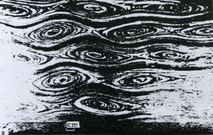
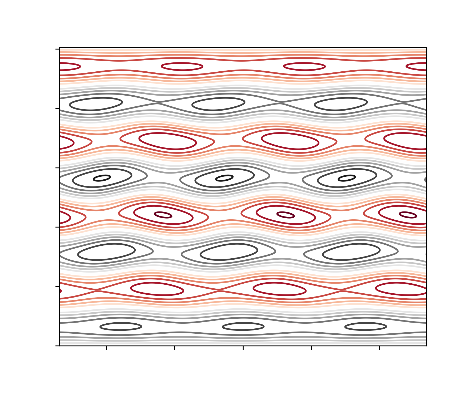
Figure 1: Top: Experimental secondary steady-state flow, with the Reynolds number slightly over the critical experimental Reynolds number 2000, given by Bandarenko [11, Figure 4] for $\lambda=20$ $k_{x}=0.68\pm 0.05$. Bottom: The secondary flow derived in Theorem 3.1 for $\lambda=20$, $k_{x}=0.7$, $N=4$, $j=1$, $-3\pi/k_{x}\leq x\leq 3\pi/k_{x}$, $0\leq y\leq 2N\pi$ and $R=1810$, which is over the analytic critical Reynolds number $R_{c}=1760$.

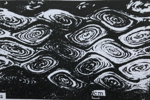
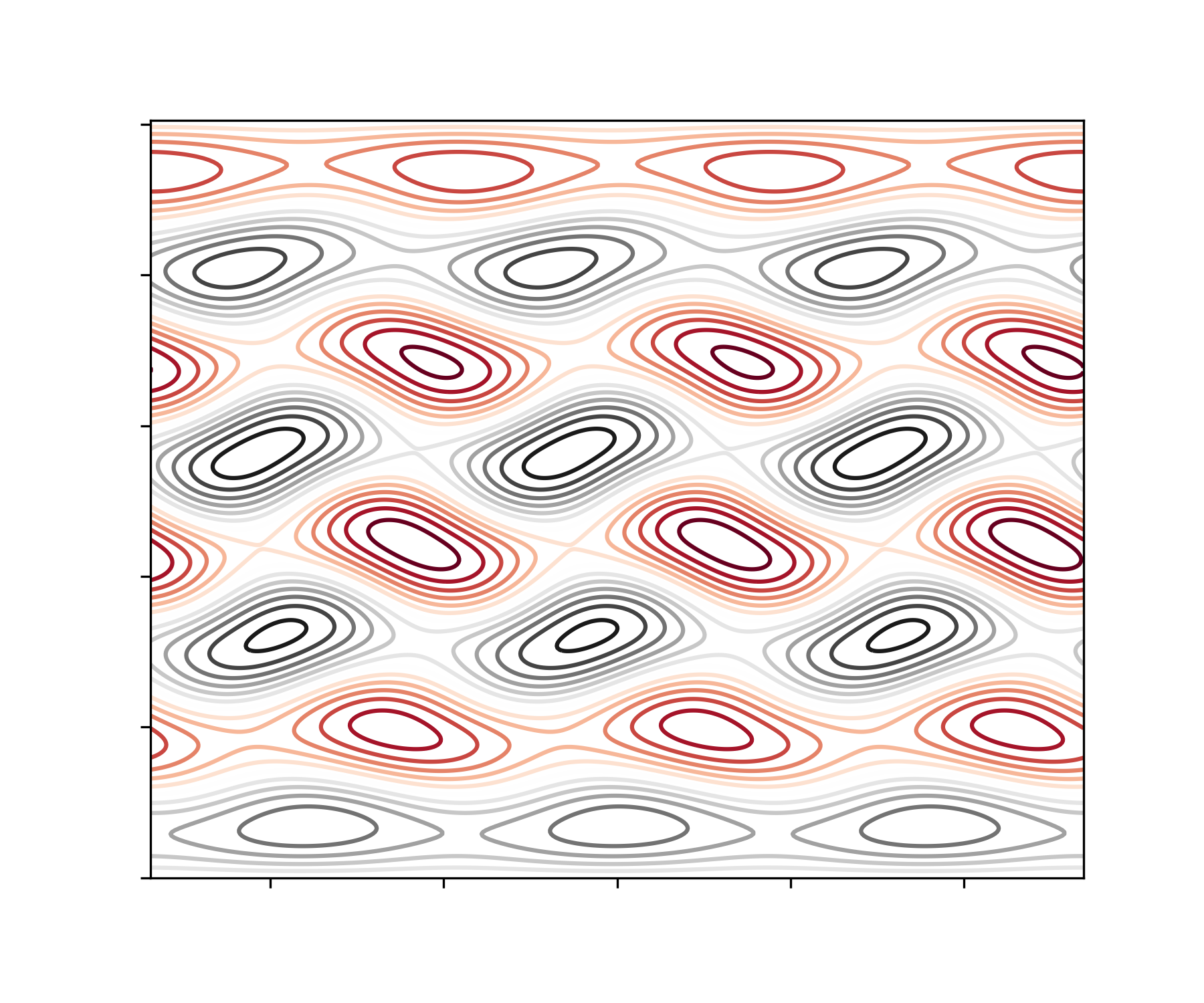
Figure 2: Top: Experimental flow pattern [11, Figure 5] at $R=1.25\times 2000$, well above the experimental critical value $2000$. Bottom: The secondary flow derived in Theorem 3.1 for $\lambda=20$, $k_{x}=0.7$, $N=4$, $j=1$, $-3\pi/k_{x}\leq x\leq 3\pi/k_{x}$, $0\leq y\leq 2N\pi$ and $R=2300$, which is well above the analytic critical Reynolds number $R_{c}=1760$.

It has been given in [21] that it is suitable to take $N=4$ and $j=1$ to get numerical flow comparable with experimental secondary flow in Figures 1 and 2. When $N=4$ and $j=1$, the first critical Reynolds number for the (8) and (9) in the wall-bounded domain is about 1768 (see [21]), which is reached at the wave number $k_{x}=0.63$. Now we take $k_{x}=0.7$ due to $k_{x}=0.68\pm 0.05$ in [11]. The secondary steady-state flow is dependent of the phase number $\theta\in[0,2\pi)$ and is generated by the eigenfunction $\psi_{\theta}$ and the basic flow $\sin y$. Therefore by the phase transition $x+\theta/k_{x}\to x$, the secondary flow at $\theta$ becomes the secondary flow at $0$. Therefore flow patterns of the solutions are same after the phase transformation $x+\theta/k_{x}\to x$. The experimental and numerical results at the present spectral method are displayed in Figures 1 and 2, which show respectively favorable agreement with the experiment measurements observed by Bonderanko et al. [11] for Reynolds number slightly over critical value (Figure 1) and well above critical value (Figure 2). The analytic solution in Figure 2 is also in a good agrement with experiment measurement of Burgess [12, Figure 1] or Figure 3 for the secondary Kolmogorov flow pattern in a soap film when $R$ is well above the critical Reynolds number of the laboratory experiment therein.

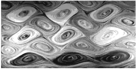
Figure 3: Experimental measurement for a soap film image well above the primary instability given by Burgess et al. [12, Figure 1].

Further numerical manipulations are performed with respect to the increment of high Reynolds number and different values of wave number $k_{x}$. Turbulence behaviours are observed for large values of $R$. In contraction to the laminar flow displayed in Figure 2 insensitive to initial data, the turbulence flow in high Reynolds number is very sensitive to the choice of initial data and time $t$. Flow patterns transited from the secondary steady states become more and more complex as $R$ increases. Figure 3 shows an example for four well developed flow patterns initially from four different initial data when $R=40000$, $k_{x}=0.7$, $\lambda=20$, $N=4$ and $j=1$.

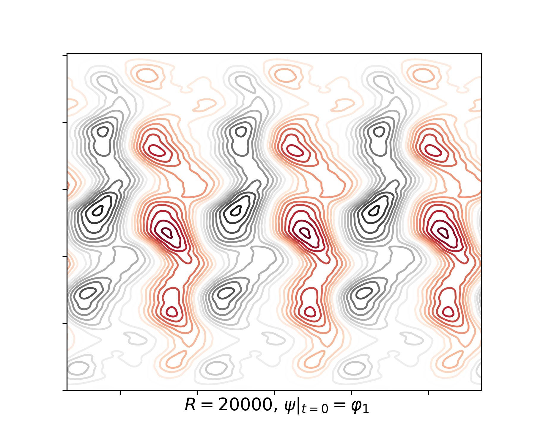
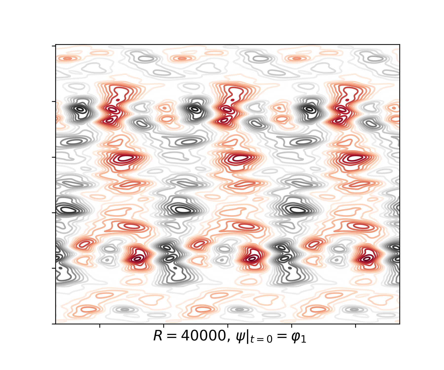
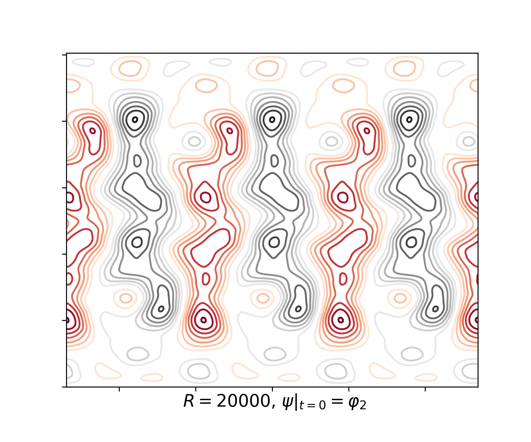
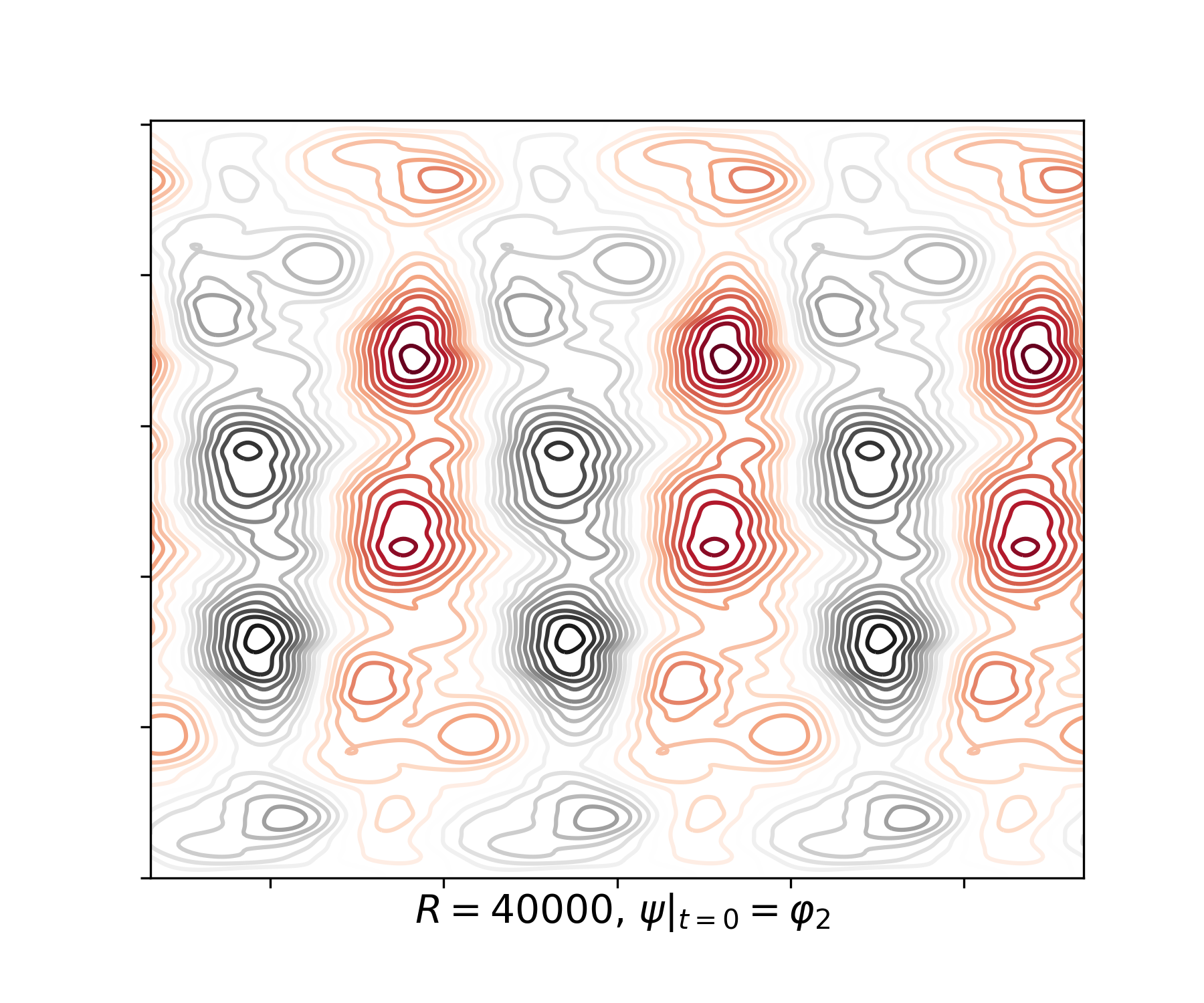
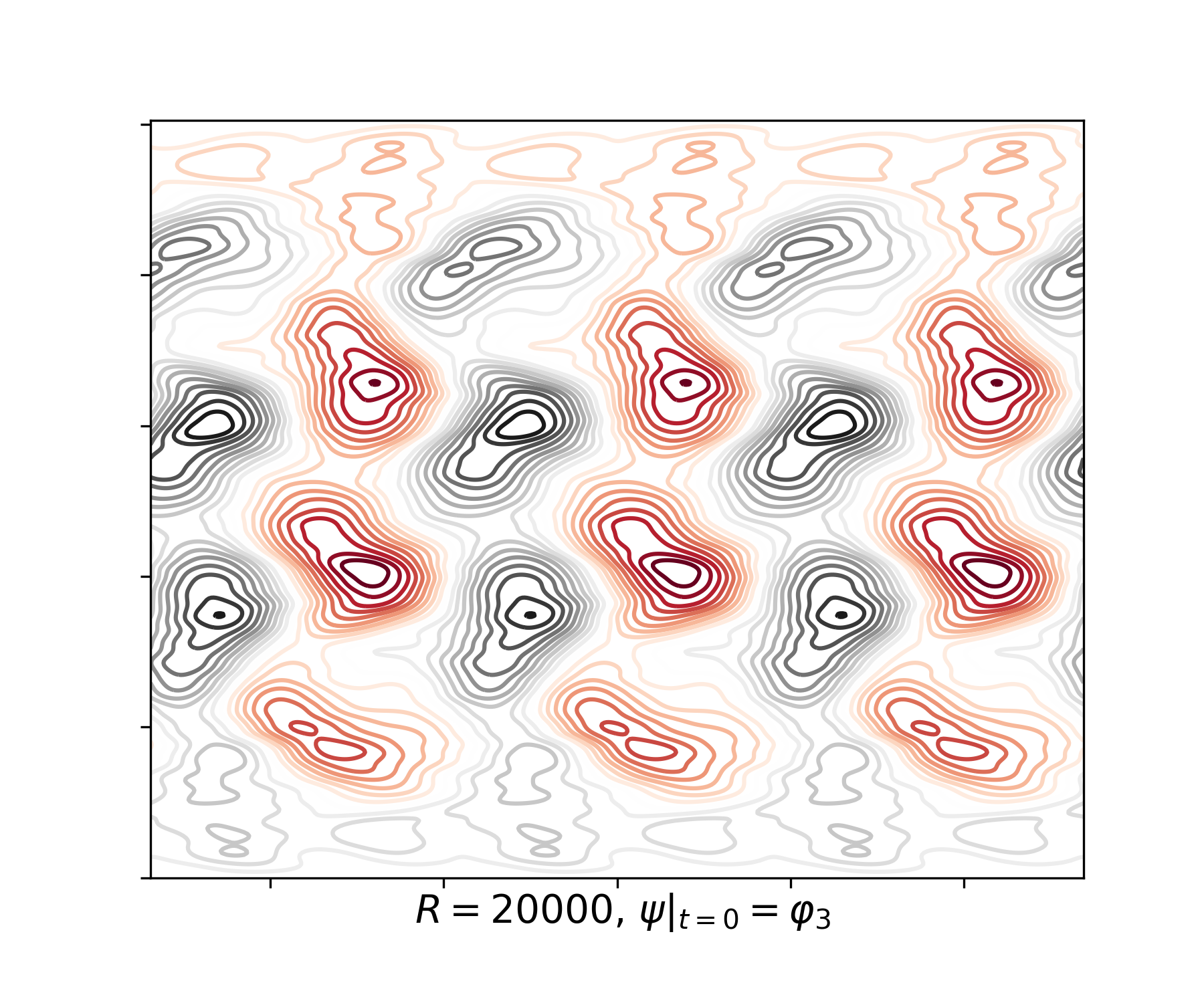
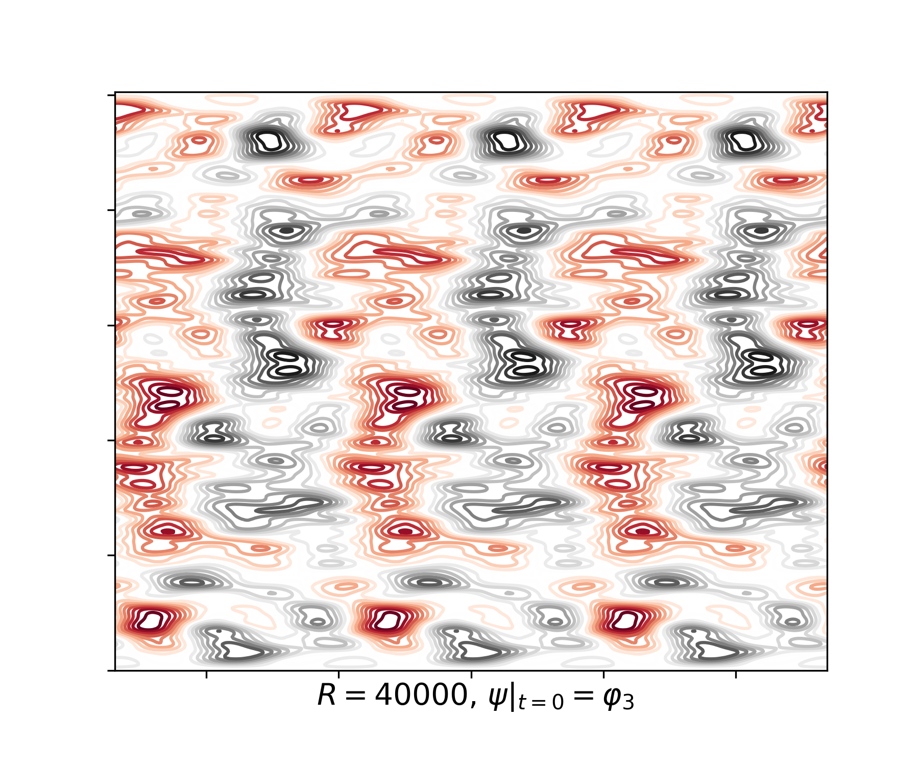
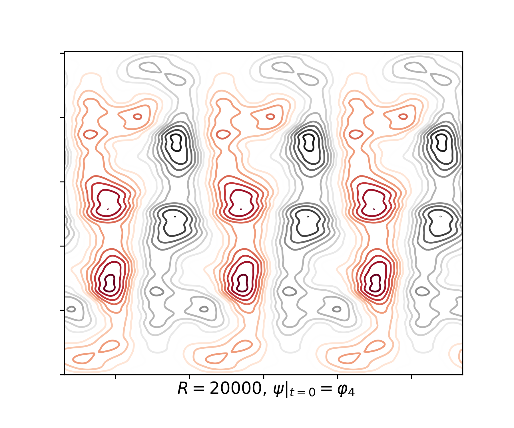
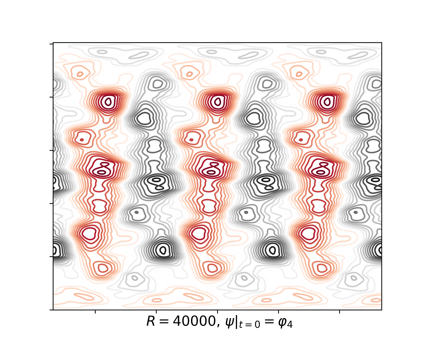
Figure 4: Numerical flow patterns of a solution $\psi$ to (8)-(9) developed from some different initial data $\varphi_{1},...,\varphi_{4}$ at the same time $t>>0$ and $R=20000,40000$ ( $\lambda=20$, $N=4$, $j=1$, $-3\pi/k_{x}<x<3\pi/k_{x}$, $0<y<2N\pi$).

5 Conclusions

In MHD laboratory experiments performed by Kolesnikov [13, 14] and Bondarenko et al. [11], an electrically conducting fluid flow is driven by the Lorenz force and controlled by Hartmann layer friction. This flow is governed by a two-dimensional equation (see Bondarenko et al. [11]) and is bounded by the lateral walls of an extended duct (see Thess [18]). The Kolmogorov flow is the basic steady-state solution of the MHD equation.

We prove rigorously that the MHD equation admits multiple secondary steady-state flows in relation to Bondarenko et al. [11] and confirm the finding of Chen and Price [21] on the secondary flows defined by a simple spectral truncation scheme. The difficulty in the analysis is due to the absence of flow invariant subspace of the ducted flow containing a single linear eigenfunction.

The bifurcating solutions in the Fourier expansion satisfies (60), which indicates the secondary flows being dominated by a small number of Fourier modes. This also implies that the energy dissipation of the MHD flow is mainly controlled by the Hartmann layer friction effect.

The theoretical secondary flow is in a good agreement with the experimental secondary flow observed by Bondarenko et al. [11] for $R=O(10^{3})$. Numerical simulation is performed for further transition of the secondary flow. When $R=O(10^{4})$, it is transited to well developed turbulence.

Acknowledgement. This work was partially supported by NSFC of China (11571240).

References

• [1] Reynolds O. 1883 An experimental investigation of the circumstances which determine whether the motion of water shall be direct or sinuous, and of the law of resistance in parallel channels. Phil. Trans. R. Soc. Lond. 174, 935-982.
• [2] Bedrossian J, Germain P and Masmoudi N. 2017 On the stability threshold for the 3D Couette flow in Sobolev regularity. Annals Math. 185, 541-608.
• [3] Li L, Wei D and Zhang Z. Pseudospectral bound and transition threshold for the 3d kolmogorov flow. arXiv:1801.05645.
• [4] Wei D and Zhang Z. Transition threshold for the 3d couette flow in Sobolev space. arXiv:1803.01359.
• [5] Arnold V I and Meshalkin L D. 1960 Seminar led by A. N. Kolmogorov on selected problems of analysis (1958-1959). Russ. Math. Surv. 15, 20-24.
• [6] Meshalkin L D and Sinai I G. 1961 Investigation of the stability of a stationary solution of a system of equations for the plane movement of an incompressible viscous liquid. J. Appl. Math. Mech. 25, 1700-1705.
• [7] Iudovich V I. 1965 Example of the generation of a secondary stationary or periodic flow when there is loss of stability of the laminar flow of a viscous incompressible fluid. J. Appl. Math. Mech. 29, 527-544.
• [8] Belotserkovskii S O, Mirabel A P and Chusov M A. 1978 On the Construction of the post-critical mode for a plane periodic flow. Izvestiya Atmos. Oceanic Phys. 14, 6-12.
• [9] Batchaev A M. 1988 Experimental Investigation of supercrticial Kolmogorv flow regimes on a cylindrical surface. Izvestiya Atmos. Oceanic Phys. 24, 614-619.
• [10] Batchaev AM and Dowzhenko VA. 1983 Experimental modeling of stability loss in periodic zonal flows. Dokl. Akad. Nauk. 273, 582-584.
• [11] Bondarenko N F, Gak M Z and Dolzhanskiy F V. 1979 Laboratory and theoretical models of a plane periodic flow. Izvestiya Atmos. Oceanic Phys. 15, 711-716.
• [12] Burgess J M, Bizon C, McCormick W D, Swift J B and Swinney H L. 1999 Instability of the Kolmogorov flow in a soap film. Physical Review E 60, 715-721.
• [13] Kolesnikov Y B. 1985 Experimental investigation of instability of plane-parallel shear flow in a magnetic field. Magnitnaya Gidrodinamika 60, 60-66.
• [14] Kolesnikov Y B. 1985 Instabilities and Turbulence in Liquid Metal Magnetohydrodynamics. Ph.D. thesis, University of Riga.
• [15] Obukhov A M. 1983 Kolmogorov flow and laboratory simulation of it. Russ. Math. Surv. 38, 113-126.
• [16] Tithof J, Suri B, Pallantla R K, Grigoriev R O and Schatz M F. 2017 Bifurcations in a quasi-two-dimensional Kolmogorov-like flow. J. Fluid Mech. 828, 837-866.
• [17] Sommeria J and Moreau R. 1982 Why how and when MHD turbulence becomes two-dimensional. J. Fluid Mech. 27, 507-518.
• [18] Thess A. 1992 Instabilities in two-dimensional spatially periodic flows. Part I. Kolmogorov flow. Phys. Fluids A 4, 1385-1395.
• [19] Thess A. 1990 Contributions to the Theory of Electromagnetically Driven Flows. Ph.D. thesis, Dresden: Technische UniversitΓ€t.
• [20] Chen Z M and Price W G. 2002 Supercritical regimes of liquid-metal fluid motions in electromagnetic fields: wall-bounded flows. Proc. R. Soc. A 458, 2735-2757.
• [21] Chen Z M and Price W G. 2005 Secondary fluid flows driven electromagnetically in a two-dimensional extended duct. Proc. R. Soc. A 461, 1659-1683.
• [22] Chen Z M. 2012 A vortex based panel method for potential flow simulation around a hydrofoil. J. Fluids Struct. 28, 378-391.
• [23] Frenkel A L. 1991 Stability of an oscillating Kolmogorov flow. Phys. Fluids A 3, 1718-1729.
• [24] Zhang X. 1995 On Linear and Nonlinear Stability Theory of Periodic Flows of Incompressible Fluid. Ph.D. thesis, Tuscaloosa: University of Alabama.
• [25] Zhang X and Frenkel A L. 1998 Large-scale instability of generalized oscillating Kolmogorov flows. SIAM J. Appl. Math. 58, 540-564.
• [26] Krasnoselskii M A. 1965 Topological methods in the theory of nonlinear integral equations. New York: Macmillan.
• [27] Rabinowitz P H. 1968 Existence and nonuniqueness of rectangular solutions of the BΓ©nard problbm. Arch. Rational Mech. Anal. 29, 32-57.
• [28] Rabinowitz P H. 1971 Some global results for nonlinear eigenvalue problem. J. Func. Anal. 7, 487-513.
• [29] Ma T and Wang S. 2003 Attractor bifurcation theory and its applications to Rayleigh BΓ©nard convection, Commun. Pure Appl. Anal. 2, 591-599.
• [30] Ma T and Wang S. 2014 Phase Transition Dynamics. New York: Springer.
• [31] Wall H S. 1948 Analytic Theory of Continued Fractions. New York: D. Van Nostrand.
• [32] Khinchin A Y. 1964 Continued Fractions. Chicago: University of Chicago Press.