$\Lambda p$ Elastic Scattering in the CLAS Detector

Abstract

The elastic scattering process $\Lambda p\to\Lambda p$ offers insights on multiple problems in nuclear physics. $\mathrm{SU}(3)_{F}$ symmetry implies a close agreement between the $\Lambda p$ and $pp$ scattering cross sections. The $\Lambda p$ elastic scattering cross section can also illuminate the structure of neutron stars. A data-mining project was started using multiple CLAS data sets taken for other purposes with photon beams on a long liquid hydrogen target. A $\Lambda$ produced in a process such as $\gamma p\to K^{+}\Lambda$ can interact with a second proton inside the target before either decaying or leaving the target. The good angular acceptance and momentum resolution of CLAS make it well-suited for this type of analysis, even though it was not designed for such a measurement. The scattered $\Lambda$ can be identified from the $\pi^{-}p$ invariant mass. The four-vector of the initial $\Lambda$ is then reconstructed in the process $Xp\to\Lambda p$, which shows a strong peak at the $\Lambda$ mass with roughly twice the number of events as the existing world data sample. This observation opens up the possibility of other measurements using secondary beams of short-lived particles. This paper will discuss the current status of the analysis, and our plans for future work on this project.

1 MOTIVATION

The hyperon-nucleon interaction is of fundamental importance in both nuclear physics and astrophysics. The so-called “hyperon puzzle” in neutron star structure is based, in part, on experimental measurements of the hyperon-nucleon cross section, which are badly in need of improvement. $\mathrm{SU}(3)_{F}$ symmetry, a powerful tool in nuclear physics, treats all hadrons in the same SU(3) multiplet as different manifestations of the same particle. This implies a relationship between the $\Lambda N$ and $NN$ interactions that has only been poorly tested. One of the main reasons for this is the short lifetime of the hyperons. The longest-lived hyperon, the $\Lambda$, has a decay length given by $c\tau_{\Lambda}=7.89\,\mathrm{cm}$.

To improve the state of our understanding of this interaction, we have developed a new technique, in which the incident $\Lambda$ (referred to here as the “beam” $\Lambda$) is produced via a process such as $\gamma p\to K^{+}\Lambda$. The beam $\Lambda$ can then interact with a second proton inside the target before either decaying or leaving the target. This technique has never been attempted before with a photon beam.

1.1 The Hyperon Puzzle

A neutron star is a gravitationally bound massive object, primarily consisting of neutrons. As the mass of such an object increases, the Pauli pressure of the nucleons (effectively, the chemical potential of the neutrons in the star) also increases. At high enough masses, this pressure can be relieved by the transmutation of neutrons into hyperons. This has the effect of softening the neutron star’s equation of state (EoS), reducing the maximum mass a neutron star can attain before collapsing to a black hole. Many EoS calculations lead to a maximum mass that is less than the masses of already-observed neutron stars.

The conflict between the theoretical expectation of the existence of hyperons in neutron stars and the effect that existence has on the EoS and, in turn, the maximum observed mass, is known as the hyperon puzzle. There have been many theoretical attempts to resolve the hyperon puzzle. These focus primarily on introducing a repulsive force, often due to the $\Lambda NN$ interaction, to help to stiffen the EoS.[1] However, more data are needed to constrain the hyperon-nucleon interaction.

1.2 $\mathrm{SU}(3)_{F}$ Symmetry

The strong nuclear interaction is governed by the QCD Lagrangian ${\cal L}_{QCD}$, which can be rewritten as the sum of two terms [2]:

$${\cal L}_{QCD}={\cal L}_{0}+{\cal L}_{m},$$ (1)

where ${\cal L}_{m}$ represents the single term that depends on the quark mass $\sum_{q}\overline{\psi}_{q,a}m_{q}\delta_{ab}\psi_{q,b}$, and ${\cal L}_{0}$ contains the rest of the Lagrangian. In the limit of massless quarks, the QCD Lagrangian reduces to the ${\cal L}_{0}$ term. This leads to the prediction that, in this limit, all of the baryons in a given multiplet will have the same mass, and have similar properties. Baryons in different multiplets will have different masses from each other, due to the dynamics of the strong interaction. Within each multiplet, we find that the different masses of the baryons are determined by the mass term ${\cal L}_{m}$.

This relatively simple idea works surprisingly well. We find, for instance, that the mass splitting between the ground-state and the first excited-state nucleon, the N(1440), is approximately 500 MeV. The corresponding mass splitting in the $\Lambda$ sector compares the ground-state $\Lambda(1115)$ to the first excited-state (octet) $\Lambda$, the $\Lambda(1600)$, for a splitting of 485 MeV. The difference in these mass splittings is only 15 MeV, remarkably close for strong interaction calculations.

A similar comparison can be made for cross sections of processes related by $\mathrm{SU}(3)_{F}$ symmetry. Figure 1 shows the cross section for the processes $\pi^{-}p\to n\eta$ and $K^{-}p\to\Lambda\eta$.

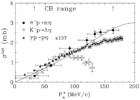
Figure 1: The $p^{*}_{\eta}$ dependence of $\sigma^{tot}(\pi^{-}p\to\eta n)$, $\sigma^{tot}(K^{-}p\to\eta\Lambda$), and $\sigma^{tot}(\gamma p\to\eta p$). Experimental data for $\pi^{-}p\to n\eta$ (filled circles) are from [3]; data for $K^{-}p\to\eta\Lambda$ (open circles) are from [4], and data for $\gamma p\to\eta p$ (stars) are from [5]. The photoproduction data have been multiplied by a factor of 137. The solid line shows the FA02 prediction of Ref. [6].

As seen in the Figure, the cross sections for the two processes $\pi^{-}p\to n\eta$ and $K^{-}p\to\Lambda\eta$ are nearly identical near the threshold, when plotted as a function of the center-of-mass momentum of the $\eta$.

This leads to the prediction that the cross sections for other processes related by $\mathrm{SU}(3)_{F}$ symmetry should be similarly related. This can be studied, for instance, in the processes $pp\to pp$ and $\Lambda p\to\Lambda p$. A hint of the relationship between these processes is evident in the Additive Quark Model of Levin and Frankfurt [7]. Using this model, one obtains the following relationship:

$$\sigma_{\Lambda p}=\frac{1}{2}\left(\sigma_{pp}+\sigma_{\Xi p}\right)$$ (2)

While this model is best-suited to high-energy measurements, it is still a good place to start.

1.3 Previous Measurements

The present state of the data for the process $\Lambda p\to\Lambda p$ is poor. Figure 2 shows the state of cross section measurements for the processes $pp\to pp$; Fig. 3 shows the equivalent cross section data for $\Lambda p\to\Lambda p$.

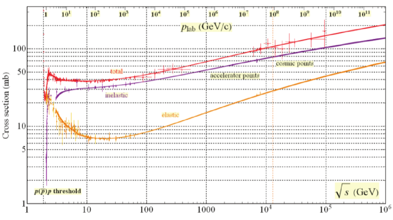
Figure 2: The existing data for the process $pp\to pp$, from Ref. [2].

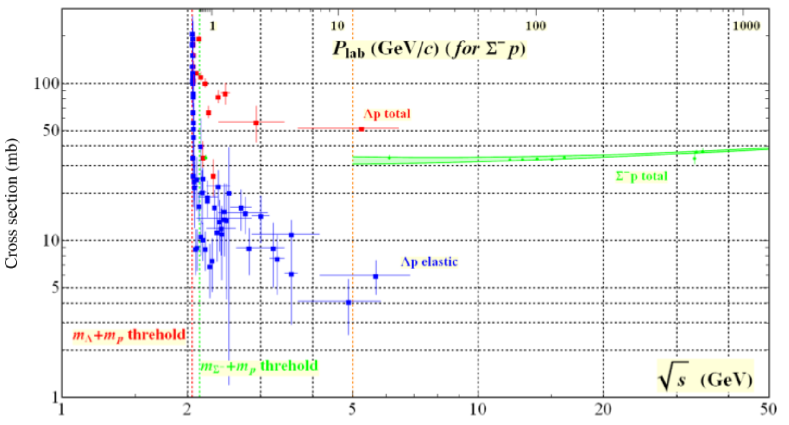
Figure 3: The existing data for the process $\Lambda p\to\Lambda p$ (bottom), from Ref. [2].

As seen in the figures, the quality of the data for the process $pp\to pp$ is of much higher quality than that for $\Lambda p\to\Lambda p$.

The present world data sample for the process $\Lambda p\to\Lambda p$ consists of thirteen publications.[8, 9, 10, 11, 12, 13, 14, 15, 16, 17, 18, 19, 20] Table 1 summarizes the existing world data set for this process.

Table 1: The existing data for the process $\Lambda p\to\Lambda p$.

Reference	$\Lambda$ source	Detector	$p_{\Lambda}$	$N_{\Lambda p\to\Lambda p}$
Crawford et al. [8]	$\pi^{-}p\to\Lambda K^{0}$	LH2 BC	0.5–1.0	4
Alexander et al. (1961) [9]	$\pi^{-}p\to\Lambda K^{0}$	LH2 BC	0.4–1.0	14
Groves [10]	$K^{-}N\to\Lambda\pi$	Propane BC	0.3–1.5	26
Beillière et al. [11]	$K^{-}N\to\Lambda\pi$	Freon BC	0.5–1.2	86
Piekenbrock and Oppenheimer [12]	$K^{-}A\to\Lambda X$	Heavy Liquid BC	0.15–0.4	11
Sechi-Zorn et al. (1964) [13]	$K^{-}p\to\Lambda X$	LH2 BC	0.12–0.4	75
Vishnevksiĭ et al. [14]	$nA\to\Lambda X$	Propane BC	0.9–4.7	12
Bassano et al. [15]	$K^{-}p\to\Lambda X$	LH2 BC	1.0–5.0	68
Alexander et al. (1968) [16]	$K^{-}p\to\Lambda X$	LH2 BC	0.1–0.3	378
Sechi-Zorn et al. (1968) [17]	$K^{-}p\to\Lambda X$	LH2 BC	0.1–0.3	224
Kadyk et al. [18]	$K^{-}\mathrm{Pt}\to\Lambda X$	LH2 BC	0.3–1.5	175
Anderson et al. [19]	$p\mathrm{Pt}\to\Lambda X$	LH2 BC	1.0–17.0	109
Mount et al. [20]	$p\mathrm{Cu}\to\Lambda X$	LH2 BC	0.5–24.0	71

There have been a total of less than 1300 observed $\Lambda p\to\Lambda p$ events. All of the experiments used bubble chambers, which limited the rate at which data could be taken. In all of the previous measurements, the incident $\Lambda$ is created inside a bubble chamber via some other process (the “$\Lambda$ source” column in Table 1; the $\Lambda$ then interacts with a proton within the bubble chamber to produce the $\Lambda p\to\Lambda p$ event.

2 DATA-MINING PLAN

A similar approach to this process could be successful today. While the detectors in common usage today do not allow the complete visualization of events afforded by the bubble chambers used in the older experiments, they have the advantage of significantly higher rates.

In comparison with the previous data, $\Lambda$s are produced in far more plentiful quantities in modern experiments using liquid hydrogen targets. Because the $\Lambda$ lives for a short time before decaying, it can interact with a second proton inside the same target. With a $4\pi$ detector, all the final-state particles can be observed, allowing the reconstruction of the entire event.

The CLAS detector [21], at the Thomas Jefferson National Accelerator Facility (JLab) in Newport News, VA, was originally built to study the structure of the proton and its excited states. It is well-suited for this task. It has good angular and momentum resolution, as well as good angular and momentum acceptance. It also has a good efficiency for multiparticle final states. Even though it was never conceived for such a process, it is difficult to imagine a detector that could do a much better job.

In its original layout, the JLab accelerator produced an electron beam of energies up to 6 GeV in CLAS. This electron beam was used to produce a photon beam with a bremsstrahlung tagging system. The process that produced the beam $\Lambda$ was not identified; the simplest such process is $\gamma p\to K^{+}\Lambda$. The complete event topology assuming this production mechanism is shown in Fig. 4.

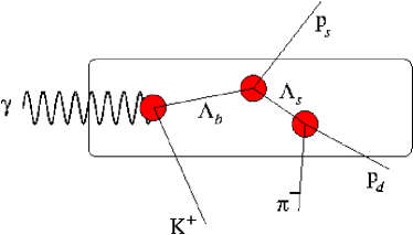
Figure 4: The event topology for the process $\gamma p\to K^{+}\Lambda;\,\Lambda p\to\Lambda p$ considered in this work.

With this in mind, a survey of the available data taken by the CLAS Collaboration was made, to determine a likely dataset in which this event could be observed. To decide which dataset to begin this study with, we looked for one with a large integrated luminosity, with a long liquid hydrogen target to facilitate the rescattering process.

The CLAS g12 run, taken in the Spring of 2008, was chosen for this work. It used a photon beam with energies up to $5.4\,\mathrm{GeV}$, and took a total of approximately $52\,pb^{-1}$ of $\gamma p$ data. It had a 40-cm-long liquid hydrogen target, which gives a large number of potential secondary scattering targets. The cross section for the basic production process $\gamma p\to K^{+}\Lambda$ is approximately $0.5\,\mu b$; there were thus approximately $2.6\times 10^{7}$ beam $\Lambda$s for this analysis.

For the process of interest,

$$\gamma p\to K^{+}\Lambda;\ \Lambda p\to\Lambda p$$

the final state was $K^{+}\pi^{-}pp$. The presence of two protons in the final state, an “apparent” violation of baryon conservation, resulted in an extremely restrictive cut, which essentially required that some form of rescattering has taken place.

By skimming the data for events with two protons, the size of the dataset was reduced from 126 TB to approximately 4 TB. This reduced dataset could then be analyzed in its entirety very quickly.

3 EVENT SELECTION

The data analysis consisted of reconstructing the event from the final state. We began by looking for the scattered $\Lambda$ (“$\Lambda_{s}$”) in the $\pi^{-}p$ invariant mass. Because there were two protons in the final state, there were two such invariant masses to be checked. For simplicity, we took the invariant mass closest to $m_{\Lambda}=1.115\,\mathrm{GeV}$ to indicate which was the “correct” proton. This spectrum is shown in the left plot of Fig. 5.

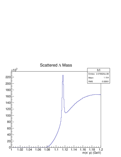
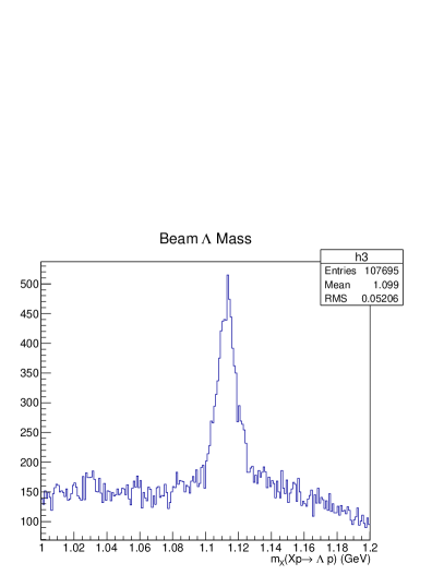
Figure 5: Analysis spectra for $\Lambda p$ elastic scattering. One-half of the CLAS g12 dataset (approximately 25 $\mathrm{pb}^{-1}$ was used in this analysis. No attempt has yet been made to reduce the background. (left) The invariant mass $m_{X}$ of the $\pi^{-}p$ system. Only the invariant mass closest to $m_{\Lambda}=1.115\,\mathrm{GeV}$ is plotted. (right) The missing mass $m_{X}$ for the process $Xp\to\Lambda p$.

The scattered $\Lambda$ shows up as an unmistakable peak above a large background which we have not yet attempted to reduce.

If the $\Lambda$ found in this procedure was actually the scattered $\Lambda$ in the process $\Lambda p\to\Lambda p$, the second proton provided all the remaining information needed to completely reconstruct the event. The beam $\Lambda$ was then the missing particle in the process $Xp\to\Lambda p$, and should show up in the corresponding missing mass plot. This is shown in the right plot of Fig. 5. While we have not done a detailed analysis of this plot, it is clear that there are more than twice the number of events in the peak as are in the entire world data sample.

4 CROSS SECTION CALCULATION

The determination of the cross section for this process is more complicated than for a typical process in nuclear physics. The equation for the cross section is given by

$$\sigma=\frac{N_{e}}{N_{b}N_{t}A\eta}=\frac{N_{e}}{{\cal L}A\eta},$$

where $N_{e}$ is the number of detected events; $N_{b}$ and $N_{t}$ are the number of beam and target particles, respectively; $A$ is the detector acceptance; and $\eta$ is a catch-all factor for any analysis inefficiencies.

The product $N_{b}N_{t}$ is often referred to as the luminosity ${\cal L}$, and is a measure of the total amount of data available. For a typical experiment, $N_{b}$ is determined by various beam diagnostic equipment, either by the accelerator or, in the case of tagged secondary beams, by the beam tagger system diagnostics. The number of target particles $N_{t}$ is typically calculated using the measured length of the target, multiplied by appropriate factors of the target density, atomic mass number, and Avogadro’s number $N_{A}=6.02\times 10^{23}$.

We cannot use such simple diagnostic for $N_{b}$, however. There is no “beam diagnostic” that can count the number of $\Lambda$s produced in our detector. Since the $\Lambda$ is neutral, and decays quickly, it cannot be measured directly. While it is possible to “tag” the $\Lambda$ in specific processes, such as $\gamma p\to K^{+}\Lambda$, there are many other processes that can produce $\Lambda$s in our target.

We also cannot use the target length to determine $N_{t}$, for three reasons. First, the beam $\Lambda$ is created within the target; any protons upstream of the $\Lambda$ production vertex are not available for later scattering. Second, the $\Lambda$ will decay after a short time; any protons downstream of the $\Lambda$ decay vertex are also unavailable for later scattering. Third, unlike the beam produced by the accelerator, the beam $\Lambda$ is not traveling parallel to the target axis. It can leave the target through the cylindrical wall long before traversing the entire target length.

The best that can be done with respect to $N_{b}$ is an estimate of the number of beam $\Lambda$s. For our first attempt at this, we will focus on the $\Lambda$ photoproduction process $\gamma p\to K^{+}\Lambda$. Figure 6 shows the kinematics of the $\Lambda$ in the process $\gamma p\to K^{+}\Lambda$.

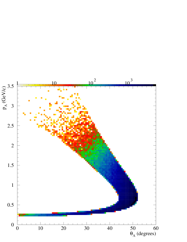
Figure 6: The kinematics of the outgoing $\Lambda$ in the process $\gamma p\to K^{+}\Lambda$, from simulation. The photon beam energy in the simulation was chosen to match the properties of the beam used in the CLAS g12 run.

This plot is based on the thrown values for the simulation. For this purpose, it is not necessary to actually perform the simulation; the entire calculation is based on the geometry of the target and the knowledge of the decay length of the $\Lambda$.

To accomplish this, it is necessary to rebin the data. We are interested in the flux of $\Lambda$s as a function of the $\Lambda$ momentum $p_{\Lambda}$ and the $\Lambda$ lab angle $\theta_{\Lambda}$. In the process $\gamma p\to K^{+}\Lambda$, however, the results are normally reported in terms of the photon energy $E_{\gamma}$ and the kaon c.m. angle $\theta^{*}_{K^{+}}$. The kinematics are overdetermined, so there is a straightforward relationship that will allow the rebinning of the data. Once this is complete, we can make an estimate of how many beam $\Lambda$s are in each of our kinematic bins, based upon previous measurements of the cross section for $\gamma p\to K^{+}\Lambda$.

The next step is to determine the effective target thickness. This must be done for each of the kinematic bins for our beam $\Lambda$; two $\Lambda$s with the same momentum will have different mean path lengths if they are traveling at different angles, since one will escape the target before the other, for instance. There are three possible reasons why the beam $\Lambda$ will not interact with a second proton in the target:

1. The beam $\Lambda$ decays before interacting. The mean path length of a $\Lambda$ of velocity $\beta$ before decaying is given by $\ell_{decay}=\beta\gamma c\tau$. This calculation ignores the possibility that the beam $\Lambda$ will leave the target before interacting with a proton, effectively assuming a target of infinite size.

2. The beam $\Lambda$ is produced at a large angle, and escapes the target through the cylindrical wall. For a particle produced with an angle $\theta_{\Lambda}$ relative to the target axis, the mean length from the production vertex to the cylindrical wall is given by $\ell_{cyl}=r_{tgt}/\sin{\theta_{\Lambda}}$. This calculation ignores the possibility that the beam $\Lambda$ will either decay or exit through the endcap, effectively assuming a target of infinite length.

3. The beam $\Lambda$ is produced at a small angle close to the downstream end of the target, and escapes through the endcap before decaying. For a particle produced a distance $z_{\Lambda}$ downstream of the entrance of a target of length $z_{tgt}$ with an angle $\theta_{\Lambda}$ relative to the target axis, the mean length from the production vertex to the $z$-position of the downstream endcap position of the target is given by $\ell_{end}=(\ell_{tgt}-z_{\Lambda})/\cos{\theta_{\Lambda}}$. This calculation ignores the possibility that the beam $\Lambda$ will either decay or exit through the cylindrical wall, effectively assuming a target of infinite radius.

The actual mean path for any given $\Lambda$ $\ell_{mean}$, taking into account the possibility that it will either decay or exit the target before interacting with a proton is the minimum of these three numbers: $\ell_{mean}=min(\ell_{decay},\ell_{cyl},\ell_{end})$. For the kinematics of the beam $\Lambda$ in the g12 dataset, Fig. 7 shows the distribution of all four variables $\ell_{decay}$ (top left), $\ell_{cyl}$ (top right), $\ell_{end}$ (bottom left), and $\ell_{mean}$ (bottom right).

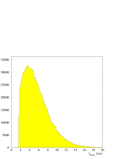
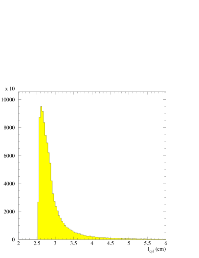
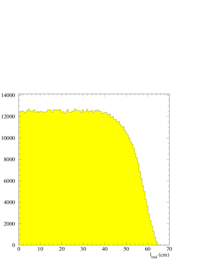
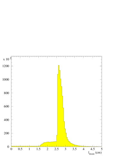
Figure 7: The mean path length of the beam $\Lambda$ in the g12 liquid hydrogen target. All values are taken from the kinematics of the $\gamma p\to K^{+}\Lambda$ process at the photon energies used in the g12 run. (top left) The mean distance traveled by a $\Lambda$ before decaying. (top right) The mean length traveled by a $\Lambda$ before escaping via the cylindrical wall of the target. (bottom left) The mean length traveled by a $\Lambda$ before escaping via the target endcap. (bottom right) The mean path length of all $\Lambda$s in this measurement, calculated as the minimum of the other three values.

What we see is that the majority of our $\Lambda$s are escaping through the cylindrical wall of the target. Using a long target does not, therefore, increase the mean path length of the $\Lambda$ noticeably (although it will increase the number of $\Lambda$s produced).

Having found both the number of beam $\Lambda$s $N_{b}$ and the effective target thickness $N_{t}$ as a function of the $\Lambda$ momentum $p_{\Lambda}$ and lab angle $\theta_{\Lambda}$, we then can calculate the luminosity for this measurement using the following equation:

$${\cal L}=\sum_{all\ bins}N_{b}(p_{\Lambda},\theta_{\Lambda})N_{t}(p_{\Lambda},\theta_{\Lambda})$$

The next step in the calculation of the cross section for $\Lambda p\to\Lambda p$ is to simulate the acceptance for this process, using the measured kinematics as input. This procedure is underway, with the expectation that it should be complete within the year.

5 FUTURE DIRECTIONS

Our success in this endeavor has motivated us to consider other ways in which this technique can be exploited with detectors such as CLAS. While we are still in the process of developing a new proposal to take advantage of the new capabilities of the CLAS12 detector with the higher energy beam now available at JLab, we are also looking into the existing data currently stored. This represents nearly twenty years of data acquisition, much of which is compatible with studies such as this.

Our experience with this measurement makes it clear that a long target is not necessary for such an experiment. Because the beam particles nearly always escape the target through the cylindrical walls, the target length only contributes to the measurement through the number of beam particles produced. We are therefore free to look at all previous datasets for this work.

In principle, any particle produced in sufficient quantities may be used for such a study. To begin with, we will focus on processes that include two protons in the final state. This will allow us to make use of the skimmed data already in hand for the $\Lambda p\to\Lambda p$ study. Such a skim reduces the size of the background considerably; from an original size of 230TB, the final skimmed dataset is slightly more than 4TB.

5.1 Measurement of $\gamma p\to\Lambda X$

At the present time, we must restrict ourselves to events in which we can identify the $K^{+}$ from the process $\gamma p\to K^{+}\Lambda$. The reason for this is that this process is well-studied, and its cross section is well-known. However, it is a relatively small part of the total $\Lambda$ production cross section at higher energies. In order to take advantage of all of the $\Lambda$s produced in CLAS, it will be necessary to measure the process $\gamma p\to\Lambda X$. This is one of our first plans after the present analysis is complete, which will increase greatly the number of beam $\Lambda$s at our disposal.

5.2 Confirmation of the $\Lambda p$ scattering result

Our first effort was to duplicate the measurements made with the g12 dataset. For this, we look at the g11 dataset. This set was taken in 2004, and used the same 40-cm-long $\mathrm{LH}_{2}$ target as the g12 dataset. The photon energy range was slightly lower, and the trigger was different, which will affect the events seen by CLAS.

The plots in Fig. 8 are the same as those in Fig. 5, except taken with the g11 dataset.

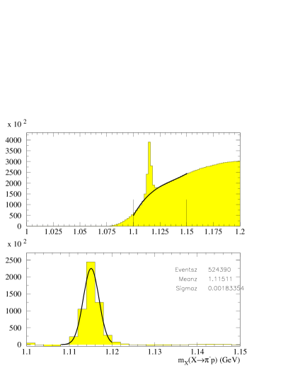
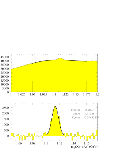
Figure 8: Analysis spectra for the analysis of $\Lambda p$ elastic scattering, from the g11 dataset. No attempt has yet been made to reduce the background. The units for all plots are GeV. (left plots) The invariant mass $m_{\pi^{-}p}$ of the $\pi^{-}p$ system. Only the invariant mass closest to $m_{\Lambda}=1.115\,\mathrm{GeV}$ is plotted. The scattered $\Lambda$ shows up as a strong peak above the background. (right plots) The missing mass $m_{X}$ for the process $Xp\to\Lambda p$. Only events with $m_{\Lambda_{s}}$ within 5 MeV of the known value of $m_{\Lambda}=1.115\,\mathrm{GeV}$ are used. (top plots) The raw invariant/missing mass spectra. The dark line is a 3rd-order polynomial fit to the background. (bottom plots) The same plot, with the background subtracted. The dark line is a gaussian fit to the remaining peak.

Here, the plots on the left are the invariant mass plots of the $\pi^{-}p$ system, where only the invariant mass closest to $m_{\Lambda}=1.115\,\mathrm{GeV}$ is plotted. The scattered $\Lambda$ shows up very strongly as a peak above the background in the top left plot. For events with $m_{\Lambda_{s}}$ within 5 MeV of the known value of $m_{\Lambda}=1.115\,\mathrm{GeV}$, the missing mass $m_{X}$ for the process $Xp\to\Lambda p$ is shown in the right plots. While the background in the top right plot is admittedly very large, there is clearly a peak above the background. The dark line in the top plots is a fit to a 3rd-order polynomial background. In the bottom plots in the Figure, the background has been subtracted, and the remaining peak has been fit with a gaussian. Note that the bottom right plot shows 17,000 events, which is more than an order of magnitude greater than the existing world data sample. The analysis of this dataset is still underway.

5.3 $pp$ Elastic Scattering

For other tests of this technique, we chose to take advantage of the skim performed in the context of the $\Lambda p$ rescattering pilot study. This skim required two protons in the final state. With this data skim, the simplest process that can be studied is $pp\to pp$. This process, shown in Fig. 2, has been measured very well; we do not expect to improve upon the existing data set. However, this is still a useful test of our cross section determination for the $\Lambda p$ cross section.

The analysis of $pp$ elastic scattering is slightly different than that of $\Lambda p$ scattering, in that the scattered proton is detected directly, and need not be reconstructed. The only analysis to be done here is to identify the two final-state protons, and to look for a peak at the proton mass in the missing mass plot of the process $Xp\to pp$. This is shown in Fig. 9.

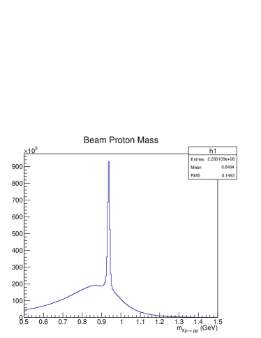
Figure 9: The missing mass $m_{X}$ in the process $Xp\to pp$ for the g12 dataset. The proton is strongly seen over a smooth background.

It should be pointed out here that the CLAS g12 trigger required three charged particles. Because of this, we do not have access to protons produced in the process $\gamma p\to\pi^{0}p$. Instead, the proton production process is $\gamma p\to\rho^{0}p$ or $\gamma p\to\omega p$, which clearly is still useful for studies of this sort.

5.4 $K_{s}p$ Elastic Scattering

Like the $\Lambda$, the $K_{s}$ is a very short-lived particle, with $c\tau=2.68\,\mathrm{cm}$.[2] There are even fewer cross section measurements for the process $K_{S}p\to K_{S}p$ than for $\Lambda p\to\Lambda p$; only one published measurement exists.[19] The complete process in the CLAS detector is $\gamma p\to K_{S}^{0}\Sigma^{+};K_{S}p\to K_{S}p$. The analysis of this process is complicated by the fact that, since we do not detect the beam $K_{s}$, there is contamination from the process $K_{L}p\to K_{S}p$, which will need to be subtracted from our result.

We have begun the analysis of this process by looking for the $K_{S}$ via its decay to $\pi^{+}\pi^{-}$. Figure 10 shows the invariant mass spectrum of $\pi^{+}\pi^{-}$, showing a strong peak above a smooth background.

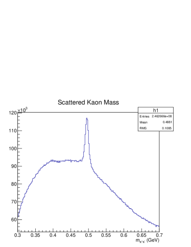
Figure 10: The invariant mass $m_{\pi^{+}\pi^{-}}$ of the $\pi^{+}\pi^{-}$ system in the g12 dataset. The $K_{S}$ is clearly seen over a smooth background.

This analysis is still in its infancy; we have yet to isolate the beam $K_{S}$ in the process $K_{S}p\to K_{S}p$, which is the next step.

5.5 $\Xi p$ Elastic Scattering

As mentioned previously, this technique could be used to test the Additive Quark Model of Levin and Frankfurt.[7] At the present time, we do not have a dataset large enough to see a useful number of events for this process. In the future, we hope to use the upgraded CLAS12 detector to address this question.

6 CONCLUSIONS

We have shown that it is possible to create a beam of short-lived particles to use in scattering processes on the proton. We have used this technique with the CLAS detector to produce a beam of $\Lambda$ hyperons, with which we have successfully identified the process $\Lambda p\to\Lambda p$ in two independent datasets. In so doing, we have increased the world data sample for this process by well over an order of magnitude.

Using the same dataset, we have shown that the process $pp\to pp$ is also accessible via CLAS data, and can be used to check the systematic uncertainty of the $\Lambda p\to\Lambda p$ cross section measurement. We have also shown that the luminosity, while not yet completely understood, is not an intractable problem.

Finally, this new technique opens up a whole new range of possible studies with the CLAS detector that were not considered previously. This will enable a large increase in the amount of physics output from CLAS in the future. There is a great deal of data available to test out new methods, which can then be more finely tuned by the proposal of dedicated experiments using this technique.

7 ACKNOWLEDGMENTS

This work was performed with the support of a grant from the US Department of Energy. This program is being pursued in collaboration with CSU Dominguez Hills undergraduate students Noraim Nuñez and Marcos Guillen, and with Dr. Ken Hicks and Joey Rowley from Ohio University.

References

- Lonardoni et al. [2015] D. Lonardoni et al., Phys. Rev. Lett. 114, p. 092301 (2015).
- Tanabashi et al. [2018] M. Tanabashi et al. (Particle Data Group), Phys. Rev. D 98, p. 030001 (2018).
- Prakhov et al. [2005] S. Prakhov et al. (Crystal Ball Collaboration), Phys. Rev. C 72, p. 015203 (2005).
- Starostin et al. [2001] A. Starostin et al. (Crystal Ball Collaboration), Phys. Rev. C 64, p. 055205 (2001).
- Krusche et al. [1995] B. Krusche et al., Phys. Rev. Lett. 74, p. 3736 (1995).
- Arndt et al. [2004] R. Arndt et al., Phys. Rev. C 69, p. 035213 (2004).
- Levin and Frankfurt [1965] E. Levin and L. Frankfurt, Pisma ZhETP 3, p. 105 (1965).
- Crawford et al. [1959] F. Crawford et al., Phys. Rev. Lett. 2, p. 174 (1959).
- Alexander et al. [1961] G. Alexander et al., Phys. Rev. Lett. 7, p. 348 (1961).
- Groves [1963] T. Groves, Phys. Rev. 129, p. 1372 (1963).
- Beillière et al. [1964] P. Beillière et al., Phys. Lett. 12, p. 350 (1964).