Causality of energy-containing eddies in wall turbulence

Abstract

Turbulent flows in the presence of walls may be apprehended as a collection of momentum- and energy-containing eddies (energy-eddies), whose sizes differ by many orders of magnitude. These eddies follow a self-sustaining cycle, i.e., existing eddies are seeds for the inception of new ones, and so forth. Understanding this process is critical for the modelling and control of geophysical and industrial flows, in which a non-negligible fraction of the energy is dissipated by turbulence in the immediate vicinity of walls. In this study, we examine the causal interactions of energy-eddies in wall-bounded turbulence by quantifying how the knowledge of the past states of eddies reduces the uncertainty of their future states. The analysis is performed via direct numerical simulation (DNS) of turbulent channel flows in which time-resolved energy-eddies are isolated at a prescribed scale. Our approach unveils, in a simple manner, that causality of energy-eddies in the buffer and logarithmic layers is similar and independent of the eddy size. We further show an example of how novel flow control and modelling strategies can take advantage of such self-similar causality.

1 Introduction

Since the first experiments by Klebanoff et al. (1962) and Kline et al. (1967), it was shortly realised that despite the conspicuous disorder of wall turbulence, the flow is far from structureless. Instead, fluid motions in the vicinity of walls can be apprehended as a collection of recurrent patterns usually referred to as coherent structures or eddies (Richardson, 1922). Particularly interesting are those eddies carrying most of the kinetic energy and momentum, further categorised as streaks (regions of high and low velocity aligned with the mean-flow direction) and rolls/vortices (regions of rotating fluid). These eddies are considered the most elementary structures capable of explaining the energetics of wall-bounded turbulence as a whole, and are the cornerstone of modelling and controlling geophysical and industrial flows (Sirovich & Karlsson, 1997; Hof et al., 2010). The practical implications of wall turbulence are evidenced by the fact that approximately 25% of the energy used by the industry is spent in transporting fluids along pipes or in propelling vehicles through air or water (Jiménez, 2013). Hence, understanding the dynamics of energy-eddies has attracted enormous interest within the fluid mechanics community (see reviews by Robinson, 1991; Kawahara et al., 2012; Haller, 2015; McKeon, 2017; Jiménez, 2018). In spite of the substantial advancements in the last decades, the causal interactions among coherent motions have been overlooked in turbulence research. In the present work, we frame the causal analysis of energy-eddies from an information-theoretic perspective.

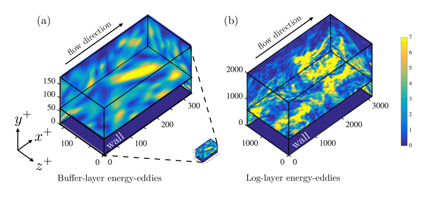
The most celebrated conceptual model for wall-bounded turbulence was proposed by Townsend (1976), who envisioned the flow as a multiscale population of energy/momentum-eddies starting from the wall and spanning a wide range of sizes across the boundary layer thickness as highlighted in figure 1. The conceptualisation of the flow as a superposition of energy-eddies of different sizes is usually referred to as the wall-attached eddy model. The smallest energy-eddies are located closer to the wall, in the buffer layer, and their sizes are dictated by the limiting effect of the fluid viscosity. For example, the size of the buffer layer energy-eddies may be of the order of millimetres for atmospheric flows (Marusic et al., 2010). Further from the wall, in the so-called logarithmic layer (log layer), the flow is also organised into energy-eddies that differ from those in the buffer layer by their larger dimensions, e.g., of the order of hundreds of meters for atmospheric flows (Marusic et al., 2010).

Figure 1: Instantaneous turbulence kinetic energy, $(u^{\prime 2}+v^{\prime 2}+w^{\prime 2})/2$, where the prime denotes fluctuating quantities with respect to their mean values defined by averaging in the homogeneous directions and time. The turbulence kinetic energy is normalised in wall units and plotted for planes parallel to streamwise and wall-normal directions. The data is from a DNS of a turbulent channel flow at $Re_{\tau}\approx 4200$ in a non-minimal domain by Lozano-Durán & Jiménez (2014a). The red ovals highlight the location of energy-eddies of different sizes in the buffer and log layers, respectively, while the white dashed lines indicate the local domain of each eddy.

The existence of wall-attached energy-eddies as depicted above is endorsed by a growing number of studies. The footprint of attached flow motions has been observed experimentally and numerically in the spectra and correlations at relatively modest Reynolds numbers in pipes (Morrison & Kronauer, 1969; Perry & Abell, 1975, 1977; Bullock et al., 1978; Kim, 1999; Guala et al., 2006; McKeon et al., 2004; Bailey et al., 2008; Hultmark et al., 2012) and in turbulent channels and flat-plate boundary layers (Tomkins & Adrian, 2003; Del Alamo et al., 2004; Hoyas & Jiménez, 2006; Monty et al., 2007; Hoyas & Jiménez, 2008; Vallikivi et al., 2015; Chandran et al., 2017). Other works have extended the attached-eddy model (Perry & Chong, 1982; Perry et al., 1986; Perry & Marusic, 1995) or complemented the original picture proposed by Townsend (Mizuno & Jiménez, 2011; Davidson et al., 2006; Dong et al., 2017; Lozano-Durán & Bae, 2019). Reviews of the Townsend’s model can be found in Smits et al. (2011), Jiménez (2012, 2013, 2018) and Marusic & Monty (2019).

Traditionally, wall-attached eddies have been interpreted as statistical entities (Marusic et al., 2010; Smits et al., 2011), but recent works suggest that they can also be identified as instantaneous features of the flow (see Jiménez, 2018, and references therein). The methodologies to identify instantaneous energy-eddies are diverse and frequently complementary, ranging from the Fourier characterisation of the turbulent kinetic energy (Jiménez, 2013, 2015) to adaptive mode decomposition (Hellström et al., 2016; Cheng et al., 2019; Agostini & Leschziner, 2019), and three-dimensional clustering techniques (e.g. Del Álamo et al., 2006; Lozano-Durán et al., 2012; Lozano-Durán & Jiménez, 2014b; Hwang & Sung, 2018, 2019), to name a few. The detection and isolation of energy-eddies have deepened our understanding of the spatial structure of turbulence. However, the most interesting results are not the kinematic description of these eddies in individual flow realisations, but rather the elucidation of how they relate to each other and, more importantly, how they evolve in time.

In the buffer layer, the current consensus is that energy-eddies are involved in a temporal self-sustaining cycle (Jiménez & Moin, 1991; Hamilton et al., 1995; Waleffe, 1997; Schoppa & Hussain, 2002; Farrell et al., 2017) based on the emergence of streaks from wall-normal ejections of fluid (Landahl & Landahlt, 1975) followed by the meandering and breakdown of the newborn streaks (Swearingen & Blackwelder, 1987; Waleffe, 1995, 1997; Kawahara et al., 2003). The cycle is restarted by the generation of new vortices from the perturbations created by the disrupted streaks. In this framework, it is hypothesised that streamwise vortices collect the fluid from the inner region, where the flow is very slow, and organise it into streaks (cf. Butler & Farrell, 1993). Other works suggest that the generation of streaks are due to the structure-forming properties of the linearised Navier–Stokes operator, independently of any organised vortices (Chernyshenko & Baig, 2005). Conversely, the streaks are hypothesised to trigger the formation of vortices by losing their stability (Waleffe, 1997; Farrell & Ioannou, 2012) or the collapse of vortex sheets via streamwise stretching (Schoppa & Hussain, 2002). The reader is referred to Panton (2001) and Jiménez (2018) for reviews on self-sustaining processes in the buffer layer.

A similar but more disorganised scenario is hypothesised to occur for the larger wall-attached energy-eddies within the log layer (Flores & Jiménez, 2010; Hwang & Cossu, 2011; Cossu & Hwang, 2017). The existence of a self-similar streak/roll structure in the log layer consistent with Townsend’s attached-eddy model has been supported by the numerical studies by Del Álamo et al. (2006); Flores & Jiménez (2010); Hwang & Cossu (2011); Lozano-Durán et al. (2012) and Lozano-Durán & Jiménez (2014b), among others. A growing body of evidence also indicates that the generation of the log-layer streaks has its origins in the linear lift-up effect (Kim & Lim, 2000; Del Álamo & Jiménez, 2006; Pujals et al., 2009; Hwang & Cossu, 2010; Moarref et al., 2013; Alizard, 2015) in conjunction with the Orr’s mechanism (Orr, 1907; Jiménez, 2012). Regarding roll formation, several works have speculated that they are the consequence of a sinuous secondary instability of the streaks that collapse through a rapid meander until breakdown (Andersson et al., 2001; Park et al., 2011; Alizard, 2015; Cassinelli et al., 2017), while others advocate for a parametric instability of the streamwise-averaged mean flow as the generating mechanism of the rolls (Farrell et al., 2016).

Although it is agreed that both the buffer-layer and log-layer energy-eddies are involved in a self-sustaining cycle, their causal relationships have only been assessed indirectly by altering the governing equations of fluid motion (Jiménez & Pinelli, 1999; Hwang & Cossu, 2010, 2011; Farrell et al., 2017). Moreover, the mechanisms discussed above, each capable of leading to the observed turbulence structure, are rooted in simplified theories or conceptual arguments. Whether the flow follows any or a combination of these mechanisms is in fact unclear. Most interpretations stem from linear stability theory, which has proved successful in providing a theoretical framework to rationalise the length and time scales observed in the flow (Pujals et al., 2009; Del Álamo & Jiménez, 2006; Jiménez, 2015). However, a base flow must be selected a priori to enable the linearisation of the equations, which introduces an important degree of arbitrariness, and quantitative results are known to be sensitive to the details of the base state (Vaughan & Zaki, 2011; Lozano-Durán et al., 2018b). Another criticism for linear theories comes from the fact that turbulence is a highly nonlinear phenomenon, and a complete self-sustaining cycle cannot be anticipated from a single set of linearised equations.

The limitations above have hampered the comparison of the flow dynamics in the buffer and log layers, and there is no conclusive evidence on whether the mechanisms controlling the eddies at different scales are of similar nature. One major obstacle arises from the lack of a tool in turbulence research that resolves the cause-and-effect dilemma and unambiguously attributes a set of observed dynamics to well-defined causes. This brings to attention the issue of causal inference, which is a central theme in many scientific disciplines but has barely been discussed in turbulent flows with the exception of a handful of works (Cerbus & Goldburg, 2013; Tissot et al., 2014; Liang & Lozano-Durán, 2017; Bae et al., 2018a). Given that the events in question are usually known in the form of time series, the quantification of causality among temporal signals has received the most attention. Typically, causal inference is simplified in terms of time-correlation between pairs of signals. However, it is known that correlation lacks the directionality and asymmetry required to guarantee causation (Beebee et al., 2012). To overcome the pitfalls of correlations, Granger (1969) introduced a widespread test for causality assessment based on the statistical usefulness of a given time signal in forecasting another. Nonetheless, there are ongoing concerns regarding the presumptions about the joint statistical distribution of the data as well as the applicability of Granger causality to strongly nonlinear systems (Stokes & Purdon, 2017). In an attempt to remedy this deficiency, recent works have centred their attention to information-theoretic measures of causality such as transfer entropy (Schreiber, 2000) and information flow (Liang & Kleeman, 2006; Liang, 2014). The former is notoriously challenging to evaluate, requiring long time series and high associated computation cost (Hlavackova-Schindler et al., 2007), but recent advancements in entropy estimation from insufficient datasets (Kozachenko & Leonenko, 1987; Kraskov et al., 2004) and the advent of longer time-series from numerical simulations have made transfer entropy a viable approach.

In this study, we use transfer entropy from information theory to quantify the causality among energy-eddies. Our goal is to compare the fully nonlinear self-sustaining processes in the buffer layer and log layer with minimum intrusion. We show that eddies in both layers follow comparable self-sustaining processes despite their vastly different sizes. Our findings are also used to inspect the implications of self-similar causality of energy-eddies for the control and modelling of wall turbulence.

The paper is organised as follows. The numerical experiments and methods are introduced in §2. In §2.1, we describe two numerical simulations to isolate the energy-eddies in the buffer layer and log layer, respectively. The characterisation of energy-eddies as time signals is discussed in §2.2, and the methodology for quantifying causal interactions among the signals is offered in §2.3. The results are presented in §3. We first investigate the relevant time-scales for causal inference in §3.1, then the causal links among energy-eddies in §3.2, and finally some applications to flow modelling in §3.3. We conclude our study in §4.

2 Numerical experiments and methods

2.1 Isolating energy-eddies at different scales

To investigate the self-sustaining process of the energy-eddies at different scales, we examine data from two temporally resolved DNS of an incompressible turbulent channel flow. Each simulation is performed within a computational domain tailored to isolate just a few of the most energetic eddies in either the buffer layer (Jiménez & Moin, 1991) or log layer (Flores & Jiménez, 2010), respectively, and can be considered as the simplest numerical set-up to study wall-bounded energy-eddies of a given size. The configuration of the two simulations is illustrated in figures 2(a) and (b) (see also Movie 1).

Figure 2: Minimal simulations of wall-bounded turbulence to isolate energy-eddies in (a) the buffer layer, and (b) the log layer. The quantity represented is the turbulence kinetic energy at different planes. Only half of the channel domain is shown in the $y$-direction. The wall is located at $y^{+}=0$, quantities are scaled in $+$ units, and the arrows indicate the mean flow direction. Panel (a) also includes the computational domain for the buffer-layer simulation, shown at scale with respect to the log-layer simulation in panel (b). See also Movie 1.

Hereafter, the streamwise, wall-normal, and spanwise directions are denoted by $x$, $y$, and $z$, respectively, and the corresponding flow velocity components by $u$, $v$, and $w$. Each DNS is characterised by its friction Reynolds number $\mathrm{Re}_{\tau}=\delta/\delta_{v}$, where $\delta$ is the channel half-height and $\delta_{v}$ is the viscous length scale defined in terms of the kinematic viscosity of the fluid, $\nu$, and the friction velocity at the wall, $u_{\tau}$. Our friction Reynolds numbers are $\mathrm{Re}_{\tau}\approx 180$ for the buffer-layer simulation and $\mathrm{Re}_{\tau}\approx 2000$ for the log layer case, which yield a scale separation of roughly a decade between the energy-eddies in each simulation. The disparity in sizes between the buffer and log layers DNS domains is remarked in figure 2. Lengths and velocities normalised by $\delta_{v}$ and $u_{\tau}$, respectively, are denoted by the superscript $+$.

For the buffer-layer simulation, the streamwise, wall-normal, and spanwise domain sizes are $L_{x}^{+}\approx 337$, $L_{y}^{+}\approx 368$ and $L_{z}^{+}\approx 168$, respectively. Jiménez & Moin (1991) showed that simulations in this domain constitute an elemental structural unit containing a single streamwise streak and a pair of staggered quasi-streamwise vortices, which reproduce reasonably well the statistics of the flow in larger domains. For the log-layer simulation, the length, height, and width of the computational domain are $L_{x}^{+}\approx 3148$, $L_{y}^{+}\approx 4008$ and $L_{z}^{+}\approx 1574$, respectively. These dimensions correspond to a minimal box simulation for the log layer and are considered to be sufficient to isolate the relevant dynamical structures involved in the bursting process (Flores & Jiménez, 2010). Minimal log-layer simulations have also demonstrated their ability to reproduce statistics of full-size turbulence computed in larger domains (Jiménez, 2012).

The flow is simulated for more than $800\delta/u_{\tau}$ after transients. This period of time is orders of magnitude longer than the typical lifetime of the individual energy-eddies in the flow, whose lifespans are statistically shorter than $\delta/u_{\tau}$ (Lozano-Durán & Jiménez, 2014b). During the simulation, snapshots of the flow were stored frequently in time every $0.03\delta/u_{\tau}$ ($\approx$$5\delta_{v}/u_{\tau}$) and $0.05\delta/u_{\tau}$ ($\approx$$90\delta_{v}/u_{\tau}$) for the buffer and log layers, respectively. It is also convenient to normalise the values above with the time-scale introduced by mean shear $S^{-1}$, defined by averaging in the homogeneous directions, time, and a prescribed band along the wall-normal direction. Selecting as representative bands $y^{+}\in[40,80]$ and $y^{+}\in[500,700]$ for the buffer layer and log layer, respectively (more details in §2.2), our simulations span a period longer than $10^{3}S^{-1}$, with a time-lag between stored snapshots smaller than $0.5S^{-1}$. The long yet temporally resolved datasets of the current study enable the statistical characterisation of many eddies throughout their entire life cycle.

The simulations are performed by discretising the incompressible Navier-Stokes equations with a staggered, second-order accurate, central finite difference method in space (Orlandi, 2000), and a explicit third-order accurate Runge-Kutta method (Wray, 1990) for time advancement. The system of equations is solved via an operator splitting approach (Chorin, 1968). Periodic boundary conditions are imposed in the streamwise and spanwise directions, and the no-slip condition is applied at the walls. The flow is driven by a constant mean pressure gradient in the streamwise direction. For both the buffer and log layers, the streamwise and spanwise grid resolutions are uniform and equal to $\Delta x^{+}\approx 6$, and $\Delta z^{+}\approx 3$, respectively. The wall-normal grid resolution, $\Delta y$, is stretched in the wall-normal direction following an hyperbolic tangent with $\Delta y_{\min}^{+}\approx 0.3$ and $\Delta y_{\max}^{+}\approx 10$. The time step is such that the Courant-Friedrichs-Lewy condition is always below 0.5 during the run. The code has been validated in turbulent channel flows (Bae et al., 2018c, b) and flat-plate boundary layers (Lozano-Durán et al., 2018a). Details on the parameters of the numerical set-up are included in table 1.

Simulation	$Re_{\tau}$	$L_{x}^{+}$	$L_{z}^{+}$	$\Delta x^{+}$	$\Delta z^{+}$	$\Delta y_{\min}^{+}$	$\Delta y_{\max}^{+}$	$N_{x}$	$N_{y}$	$N_{z}$	$Tu_{\tau}/\delta$	$1/S^{+}$
Buffer layer	184	337	168	5.3	2.6	0.2	7.2	32	129	32	830	24
Log layer	2004	3148	1574	6.1	3.1	0.3	13.1	512	769	512	801	212

Table 1: Geometry and parameters of the simulations. $Re_{\tau}$ is the friction Reynolds number. $L_{x}^{+}$ and $L_{z}^{+}$ are the streamwise and spanwise dimensions of the numerical box in wall units, respectively. $\Delta x^{+}$ and $\Delta z^{+}$ are the spatial grid resolutions for the streamwise and spanwise direction, respectively. $\Delta y_{\min}^{+}$ and $\Delta y_{\max}^{+}$ are the finer (closer to the wall) and coarser (further from the wall) grid resolutions in the wall-normal direction. $N_{x}$, $N_{y}$, and $N_{z}$ are the number of streamwise, wall-normal, and spanwise grid points, respectively. The simulations are integrated for a time $Tu_{\tau}/\delta$, where $u_{\tau}$ is the friction velocity and $\delta$ is the channel half-height. $S$ is the mean shear within the wall-normal bands $y^{+}\in[40,80]$ and $y^{+}\in[500,700]$ for the buffer layer and log layer, respectively, and $1/S^{+}$ defines a characteristic time-scale for each layer.

2.2 Characterisation of energy-eddies as time signals

The next step is to quantify the kinetic energy carried by the streaks and rolls as a function of time. To do that, we use the Fourier decomposition, $\check{(\cdot)}$, of each velocity component in the streamwise and spanwise directions (Onsager, 1949), i.e., $\check{u}_{n,m}(y,t)$, $\check{v}_{n,m}(y,t)$, and $\check{w}_{n,m}(y,t)$, where the streamwise ($n$) and spanwise ($m$) wavenumbers are normalised such that $n=1$ ($m=1$) represents one streamwise (spanwise) period of the domain. The velocities are first averaged in bands along the wall-normal direction to produce Fourier components (or modes) that do not depend on $y$, e.g.,

$$\hat{u}_{n,m}(t)=\frac{1}{y_{1}-y_{0}}\int_{y_{0}}^{y_{1}}\check{u}_{n,m}(y,t)\mathrm{d}y,$$ (1)

and similarly for $\hat{v}_{n,m}(t)$ and $\hat{w}_{n,m}(t)$. The bands selected are $(y_{0}^{+},y_{1}^{+})=(40,80)$ for the buffer layer and $(y_{0}^{+},y_{1}^{+})=(500,700)$ for the log layer. These bands are chosen consistently with the regions of realistic turbulence reported for minimal boxes in the buffer layer (Jiménez & Moin, 1991) and the log layer (Flores & Jiménez, 2010). It was tested that the results presented here are qualitatively similar for $y_{0}^{+}$ and $y_{1}^{+}$ within the range $[20,100]$ and $[300,900]$ for the buffer and log layers, respectively.

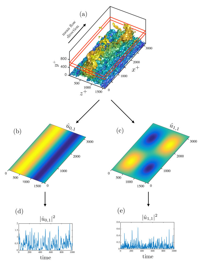
The process of decomposing $u$ (similarly for $v$ and $w$) into time signals for the log layer (similarly for the buffer layer) is schematically summarised in figure 3: the instantaneous $u$ (figure 3a) is transformed into the wall-normal averaged Fourier modes $\hat{u}_{0,1}$ and $\hat{u}_{1,1}$, whose spatial structure is shown in figures 3(b) and (c), respectively. Then, the kinetic energy associated with each mode, namely, $|\hat{u}_{0,1}|^{2}$ and $|\hat{u}_{1,1}|^{2}$, is obtained as a function of time as shown in figure 3(d) and (e). In this manner, $|\hat{u}_{0,1}|^{2}$ characterises the evolution of the kinetic energy of straight streaks, while meandering or broken streaks are represented by $|\hat{u}_{1,1}|^{2}$. Analogously, rolls identified by $|\hat{v}_{n,m}|^{2}$ and $|\hat{w}_{n,m}|^{2}$ are divided into long motions ($|\hat{v}_{0,1}|^{2}$ and $|\hat{w}_{1,0}|^{2}$) and short motions ($|\hat{v}_{1,1}|^{2}$ and $|\hat{w}_{1,1}|^{2}$). The resulting set of signals can be arranged into a six-component vector (one per layer) defined by

$$\boldsymbol{\mathcal{V}}(t)=[\mathcal{V}_{1},\mathcal{V}_{2},...,\mathcal{V}_{6}]=\left[|\hat{u}_{0,1}|^{2},|\hat{v}_{0,1}|^{2},|\hat{w}_{1,0}|^{2},|\hat{u}_{1,1}|^{2},|\hat{v}_{1,1}|^{2},|\hat{w}_{1,1}|^{2}\right].$$ (2)

The vector $\boldsymbol{\mathcal{V}}(t)$ characterises the spatial and temporal evolution of energy-eddies, and all together account for roughly 50% of the total kinetic energy of the flow within the wall-normal band considered in both layers.

Figure 3: Characterisation of energy-eddies as time signals. (a) Isosurface of the instantaneous streamwise velocity in the log layer. The value of the isosurface is 0.7 of the maximum streamwise velocity, coloured by the distance to the wall from dark blue (close to the wall) to light yellow (far from the wall). The red lines delimit the wall-normal region where $u$ is averaged. Panels (b) and (c) show the spatial structure of the Fourier modes associated with $\hat{u}_{0,1}$ and $\hat{u}_{1,1}$, respectively. Panels (d) and (e) are the time evolution of $|\hat{u}_{0,1}|^{2}$ and $|\hat{u}_{1,1}|^{2}$ in the log layer. Time is normalised with the mean shear across the band considered for extracting the time signals, and the velocities are scaled in $+$ units.

2.3 Causality among time-signals as transfer entropy

We use the framework provided by information theory (Shannon, 1948) to quantify causality among time-signals. The central quantity for causal assessment is the Shannon entropy (or uncertainty) of the signals, which is intimately related to the arrow of time (Eddington, 1929). The connection between the entropy and the arrow of time is argued by the fact that the laws of physics are time-symmetric at the microscopic level, and it is only from the macroscopic viewpoint that time-asymmetries arise in the system. Such asymmetries can be statistically measured using information-theoretic metrics based on the Shannon entropy. Within this framework, causality from a $\mathcal{V}_{j}$ to $\mathcal{V}_{i}$ is defined as the decrease in uncertainty of $\mathcal{V}_{i}$ by knowing the past state of $\mathcal{V}_{j}$. The method exploits the principle of time-asymmetry of causation (causes precede the effects) and is mathematically formulated through the transfer entropy (Schreiber, 2000). Considering the vector $\boldsymbol{\mathcal{V}}(t)$ as defined in (2), the transfer entropy (or causality) from $\mathcal{V}_{j}$ to $\mathcal{V}_{i}$ is defined as (Schreiber, 2000; Duan et al., 2013)

$$T_{j\rightarrow i}(\Delta t)=H(\mathcal{V}_{i}(t)|\boldsymbol{\mathcal{V}}^{\bcancel{j}}(t-\Delta t))-H(\mathcal{V}_{i}(t)|\boldsymbol{\mathcal{V}}(t-\Delta t)),$$ (3)

where $T_{j\rightarrow i}$ is the causality from $\mathcal{V}_{j}$ to $\mathcal{V}_{i}$, $\Delta t$ is the time-lag to evaluate causality, $H(\mathcal{V}_{i}|\boldsymbol{\mathcal{V}})$ is the conditional Shannon entropy (Shannon, 1948) (i.e., the uncertainty in a variable $\mathcal{V}_{i}$ given $\boldsymbol{\mathcal{V}}$), and $\boldsymbol{\mathcal{V}}^{\bcancel{j}}$ is equivalent to $\boldsymbol{\mathcal{V}}$ but excluding the component $j$. The conditional Shannon entropy of a variable $\mathcal{V}_{i}$ given $\boldsymbol{\mathcal{V}}$ is defined as

$$H(\mathcal{V}_{i}|\boldsymbol{\mathcal{V}})=E[\log(f(\mathcal{V}_{i},\boldsymbol{\mathcal{V}}))]-E[\log(f(\boldsymbol{\mathcal{V}}))],$$ (4)

where $f(\cdot)$ is the probability density function, and $E[\cdot]$ signifies the expected value.

We are concerned with the cross-induced causalities $T_{j\rightarrow i}$, with $j\neq i$, hence, $T_{i\rightarrow i}$ are set to zero. Moreover, our goal is to evaluate the causal effect of $T_{j\rightarrow i}$ relative to the total causality from $\mathcal{V}_{j}$ to all the variables. Thus, we define the normalised causality as

$$\tilde{T}_{j\rightarrow i}(\Delta t)=\frac{T_{j\rightarrow i}(\Delta t)-T_{j\rightarrow i}^{\mathrm{perm}}(\Delta t)}{T_{j\rightarrow(1,\cdots,6)}(\Delta t)-T_{j\rightarrow(1,\cdots,6)}^{\mathrm{perm}}},$$ (5)

such that the value of $\tilde{T}_{j\rightarrow i}$ is bounded between 0 and 1. The term $T_{j\rightarrow i}^{\mathrm{perm}}$ aims to remove spurious contributions due to statistical errors, and it is the transfer entropy computed from the variables $\mathcal{V}_{1},\cdots,\mathcal{V}_{j-1},\mathcal{V}_{j}^{\mathrm{perm}},\mathcal{V}_{j+1},\cdots,\mathcal{V}_{6}$, where $\mathcal{V}_{j}^{\mathrm{perm}}$ is $\mathcal{V}_{j}$ randomly permuted in time in order to preserve the one-point statistics of the signal while breaking time-delayed causal links. The calculation of (5) is numerical performed by estimating the probability density functions and their corresponding entropy using the binning method. More details about the computation of $T_{j\rightarrow i}$ are given in appendix A.

There is a growing recognition that information-theoretic metrics such as transfer entropy are fundamental physical quantities enabling causal inference from observational data (Prokopenko & Lizier, 2014; Spinney et al., 2016). Moreover, causality measured by (5) is advantageous compared to classic time-correlations employed in previous studies of wall turbulence (Jiménez, 2013). One desirable property is the asymmetry of the measurement, i.e., if a variable $\mathcal{V}_{i}$ is causal to $\mathcal{V}_{j}$, it does not imply that $\mathcal{V}_{j}$ is causal to $\mathcal{V}_{i}$. Another attractive feature of transfer entropy is that it is based on probability density functions and, hence, is invariant under shifting, rescaling and, in general, under nonlinear transformations of the signals (Kaiser & Schreiber, 2002). Additionally, $T_{j\rightarrow i}$ accounts for direct causality excluding intermediate variables: if $\mathcal{V}_{i}$ is only caused by $\mathcal{V}_{j}$ and $\mathcal{V}_{k}$ is only caused by $\mathcal{V}_{j}$, there is no causality from $\mathcal{V}_{i}$ to $\mathcal{V}_{k}$ provided that the three components are contained in $\boldsymbol{\mathcal{V}}$ (Duan et al., 2013).

Finally, we close the section noting that the quest of identifying cause-effect relationships among events or variables remains an open challenge in scientific research. Formally, the transfer entropy in (3) determines the statistical direction of information transfer between time-signals by measuring asymmetries in their interactions. We have adopted this metric as an indication of causality, but the definition of causation is subject to ongoing debate and controversy. Although transfer entropy entails a quantitative improvement with respect to other methodologies for causal inference, it is not flawless. Previous works have reported that transfer entropy obtained from poor time-resolved datasets or short time sequences are prone to yield biased estimates (Hahs & Pethel, 2011). More importantly, if some variables in the system are unavailable or neglected, or if the time-lag in consideration does not account for the actual causal time-lag of the signals, this could have profound consequences in the observed causality due to intermediate or confounding hidden variables. The reader is referred to Hlavackova-Schindler et al. (2007) for an in-depth discussion on information theory in causal inference.

3 Results

3.1 Time-scales for causal inference

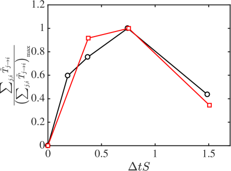
Assessing causality in (5) requires the identification of a characteristic time-lag, $\Delta t$. In the present study, we seek $\Delta t$ for maximum causal inference, $\Delta t_{\max}$. The behaviour of $\tilde{T}_{j\rightarrow i}(\Delta t)$ can differ for each $(j,i)$ pair, but a sensible choice to estimate $\Delta t_{\max}$ is obtained by defining a global measure based on the summation of all causalities for each $\Delta t$, i.e., $\sum_{j,i}\tilde{T}_{j\rightarrow i}$. The results are shown in figure 4, where $\Delta t$ is scaled by the average shear within the bands considered for each layer.

Interestingly, causalities for both the buffer layer and log layer peak at $\Delta t_{\max}\approx 0.8S^{-1}$, which is the time-lag selected for the remainder of the study. Note that from table 1, the ratio $S_{\mathrm{buffer}}/S_{\mathrm{log}}$ is roughly 10, and there is a non-trivial time-scale separation between both layers. The value of $\Delta t_{\max}$ is comparable to the characteristic lifespan of coherence structures and the duration of bursting events in turbulent channel flows (Flores & Jiménez, 2010; Lozano-Durán & Jiménez, 2014b; Jiménez, 2018). Moreover, the collapse in figure 4 of the causal time-horizon for both layers in shear times points at $S^{-1}$ as the physically relevant time-scale controlling the energy-eddies (Mizuno & Jiménez, 2011; Lozano-Durán & Bae, 2019). The result is also consistent with previous works on self-sustaining processes, which have shown that shear turbulence behaves quasi-periodically with time cycles proportional to $S^{-1}$ (Sekimoto et al., 2016).

Figure 4: Summation of causalities $\sum_{j,i}\tilde{T}_{j\rightarrow i}$ as a function of the time horizon for causal influence, $\Delta t$, for the buffer layer (black circles) and log layer (red squares). $\Delta t$ is scaled by the average shear of each layer, and causalities in the vertical axis are normalised by the maximum value among all $\Delta t$.

3.2 Causal structure of wall-bounded energy-eddies

The key result of this work is shown in figure 5, which contains the causal relations $\tilde{T}_{j\rightarrow i}$ among the six flow components. Figure 5 is divided into two causal maps, one for each layer. The maps should be read as causative variables in the horizontal axis versus the corresponding effects in the vertical axis. The resemblance between the maps reveals that, despite the complex nonlinear dynamics and the sizeable length- and time-scale difference between buffer-layer and log-layer energy-eddies, there is a strikingly similar causal pattern shared among energy signals in both layers.

The causal maps in figure 5 also unify several well-known flow mechanisms in a single visual. If we separate the maps into two subsets, namely, intra-scale causalities (red squares in figure 5), and inter-scale causalities (black squares in figure 5), the strongest causalities occur among velocity signals at the same scale. The causal connections $|\hat{v}_{1,1}|^{2}\rightarrow|\hat{u}_{1,1}|^{2}$ and $|\hat{v}_{0,1}|^{2}\rightarrow|\hat{u}_{0,1}|^{2}$ are consistent with the wall-normal momentum transport by $v$, which intensifies the streak amplitude through the Orr/lift-up mechanism (Orr, 1907; Landahl & Landahlt, 1975). During this process, the causality $|\hat{v}_{1,1}|^{2}\rightarrow|\hat{w}_{1,1}|^{2}$ is anticipated by the formation of streamwise rolls enforced by the incompressibility of the flow. The most notable inter-scale causal links arise from $|\hat{u}_{1,1}|^{2}\rightarrow|\hat{w}_{1,0}|^{2}$, and $|\hat{w}_{1,0}|^{2}\rightarrow|\hat{v}_{1,1}|^{2}$. The former is reminiscent of the spanwise flow motions induced by the loss of stability of the streaks, while the latter is consistent with the subsequent meander and breakdown (Swearingen & Blackwelder, 1987; Waleffe, 1995, 1997; Kawahara et al., 2003; Park et al., 2011; Alizard, 2015; Cassinelli et al., 2017). In contrast with previous studies, our results stem directly from the non-intrusive analysis of the fully non-linear signals and do not rely on a particular linearisation of the equations of motion. Yet, linear theories and causal analysis do not oppose to each other and they should be perceived as complementary approaches; the former as a reduced system to investigate different flow mechanisms, and the latter as a mean to assess whether those processes are consistent with the time-evolution of the actual non-linear flow.

Figure 5: Causal maps for (a) buffer layer and (b) log layer. Greyscale colours denote normalised causality magnitude. The variables $|\hat{u}_{n,m}|^{2}$, $|\hat{v}_{n,m}|^{2}$, and $|\hat{w}_{n,m}|^{2}$ represent the magnitudes of the streamwise, wall-normal, and spanwise velocity modes, respectively. Red and blue squares enclose intra-scale causalities and inter-scale causalities, respectively. The statistical convergence of the causal maps is assessed in appendix B.

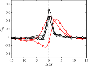
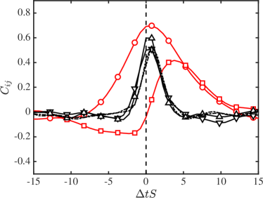
For completeness, we also discuss the time cross-correlation between fluctuating signals $\mathcal{V}^{\prime}_{i}=\mathcal{V}_{i}-\langle\mathcal{V}_{i}\rangle_{t}$ calculated as

$$C_{ij}(\Delta t)=\frac{\langle\mathcal{V}^{\prime}_{i}(t)\mathcal{V}^{\prime}_{j}(t+\Delta t)\rangle_{t}}{\langle\mathcal{V}^{\prime 2}_{i}(t)\rangle_{t}^{1/2}\langle\mathcal{V}^{\prime 2}_{j}(t)\rangle_{t}^{1/2}},$$ (6)

where the average $\langle\cdot\rangle_{t}$ is taken over whole time history. The results are displayed in figure 6, which includes correlations whose maxima are above 0.4. Both the buffer and log layers exhibit similar trends in the correlations, consistent with the self-similar causality shown above. Here, we wish to make qualitative comparisons of $C_{ij}$ with the maps in figure 5, and the reader is referred to Jiménez (2013) for a further discussion on time-correlations in minimal channel flows.

An immediate consequence of causality is the emergence of some degree of correlation between variables, although the converse is not necessarily true. Despite this footprint of causality onto the correlations, fair comparisons of $C_{ij}$ and $T_{i\rightarrow j}$ are hindered by the intrinsic differences of each methodology. As discussed in §2.3, the temporal symmetry of the correlations, $C_{ij}(\Delta t)=C_{ji}(-\Delta t)$, does not enable the unidirectional assessment of interactions between variables. To overcome this limitation and only for the sake of qualitative comparisons, we assume that the amount of “causality” from $\mathcal{V}_{i}$ to $\mathcal{V}_{j}$ can be inferred from the skewness of $C_{ij}$ towards later times. Adopting this convention, the prevailing directionalities in the correlations are identified as $|\hat{u}_{i,j}|^{2}\rightarrow(|\hat{v}_{i,j}|^{2},|\hat{w}_{j,i}|^{2})$ and $|\hat{v}_{1,1}|^{2}\rightarrow|\hat{w}_{1,1}|^{2}$, which are also recognised in the causal maps in figure 5. The picture provided above is that the correlations are mostly dominated by strong events associated with the redistribution of energy from the streamwise velocity component to the cross-flow (Mansour et al., 1988). However, $C_{ij}$ fails to account for key mechanisms required for sustaining wall turbulence, such as the lift-up/Orr effect (Kim & Lim, 2000), which is vividly captured by the causal maps. Regarding the time-scales, the peaks of the time-correlations are attained within the range $\Delta t\approx 0S^{-1}$ to $\Delta t\approx 3S^{-1}$. The range encloses the averaged time-horizon for maximum causal inference $\Delta t_{\max}\approx S^{-1}$ (§3.1), and both approaches appear as valid to extract the representative time-scales of the flow. Overall, the inference of causality based on the skewness of $C_{ij}$ is obscured by the often mild asymmetries in $C_{ij}$ and the bias towards strong events, whereas the causal maps in figure 5 convey a richer vision of the flow mechanisms easing the limitations of $C_{ij}$.

(a)

(b)

Figure 6: Temporal cross-correlation of $|\hat{u}_{0,1}|^{2}\rightarrow|\hat{v}_{0,1}|^{2}$, $\circ$; $|\hat{u}_{0,1}|^{2}\rightarrow|\hat{w}_{1,0}|^{2}$, $\square$; $|\hat{u}_{1,1}|^{2}\rightarrow|\hat{v}_{1,1}|^{2}$, $\triangledown$; $|\hat{u}_{1,1}|^{2}\rightarrow|\hat{w}_{1,1}|^{2}$, $\triangle$; $|\hat{v}_{1,1}|^{2}\rightarrow|\hat{w}_{1,1}|^{2}$,            . The vertical dashed line is $\Delta t=0S^{-1}$. (a) buffer layer. (b) Log layer. The notation used is such that $C_{ij}$ represents $\mathcal{V}_{i}\rightarrow\mathcal{V}_{j}$. Lines in black are used for weakly skewed $C_{ij}$. Time is scaled with the shear averaged over the respective bands.

3.3 Application to flow modelling: bursts prediction in the log layer

The observation of similar causality of energy-eddies at different scales in wall turbulence has striking implications for control and modelling. Our goal in this section is to provide a simple demonstration of how new models can be conceived for the computationally affordable smaller eddies in the buffer layer, to later model eddies at larger scales. This is shown by constructing a model to predict $|\hat{v}_{1,1}|^{2}$ in the log layer using information from buffer layer simulations. Other quantities in $\boldsymbol{\mathcal{V}}$ are equally amenable to modelling, and the choice of $|\hat{v}_{1,1}|^{2}$ constitutes just one possibility. The selection of $|\hat{v}_{1,1}|^{2}$ can be motivated as a marker of the bursting phenomena observed in intense wind gusts relevant for buildings and aircraft structural loads (Fujita, 1981).

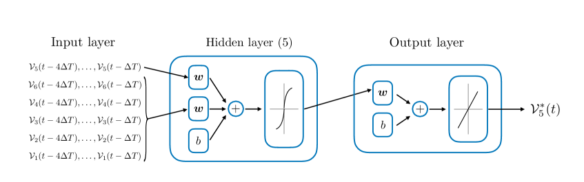
We model $\mathcal{V}_{5}=|\hat{v}_{1,1}|^{2}$ at time $t$ using a nonlinear autoregressive exogenous neural network (NN) (McCulloch & Pitts, 1943). The modelling approach is justified by the suitability of NN for time-signal forecasting in nonlinear systems, but the remainder of the section could have been formulated using traditional linear models without altering our conclusions. Our NN model relates the current value of a time series ($\mathcal{V}_{5}$) to both past values of the same series and current and past values of the driving (exogenous) series ($\mathcal{V}_{i},\ i=1,\dots,6,\ i\neq 5$). Figure 7 shows an schematic of the NN set-up. The input of the network is the known past states of the log-layer signals $\boldsymbol{\mathcal{V}}$ at times $t-\Delta t,...,t-4\Delta t$, with $\Delta t=0.8S^{-1}$. In present model, $\mathcal{V}_{5}=|\hat{v}_{1,1}|^{2}$ at time $t$ is estimated as

$$\mathcal{V}_{5}^{*}(t)=F\left(\boldsymbol{\mathcal{V}}(t-\Delta T),\boldsymbol{\mathcal{V}}(t-2\Delta T),\boldsymbol{\mathcal{V}}(t-3\Delta T),\boldsymbol{\mathcal{V}}(t-4\Delta T)\right)+\epsilon(t),$$ (7)

where the function $F$ is a five-layers recursive neural network as detailed in figure 7, $\mathcal{V}_{5}^{*}(t)$ is a prediction of $\mathcal{V}_{5}(t)$, $\Delta T$ is the time-lag, and $\epsilon$ is the model error. The activation function selected for the hidden layers is the hyperbolic tangent sigmoid transfer function. The NN is trained using Bayesian regularisation backpropagation with five hidden layers. The training data is divided randomly into two groups, the training (80%) and validation (20%) sets. The training is terminated when the damping factor of the Levenberg-Marquardt algorithm exceeds $10^{10}$. Additional details about the NN can be found in Lin et al. (1996) and Gao & Er (2005).

Figure 7: Schematics of the nonlinear autoregressive exogenous neural network. The input layer comprises the variables $\boldsymbol{\mathcal{V}}$ at past the times $t-\Delta T$, $t-2\Delta T$, $t-3\Delta T$, and $t-4\Delta T$. The five hidden layers consist of weights ($\boldsymbol{w}$) and bias ($b$). The output layer returns an estimation at time $t$ of the variable of interest $\mathcal{V}_{5}^{*}=|\hat{v}^{*}_{1,1}|^{2}$.

Three datasets are considered to train the NN prior to performing the predictions shown in figure 8:

• In the first case, the NN is trained using signals from the log layer that are independent of the dataset we aim to predict. Next, the NN is used to make one step predictions of unseen log layer data as shown in figure 8(a). Under these conditions, the NN model provides satisfactory predictions of $|\hat{v}_{1,1}|^{2}$ in the log layer. Given that the NN was trained using log layer data, the high performance demonstrated in figure 8(a) is unsurprising.

• In the second case, the NN is trained exclusively with signals from the buffer layer and then used to predict $|\hat{v}_{1,1}|^{2}$ in the log layer. The accuracy of the forecast (figure 8b) is comparable to the first case, consistent with the causal similarity argued in §3.2. The outcome is remarkable, as the buffer layer training set is thousands of times computationally more economical than the log-layer set used in i). The result illustrates how the causal resemblance between the energy-eddies in the buffer and log layers can be advantageous for flow modelling.

• The third training set is a control case, in which the NN is fed with signals from the buffer layer randomly permuted in time in order to destroy time-delayed causal links between the signals while maintaining their non-temporal properties. Unsurprisingly, the third case yields completely erroneous predictions of the bursts (figure 8c). Other control cases can be defined by training the NN with time-reversed signals or signals randomly shifted in time for long periods. In both cases, the performance of the NN degrades, yielding inferior predictions with respect to i) and ii).

Figure 8: Burst prediction, $|\hat{v}_{1,1}|^{2}$, in the log layer by a neural network trained with (a) log-layer data, (b) buffer layer data, and (c) buffer layer data with signals randomly permuted in time. Solid red lines are actual data to be predicted, and dashed blue lines are one-step predictions by the neural network with step size equal to $\Delta t=0.8S^{-1}$ starting from the known solution. Time is normalised with the average shear within the band considered for extracting the time signals in the buffer or log layer, respectively. The velocities are normalised in $+$ units.

The primary goal of this section has been to furnish some advantages of causal inference for flow modelling using a simple example. The interdependence between model performance and transfer entropy is not coincidental, and both are bonded by the fact that transfer entropy can be formally expressed in terms of relative errors in autoregressive models when the variables are Gaussian distributed (Barnett et al., 2009). Therefore, even if the correlation between predictee and predictor variables, rather than causality, is the main requirement to strengthen the predictive capabilities of models, the understanding of the causal structure of the system can still inform the model design. Furthermore, the knowledge of the system causal network could be even more beneficial for the development of control strategies, in which the flow must be modified according to a set of prescribed rules. In those cases, actual causation between variables might be preferred to attain an effective control.

4 Conclusions and further discussion

Despite the extensive data provided by simulations of turbulent flows, the causality of coherent flow motions has often been overlooked in turbulence research. In the present work, we have investigated the causal interactions of energy-eddies of different size in wall-bounded turbulence using a novel, nonintrusive technique from information theory that does not rely on direct modification of the equations of motion (see Movie 1).

Our interest is on quantifying the similarities in the dynamics of the energy-eddies in the buffer layer and log layer. To that end, we have performed two time-resolved DNS of minimal turbulent channels, one for each layer. These simple set-ups allow us to isolate the energy-eddies in the buffer and log layers, respectively, without the complications of tracking the flow motions in space, scale and time. We have characterised the energy-eddies in terms of the time-signals obtained from the most energetic spatial Fourier coefficients of the velocity. Within a given layer, the causality among energy-eddies is quantified from an information-theoretic perspective by measuring how the knowledge of the past states of eddies reduces the uncertainty of their future states, i.e., by the asymmetric transfer of information between signals. Our analysis establishes that the causal interactions of energy-eddies in the buffer and log layers are similar and essentially independent of the eddy size. In virtue of this similarity, we have further shown that the bursting events in the log layer can be predicted using a model trained exclusively with information from the buffer layer, which is accompanied by significant computational savings. This modest but revealing example illustrates how the self-similar causality between the energy-eddies of various sizes can aid the development of new strategies for turbulence control and modelling.

The causal analysis of time-signals presented here emerges as an uncharted approach for turbulence research, and future opportunities include the causal investigation of eddies of distinct nature (temperature, density,…), and the study of key processes in turbulent flows, such as the cascade of energy from large to smaller scales (Cerbus & Goldburg, 2013; Cardesa et al., 2017), transition from laminar to turbulent flow (Hof et al., 2010; Wu et al., 2017; Kühnen et al., 2018), or the interaction of near-wall turbulence with large-scale motions in the outer boundary layer region (Marusic et al., 2010), to name a few.

We conclude this work by discussing some limitations of the approach. First, our conclusions refer to the dynamics of a few Fourier modes in minimal channels, chosen as simplified representations of the energy-containing eddies. The results remain to be confirmed in simulations with larger domains in which unconstrained energy-eddies are localised in space, scale, and time. In that case, the Fourier analysis employed here to extract time-signals might be unsuited. The extension of the methodology to arbitrary flow configurations comprises the identification and time-tracking of energy-eddies at different scales, which poses a not trivial task. More importantly, the answer to the question of what is the most natural characterisation of energy-eddies to provide a comprehensive view of the flow dynamics, if any, is itself unclear. Finally, the notion of causality adopted here has its origins in the statistical Shannon entropy and, as such, should be interpreted as a probabilistic measure of causality rather than as the quantification of causality of individual events. Although the two descriptions are intimately related, instantiated causality is only unambiguously identified by intrusively perturbing the system and observing the consequences (Pearl, 2009). The latter definition coincides with our intuition of causality, and it might be preferred for control and prediction of isolated events. This alternative, but complementary, viewpoint of causality is already the focus of ongoing investigations and will be discussed in future studies.

Appendix A Numerical computation of transfer entropy

Various techniques have been developed to efficiently estimate transfer entropy (Gencaga et al., 2015). Most approaches rely on decomposing the transfer entropy into a sum of mutual information components, which are the actual quantities to estimate. Here, we follow a direct method to compute probability densities by discretising the continuous valued signals in bins. The binning is performed by adaptive partitioning (Darbellay & Vajda, 1999) with the number of bins in each spatial dimension equal to ten according to the rule by Paluš (1995). It was tested that doubling the number of bins did not altered the conclusions presented above.

The transfer entropy can also be estimated using kernel density estimators (Wand & Jones, 1994) and $k$-th-nearest-neighbour estimators (Kozachenko & Leonenko, 1987; Kraskov et al., 2004). Both methodologies alleviate the computational cost associated with the estimation of transfer entropies and offer improvements for high dimensional datasets (Kraskov et al., 2004). However, the majority of these approaches depend on parameters that must be selected a priori, and there are no definite prescriptions available for selecting these ad hoc values, which may differ according to the specific application. For those reasons, the binning approach above was preferred. Nevertheless, we verified that similar conclusions are drawn by computing the values of $T_{j\rightarrow i}$ using the Kozachenko-Leonenko estimator (Kozachenko & Leonenko, 1987; Kraskov et al., 2004).

Appendix B Assessment of statistical significance

To provide a visual impression of the statistical convergence of the causal maps in figure 3.2, we display in figure 9 the values of $\tilde{T}_{j\rightarrow i}$ using the complete dataset (figure 9a,b, equivalent to figure 3.2 in the manuscript), and a reduced dataset by shortening the time-signals by half (figures 9c,d). The results indicate that variations in the most intense transfer entropies are below 10%.

Figure 9: Causal maps computed using the complete temporal dataset (a) and (b), and half of the time history of the dataset (c) and (d). Results are for the buffer layer in (a) and (c), and log layer in (b) and (d).

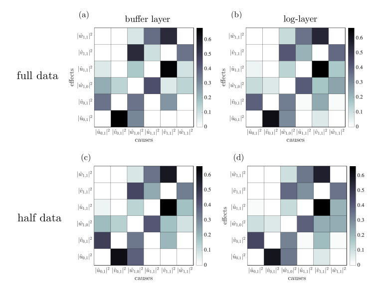
More quantitatively, the statistical significance of the values of $T_{j\rightarrow i}$ associated with $\tilde{T}_{j\rightarrow i}>0.3$ are evaluated under null hypothesis (H0) of no transfer entropy among variables. A new transfer entropy $T_{j\rightarrow i}^{\mathrm{H0}}$ is estimated replacing $\mathcal{V}_{j}$ by a surrogate signal $\mathcal{V}_{j}^{\mathrm{H0}}$ synthetically generated from the transitional probability distribution of the actual sample. The methodology utilised is block bootstrapping preserving the dependencies within each time series (Kreiss & Lahiri, 2012). The procedure is repeated thousand times for each $j=1,...,6$ to produce multiple $\mathcal{V}_{j}^{\mathrm{H0}}$, which yield a distribution of transfer entropies under the null hypothesis of no causality . The p-value associated with the null hypothesis is then computed by the probability of $T_{j\rightarrow i}^{\mathrm{H0}}$ being larger than the probability of the actual estimated value of $T_{j\rightarrow i}$. The details of the procedure are documented in Thomas & Julia (2013). The p-values, reported in figure 10, are below the level of significance $\alpha=0.05$ and the null hypothesis is rejected.

Figure 10: Statistical significance: p-values of $T_{j\rightarrow i}$ for (a) the buffer layer and (b) the log layer. The values covered by the colorbar ranges from $\alpha=0.00$ to $\alpha=0.02$.

References

- Agostini & Leschziner (2019) Agostini, L. & Leschziner, M. 2019 The connection between the spectrum of turbulent scales and the skin-friction statistics in channel flow at . J. Fluid Mech. 871, 22–51.
- Alizard (2015) Alizard, Frédéric 2015 Linear stability of optimal streaks in the log-layer of turbulent channel flows. Phys. Fluids 27 (10), 105103.
- Andersson et al. (2001) Andersson, Paul, Brandt, Luca, Bottara, Alessandro & Henningson, Dan S. 2001 On the breakdown of boundary layer streaks. J. Fluid Mech. 428, 29–60.
- Bae et al. (2018a) Bae, H. J., Encinar, M. P. & Lozano-Durán, A. 2018a Causal analysis of self-sustaining processes in the logarithmic layer of wall-bounded turbulence. J. Phys.: Conf. Series 1001, 012013.
- Bae et al. (2018b) Bae, H. J., Lozano-Durán, A., Bose, S. T. & Moin, P. 2018b Dynamic wall model for the slip boundary condition in large-eddy simulation. J. Fluid Mech. pp. 400–432.
- Bae et al. (2018c) Bae, H. J., Lozano-Durán, A., Bose, S. T. & Moin, P. 2018c Turbulence intensities in large-eddy simulation of wall-bounded flows. Phys. Rev. Fluids 3, 014610.
- Bailey et al. (2008) Bailey, S. C. C., Hultmark, M., Smits, A. J. & Schultz, M. P. 2008 Azimuthal structure of turbulence in high Reynolds number pipe flow. J. Fluid Mech. 615, 121–138.
- Barnett et al. (2009) Barnett, Lionel, Barrett, Adam B. & Seth, Anil K. 2009 Granger causality and transfer entropy are equivalent for Gaussian variables. Phys. Rev. Lett. 103, 238701.
- Beebee et al. (2012) Beebee, H., Hitchcock, C. & Menzies, P. 2012 The Oxford Handbook of Causation. OUP Oxford.
- Bullock et al. (1978) Bullock, K. J., Cooper, R. E. & Abernathy, F. H. 1978 Structural similarity in radial correlations and spectra of longitudinal velocity fluctuations in pipe flow. J. Fluid Mech. 88, 585–608.
- Butler & Farrell (1993) Butler, K. M. & Farrell, B. F. 1993 Optimal perturbations and streak spacing in wall-bounded turbulent shear flow. Phys. Fluids A 5, 774.
- Cardesa et al. (2017) Cardesa, J. I., Vela-Martín, A. & Jiménez, J. 2017 The turbulent cascade in five dimensions. Science 357 (6353), 782–784.
- Cassinelli et al. (2017) Cassinelli, Andrea, de Giovanetti, Matteo & Hwang, Yongyun 2017 Streak instability in near-wall turbulence revisited. J. Turb. 18 (5), 443–464.
- Cerbus & Goldburg (2013) Cerbus, R. T. & Goldburg, W. I. 2013 Information content of turbulence. Phys. Rev. E 88, 053012.
- Chandran et al. (2017) Chandran, Dileep, Baidya, Rio, Monty, Jason P. & Marusic, Ivan 2017 Two-dimensional energy spectra in high-Reynolds-number turbulent boundary layers. J. Fluid Mech. 826, R1.
- Cheng et al. (2019) Cheng, C., Li, W., Lozano-Durán, A. & Liu, H. 2019 Identity of attached eddies in turbulent channel flows with bidimensional empirical mode decomposition. J. Fluid Mech. 870, 1037–1071.
- Chernyshenko & Baig (2005) Chernyshenko, S. I. & Baig, M. F. 2005 The mechanism of streak formation in near-wall turbulence. J. Fluid Mech. 544, 99–131.
- Chorin (1968) Chorin, A. J. 1968 Numerical solution of the Navier-Stokes equations. Math. Comput. 22 (104), 745–762.
- Cossu & Hwang (2017) Cossu, C. & Hwang, Y. 2017 Self-sustaining processes at all scales in wall-bounded turbulent shear flows. Philos. Trans. Royal Soc. A 375 (2089).
- Darbellay & Vajda (1999) Darbellay, G. A. & Vajda, I. 1999 Estimation of the information by an adaptive partitioning of the observation space. IEEE Trans. Inf. Theory 45 (4), 1315–1321.
- Davidson et al. (2006) Davidson, P. A., Nickels, T. B. & Krogstad, P.-Å. 2006 The logarithmic structure function law in wall-layer turbulence. J. Fluid Mech. 550, 51–60.
- Del Álamo & Jiménez (2006) Del Álamo, J. C. & Jiménez, J. 2006 Linear energy amplification in turbulent channels. J. Fluid Mech. 559, 205–213.
- Del Alamo et al. (2004) Del Alamo, J. C., Jiménez, J., Zandonade, P. & Moser, R. D. 2004 Scaling of the energy spectra of turbulent channels. J. Fluid Mech. 500, 135–144.
- Del Álamo et al. (2006) Del Álamo, J. C., Jiménez, J., Zandonade, P. & Moser, R. D. 2006 Self-similar vortex clusters in the turbulent logarithmic region. J. Fluid Mech. 561, 329–358.
- Dong et al. (2017) Dong, S., Lozano-Durán, A., Sekimoto, A. & Jiménez, J. 2017 Coherent structures in statistically stationary homogeneous shear turbulence. J. Fluid Mech. 816, 167–208.
- Duan et al. (2013) Duan, P., Yang, F., Chen, T. & Shah, S. L. 2013 Direct causality detection via the transfer entropy approach. IEEE Trans. Control Syst. Technol. 21 (6), 2052–2066.
- Eddington (1929) Eddington, A. S. 1929 The nature of the physical world, 1st edn. Cambridge University Press Cambridge, England.
- Farrell et al. (2017) Farrell, B. F., Gayme, D. F. & Ioannou, P. J. 2017 A statistical state dynamics approach to wall turbulence. Philos. Trans. Royal Soc. A 375 (2089), 20160081.
- Farrell & Ioannou (2012) Farrell, Brian F. & Ioannou, Petros J. 2012 Dynamics of streamwise rolls and streaks in turbulent wall-bounded shear flow. J. Fluid Mech. 708, 149–196.
- Farrell et al. (2016) Farrell, B. F., Ioannou, P. J., Jiménez, J., Constantinou, N. C., Lozano-Durán, A. & Nikolaidis, M.-A. 2016 A statistical state dynamics-based study of the structure and mechanism of large-scale motions in plane poiseuille flow. J. Fluid Mech. 809, 290–315.
- Flores & Jiménez (2010) Flores, O. & Jiménez, J. 2010 Hierarchy of minimal flow units in the logarithmic layer. Phys. Fluids 22 (7), 071704.
- Fujita (1981) Fujita, T. T. 1981 Tornadoes and downbursts in the context of generalized planetary scales. J. Atm. Sci. 38 (8), 1511–1534.
- Gao & Er (2005) Gao, Y. & Er, M. J. 2005 Narmax time series model prediction: feedforward and recurrent fuzzy neural network approaches. Fuzzy Sets and Systems 150 (2), 331 – 350.
- Gencaga et al. (2015) Gencaga, De., Knuth, K. H. & Rossow, W. B. 2015 A recipe for the estimation of information flow in a dynamical system. Entropy 17 (1), 438–470.
- Granger (1969) Granger, C. W. J. 1969 Investigating causal relations by econometric models and cross-spectral methods. Econometrica pp. 424–438.
- Guala et al. (2006) Guala, M., Hommema, S. E. & Adrian, R. J. 2006 Large-scale and very-large-scale motions in turbulent pipe flow. J. Fluid Mech. 554, 521–542.
- Hahs & Pethel (2011) Hahs, D. W. & Pethel, S. D. 2011 Distinguishing anticipation from causality: Anticipatory bias in the estimation of information flow. Phys. Rev. Lett. 107, 128701.
- Haller (2015) Haller, G. 2015 Lagrangian coherent structures. Annu. Rev. Fluid Mech. 47 (1), 137–162.
- Hamilton et al. (1995) Hamilton, J. M., Kim, J. & Waleffe, F. 1995 Regeneration mechanisms of near-wall turbulence structures. J. Fluid Mech. 287, 317–348.
- Hellström et al. (2016) Hellström, L. H. O., Marusic, I. & Smits, A. J. 2016 Self-similarity of the large-scale motions in turbulent pipe flow. J. Fluid Mech. 792, R1.
- Hlavackova-Schindler et al. (2007) Hlavackova-Schindler, K., Palus, M., Vejmelka, M. & Bhattacharya, J. 2007 Causality detection based on information-theoretic approaches in time series analysis. Phys. Reports 441 (1), 1–46.
- Hof et al. (2010) Hof, B., de Lozar, A., Avila, M., Tu, X. & Schneider, T. M. 2010 Eliminating turbulence in spatially intermittent flows. Science 327 (5972), 1491–1494.
- Hoyas & Jiménez (2006) Hoyas, S. & Jiménez, J. 2006 Scaling of the velocity fluctuations in turbulent channels up to . Phys. Fluids 18 (1), 011702.
- Hoyas & Jiménez (2008) Hoyas, S. & Jiménez, J. 2008 Reynolds number effects on the Reynolds-stress budgets in turbulent channels. Phys. Fluids 20 (10), 101511.
- Hultmark et al. (2012) Hultmark, M., Vallikivi, M., Bailey, S.C.C. & Smits, A.J. 2012 Turbulent pipe flow at extreme Reynolds numbers. Phys. Rev. Lett. 108 (9), 094501.
- Hwang & Sung (2018) Hwang, J. & Sung, H.J. 2018 Wall-attached structures of velocity fluctuations in a turbulent boundary layer. J. Fluid Mech. 856, 958–983.
- Hwang & Sung (2019) Hwang, J. & Sung, H.J. 2019 Wall-attached clusters for the logarithmic velocity law in turbulent pipe flow. Phys. Fluids 31 (5), 055109.
- Hwang & Cossu (2010) Hwang, Y. & Cossu, C. 2010 Self-sustained process at large scales in turbulent channel flow. Phys. Rev. Lett. 105, 044505.
- Hwang & Cossu (2011) Hwang, Y. & Cossu, C. 2011 Self-sustained processes in the logarithmic layer of turbulent channel flows. Phys. Fluids 23 (6), 061702.
- Jiménez (2012) Jiménez, J. 2012 Cascades in wall-bounded turbulence. Annu. Rev. Fluid Mech. 44, 27–45.
- Jiménez (2013) Jiménez, J. 2013 How linear is wall-bounded turbulence? Phys. Fluids 25, 110814.
- Jiménez (2015) Jiménez, J. 2015 Direct detection of linearized bursts in turbulence. Phys. Fluids 27 (6), 065102.
- Jiménez (2018) Jiménez, J. 2018 Coherent structures in wall-bounded turbulence. J. Fluid Mech. 842, P1.
- Jiménez & Moin (1991) Jiménez, J. & Moin, P. 1991 The minimal flow unit in near-wall turbulence. J. Fluid Mech. 225, 213–240.
- Jiménez & Pinelli (1999) Jiménez, J. & Pinelli, A. 1999 The autonomous cycle of near-wall turbulence. J. Fluid Mech. 389, 335–359.
- Kaiser & Schreiber (2002) Kaiser, A. & Schreiber, T. 2002 Information transfer in continuous processes. Physica D 166 (1), 43 – 62.
- Kawahara et al. (2003) Kawahara, Genta, Jiménez, Javier, Uhlmann, Markus & Pinelli, Alfredo 2003 Linear instability of a corrugated vortex sheet – a model for streak instability. J. Fluid Mech. 483, 315–342.
- Kawahara et al. (2012) Kawahara, G., Uhlmann, M. & van Veen, L. 2012 The significance of simple invariant solutions in turbulent flows. Annu. Rev. Fluid Mech. 44 (1), 203–225.
- Kim & Lim (2000) Kim, J. & Lim, J. 2000 A linear process in wall-bounded turbulent shear flows. Phys. Fluids 12 (8), 1885–1888.
- Kim (1999) Kim, K. C. 1999 Very large-scale motion in the outer layer. Phys. Fluids 11 (2), 417–422.
- Klebanoff et al. (1962) Klebanoff, P. S., Tidstrom, K. D. & Sargent, L. M. 1962 The three-dimensional nature of boundary-layer instability. J. Fluid Mech. 12 (1), 1–34.
- Kline et al. (1967) Kline, S. J., Reynolds, W. C., Schraub, F. A. & Runstadler, P. W. 1967 The structure of turbulent boundary layers. J. Fluid Mech. 30 (04), 741–773.
- Kozachenko & Leonenko (1987) Kozachenko, L. F. & Leonenko, N. N. 1987 Sample estimate of the entropy of a random vector. Probl. Peredachi Inf. 23 (2), 9–16.
- Kraskov et al. (2004) Kraskov, A., Stögbauer, H. & Grassberger, P. 2004 Estimating mutual information. Phys. Rev. E 69, 066138.
- Kreiss & Lahiri (2012) Kreiss, J.-P. & Lahiri, S. N. 2012 Bootstrap methods for time series. In Time Series Analysis: Methods and Applications (ed. Tata Subba Rao, Suhasini Subba Rao & C.R. Rao), Handbook of Statistics, vol. 30, pp. 3 – 26. Elsevier.
- Kühnen et al. (2018) Kühnen, J., Song, B., Scarselli, D., Budanur, N. B., Riedl, M., Willis, A. P., Avila, M. & Hof, B. 2018 Destabilizing turbulence in pipe flow. Nat. Phys. 14 (4), 386–390.
- Landahl & Landahlt (1975) Landahl, M. T. & Landahlt, M. T. 1975 Wave breakdown and turbulence. SIAM J. Appl. Math 28, 735–756.
- Liang (2014) Liang, X. S. 2014 Unraveling the cause-effect relation between time series. Phys. Rev. E 90 5-1, 052150.
- Liang & Kleeman (2006) Liang, X. S. & Kleeman, R. 2006 Information transfer between dynamical system components. Phys. Rev. Lett. 95, 244101.
- Liang & Lozano-Durán (2017) Liang, X. S. & Lozano-Durán, A. 2017 A preliminary study of the causal structure in fully developed near-wall turbulence. CTR - Proc. Summer Prog. pp. 233–242.
- Lin et al. (1996) Lin, T., Horne, B. G., Tino, P. & Giles, C. L. 1996 Learning long-term dependencies in narx recurrent neural networks. IEEE Trans. Neural Netw. Learn. Syst 7 (6), 1329–1338.
- Lozano-Durán & Bae (2019) Lozano-Durán, A. & Bae, H. J. 2019 Characteristic scales of Townsend’s wall-attached eddies. J. Fluid Mech. 868, 698–725.
- Lozano-Durán et al. (2012) Lozano-Durán, A., Flores, O. & Jiménez, J. 2012 The three-dimensional structure of momentum transfer in turbulent channels. J. Fluid Mech. 694, 100–130.
- Lozano-Durán et al. (2018a) Lozano-Durán, A., Hack, M. J. P. & Moin, P. 2018a Modeling boundary-layer transition in direct and large-eddy simulations using parabolized stability equations. Phys. Rev. Fluids 3, 023901.
- Lozano-Durán & Jiménez (2014a) Lozano-Durán, A. & Jiménez, J. 2014a Effect of the computational domain on direct simulations of turbulent channels up to . Phys. Fluids 26 (1), 011702.
- Lozano-Durán & Jiménez (2014b) Lozano-Durán, A. & Jiménez, J. 2014b Time-resolved evolution of coherent structures in turbulent channels: characterization of eddies and cascades. J. Fluid. Mech. 759, 432–471.
- Lozano-Durán et al. (2018b) Lozano-Durán, A., Karp, M. & Constantinou, N. C. 2018b Wall turbulence with constrained energy extraction from the mean flow. Center for Turbulence Research - Annual Research Briefs pp. 209–220.
- Mansour et al. (1988) Mansour, N. N., Kim, J. & Moin, P. 1988 Reynolds-stress and dissipation-rate budgets in a turbulent channel flow. J. Fluid Mech. 194, 15–44.
- Marusic et al. (2010) Marusic, I., Mathis, R. & Hutchins, N. 2010 Predictive model for wall-bounded turbulent flow. Science 329 (5988), 193–196.
- Marusic & Monty (2019) Marusic, I. & Monty, J. P. 2019 Attached eddy model of wall turbulence. Annu. Rev. Fluid Mech. 51, 49–74.
- McCulloch & Pitts (1943) McCulloch, W. S. & Pitts, W. 1943 A logical calculus of the ideas immanent in nervous activity. Bull. Math. Biophys. 5 (4), 115–133.
- McKeon (2017) McKeon, B. J. 2017 The engine behind (wall) turbulence: perspectives on scale interactions. J. Fluid Mech. 817, P1.
- McKeon et al. (2004) McKeon, B. J., Li, J., Jiang, W., Morrison, J. F. & Smits, A. J. 2004 Further observations on the mean velocity distribution in fully developed pipe flow. J. Fluid Mech. 501, 135–147.
- Mizuno & Jiménez (2011) Mizuno, Y. & Jiménez, J. 2011 Mean velocity and length-scales in the overlap region of wall-bounded turbulent flows. Phys. Fluids 23 (8), 085112.
- Moarref et al. (2013) Moarref, R., Sharma, A. S., Tropp, J. A. & McKeon, B .J. 2013 Model-based scaling of the streamwise energy density in high-Reynolds-number turbulent channels. J. Fluid Mech. 734, 275–316.
- Monty et al. (2007) Monty, J. P., Stewart, J. A., Williams, R. C. & Chong, M. S. 2007 Large-scale features in turbulent pipe and channel flows. J. Fluid Mech. 589, 147–156.
- Morrison & Kronauer (1969) Morrison, W. R. B. & Kronauer, R. E. 1969 Structural similarity for fully developed turbulence in smooth tubes. J. Fluid Mech. 39 (1), 117–141.
- Onsager (1949) Onsager, L. 1949 Statistical hydrodynamics. Il Nuovo Cimento 6, 279–287.
- Orlandi (2000) Orlandi, P. 2000 Fluid Flow Phenomena: A Numerical Toolkit. Springer.
- Orr (1907) Orr, W. M’F. 1907 The stability or instability of the steady motions of a perfect liquid and of a viscous liquid. Part II: A viscous liquid. Math. Proc. Royal Ir. Acad. 27, 69–138.
- Paluš (1995) Paluš, M. 1995 Testing for nonlinearity using redundancies: quantitative and qualitative aspects. Physica D 80 (1), 186 – 205.
- Panton (2001) Panton, R. L. 2001 Overview of the self-sustaining mechanisms of wall turbulence. Prog. Aerosp. Sci. 37 (4), 341–383.
- Park et al. (2011) Park, J., Hwang, Y. & Cossu, C. 2011 On the stability of large-scale streaks in turbulent couette and poiseulle flows. Comptes Rendus Mécanique 339 (1), 1 – 5.
- Pearl (2009) Pearl, J. 2009 Causality: Models, Reasoning and Inference, 2nd edn. New York, NY, USA: Cambridge University Press.
- Perry & Abell (1975) Perry, A. E. & Abell, C. J. 1975 Scaling laws for pipe-flow turbulence. J. Fluid Mech. 67, 257–271.
- Perry & Abell (1977) Perry, A. E. & Abell, C. J. 1977 Asymptotic similarity of turbulence structures in smooth- and rough-walled pipes. J. Fluid Mech. 79, 785–799.
- Perry & Chong (1982) Perry, A. E. & Chong, M. S 1982 On the mechanism of wall turbulence. J. Fluid Mech. 119 (119), 173–217.
- Perry et al. (1986) Perry, A. E., Henbest, S. & Chong, M. S. 1986 A theoretical and experimental study of wall turbulence. J. Fluid Mech. 165, 163–199.
- Perry & Marusic (1995) Perry, A. E. & Marusic, I. 1995 A wall-wake model for the turbulence structure of boundary layers. Part 1. Extension of the attached eddy hypothesis. J. Fluid Mech. 298, 361–388.
- Prokopenko & Lizier (2014) Prokopenko, M. & Lizier, J. T. 2014 Transfer entropy and transient limits of computation. Sci. Rep. 4, 5394.
- Pujals et al. (2009) Pujals, Gregory, García-Villalba, Manuel, Cossu, Carlo & Depardon, Sebastien 2009 A note on optimal transient growth in turbulent channel flows. Phys. Fluids 21 (1), 015109.
- Richardson (1922) Richardson, L. F. 1922 Weather Prediction by Numerical Process. Cambridge University Press.
- Robinson (1991) Robinson, S. K. 1991 Coherent motions in the turbulent boundary layer. Annu. Rev. Fluid Mech. 23 (1), 601–639.
- Schoppa & Hussain (2002) Schoppa, W. & Hussain, F. 2002 Coherent structure generation in near-wall turbulence. J. Fluid Mech. 453, 57–108.
- Schreiber (2000) Schreiber, T. 2000 Measuring information transfer. Phys. Rev. Lett. 85, 461.
- Sekimoto et al. (2016) Sekimoto, A., Dong, S. & Jiménez, J. 2016 Direct numerical simulation of statistically stationary and homogeneous shear turbulence and its relation to other shear flows. Phys. Fluids 28 (3), 035101.
- Shannon (1948) Shannon, C. E. 1948 A mathematical theory of communication. Bell Syst. Tech. J 27 (3), 379–423.
- Sirovich & Karlsson (1997) Sirovich, L. & Karlsson, S. 1997 Turbulent drag reduction by passive mechanisms. Nature 388, 753.
- Smits et al. (2011) Smits, A. J., McKeon, B. J. & Marusic, I. 2011 High-Reynolds number wall turbulence. Annu. Rev. Fluid Mech. 43 (1), 353–375.
- Spinney et al. (2016) Spinney, R. E., Lizier, J. T. & Prokopenko, M. 2016 Transfer entropy in physical systems and the arrow of time. Phys. Rev. E 94, 022135.
- Stokes & Purdon (2017) Stokes, P. A. & Purdon, P. L. 2017 A study of problems encountered in granger causality analysis from a neuroscience perspective. Proc. Natl. Acad. Sci. U.S.A 114 (34), E7063–E7072.
- Swearingen & Blackwelder (1987) Swearingen, Jerry D. & Blackwelder, Ron F. 1987 The growth and breakdown of streamwise vortices in the presence of a wall. J. Fluid Mech. 182, 255–290.
- Thomas & Julia (2013) Thomas, D. & Julia, P. F. 2013 Using transfer entropy to measure information flows between financial markets. Studies in Nonlinear Dynamics & Econometrics 17 (1), 85–102.
- Tissot et al. (2014) Tissot, G., Lozano-Durán, A., Jiménez, J., Cordier, L. & Noack, B. R. 2014 Granger causality in wall-bounded turbulence. J. Phys. Conf. Ser 506 (1), 012006.
- Tomkins & Adrian (2003) Tomkins, C. D. & Adrian, R. J. 2003 Spanwise structure and scale growth in turbulent boundary layers. J. Fluid Mech. 490, 37–74.
- Townsend (1976) Townsend, A. A. 1976 The structure of turbulent shear flow. Cambridge University Press.
- Vallikivi et al. (2015) Vallikivi, M., Ganapathisubramani, B. & Smits, A. J. 2015 Spectral scaling in boundary layers and pipes at very high Reynolds numbers. J. Fluid Mech. 771, 303–326.
- Vaughan & Zaki (2011) Vaughan, N. J. & Zaki, T. A. 2011 Stability of zero-pressure-gradient boundary layer distorted by unsteady klebanoff streaks. J. Fluid Mech. 681, 116–153.
- Waleffe (1995) Waleffe, F. 1995 Hydrodynamic stability and turbulence: Beyond transients to a self-sustaining process. Stud. Appl. Math 95 (3), 319–343.
- Waleffe (1997) Waleffe, F. 1997 On a self-sustaining process in shear flows. Phys. Fluids 9 (4), 883–900.
- Wand & Jones (1994) Wand, M.P. & Jones, M.C. 1994 Kernel Smoothing. Taylor & Francis.
- Wray (1990) Wray, A. A. 1990 Minimal-storage time advancement schemes for spectral methods. Tech. Rep.. NASA Ames Research Center.
- Wu et al. (2017) Wu, X., Moin, P., Wallace, J. M., Skarda, J., Lozano-Durán, A. & Hickey, J.-P. 2017 Transitional–turbulent spots and turbulent–turbulent spots in boundary layers. Proc. Natl. Acad. Sci. 114 (27), E5292–E5299.