Optimal Investment to Enable Evolutionary Rescue

Abstract

“Evolutionary rescue” is the potential for evolution to enable population persistence in a changing environment. Even with eventual rescue, evolutionarily time lags can cause the population size to temporarily fall below a threshold susceptible to extinction. To reduce extinction risk given human-driven global change, conservation management can enhance populations through actions such as captive breeding. To quantify the optimal timing of, and indicators for engaging in, investment in temporary enhancement to enable evolutionary rescue, we construct a model of coupled demographic-genetic dynamics given a moving optimum. We assume “decelerating change”, as might be relevant to climate change, where the rate of environmental change initially exceeds a rate where evolutionary rescue is possible, but eventually slows. We analyze the optimal control path of an intervention to avoid the population size falling below a threshold susceptible to extinction, minimizing costs. We find that the optimal path of intervention initially increases as the population declines, then declines and ceases when the population growth rate becomes positive, which lags the stabilization in environmental change. In other words, the optimal strategy involves increasing investment even in the face of a declining population, and positive population growth could serve as a signal to end the intervention. In addition, a greater carrying capacity relative to the initial population size decreases the optimal intervention. Therefore, a one-time action to increase carrying capacity, such as habitat restoration, can reduce the amount and duration of longer-term investment in population enhancement, even if the population is initially lower than and declining away from the new carrying capacity.

1 Introduction

Global environmental change such as climate change has the potential to exceed the physiological tolerances of many organisms (Thomas et al. 2004; Urban 2015). For a population faced with environmental conditions outside its range of tolerance, persistence might occur through either a shift in its range or genetic adaption (Davis et al. 2005). Persistence via genetic adaptation in response to environmental change in a population that would otherwise perish is called “evolutionary rescue” (ER, Gomulkiewicz and Holt 1995; Carlson et al. 2014).

To date, theory on evolutionary rescue has focused on two situations where it can occur naturally. First, if the environmental optimum shifts suddenly, population size initially declines and eventually increases if enough genetic variation relative to the amount of change exists for adaptation to the new environment to occur (Gomulkiewicz and Holt 1995; Carlson et al. 2014). Such evolutionary rescue typically involves a period of low population size during which a population might be susceptible to factors such as demographic stochasticity, environmental stochasticity, Allee effects, inbreeding, and genetic drift (Lande 1998; Gilpin and Soule 1986). Second, if the environmental optimum is continuously changing at a constant rate, population growth declines, but populations with enough genetic variance relative to the rate of environmental change maintain population growth (Lynch and Lande 1993; Bürger and Lynch 1995). Therefore, populations with a given amount of genetic variation have a “critical rate” of environmental change above which ER cannot occur and growth rates become negative (Kopp and Matuszewski 2013).

As an example of a changing environmental optimum, climate change lies between sudden shift and gradual change. Depending on the amount of greenhouse gas emissions and therefore the rate of change in the climate (e.g., mean annual temperature), there might be a period of time where the rate of change in the optimum is “super-critical”, exceeding the rate where evolutionary rescue can occur. However, as the rate of change decelerates, as eventually occurs for all future climate scenarios (Meinshausen et al. 2011), evolution might play a greater role in population persistence.

Conservation management to increase the likelihood of evolutionary rescue and therefore population persistence under environmental change such as climate change can take two forms: mitigation and adaptation. Mitigation to reduce the rate or amount of change in temperature (e.g., by reducing greenhouse gas emissions) can increase the ability for evolution to keep up with the changing environment. However, for climate change, mitigation requires international cooperation (King 2004). Conservation management, however, most often occurs at local, regional, or national scales. Further, local efforts to mitigate emissions do not reduce locally-felt effects of climate change. Without a direct role in mitigating climate change, then, conservation management must focus on “adaptation” in the anthropogenic sense, which in a conservation context involves promoting processes that increase the likelihood of population persistence (Stein et al. 2013). For the case of increasing the likelihood of ER, adaptation can involve reducing local stressors (e.g., Baskett et al. 2010) or enhancing population size to reduce the likelihood of a population falling below a threshold size at risk of extinction (Fraser 2008).

For decelerated change such as climate change, management interventions during the initial period when change might be super-critical could preserve the option for longer-term ER to occur. Interventions inevitably differ in whether they have a temporary or permanent effect on population size and growth rate. Interventions with potentially permanent effects include habitat restoration (Bradshaw 1996) and removal of invasive predators or competitors (Myers et al. 2000). Interventions with temporary effects, i.e., which only affect the population transiently, include resource provisioning (Ruffino et al. 2014), head-starting (captive rearing of a vulnerable early life stage), and captive breeding (Heppell et al. 1996; Griffiths and Pavajeau 2008). Climate change threatens a variety of species that are also targets for captive breeding. For example, climate change-driven changes to river flow and temperature can negatively affect Pacific salmon (Crozier et al 2008), and hatcheries (i.e., hatching of eggs in captivity to release into the wild at early life stages) are a long-standing tool to increase salmon population sizes (Naish et al 2008). Analogously, increases in extreme temperature events threaten the persistence of tropical corals (Bellwood et al 2004), and ”coral gardening” (i.e., nursery-based growth of small fragments into larger corals to outplant into the wild) can provide large-scale population supplementation for corals (Lirman and Schopmeyer 2016). Yet, captive rearing and breeding have the potential to involve unintended negative consequences for wild populations such as domestication, the negative effects of which can accumulate over multiple generations, which leads to recommendations to limit the use and duration of such programs (Snyder et al. 1996; Fraser 2008). In addition, the ultimate success of captive breeding and rearing in leading to population persistence without requiring indefinite intervention (i.e., conservation reliance sensu Scott et al. 2010), depends on addressing the factors that originally lead to population declines (Fraser 2008).

In addition to the potential to incur unintended consequences, interventions such as captive breeding and rearing can be costly (Snyder et al. 1996) and budgets are inevitably limited. Thus, a key management question is the efficient allocation of resources both over time and among populations. For example, when is it bioeconomically optimal to invest in an intervention and for how long should a manager keep investing? Furthermore, what biological or economic indicators can be used to make such decisions? Investing early may help build population abundance and reduce the effects of environmental change. Alternatively, for populations initially close to carrying capacity and thus self-regulating, early investments may have less effect per dollar spent. Self-regulation might also determine the efficacy of pairing an investment with a temporary effect such as captive rearing with an action with a permanent effect such as habitat restoration. In particular, a one-time investment to permanently increase carrying capacity might reduce the investment necessary in captive rearing by decreasing the role of self-regulation, or it might have little effect if self-regulation has little effect on population dynamics when populations are initially declining under rapid environmental change. Economic factors that might further influence the pattern of investment include budget constraints and the rate of discounting. Possible indicators for optimal timing of investment include a population growth rate, population size, or the rate of environmental change.

Here we quantify the bioeconomically optimal investment schedule for an evolving population undergoing decelerating environmental change. The objective of the regulator is to minimize costs (and therefore the amount of intervention) given a goal of avoiding extinction. To this end, we develop a model that couples the demographic dynamics necessary to account for extinction risk, the genetic dynamics necessary to account for ER, and the economic dynamics necessary to determine the optimal investment schedule. Our biological model assumes a moving optimum where the rate initially exceeds the critical rate for ER to occur and eventually slows to that rate (Figure 1a). Without intervention the population size will decline below a critical threshold considered at risk of extinction (Figure 1b). We also assume a management intervention that temporarily increases population growth (e.g. resource provisioning, head-starting, or captive breeding) but is costly. We analyze the pattern of intervention that minimizes costs, subject to the constraint of keeping the population above a critical size, given different values for the carrying capacity, discount rate, and annual budget.

Figure 1: Under “decelerating environmental change” (a), the optimum trait value (solid line) initially increases rapidly, then slows to the critical rate where evolutionary rescue can occur at time $t_{\text{safe}}$ (vertical dash-dot line). The population mean trait (dashed line) initially lags from the optimum but after $t_{\text{safe}}$ closes the gap. Without intervention to supplement or improve population growth (b), the population will fall below critically low size susceptible to extinction (gray line) for an extended period, but it does eventually increase. Meanwhile, the genetic variance decreases with decreasing population size (c) according to the stochastic house-of-cards approximation.

2 Materials and Methods

Our bioeconomic model consists of a sub-model for the environment, the biological response of the population, and the economic costs of control (i.e., management interventions to improve population growth). Combining these sub-models, we pose an control problem for optimally-scheduling spending on the control while avoiding extinction. We analyze the problem numerically to find the optimal solution.

2.1 Model

2.1.1 Changing environment

To represent environmental change, we consider an environmental optimum $\theta(t)$ that changes in time with rate $k(t)$. Initially, the rate of change $k_{0}$ exceeds a critical rate $k_{c}$, above which evolution cannot prevent population declines (e.g., as in Lynch and Lande 1993) but it slows to less than $k_{c}$ by time $t_{\text{safe}}$. We assume the optimum changes deterministically,

$$\theta(t)=k(t)t$$ (1)

where

$$k(t)=\begin{cases}k_{c}\left(\kappa_{0}-\frac{\kappa_{0}-\kappa_{\text{min}}}{t_{\text{safe}}-t_{0}}t\right)\quad\text{for}\>t<t_{\text{safe}}\\ \kappa_{\text{min}}k_{c}\quad\text{for}\>t\geq t_{\text{safe}}\end{cases},$$ (2)

and with $\kappa_{0}>1$ and $\kappa_{\text{min}}<1$.

2.1.2 Biological dynamics

Our model follows the joint demographic-genetic dynamics of population size $N(t)$ and genetic distribution $\psi_{t}(a)$ of quantitative trait $a$ under stabilizing selection toward the optimum $\theta(t)$. We assume the order of events in the life-cycle is mating, density-dependence, then viability selection. Note our life-cycle ordering corresponds to hard selection (Wallace 1975). We also assume random mating, a closed population, and discrete generations. Finally, we assume many genes of small effect additively contribute to the genotype such that, by the central limit theorem, the genetic distribution $\psi(a)$ is normal (Lande 1976). Therefore, we define the genetic distribution by its evolving mean $\bar{a}_{t}$ and genetic variance $\sigma^{2}_{a}(N)$, which depends on the census population size to accuont for the effects of drift, $\psi_{t}(a)=\exp(-(a-\bar{a}_{t})^{2}/(2\sigma^{2}_{a}(N)))/\sqrt{2\pi\sigma^{2}_{a}(N)}$. Specifically we use the stochastic house of cards approximation of mutation-selection-drift balance for the genetic variance $\sigma_{a}$, as in Bürger and Lynch (1995), which we specify below.

In the mating step, the number of offspring per individual is $R_{0}$, and the assumption of random mating means that the genetic distribution is unchanged (Lande and Arnold 1983). In the density dependence step, we apply a saturating Beverton-Holt (1957) function with parameter $K$ determining carrying capacity (equal to $(R_{0}-1)K$), where density-dependent survival is independent of genotype. Therefore, encapsulating both reproduction and density dependence, the pre-selection growth function $g(N(t))=\frac{R_{0}N(t)}{1+N(t)/K}$ depends solely on the population size $N(t)$.

In the viability selection step, we convert genotype $a$ to phenotype $z$ given random environmental contribution to the phenotype $e$ normally distributed with mean 0 and variance $\sigma_{e}^{2}$, i.e. we account for imperfect inheritance but not phenotypic plasticity, such that $z=a+e$. Therefore, the phenotype probability distribution given a particular genotype is $P(z|a)=\exp(-(z-a)^{2}/(2\sigma_{e}^{2}))/\sqrt{2\pi\sigma_{e}^{2}}$. We then apply stabilizing selection for $\theta(t)$ given width of the fitness function (inverse of selection strength) $\omega^{2}$, such that fitness $W(z)=\exp(-(z-\theta(t))^{2}/\omega^{2}$. Applying selection to the genetic distribution yields the genotypic distribution at time $t$ as $\psi^{\prime}_{t}(a)=\int W(z)P(z|a)\psi_{t}(a)dz$, where the overall population fitness in generation $t$, equivalent to the proportion of the population that survives viability selection, is

$$\bar{W}(t)=\int\psi^{\prime}_{t}(a)da=\sqrt{\frac{\omega^{2}}{\omega^{2}+\sigma_{a}^{2}(N)+\sigma_{e}^{2}}}e^{-\frac{(\bar{a}_{t}-\theta(t))^{2}}{2(\omega^{2}+\sigma_{a}^{2}(N)+\sigma_{e}^{2})}}.$$ (3)

Therefore, as $\theta(t)$ changes each generation, mean fitness changes as well, cascading into changes in the population size and genetic distribution. For the population size, applying fitness-dependent survival after growth yields the recursion of $N(t+1)=\bar{W}(t)g(N(t))$. Using the above-described growth function that accounts for reproduction and density dependence, the overall natural population growth factor (excluding any intervention-based growth), calculated from $N(t+1)/N(t)$, is:

$$\bar{\lambda}(t,N)=\frac{\bar{W}(t)R_{0}}{1+N(t)/K}.$$ (4)

For the genetic dynamics, we normalize the genetic distribution $\psi_{t+1}(a)=\psi^{\prime}_{t}(a)/\bar{W}(t)$ to yield the new genotypic distribution with mean

$$\bar{a}_{t+1}=\frac{\theta(t)\sigma_{a}^{2}(N)+(\omega^{2}+\sigma_{e}^{2})\bar{a}_{t}}{\omega^{2}+\sigma_{a}^{2}(N)+\sigma_{e}^{2}}.$$ (5)

To simplify notation, we let $s(N)=\sigma_{a}^{2}(N)/(\omega^{2}+\sigma_{a}^{2}(N)+\sigma_{e}^{2})$ and rearrange to arrive at the mean genotype recursion

$$\bar{a}_{t+1}=\bar{a}_{t}+s(\theta(t)-\bar{a}(t)).$$ (6)

In these recursions we use the stochastic house of cards (SHC) approximation as in Bürger and Lynch (1995): first, setting the effective population size to $N_{e}(N)=\frac{2R_{0}}{2R_{0}-1}N$ and, second, using the formula $\sigma_{a}^{2}(N)=\frac{2V_{m}N_{e}(N)}{1+\alpha^{2}N_{e}(N)/(\omega^{2}+\sigma_{e}^{2})}$, where $\alpha^{2}$ is the genetic effect size variance of a new mutation and $V_{m}$ is the mutational variance. The SHC approximation accounts for the equilibirium effect of changing population size on genetic variance with a fixed optimum, constant mutational variance, effect size, and demography; using it for dynamic population size change as we do (consistent with Bürger and Lynch 1995) is inexact but caputres the coarse-scale effect of population size change on genetic variance (Kopp and Matuszewski 2013).

Our model for a decelerating optimum, eq. (1), requires choosing a value for the parameter defining a critical rate of change $k_{c}$ beyond which ER cannot occur. To do so, we use an approximate model with constant environmental change $\theta(t)=\tilde{k}t$ given $\tilde{k}$ constant in time. Then the model is identical to a simplified version of Bürger and Lynch (1995) presented in Kopp and Matuszewski (2013), and the population reaches a dynamic equilibrium where the trait lags the optimum by the value $\tilde{k}(\sigma_{a}^{2}(N)+\omega^{2}+\sigma_{e}^{2})/\sigma_{a}^{2}(N)$. Using this, Kopp and Matuszewski (2013) calculate the value of $\tilde{k}$ at self-replacement such that for any $\tilde{k}>k_{c}$ the population is below replacement (i.e. $\bar{\lambda}<1$) and the population will decline, as

$$k_{c}(N)=\sigma_{a}^{2}(N)\sqrt{\frac{2\log{\left(R_{0}\sqrt{s(N)}\right)}}{\sigma_{a}^{2}(N)+\omega^{2}+\sigma_{e}^{2}}}.$$ (7)

Here, we still employ the SHC approximation, such that the population size affects the critical rate $k_{c}(N)$, which thus should be computed for the minimum population size reached during ER. For this, we use a population size, $N=N_{c,g}$ below which negative factors beyond demographic stochasticity (e.g., mutational meltdown) may cause rapid population extinction.

2.1.3 The control: improving population growth in situ

We consider a control that temporarily modifies the population growth rate in situ, resulting in changes in population dynamics and costs to the manager. If the control increases the population by a factor $v(t)\geq 1$ at each time $t$ simultaneous with natural production $R_{0}$ then we replace the population size $N(t)$ with $N(t)v(t)$ in eq. (4), and the population dynamics with the intervention are

$$N(t+1)=N(t)v(t)\bar{\lambda}(t,v(t)N(t)).$$ (8)

The mean trait dynamics (eq. (6)) are unchanged.

We assume that interventions incur costs $c(v(t))$ that scale quadratically with the proportional increase in the growth rate. We also consider a yearly budget constraint.

2.2 Statement and analysis of the control problem

The control problem is to minimize costs $c(v(t))$ while avoiding population sizes below a critically low level, $N_{c,s}$, assuming the growth rate eq. (4) determines the biological dynamics, values of the control within the feasible set $v(t)\in\Omega$, and with discount rate $\Delta$ across the time horizon $T$,

$${\rm min}_{\Omega}\;\sum_{t}c(v(t))\left(\frac{1}{1+\Delta}\right)^{t}\quad\forall t\leq T$$ (9a)

$$\textrm{subject to }N(t)\geq N_{c,s},\;v(t)\geq 1,$$ (9b)

where the dynamics of population $N(t)$ are defined in eq. (8).

To analyze the discrete-time optimal control problem eq. (9a) we specify concrete functional forms for the costs and add constraints based on the population dynamics. For a control $v(t)$ we assume a simple cost function $c(v(t))=\log v(t)^{2}$, which results in a cost of 0 when $v(t)=1$ and quadratic costs for log-scale intervention $u(t)=\log v(t)$. The objective at each time (neglecting discounting) is then $u(t)^{2}$. We also let $x(t)=\log N(t)$, and denote the log-scale initial population size as $x_{init}=\log N(0)$, which enters the problem as an equality constraint at time 0. We denote the log-scale critical population size as $x_{c}=\log N_{c,s}$, which enters the problem as an inequality constraint at each time. In log scale, the recursion for population growth from eq. (8) is $x(t+1)=u(t)+x(t)+\log\bar{\lambda}(t,\exp(x(t)+u(t)))$, these dynamics enter the problem as an equality constraint at each time. Finally, we assume a budget constraint with a constant budget $b$ within each year, which imposes another inequality constraint at each time. Accounting for all of this, the constrained control problem is

$$\min_{u(t)}\sum^{T-1}_{t=0}u(t)^{2}\left(\frac{1}{1+\Delta}\right)^{t}$$ subject to (10a)

$$x(t+1)-x(t) =u(t)+\log\bar{\lambda}\left(t,\exp(u(t)+x(t))\right)\quad t=0,1,\dots T$$ (10b)

$$x(0) =x_{init}$$ (10c)

$$0 \leq u(t)\quad t=0,1,\dots T-1$$ (10d)

$$u(t)^{2} \leq b\quad t=0,1,\dots T-1$$ (10e)

$$x(t) \geq x_{c}\quad t=0,1,\dots T.$$ (10f)

2.2.1 Parameter choices and assumptions

To model a situation where the population is initially declining but could eventually recover (albeit having experience populations too low to persist), we assume $t_{\text{safe}}$, the time at which the rate of environmental change $k(t)$ in eq. (2) transitions from being greater than to being equal to the rate at which ER is possible, $k_{c}(N_{c,g})$, occurs within the time horizon, i.e., $t_{\text{safe}}\leq T$.

We chose the biological parameters to start in a space where, without intervention, the population initially declines to a low population size susceptible to stochasticity but not to deterministic extinction, as that is the parameter space where our central questions on the effects of intervention on ER are relevant. We also assume that the population initially is experiencing a sustainable rate of environmental change. See Table 1 for all default parameter values used. In addition to analyzing the optimal path of investment in intervention for these default values, we compare the optimal path under varying density-dependence $K=10,000$, $K=15,000$, or $K=20,000$ to explore the effect of population regulation, and a discount rate of $\Delta=$ 0 or 0.025 and a budget of $b=$ 0.01 or 0.02 to explore the effects of economic factors. In all cases, the initial genetic mean is the initial optimal phenotype $a_{0}=\theta(0)=0$ and the initial population size is set equal to the equilibrium population size with $K=10,000$ accounting for variance load $N(0)=\bar{W}(0)(R_{0}-1)K$ under the assumption that the environment is already changing at a rate $\kappa_{\text{min}}$ (this results in $N(0)\approx 3600$).

Table 1: Parameters and default values.

Parameter	Default Value	Description
$R_{0}$	1.5	Number of offspring per individual
$K$	15,000	Carrying capacity
$\omega^{2}$	50	Selectional variance (inverse of selection strength)
$\alpha^{2}$	0.05	Genetic effect size variance of a new mutation
$V_{m}$	0.001	Mutational variance
$\sigma_{e}^{2}$	0.5	Environmental contribution to phenotypic variance
$t_{\text{safe}}$	20	Time at which the rate of environmental change slows to a value where ER can occur
$\kappa_{0}$	2.5	Maximum rate of change (multiplied by $k_{c}(N_{c,g})$)
$\kappa_{\text{min}}$	0.95	Minimum range of change (multiplied by $k_{c}(N_{c,g})$)
$N_{c,g}$	500	Population size used for calculating critical rate of change $k_{c}$
$N_{c,s}$	1,000	Critical population size for extinction risk due to stochastic factors
$\Delta$	0.025	Discount rate
$b$	0.01	Annual budget

2.2.2 Model analysis

We numerically analyzed the system (10) with augmented Lagrangian minimization (Birgin and Martínez 2008) as implemented in the NLOPT library (Johnson 2016). This requires restating the problem as a constrained discrete-time optimal control problem (see, e.g., Chow 1997), with eq. (10)a as the objective to minimize, eqs. (10)b and (10)c as equality constraints and eqs. (10)d, (10)e, and (10)f as inequality constraints. See the supplementary methods (Online Resource 1) for code. For all parameter combinations, we set the initial control and population to a path found using a zero discount rate and a large number of iterations. For global optimization algorithms such as the one we employ, convergence is difficult to assess in general. For a convergence criterion, we considered a path optimal if the solver consistently converged upon it with an increasing number of iterations; see Appendix A.

3 Results

Given our choice of parameter space and assumption that the rate of environmental change starts greater than, and eventually shows to, a value where ER is possible (Figure 1a), without intervention population growth is initially negative and population size falls below a critically population vulnerable to extinction (Figure 1b). Eventually, as environmental change slows, population population growth will become positive (Figure 1b), with a U-shaped demographic trajectory analogous to ER models with sudden environmental shifts (Gomulkiewicz and Holt 1995; Carlson et al. 2014).

3.1 Optimal investment trajectory and indicators

The optimal trajectory for investment in intervention initially increases quickly, with investment peaking at or before the time when the population size reaches the minimum acceptable population size (Figure 2). Notably, investment increases even as the population is declining under the management intervention (Figure 2c). Thus, in this case, declining population under a management intervention does not imply that the strategy is non-optimal.

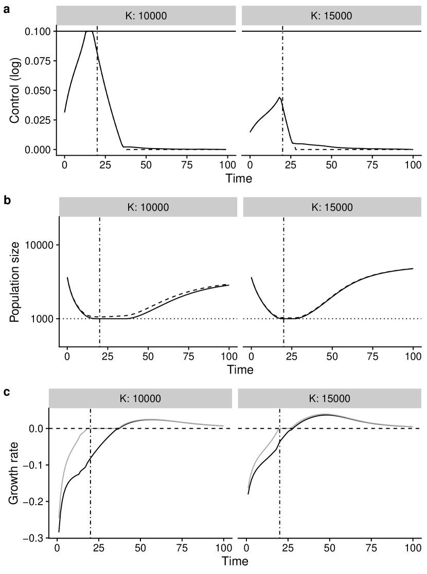
Figure 2: Details of the (a) optimal investment path, (b) population size, and (c) population growth rate ($\log\bar{\lambda}$) under the default parameter values (Table 1) with varying $K$. The strategy that minimizes costs to intervention while avoiding a population size below a threshold vulnerable to extinction (horizontal dotted line in B) results in an initial increase in investment, which peaks then decreases (a) in the same year that the growth rate including the intervention (gray line) transitions from negative to zero (stable; C); note that without the intervention population growth rate would still be negative (black line in C). Investment ramps down after the time $t_{\text{safe}}$ (vertical dash-dot line) when the rate of environmental change equals the critical rate where evolutionary rescue can occur, i.e. population growth can become positive without intervention (Figure 1).

Optimal investment then begins to slow in the year that the population growth rate, including effects of intervention (gray line in Figure 2c), transitions from population decline to stable. Investment reaches a very low level once population growth rate would be positive without the effects of intervention (Figure 2c); this occurs with some delay after the rate of change decreases to the critical rate $k_{c}$. Once that occurs, at time $t_{\text{safe}}$, the rate of environmental change is still positive, but at a rate slow enough for evolutionary rescue to occur if it were constant; however, intervention is still needed after $t_{\text{safe}}$ to reduce lag between the population mean trait and the optimal trait to a sustainable magnitude.

3.2 Factors that influence the optimal trajectory of investment

A carrying capacity further from the initial population size favors lower investment overall and shifts investment later in time (Figure 3). Compared to carrying capacity, the economic factors of discounting and budget constraints had weaker effects on the amount of investment in intervention (Figure 3-4). Greater discounting favors investing later in time (Figure 4) and weakens the need to ramp investment down to zero after positive population growth is achieved (with zero discounting investment goes to practically zero at this point; see Appendix, Figure 4).

Figure 3: Optimal control with varying carrying capacity (varying greyscale) and discount rate (varying linetype) for two yearly budgets. (a) Population sizes under the optimal path of investment in intervention, which includes the constraint of not allowing the population to fall below a size considered vulnerable to extinction (horizontal dotted line). (b) Optimal investment trajectory relative to the budget constraint (horizontal line), where investment ends when population growth is positive, lagged after the rate of change decreasing to the critical rate where evolutionary rescue can occur at $t_{\text{safe}}$ (vertical dash-dot line). Discount rates have little effect relative to that of carrying capacity. A carrying capacity closer to the initial population size (which corresponds to $K=10,000$) leads to initially-steeper population declines and earlier peak investment. The larger budget ($b=0.02$ per year) never constrains the solution. All solutions assume decelerating environmental change as in Figure 1a where the rate of environmental change decreases to the critical rate where evolutionary rescue can occur at $t_{\text{safe}}$ (vertical dash-dot line).

4 Discussion

We find that, with decelerating change, short-term investment in enhancing population growth can reduce extinction risk to allow for a combination of evolution and global-scale mitigation (resulting in deceleration of the optimum) to lead to long-term persistence. This occurs because at the time investment is stopped, the rate of change is within the population’s tolerance limits (see, e.g., Bürger and Lynch 1995). Optimal investment trajectories to conserving populations in the face of global stressors may initially mean doubling down on what appears to be a failing strategy due to ongoing population decline (Figure 2a,b). Mumby et al. (2017) provide a similar example where a declining system state is not a signal of improper management. In their analysis of coral reef management under climate change, they point out if managers and the public consider the unmanaged (or non-optimally managed) counterfactual scenario then this can alter perceptions of management utility. Such analyses are necessary to evaluate the effectivness of management and distinguish between those strategies that are actually failing and those which are optimial but still result in declines; our results demonstrate that such exercises may be needed to avoid a crisis of motivation when managing populations that are capable of evolutionary rescue.

In contrast to the trend or status of population size, under optimal management the trend in population growth rate (including management’s effect on population growth) reliably increases, at first becoming less negative and eventually leveling out to stable then increasing to persistence (positive population growth; Figure 2c). This indicates that trend in growth rate may provide a reliable signal of management efficacy as compared to the trend in population size. These same observations imply that timing of assessment matters: assessing the effect of an intervention prematurely may lead managers to dismiss what would be a successful strategy in the long run.

Overall, the optimal investment trajectory of initially increasing, then, as population growth stabilizes, decreasing, to stop when population growth is positive, is surprisingly robust to a wide array of economic assumptions and parameters, both qualitatively and quantitatively (Figure 3). Note that this unimodal investment trajectory is analogous to that in Lampert and Hastings (2014), focused on the optimal investment schedule for restoration to accelerate the recovery of a degraded system in a stable environment (without evolution). Much like the cessation of investment when evolutionary rescue can occur naturally in our model, the optimal investment trajectory in Lampert and Hastings (2014) ceases after at an “economic restoration threshold”, before full recovery has occurred. Both Lampert and Hastings (2014) and our study are examples of a phenomenon that is likely more general in conservation decisionmaking: optimal managment involves investing to a point when natural processes can complete recovery.

Carrying capacities closer to the initial population size led to earlier and greater investment in population enhancement (Figure 3), which indicates a significant role of density-dependent suppression of population growth even for declining populations. This result reflects the fact that per-capita reproduction decreases as the population approaches the carrying capacity, and again points to population growth serving as a more useful indicator than population size: while a population size near carrying capacity might, based on intuition, be considered to be not yet in need of support, the faster initial decline (due to stronger density dependence in combination with rapid environmental change) means that it actually requires greater initial intervention. In addition, this result indicates that a separate investment to permanently enhance carrying capacity, such as through restoration, can significantly reduce the investment necessary in short-term population enhancement, such as through captive rearing or breeding. A key next step in this analysis would be to analyze the optimal investment across actions with long-term and short-term effects; note that, unless the action with long-term effects enhances population growth rather than carrying capacity, investment in short-term population enhancement will always be necessary under our model assumptions given rapid environmental change leading to initial population declines.

4.1 Applications

Our model provides a generic representation of cases of systems where climate change might threaten near-term persistence and interventions to increase population size during such a period are feasible. Examples include climate change-driven changes to rivers treatening Pacific salmon Pacific salmon (Crozier et al 2008) whose populations can be supplemented via hatcheries (Naish et al 2008), and climate threats to the persistence of tropical corals (Bellwood et al 2004) whose populations can be supplemented via ”coral gardening” (Lirman and Schopmeyer 2016).

Direct application of our model to one of these cases would require empirical knowledge of both genetic potential and the change in the environmental optimum, as well as other biological parameters. Although such estimates of genetic parameters are often available (see, e.g., Carlson et al 2014) estimates of environmental optima are rare, but critical for predicting evolutionary responses to environmental change (Chevin et al 2010; Chevin et al 2017). Our analysis demonstrates how such predictions might be used by managers; the next step is to develop parameter estimates and models for specific settings. Such case-specific models would need to address not only biological parameters but policy choices, for example the quasi-extinction threshold, $N_{c,s}$. In fact, even the use of a threshold is a choice. For some cases, an alternative model where a explicit value is placed on existence of the population my be preferable.

4.2 Assumptions and analytical choices

As with any model, our model makes a number of simplifying assumptions for tractability. For example, we use a generic form of population enhancement that temporarily increases growth rate, which we associate with actions such as resource supplementation, head-starting, or captive breeding. As noted in the Introduction, such actions might incur unintended consequences such as domestication and reduced fitness, which we ignore with our assumption that the genetic dynamics (dynamics of $\bar{a}_{t}$) are independent of the intervention. For example, reductions in wild fitness occurs rapidly in Pacific salmon reared in hatcheries (Araki et al. 2008; reductions can occur within one generation, Christie et al. 2012). Incorporating such unintended fitness consequences of captive rearing would likely delay the evolutionary response in our model and therefore might increase the duration of intervention necessary given our constraint of maintaining a population size above a critical threshold, depending on how much an increase in program duration intensifies domestication selection. Quantitative genetic models indicate that one potential approach to reducing such unintended fitness consequences is to consistently target a combination of captive-reared and wild-reared individuals in the captive environment (Ford 2002; as opposed to captive-reared only, Baskett and Waples 2013). Alternatively, careful management of breeding’s effects on genetic variance in trait and fitness might prove an accelerator for evolution and be purposely used (as in “adaptive provenancing” sensu Weeks et al. 2011; or “assisted evolution” sensu Oppen et al. 2015), where the balance between domestication and assisted evolution effects would determine the efficacy of this approach.

One major omission from our modeled scenario is phenotypic plasticity. When phenotypes plastically respond to environmental change, this can facilitate adaptation to a changing environment (Chevin et al. 2010) and thus evolutionary rescue; the relationship between the environmental cue that affects phenotype and the environment of selection, however, is critical for determining whether plasticity increases the chances of evolutionary rescue (Ashander et al. 2016). However accounting for plasticity may be important in understanding the effects of climate change, as much of the response in traits observed to date owes to plasticity (Merilä and Hendry 2014). This may be especially true for species with complex life cycles involving many transitions between environments (e.g., Pacific salmon, Crozier et al. 2008).

Our modeled intervention to increase short-term population growth assumes immediate effect. In reality, many interventions, such as habitat restoration or removal of stressors like invasive species, might have delayed effects and require intervention over multiple years for a permanent effect to occur (Myers et al. 2000; Borja et al. 2010). In a discrete-time formulation such as ours, delays like this would likely result in greater investment earlier in time. These and other subtleties warrant investigation in future work on the interaction between microevolution and restoration, a topic of increasing import given climate change (Rice and Emery 2003).

In our analysis, we rely on a threshold population size $N_{c,s}$ to indicate extinction risk to factors such as demographic stochasticity, environmental stochasticity, Allee effects, inbreeding, and genetic drift. Although this approach is common, and may seem conservative (Gomulkiewicz and Holt 1995), it may mislead. Explicit analyses of demographic and genetic stochasticity can more effectively describe how extinction risk varies with factors such as genetic variance and indicate that minimum population size might better predict extinction risk than time below a threshold (Boulding and Hay 2001). However, for applications it is more common to set management goals in terms of population size as compared to actual extinction risk (Flather et al. 2011). In part, this may be because population size is easier to quantify than risk.

For our population dynamics, we further assume a saturating, Beverton-Holt (1957) form of density-dependent regulation, which ignores the potential for overcompensation (i.e., a decline, rather than saturation, at large population sizes, as in Ricker density dependence). Strong overcompensation would likely delay the optimal initial investment until after some population decline has occurred, such that enhanced population growth would not increase the population size beyond the overcompensatory level where large-scale declines would then occur. Analogously, an initial action to permanently increase carrying capacity and therefore weaken density dependence might have even a stronger effect under overcompensatory density dependence. However, we examined only a single life-cycle ordering (reproduction, density-dependence, viability selection), which corresponds to hard selection (Wallace 1975). Viability selection occurring before, rather than after, density dependence would likely reduce the role of increasing carrying capacity in decreasing the amount of investment necessary. Further, we examined only non-overlapping generations without age structure. The response of such populations is an intersting topic for future work, as it is unclear whether they would respond more or less rapidly than the case of non-overlapping generations studied here. On the one hand, overlapping generations with age structure can increase the maintenance of genetic variation (Ellner and Hairston 1994), and greater genetic variation can mean greater adaptive capacity and therefore more rapid evolutionary response. On the other hand, generation time is longer in such populations, resulting in slower evolutionary response.

We relied on standard assumptions for quantitative genetic models, which include a large number of loci contributing additively to a trait with a normal distribution (Lande 1976; Lande 1982). Such assumptions typically have minor effects on the predicted evolutionary trajectory (Turelli and Barton 1994). We did account for the effect of population size on genetic variance, where we used the stochastic house-of-cards (SHC) approximation as in Bürger and Lynch (1995). This captures the effect of how small population sizes will lower genetic variance, thus reducing the capacity for evolutionary rescue (Lynch and Lande 1993; Bürger and Lynch 1995; Gomulkiewicz and Holt 1995; Carlson et al. 2014) and therefore likely increase the amount and duration of investment necessary. Although, as Kopp and Matuszewski (2013) point out, the SHC approximation does not account for the effect of directional selection on increasing genetic variance, both this effect and the mutation-selection-drift balance modeled by the SHC occur only after some transient period; the SHC approximation likely captures the correct overall average effect of declining population size: reducing genetic variance.

Our major economic assumption is that cost of the intervention is quadratic in the amount of intervention. In reality, there might be decreasing costs, i.e., returns to scale, for supplementation programs. However, for planning initial investments in a program for a small and declining population, the context we focus on here, such returns may never be achieved.

4.3 Evolutionary rescue modeling frameworks

As noted in the introduction, our model of a decelerating optimum is an intermediate between the typical evolutionary rescue models of either a sudden environmental shift (Gomulkiewicz and Holt 1995; Carlson et al. 2014) or an ongoing moving optimum (Lynch and Lande 1993; Bürger and Lynch 1995). Because we assume that the rate of environmental change is initially greater than the critical rate of change for evolutionary rescue to occur, without (and even with) intervention, we find a U-shaped population trajectory of initially decreasing, then increasing, population size (Figure 1b), commonly associated with models that have sudden environmental shifts. As compared to other moving-optimum models, which typically use criteria for rescue that are conservative and imply that, when evolutionary rescue occurs, population size never declines (Kopp and Matuszewski 2013), we present a more realistic representation of environmental change such as climate change (albeit one that does not yet include effects on climate variability), while still constructing a generic model as compared to system-specific models of evolutionary response to local-scale climate trajectories (e.g., Baskett et al. 2009, 2010; Sinervo et al. 2010; Reed et al. 2011). Therefore, the decelerating optimum model illustrates a general approach to exploring the interaction between mitigation (management to reduce the rate of change) and adaptation (management to enhance the capacity for local systems to respond to change) in promoting evolutionary rescue and population persistence under climate change.

Appendix A Initialization and convergence of optimal paths

We initialized all optimization runs from the optimal path found with zero discount rate with uniform random initial conditions, and run for 2,500 iterations (Figure 4). To assess convergence, we re-ran each parameter combination for 1000, 2000, and 2500 iterations. The longer runs showed consistent paths (Figures 5, 6), which is a criterion for convergence recommended for global optimization algorithms like the augmented Lagrangian method we employed (Johnson 2016).

Appendix B Code and graphics

We performed all numerical analyses in R using the nloptr package to perform optimization and dplyr to manage numeric outputs; we provide R code and metadata for optimal paths in Online Resource 1; the optimal path used for initial conditions is provided in Online Resource 2 and the optimal paths for all parameter combinations are provided in Online Resource 3. We produced all graphics using R packages ggplot2 and cowplot.

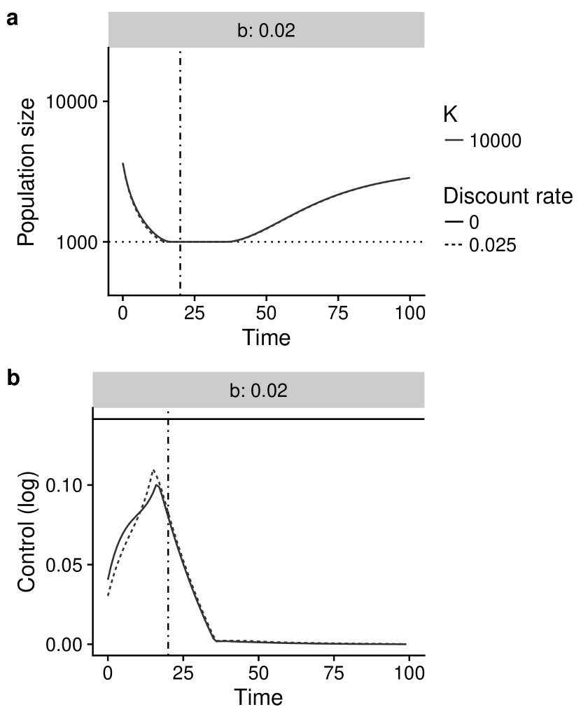
Figure 4: Optimal control with varying discount rate (varying linetype) including zero discount. The zero-discount path was used to initialize the runs with positive discount. (a) Population sizes under the optimal path of investment in intervention, which includes the constraint of not allowing the population to fall below a size considered vulnerable to extinction (horizontal dotted line). (b) Optimal investment trajectory relative to the budget constraint (horizontal line). All solutions assume decelerating environmental change as in Figure 1a where the rate of environmental change decreases to the critical rate where evolutionary rescue can occur at $t_{\text{safe}}$ (vertical dash-dot line).

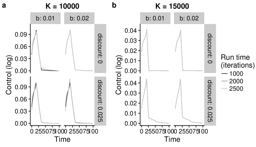
Figure 5: Optimal paths for increasing run times (lighter greys) to show convergence of control paths for different budgets (columns) and discount rates (subpanel rows) at three carrying capacities corresponding to (a) $K=10,000$, (b) $K=15,000$. There are three runs shown in each panel: 1000, 2000, and 2500 iterations. In most cases the two longest runs resulted in the same path.

Figure 6: Optimal paths for increasing run times (lighter greys) to show convergence of population trajectories for different budgets (columns) and discount rates (subpanel rows) at three carrying capacities corresponding to (a) $K=10,000$, (b) $K=15,000$. There are three runs shown in each panel: 1000, 2000, and 2500 iterations. In most cases the two longest runs resulted in the same path.