On the time evolution of fermionic occupation numbers

Abstract

We derive an equation for the time evolution of the natural occupation numbers for fermionic systems with more than two electrons. The evolution of such numbers is connected with the symmetry-adapted generalized Pauli exclusion principle, as well as with the evolution of the natural orbitals and a set of many-body relative phases. We then relate the evolution of these phases to a geometrical and a dynamical term, attached to each one of the Slater determinants appearing in the configuration-interaction expansion of the wave function.

I Introduction

The time evolution of an electronic system is governed by the Schrödinger equation Schrödinger (1926). Yet a real-time propagation of the many-fermion wave function is, by and large, computationally prohibitive. The time-dependent extension of density functional theory (TDDFT) alleviates this computational problem by mapping the evolution of the ground-state density to the one of a certain auxiliary system Runge and Gross (1984). Since such auxiliary system is non-interacting, TDDFT does not involve fractional occupation numbers, which are at any rate important for capturing quantum correlations Appel and Gross (2010); Lackner et al. (2015), even in the adiabatic regime Requist and Pankratov (2010).

It is well known that the ground-state wave function of an electronic system can be written as a functional of the one-body reduced density matrix, which for a wave function $\Psi$ is defined as

$$\gamma(1,1^{\prime})\equiv\mbox{$\langle\Psi|$}\hat{\psi}^{\dagger}(1^{\prime})\hat{\psi}(1)\mbox{$|\Psi\rangle$},$$ (1)

with the short notation $1\equiv(\bm{r}_{1},\varsigma_{1})$ for position and spin coordinates. Thus, ground states can be viewed as functionals of such reduced densities (say, $\Psi_{\rm gs}[\gamma]$) Gilbert (1975). Since $\gamma$ accounts for fractional natural occupation numbers (i.e., its eigenvalues), employing this matrix as the main object leads to a theory able to capture quite well strong (static) electron correlations Cohen, Mori-Sánchez, and Yang (2008a, b); Benavides-Riveros, Lathiotakis, and Marques (2017); Schade, Kamil, and Blöchl (2017). For instance, unlike density functional theory, such a density-matrix functional theory correctly predicts the insulating behavior of Mott-type insulators Sharma et al. (2013); Pernal (2015). Furthermore, it has been recently pointed out that $\gamma$ encodes essential many-body aspects of interacting fermions and hard-core bosons, as many-body localization transitions Bera et al. (2015); Lezama et al. (2017), entanglement Walter et al. (2013); Maciążek and Sawicki (2018), or topological states He et al. (2017). Given these remarkable properties, there is a growing interest in proposing protocols to access to the structure of this density matrix both experimentally using quantum-gas microscopes Peña Ardila, Heyl, and Eckardt (2018), or theoretically employing quantum computers Smart, Schuster, and Mazziotti (2019) and hard-core bosons Tennie, Vedral, and Schilling (2017a).

Unfortunately, time-dependent extensions of the theory of the one-body reduced density matrix suffer from various shortcomings. Save for two-electron systems, the current status of the theory does not allow the fermionic occupation numbers to evolve in time Pernal, Gritsenko, and Baerends (2007); Giesbertz, Baerends, and Gritsenko (2008); van Meer, Gritsenko, and Baerends (2017); Giesbertz, Gritsenko, and Baerends (2010a). To understand the problem it is worth recalling that the Schrödinger equation leads to the BBGKY hierarchy, whose equation for $\gamma(t)$ is Bonitz (1998):

$$i\frac{d\hat{\gamma}(t)}{dt}=[\hat{h}(t),\hat{\gamma}(t)]+\hat{u}(t),$$ (2)

where $\hat{h}(t)$ is the time-dependent one-particle Hamiltonian operator and $\hat{u}(t)$ is in spatial and spin representation $u(1,1^{\prime},t)=2\int[v(1,2)-v(1^{\prime},2)]\Gamma(1,2;1^{\prime},2,t)d2$. $v(1,2)$ is the Coulomb potential and $\Gamma(1,2;1^{\prime},2^{\prime},t)$ is the two-particle reduced density matrix. The density matrix $\hat{\gamma}(t)$ could also be computed by integrating out $\Gamma(t)$ which satisfies in turn an equation similar to (2). Since the representability conditions of the three-particle reduced density matrix $\Gamma_{3}$ are much harder to implement, this latter procedure is not completely well-defined: the positive-semidefiniteness of $\Gamma_{3}$ is not necessarily inherited by $\Gamma$ and $\gamma$, neither the energy is conserved in the absence of time-dependent potentials Akbari et al. (2012). For this reason, it is believed that fermionic constraints on the occupation numbers should play a role in implementing the BBGKY hierarchy Lackner et al. (2015).

By definition, in the natural-orbital basis $\hat{\gamma}(t)$ is diagonal, reading

$$\hat{\gamma}(t)=\sum_{k}n_{k}(t)\mbox{$|\varphi_{k}(t)\rangle$}\mbox{$\langle\varphi_{k}(t)|$}.$$ (3)

By multiplying Eq. (2) by $\varphi^{*}_{j}(1)$ and $\varphi_{k}(1^{\prime})$, and integrating both position and spin coordinates, Pernal, Gritsenko and Baerends obtained an equation for the time-evolution for the natural orbitals Pernal, Gritsenko, and Baerends (2007), namely,

$$i\mbox{$\langle\varphi_{j}|$}\dot{\varphi}_{k}\rangle=\mbox{$\langle\varphi_{j}|$}\hat{h}\mbox{$|\varphi_{k}\rangle$}+\frac{W_{jk}-W_{kj}^{*}}{n_{k}-n_{j}},\qquad j\neq k$$ (4)

as well as an equation for the time evolution of the natural occupation numbers:

$$\dot{n}_{k}=2\Im[W_{kk}],$$ (5)

where $W_{jk}\equiv 2\int v(1,2)\Gamma(1,2;1^{\prime},2)\varphi^{*}_{j}(1)\varphi_{k}(1^{\prime})d1d1^{\prime}d2$. The presence of the difference $(n_{k}-n_{j})$ in Eq. (4) indicates that degeneracies of the occupations lead to singularities in the time evolution of the natural orbitals. It is not a surprise, since degenerancy of the occupation numbers implies an ambiguity in the definition of the corresponding natural orbitals (for a linear combination of degenerate natural orbitals is also a natural orbital). For simplicity, it is in general assumed the absence of such a degenerancy. Since the imaginary part of $W_{kk}$ determines the time evolution of the occupations (5), it is clear that some relative phases are crucial to correctly capture the dynamics of the system. With the exception of the Löwdin-Shull functional for two-electron systems Löwdin and Shull (1956), the PNOF4 functional for density-matrix functional theory Piris (2013), and its latter developments Mitxelena, Rodriguez-Mayorga, and Piris (2018), the right-hand of Eq. (5) vanishes identically for current reconstructions of $\Gamma$ in terms of $\gamma$, so the occupation numbers do not evolve in time Pernal and Giesbertz (2016). There are a few attempts in the literature to account for relative phases at the level of the two-body reduced density matrix. Yet, the theory developed in this way is limited to the two-electron case Giesbertz, Gritsenko, and Baerends (2010b, 2012); Requist and Pankratov (2011); Rapp, Brics, and Bauer (2014). By studying the underlying exchange symmetry, this paper is aimed at proposing a new way of tackling the time dependency of the natural occupation numbers of fermionic systems. By doing so, we present an approximative formula for the adiabatic time evolution of the occupation numbers for fermionic systems.

Besides this introduction, the paper contains three additional parts. In Sec. II we discuss the so-called generalized Pauli constraints and how they can help us to extract information of the wave function. In Sec. III, we present a couple of formulas for the time evolution of a pinned system of three electrons in six natural orbitals. By exploiting the information of symmetries, Sec. IV generalizes this result for larger systems. The paper ends with a conclusion section and three appendices.

II Robustness of fermionic constraints

To first shed light into this problem we study the evolution of the one-body reduced density matrix for pinned wave functions, which, as we will show, are structural simplifications of some ground states. From a formal viewpoint, it is known that the compatibility, or representability, of a fermionic one-body reduced density matrix $\gamma$ with respect to a quantum many-body state $|\Psi\rangle$ is described by sets of linear constraints on its spectra $\bm{n}\equiv(n_{1},n_{2},\dots)$, namely Klyachko (2006); Altunbulak and Klyachko (2008):

$$\mathcal{D}_{j}(\bm{n})\equiv\kappa_{j}^{0}+\sum_{i}\kappa_{j}^{i}n_{i}\geq 0,$$ (6)

where the coefficients $\kappa_{j}^{i}$ are integers depending on the number of fermions $N$ and the dimension of the underlying one-particle Hilbert space $M$. Along with the non-increasing ordering of the natural occupation numbers (say, $n_{i}\geq n_{i+1}$) and the sum rule ($\sum_{i}n_{i}=N$), these generalized Pauli constraints (6) define a polytope where the sets of $\bm{n}$, which are compatible with $N$-fermion pure states, lie Sawicki, Oszmaniec, and Kuś (2014). It is quite remarkable that, whenever some of those quantum marginal constraints are saturated or pinned, the total quantum state has a specific, simplified structure. Indeed, $\mathcal{D}_{j}(\bm{n})=0\Longleftrightarrow\hat{D}_{j}\mbox{$|\Psi\rangle$}=0$, where the operator $\hat{D}_{j}=\kappa_{j}^{0}+\sum_{i}\kappa_{j}^{i}\hat{n}_{i}$ is built by replacing the occupation numbers in Eq. (6) by the corresponding particle number operators. The importance of this result lies on the fact that it provides an important selection rule for the Slater determinants that can appear in the configuration-interaction expansion of wave functions Benavides-Riveros and Schilling (2016). Indeed, a wave function whose spectrum is pinned to one of the polytope’s facets $\mathcal{P}_{j}=\{\bm{n}|\mathcal{D}_{j}(\bm{n})=0\}$ (see Fig. 1) can be written as a linear superposition of the Slater determinants which belong to the zero-eigenspace of the operator $\hat{D}_{j}$. This selection rule can be used to systematically produce ansätzen for ground states in the form of sparse wave functions, which, instead of using the full Hilbert space, can be expanded in the basis of the natural orbitals (the eigenvalues of $\gamma$) with a few Slater determinants Benavides-Riveros and Schilling (2016); Chakraborty and Mazziotti (2018). Apart from the simplification of the wave function, there is another advantage in using natural orbitals that is worth mentioning here: it is known that the basis of natural orbitals is typically quite good to convergence the full wave function.

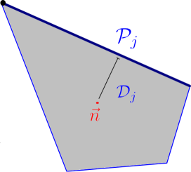
Figure 1: Illustration of the distance $\mathcal{D}_{j}$ of $\bm{n}$ to the polytope facet $\mathcal{P}_{j}$.

This structural simplification for pinned quantum systems is stable in the sense that any many-fermion quantum state can be approximated by the structural simplified form corresponding to saturation of the generalized Pauli constraint $\mathcal{D}_{j}$. The error of such a simplification is bounded by twice the distance of the vector of its occupation numbers to the corresponding polytope’s facet $\mathcal{P}_{j}$ Schilling, Benavides-Riveros, and Vrana (2017). Recently, it has been suggested that the generalized Pauli constraints may facilitate the development of more accurate functionals within density-matrix functional theory Benavides-Riveros and Marques (2018); Schilling (2018); Schilling and Schilling (2019). Since quasipinning (say, $\mathcal{D}_{j}(\bm{n})\approx 0$) is approximately observed for several ground states, the quasipinning “mechanism” has attracted some attention in quantum chemistry and quantum-information theory Schilling (2014); Benavides-Riveros (2018); Schilling, Gross, and Christandl (2013); Benavides-Riveros, Gracia-Bondia, and Springborg (2013); Schilling (2015); Chakraborty and Mazziotti (2014, 2015); Benavides-Riveros and Springborg (2015); Theophilou et al. (2015); Mazziotti (2016); Tennie et al. (2016); Tennie, Vedral, and Schilling (2016); DePrince (2016); Tennie, Vedral, and Schilling (2017b); Benavides-Riveros et al. (2017); Schilling et al. (2018); Requist and Gross (2018).

It can also be shown that the structural simplification of the wave function is also stable in the sense that pinning is robust under any small perturbation of the Hamiltonian. Klyachko has indeed suggested that a pinned system should remain so under a reasonably small variation of the Hamiltonian Klyachko (2009). This can be easily seen by perturbing a Hamiltonian $\hat{H}$ with non-degenerated eigenstates $|\Psi_{n}\rangle$ and eigenenergies $E_{n}$. In perturbation theory the ground state of the perturbed Hamiltonian $\hat{H}(\lambda)\equiv\hat{H}+\lambda\hat{V}$ reads as $\mbox{$|\Psi^{\lambda}_{0}\rangle$}=\mbox{$|\Psi_{0}\rangle$}-\lambda\sum_{n\neq 0}b_{n}\mbox{$|\Psi_{n}\rangle$}+\mathcal{O}(\lambda^{2})$, with $b_{n}=\mbox{$\langle\Psi_{n}|$}\hat{V}\mbox{$|\Psi_{0}\rangle$}/(E_{n}-E_{0})$. If the unperturbed ground state is pinned to a facet $\mathcal{P}_{j}$, then $\hat{D}_{j}\mbox{$|\Psi_{0}\rangle$}=0$, and therefore, the perturbed distance to that polytope’s facet reads now as ${\mathcal{D}}_{j}(n^{\lambda}_{0})=\mbox{$\langle\Psi^{\lambda}_{0}|$}\hat{D}_{j}\mbox{$|\Psi^{\lambda}_{0}\rangle$}\sim\mathcal{O}(\lambda^{2})$. Based on a self-consistent perturbation theory, it has also been shown that a perturbation of a one-particle Hamiltonian (whose ground state is a Slater determinant) induces a change in pinning only in second order Legeza and Schilling (2018). Those results are somehow expected, since the expectation value of any symmetry $\hat{\mathfrak{s}}$ satisfied by a (non-degenerated) ground state remains constant in first-order pertubation theory. Indeed,

$$\mbox{$\langle\Psi^{\lambda}_{0}|$}\hat{\mathfrak{s}}\mbox{$|\Psi^{\lambda}_{0}\rangle$}=\mbox{$\langle\Psi_{0}|$}\hat{\mathfrak{s}}\mbox{$|\Psi_{0}\rangle$}+\mathcal{O}(\lambda^{2}).$$ (7)

This immediately implies that whenever the (non-degenerated) ground state of a system belongs eigenspace of a given symmetry operator, it remains in such an eigenspace in first order upon perturbation. For instance, as is well known, a system which is pinned to the Pauli exclusion principle (say, a occupancy is equal to 1 or 0) stay so in the first order of the perturbation.

Remarkably the same is approximately true for quasipinning. In Appendix A we show that the response of quasipinning under a perturbation is bounded from above by the formula:

$$\mathcal{D}_{j}(\bm{n}^{\lambda}_{0})\leq\mathcal{D}_{j}(\bm{n}_{0})+2\lambda\gamma_{V}\sqrt{\langle\hat{D}^{2}_{j}\rangle}+\mathcal{O}(\lambda^{2}),$$ (8)

where $\langle\hat{D}^{2}_{j}\rangle=\mbox{$\langle\Psi_{0}|$}\hat{D}^{2}_{j}\mbox{$|\Psi_{0}\rangle$}$. The multiplicative prefactor $\gamma_{V}$ is a relative strength between the perturbation and the unperturbed Hamiltonian. This strength can be further bounded (see Appendix A):

$$\gamma_{V}\leq\frac{\sqrt{{\rm Cov}_{\Psi_{0}}(\hat{V})}}{E_{\rm gap}},$$ (9)

where the energy gap is defined as the difference between the first-excited and ground-state energies $E_{\rm gap}=E_{1}-E_{0}$, and the covariance of the perturbation is ${\rm Cov}_{\Psi_{0}}(\hat{V})=\mbox{$\langle\Psi_{0}|$}\hat{V}^{2}\mbox{$|\Psi_{0}\rangle$}-\mbox{$\langle\Psi_{0}|$}\hat{V}\mbox{$|\Psi_{0}\rangle$}^{2}$.

The appearance of the term $\langle\hat{D}_{j}^{2}\rangle$ in (8) indicates that, in order to predict the stability of quasipinned systems, the expected value of the square of the operator $\hat{D}_{j}$ deserves further attention in quasipinning theory. It is worth noticing that, when the system is pinned, $\langle\hat{D}^{2}_{j}\rangle=0$, and therefore the pinning response goes only in second order, as Klyachko correctly stressed. In a more general fashion, paraphrasing Klyachko, we have shown that since a quasipinned system is approximately driven by Pauli kinematics, it should remain approximately pinned to that facet under a reasonably small variation of the Hamiltonian, as long as $\langle\hat{D}_{j}^{2}\rangle$ is also small.

III A formula for the time evolution of the fermionic occupation numbers

This robustness of (quasi)pinning prompts us to seek for the equation of motion of the one-body reduced density matrix of a pinned quantum system. Geometrically, the aim is to constrain the dynamics of the system to move on a hyperplane in the one-particle picture. To illustrate our approach let us consider the so-called Borland-Dennis wave function, namely, the pinned rank-six approximation (i.e., $M=6$) for the three-active-electron system Borland and Dennis (1972). This wave function is known to be pinned to one of the facets of the corresponding polytope (i.e., $n_{1}+n_{2}+n_{4}=2$) and can be written explicitly in terms of the amplitude squares $f_{\alpha}$, the natural orbitals $\varphi_{\alpha}$ (whose time derivative is defined by Eq. (4)) and the relative phases $\xi_{\alpha}$. It reads:

$$\mbox{$|\Phi_{\rm BD}[\bm{f},\bm{\varphi},\bm{\xi}]\rangle$}=\sum_{\alpha}\sqrt{f_{\alpha}}e^{-i\xi_{\alpha}}\mbox{$|\bm{\varphi_{\alpha}}\rangle$},$$ (10)

where $|\cdot\rangle$ denotes normalized Slater determinants. The coefficient $\alpha\in\{3,5,6\}$, and $\bm{\varphi_{3}}(t)\equiv\varphi_{1}(t)\varphi_{2}(t)\varphi_{3}(t)$, $\bm{\varphi_{5}}(t)\equiv\varphi_{1}(t)\varphi_{4}(t)\varphi_{5}(t)$ and $\bm{\varphi_{6}}(t)\equiv\varphi_{2}(t)\varphi_{4}(t)\varphi_{6}(t)$. In the Borland-Dennis state (10) the square of the amplitudes $\bm{f}$ turn out to be equal to three occupation numbers. This trivial correspondence between $\bm{n}$ and $\bm{f}$ will be crucial to later generalize our results. For the wave function (10) there are other three saturated generalized Pauli constraints, namely, $n_{k}+n_{7-k}=1$ with $k\in\{1,2,3\}$. We will exploit later the well-known fact that the relative phases $\xi_{\alpha}$ can only be uniquely defined with respect to a given choice of the time-dependent phases of the natural orbitals Requist and Pankratov (2011).

Recall that the time evolution of the natural orbitals is completely determined by the off-diagonal terms $\mbox{$\langle\varphi_{j}|$}\partial_{t}\varphi_{k}\rangle$ $(j\neq k)$ in Eq. (4). The expression for the two-particle reduced density matrix can be easily found by tracing out 1 particle from the full density matrix: $\Gamma=3{\rm Tr}_{1}[\mbox{$|\Phi_{\rm BD}\rangle$}\mbox{$\langle\Phi_{\rm BD}|$}]$. The missed diagonal terms $\mbox{$\langle\varphi_{k}|$}\dot{\varphi}_{k}\rangle$ can be removed as convenient phase factors Schmelcher, Krönke, and Diakonos (2017) (see below). The equations of motion of $\bm{\xi}$ and $\bm{f}$ can be derived from the stationary condition of the time-dependent quantum mechanical action

$$\mathcal{A}_{\Psi}(t_{1},t_{2})=\int_{t_{1}}^{t_{2}}\mbox{$\langle\Psi(\tau)|$}i\partial_{\tau}-\hat{H}(\tau)\mbox{$|\Psi(\tau)\rangle$}d\tau.$$ (11)

That this action gives place to the Schrödinger operator can be easily seen by variating $\mathcal{A}_{\Psi}$ with respect to the state $\langle\Psi(t)|$ under the constraint of norm conservation Löwdin and Mukherjee (1972). $\mathcal{A}_{\Psi}$ is therefore stationary for the correct state $|\Psi(t)\rangle$ which develops from a given initial state $|\Psi(t_{1})\rangle$. By optimizing the functional $\mathcal{A}_{\Phi_{\rm BD}}$ with respect to the phases, one obtains an explicit equation for the evolution of the square amplitudes.

The time derivative of the Borland-Dennis wave function (10) gives $\mbox{$\langle\Phi_{\rm BD}|$}i\partial_{t}\mbox{$|\Phi_{\rm BD}\rangle$}=\sum_{\alpha}f_{\alpha}(\dot{\xi}_{\alpha}+\mbox{$\langle\bm{\varphi_{\alpha}}|$}i\partial_{t}\mbox{$|\bm{\varphi_{\alpha}}\rangle$})$. We have used the fact that $\sum_{\alpha}\dot{f}_{\alpha}=0$ and $\mbox{$\langle\bm{\varphi_{\beta}}|$}\partial_{t}\mbox{$|\bm{\varphi_{\alpha}}\rangle$}=0$ for $\beta\neq\alpha$, because two different Slater determinants in Eq. (10) differ by at least two orbitals. The expected value of the Hamiltonian is:

$$\mbox{$\langle\Phi_{\rm BD}|$}\hat{H}\mbox{$|\Phi_{\rm BD}\rangle$}=\sum_{\alpha\beta}\sqrt{f_{\alpha}f_{\beta}}e^{i(\xi_{\beta}-\xi_{\alpha})}\mbox{$\langle\bm{\varphi_{\beta}}|$}\hat{H}\mbox{$|\bm{\varphi_{\alpha}}\rangle$}.$$ (12)

Optimizing the functional $\mathcal{A}[\Phi_{\rm BD}]$ with respect to the phases gives the following equation of motion:

$$i\dot{f}_{\alpha}=\sum_{\beta\neq\alpha}\sqrt{f_{\alpha}f_{\beta}}\left[\mbox{$\langle\bm{\varphi_{\beta}}|$}\hat{H}\mbox{$|\bm{\varphi_{\alpha}}\rangle$}e^{i(\xi_{\beta}-\xi_{\alpha})}-{\rm c.c.}\right].$$ (13)

To complete the time-evolution picture of the quantum system we need equations for the evolution of the relative phases $\bm{\xi}$, which can be derived from the stationary condition of the action $\mathcal{A}[\Phi_{\rm BD}]$ with respect to $\bm{f}$. The evolution of the relative phases is determined by the instructive relation:

$$\xi_{\alpha}(t)=\xi_{\alpha}^{\rm geo}(t)+\xi^{\rm dyn}_{\alpha}(t).$$ (14)

This result relates the evolution of the phases with a Slater-geometrical phase

$$\xi_{\alpha}^{\rm geo}(t)=-i\int_{0}^{t}\langle\bm{\varphi_{\alpha}}|\partial_{\tau}\mbox{$|\bm{\varphi_{\alpha}}\rangle$}d\tau$$ (15)

attached to the Slater determinant $|\bm{\varphi_{\alpha}}\rangle$, and an additional Slater-dynamical phase which is written in terms of the diagonal and non-diagonal elements of the Hamiltonian driving the dynamics of the system, namely,

$$\xi^{\rm dyn}_{\alpha}(t)=\int_{0}^{t}\sum_{\beta}\frac{1}{2}\sqrt{\frac{f_{\beta}}{f_{\alpha}}}\left[\mbox{$\langle\bm{\varphi_{\alpha}}|$}\hat{H}\mbox{$|\bm{\varphi_{\beta}}\rangle$}e^{i(\xi_{\alpha}-\xi_{\beta})}+{\rm c.c.}\right]d\tau.$$ (16)

Notice that the Slater-geometrical phase $\xi_{\alpha}^{\rm geo}(t)$ contains the missing diagonal terms of Eq. (4). This phase indicates clearly that the natural orbitals should be shifted accordingly. To see that let us define the phase-shifted natural orbitals

$$\mbox{$|\tilde{\varphi}_{k}\rangle$}=e^{-\int_{0}^{t}\mbox{$\langle\varphi_{k}|$}\partial_{\tau}\mbox{$|\varphi_{k}\rangle$}d\tau}\mbox{$|\varphi_{k}\rangle$}.$$ (17)

By construction (see Appendix B), we have $\mbox{$\langle\tilde{\varphi}_{k}|$}\tilde{\varphi}_{l}\rangle=\delta_{k}^{l}$ and in particular $\mbox{$\langle\tilde{\varphi}_{k}|$}\partial_{t}\mbox{$|\tilde{\varphi}_{k}\rangle$}=0$, which means that the derivative $\partial_{t}\mbox{$|\tilde{\varphi}_{k}\rangle$}$ is perpendicular to $|\tilde{\varphi}_{k}\rangle$. This is the parallel-transport well-known condition. In turn, Slater determinants satisfy

$$\mbox{$|\bm{\varphi}_{\alpha}\rangle$}=e^{i\xi^{\rm geo}_{\alpha}}\mbox{$|\bm{\tilde{\varphi}}_{\alpha}\rangle$},$$ (18)

which is a parallel-transport condition for Slater determinants. Notice the different sign in front of the phases in Eq. (18) and Eq. (10). Therefore, in the basis of phase-shifted natural orbitals, the Slater-geometrical phase does not contribute to the time evolution of the natural occupation numbers. We can now rewrite our results in terms of $|\bm{\tilde{\varphi}}_{\alpha}\rangle$: formulas (13) and (16) change just by replacing $\mbox{$|\bm{\varphi}_{\alpha}\rangle$}\rightarrow\mbox{$|\bm{\tilde{\varphi}}_{\alpha}\rangle$}$ and $\xi_{\alpha}(t)\rightarrow\xi^{\rm dyn}_{\alpha}(t)$. Since the seminal paper of Berry Berry (1984), this kind of phases has been discovered in many fields of physics Aharonov and Anandan (1987); Resta (1998); Xiao, Chang, and Niu (2010); Requist, Tandetzky, and Gross (2016). Yet the result (16) is unique in establishing a direct relationship for fermionic systems between Slater determinants and the dynamical phases. Moreover, since the wave function and the Slater determinants are written in terms of the natural orbitals and the occupation numbers, the phases presented here are functions of one-body reduced quantities (say, $\xi_{\alpha}^{\rm dyn}[\gamma,\bm{\xi}^{\rm dyn}]$). We emphasize that Eq. (16) is absent from the standard formulation of time-dependent density-matrix functional theory, and this is the reason for its severe shortcomings. Notice also that the result (16) can be easily generalized to any natural orbital that appears in one and only one of the Slater determinants in the configuration-interaction expansion of the wave function (this is the argument for the two-electron system Giesbertz, Gritsenko, and Baerends (2012)). In addition, it is remarkable that the relative dynamical phases retain the memory effects of the system’s time evolution.

Before finishing this section, it is worth recalling that some ground states are very close to, but not exactly on, one of the boundaries of the polytope. For quasipinned systems we use as an ansatz a pinned wave function. Therefore, by restricting the evolution to one of the hyperplanes in the one-particle picture, we are able to unveil an approximate equation for the evolution of the occupation numbers for a three-electron system.

IV Generalization

To generalize our results let us consider translationally invariant systems on a one-band lattice with periodic boundary conditions. Let us consider, for instance, the Hubbard model with periodic boundary conditions. The magnetization $m$ and the total Bloch number $T$ are good quantum numbers. The Hamiltonian is block diagonal with respect to those symmetries (and other ones like the total spin or the parity). Clearly, the representability conditions for each symmetry sector are more restrictive than the generalized Pauli exclusion principle, but the computation of the former constraints is considerably simpler than the calculation of the latter ones. This is the symmetry-adapted generalized Pauli exclusion principle, which we now exploit. To distinguish both types of generalized Pauli constraints, let us call $d^{s}_{j}(\bm{n})$ the ones coming from a symmetry-adapted sector $s$.

Due to translational and spin symmetries, any two Slater determinants belonging to the same symmetry sector should differ by at least two natural orbitals Schilling and Schilling (2019). It is a consequence of these symmetries that the corresponding one-body reduced density matrix is diagonal. This kind of wave functions are used in quantum-computing simulations of quantum chemistry models Babbush et al. (2015). Another important example of these wave functions is the seniority-zero sector of the Hilbert space for even-number of electrons Bytautas et al. (2011). It has also been shown that writing the wavefunction in the basis of natural orbitals leads to a sharp drop of the coefficients of Slater determinants containing just single or triple excitations Mentel et al. (2014) which can also be argued by using pinning arguments for general systems Benavides-Riveros and Springborg (2015).

The wave function reads exactly as (10) but $\alpha$ stands now for a string of numbers indexing the natural orbitals in lexicographic order (e.g, $\mbox{$|\bm{\varphi}_{123}\rangle$}=\mbox{$|\varphi_{1}\varphi_{2}\varphi_{3}\rangle$}$). The amplitudes $f_{\alpha}$ can be related with the natural occupation numbers by a linear transformation, $\mathcal{M}^{s}_{(N,M)}\bm{f}=\bm{n}$. The crucial observation is that, whenever there are as many Slater determinants as independent occupation numbers, the matrix $\mathcal{M}^{s}_{(N,M)}$ is invertible Schilling and Schilling (2019). Its inverse is a matrix of integers (up to a global normalization constant) whose entries depend on $(N,M)$ and the corresponding symmetry sector. To give an example, consider the Hubbard model with three spin-$\tfrac{1}{2}$ fermions on four lattice sites. For such a system, there are 31 $N$-representability conditions. Yet, after restricting to some symmetry sector, the number of such constraints is much smaller. Consider in particular the sector $(m,T)=(\tfrac{1}{2},1)$. This is a six dimensional Hilbert space and, as shown in the Appendix C, there are six symmetry-preserving constraints, which can be written as a linear superposition of the independent occupation numbers:

$$d^{s}_{j}(\bm{n})=\frac{1}{4}\sum^{2}_{i=0}\left(\kappa^{j}_{i\uparrow}n_{i\uparrow}+\kappa^{j}_{i\downarrow}n_{i\downarrow}\right),$$ (19)

where $\kappa_{i\sigma}^{j}$ are integers. In addition, we have the simpler spin constraints $\sum_{i=0}^{3}n_{i\uparrow}=2$ and $\sum_{i=0}^{3}n_{i\downarrow}=1$.

A more elementary example is the traslationally invariant version of the Borland-Dennis setting (i.e., the Hilbert space $(N,M)=(3,6)$: $\mathcal{H}={\rm span}\{\mbox{$|\bm{\varphi}_{123}\rangle$},\mbox{$|\bm{\varphi}_{145}\rangle$},\mbox{$|\bm{\varphi}_{246}\rangle$},\mbox{$|\bm{\varphi}_{356}\rangle$}\})$ whose symmetry-preserving constraints can be easily computed. Indeed, $f_{123}=\tfrac{1}{2}(n_{1}+n_{2}+n_{3}-1)$, $f_{145}=\tfrac{1}{2}(n_{1}-n_{2}+1-n_{3})$, and $f_{246}=\tfrac{1}{2}(1-n_{1}+n_{2}-n_{3})$. One can recognize in $f_{356}=\tfrac{1}{2}(1-n_{1}-n_{2}+n_{3})=\tfrac{1}{2}(2-n_{1}-n_{2}-n_{4})$ the famous Borland-Dennis representability condition for three-fermions in a six dimensional one-particle Hilbert space, safe a normalization constant. Therefore, in this case we can make use of the generalized Pauli principle by writing $f_{356}=\tfrac{1}{2}\mathcal{D}(\bm{n})$. This is nothing more than the constraint that we have saturated (i.e., $2-n_{1}-n_{2}-n_{4}=0$) in Sec. (III). The other fermionic constraints $d^{s}_{\alpha}({\bm{n}})\equiv f_{\alpha}(\bm{n})$ are just sophisticated versions of the (normal) Pauli exclusion principle $0\leq n_{i}\leq 1$, plus the ordering $n_{i}\geq n_{i+1}$. Notice in passing that in this example all the constraints can be rewritten as

$$f_{ijk}=\tfrac{1}{2}(n_{i}+n_{j}+n_{k}-1),$$ (20)

which shows that each one of these fermionic constraints measures the distance (normalized to 1) to the opposite facet to the polytope’s vertex $n_{i}=n_{j}=n_{k}=1$, and $n_{l}=0$ if $l\notin\{i,j,k\}$. For example, $f_{356}$ measures the distance to the non-elementary facet $2=n_{1}+n_{2}+n_{4}$. A similar reasoning holds for the constraints of the former example of three $\tfrac{1}{2}$-fermions in four lattice sides $(3,4)$. We believe that this geometrical picture of the time evolution of the occupation numbers and the fermionic constraints indicates a promising future research path.

By means of the inversion of $\bm{n}=\mathcal{M}^{s}_{(N,M)}\bm{f}$, we can now assign square amplitudes to constraints in a meaningful way (i.e, $f_{\alpha}=d^{s}_{\alpha}(\bm{n})$). This last relation is exact at $t=0$. Since the natural orbitals retain their orthonormality through the whole system’s time evolution, it is also exact instantaneously. Therefore, by employing the results of the last section, in particular Eq. (13), the time-evolution of the natural occupation numbers is thus given by:

$$\dot{\bm{n}}=\mathcal{M}^{s}_{(N,M)}\dot{\bm{f}},$$ (21)

where

$$i\dot{f}_{\alpha}=\sum_{\beta\neq\alpha}\sqrt{d^{s}_{\alpha}(\bm{n})d^{s}_{\beta}(\bm{n})}\left[\mbox{$\langle\tilde{\bm{\varphi}}_{\beta}|$}\hat{H}\mbox{$|\tilde{\bm{\varphi}}_{\alpha}\rangle$}e^{i(\xi^{\rm dyn}_{\beta}-\xi^{\rm dyn}_{\alpha})}-{\rm c.c.}\right].$$ (22)

The dynamical phase $\xi^{\rm dyn}_{\alpha}(t)$ is given by the Eq. (16), making again the substitution $f_{\alpha}=d^{s}_{\alpha}(\bm{n})$:

$$\xi^{\rm dyn}_{\alpha}(t)=\int_{0}^{t}\sum_{\beta}\frac{1}{2}\sqrt{\frac{d^{s}_{\beta}(\bm{n})}{d^{s}_{\alpha}(\bm{n})}}\left[\mbox{$\langle\tilde{\bm{\varphi}}_{\alpha}|$}\hat{H}\mbox{$|\tilde{\bm{\varphi}}_{\beta}\rangle$}e^{i(\xi^{\rm dyn}_{\alpha}-\xi^{\rm dyn}_{\beta})}+{\rm c.c.}\right]d\tau.$$ (23)

In the case of the Hubbard model with three spin-${\tfrac{1}{2}}$ fermions on four lattice sites, the evolving occupation numbers $n_{l\sigma}(t)$ lost the connection with the orbital $\tilde{\varphi}_{l\sigma}$ as soon as the perturbation is switched on. Yet $n_{l\sigma}(t)$ is defined as the occupation number associated with the time evolving natural orbital $\tilde{\varphi}_{l\sigma}(t)$, such that $\tilde{\varphi}_{l\sigma}(0^{+})=\tilde{\varphi}_{l\sigma}$ and $n_{l\sigma}(0^{+})=n_{l\sigma}$.

These three last equations are the main results of this paper. The time-evolution picture is then as follows. From the BBGKY hierarchy one can obtain Eq. (4) for the time evolution of the (phase-shifted) natural orbitals. From the time-dependent quantum mechanical action we obtained the equation of motion of the square amplitudes (22) and the relative phases (23). By exploiting generalized Pauli constraints (in a given symmetry sector) we have found Eq. (21) and its corresponding inversion for the time evolution of the natural occupation numbers. All the equations are written in terms of one-particle quantities (i.e., occupation numbers and natural orbitals) plus a set of supplementary dynamical phases (as many as independent occupation numbers), which retain the memory effects of the system.

Four key observations are in order here. First, the phases $\bm{\xi}$ are not attached to the natural orbitals in the sense of the so-called phase-included natural orbital theory Giesbertz, Gritsenko, and Baerends (2010a), and therefore our expressions go well beyond the realm of two-electron systems. Second, Eqs. (21) and (22) can be understood as the time-evolution of the recently discovered density-matrix functional for translationally invariant systems with periodic boundary conditions Schilling and Schilling (2019). The divergence ($1/\sqrt{D_{\alpha}(\bm{n})}$) observed in such a functional at the level of ground states is also observed here at the level of the dynamical phase for time evolving systems. Third, it is expected that Eqs. (21) and (22) are a reasonable approximation for the time evolution of molecular systems, because the contribution of single (and more generally odd) excitations in the configuration-interaction expansion in the natural-orbital basis tends to be negligible Mentel et al. (2014); Benavides-Riveros and Springborg (2015). Finally, it is always possible that even after recognizing of the symmetries satisfied by the ground (or initial) state the number of Slater determinants exceeds the number of natural orbitals. In that case one can always use the structural simplification due to pinning to reduced the dimensionality of the Hilbert space, or to resort to more involve “inversion” techniques Legeza and Schilling (2018).

V Conclusions

Describing the dynamics of strongly driven electron dynamics is a challenging problem. Multiconfigurational wave functions with enough terms to adequately describe correlation have so far been limited to small systems or short simulation times. In this paper we investigated the time evolution of the one-body reduced density matrix, based on recent progress on fermionic exchange symmetry for pure systems. In particular, we have employed the stability (under any small perturbation of the Hamiltonian) of the structural simplification of the wave function due to quasipinning or, more generally, symmetries. We presented two important results. First, we developed a closed expression for the time evolution of fermionic natural occupation. This evolution depends on one-particle quantities (the natural orbitals and the occupation numbers themselves) as well as to a set of dynamical phases. Second, we have presented a formula for the evolution of such dynamical phases. We believe that this last equation is the missing piece for the successful application of reduced density-matrix functional theory to time-dependent problems. Since our approach alleviates the computational burden of the many-body problem, we think that it can be an important tool to understand time-evolving strongly-correlated fermionic systems, whose physics is receiving increased attention Heyl (2018).

In this paper we have also given an estimate of the linear response of the distance to the boundaries of the polytope. In first order of the perturbation, quasipinning scales as the expected value $\langle\hat{D}^{2}_{j}\rangle$, which is zero only for pinned systems. In addition, since the symmetry-adapted fermionic constraints measures the distance (normalized to 1) to the polytope’s facets (20), our work results in a remarkable geometrical picture for the time evolution of highly correlated pure fermionic systems, where fractional occupation are crucial for describing their dynamics. We think that this is a promising future research avenue.

We also think that our results further underline the important role played by symmetries in molecular theories of the one-body reduced density matrix T. Maciażek and V. Tsanov (2017); Davidson (2013); Schmelcher, Krönke, and Diakonos (2017); Gritsenko, Wang, and Knowles (2019). All our findings can be rewritten in linear response theory, such that the computational burden can be further relieved. Work along these lines is already in progress.

Appendix A Linear response of quasipinning

Let us consider a Hamiltonian $\hat{H}$ with non-degenerated eigenstates $|\Psi_{n}\rangle$ and eigenenergies $E_{0}<E_{1}\leq\cdots$. Let us write the eigenstates in a complete basis of Slater determinants of (non-degenerated) ground-state natural orbitals, such that:

$$\mbox{$|\Psi_{n}\rangle$}=\sum c^{n}_{\bm{\alpha}}\mbox{$|\bm{\varphi_{\alpha}}\rangle$},$$ (24)

where $\alpha$ stands for a string of numbers indexing the (non-degenerated) ground-state natural orbitals. Let us call $\bm{n}_{0}$ the vector of natural occupation numbers of the ground state $|\Psi_{0}\rangle$. For a given generalized Pauli constraint $\mathcal{D}_{j}(\bm{n}_{0})$ there is the operator

$$\hat{D}_{j}=\mathcal{D}_{j}(\hat{n}_{\varphi_{1}},\dots,\hat{n}_{\varphi_{m}}),$$ (25)

where $\hat{n}_{\varphi_{m}}$ is the particle number operator for the ground-state natural orbital $|\varphi_{j}\rangle$. By construction, every Slater determinant is an eigenvector of $\hat{D}_{j}$, namely,

$$\hat{D}_{j}\mbox{$|\bm{\varphi_{\alpha}}\rangle$}=\kappa^{j}_{\alpha}\mbox{$|\bm{\varphi_{\alpha}}\rangle$},$$ (26)

where $\kappa^{j}_{\alpha}$ is an integer.

In perturbation theory the ground state of the perturbed Hamiltonian $\hat{H}(\lambda)\equiv\hat{H}+\lambda\hat{V}$ reads as $\mbox{$|\Psi^{\lambda}_{0}\rangle$}=\mbox{$|\Psi_{0}\rangle$}-\lambda\sum_{n>0}b_{n}\mbox{$|\Psi_{n}\rangle$}+\mathcal{O}(\lambda^{2})$, with $b_{n}=\mbox{$\langle\Psi_{n}|$}\hat{V}\mbox{$|\Psi_{0}\rangle$}/(E_{n}-E_{0})$. We have

$$\hat{D}_{j}\mbox{$|\Psi^{\lambda}_{0}\rangle$}=\hat{D}_{j}\mbox{$|\Psi_{0}\rangle$}-\lambda\sum_{n>0}b_{n}\hat{D}_{j}\mbox{$|\Psi_{n}\rangle$}+\mathcal{O}(\lambda^{2}).$$ (27)

The evolution of the distance to the chosen polytope’s facet is $\mathcal{D}_{j}(\bm{n}_{\lambda})=\mbox{$\langle\Psi^{\lambda}_{0}|$}\hat{D}_{j}\mbox{$|\Psi^{\lambda}_{0}\rangle$}$. Therefore

$$\mathcal{D}_{j}(\bm{n}_{\lambda})=\mathcal{D}_{j}(\bm{n}_{0})-\lambda\sum_{n>0}\left(b_{n}\mbox{$\langle\Psi_{0}|$}\hat{D}_{j}\mbox{$|\Psi_{n}\rangle$}+c.c.\right)+\mathcal{O}(\lambda^{2}).$$ (28)

Making use of Eq. (24) and (26), and the orthonormality of the Slater determinants, the second term in the r.h.s. of (28) can be written as

$$\sum_{n>0,\alpha}b_{n}\mbox{$\langle\Psi_{0}|$}\hat{D}_{j}\mbox{$|\Psi_{n}\rangle$}=\sum_{n>0,\alpha}b_{n}(c^{0}_{\alpha})^{*}c^{n}_{\alpha}\kappa^{j}_{\alpha}.$$ (29)

Taking the square of the absolute value of the r.h.s. of (29)

$$\left|\sum_{n>0,\alpha}b_{n}(c^{0}_{\alpha})^{*}c^{n}_{\alpha}\kappa^{j}_{\alpha}\right|^{2}\leq\left(\sum_{\alpha}|\gamma_{\alpha}|^{2}\right)\left(\sum_{\alpha}|c^{0}_{\alpha}|^{2}(\kappa^{j}_{\alpha})^{2}\right),$$ (30)

where $\gamma_{\alpha}=\sum_{n>0}b_{n}c_{\alpha}^{n}$ is a relative strength. In the last inequality we have employed the Cauchy-Schwarz inequality for the “vectors” $[u]_{\alpha}\equiv\kappa^{j}_{\alpha}c^{0}_{\alpha}$ and $[v]_{\alpha}\equiv\sum_{n>0}b_{n}c^{n}_{\alpha}$.

Finally, by noticing that $|u|^{2}$ is the expectation value of the square of $\hat{D}_{j}$, namely, $\sum_{\alpha}|c^{0}_{\alpha}|^{2}(\kappa^{j}_{\alpha})^{2}=\mbox{$\langle\Psi_{0}|$}\hat{D}^{2}_{j}\mbox{$|\Psi_{0}\rangle$}\equiv\langle\hat{D}^{2}_{j}\rangle$ we have the estimate

$$\mathcal{D}_{j}(\bm{n}_{\lambda})\leq\mathcal{D}_{j}(\bm{n}_{0})+2\lambda\gamma\sqrt{\langle\hat{D}^{2}_{j}\rangle}+\mathcal{O}(\lambda^{2}),$$ (31)

where $\gamma=\sqrt{\sum_{\alpha}|\gamma_{\alpha}|^{2}}$. Remarkably, $\gamma$ can also be estimated as follows:

$$\sum_{\alpha}|\gamma_{\alpha}|^{2} =\sum_{\alpha}\left(\sum_{n>0}b_{n}c_{\alpha}^{n}\right)\left(\sum_{n>0}b_{n}c_{\alpha}^{n}\right)^{*}$$

$$=\sum_{\alpha}\sum_{n,m>0}b_{n}b_{m}^{*}\mbox{$\langle\Psi_{m}|$}\bm{\varphi_{\alpha}}\rangle\mbox{$\langle\bm{\varphi_{\alpha}}|$}\Psi_{n}\rangle=\sum_{n>0}|b_{n}|^{2}.$$

In the last line we have used the resolution of the identity in the basis of Slater determinants and the orthonormality of the eigenstates $|\Psi_{m}\rangle$.

Finally, by noticing that

$$\sum_{n>0}|b_{n}|^{2} =\sum_{n>0}\frac{\mbox{$\langle\Psi_{0}|$}\hat{V}\mbox{$|\Psi_{n}\rangle$}\mbox{$\langle\Psi_{n}|$}\hat{V}\mbox{$|\Psi_{0}\rangle$}}{(E_{n}-E_{0})^{2}}$$

$$\leq\sum_{n>0}\frac{\mbox{$\langle\Psi_{0}|$}\hat{V}\mbox{$|\Psi_{n}\rangle$}\mbox{$\langle\Psi_{n}|$}\hat{V}\mbox{$|\Psi_{0}\rangle$}}{(E_{1}-E_{0})^{2}}$$

$$=\frac{\mbox{$\langle\Psi_{0}|$}\hat{V}(1-\mbox{$|\Psi_{0}\rangle$}\mbox{$\langle\Psi_{0}|$})\hat{V}\mbox{$|\Psi_{0}\rangle$}}{(E_{1}-E_{0})^{2}}$$

$$=\frac{\mbox{$\langle\Psi_{0}|$}\hat{V}^{2}\mbox{$|\Psi_{0}\rangle$}-\mbox{$\langle\Psi_{0}|$}\hat{V}\mbox{$|\Psi_{0}\rangle$}^{2}}{(E_{1}-E_{0})^{2}},$$ (32)

we obtain

$$\gamma\leq\frac{\sqrt{{\rm Cov}_{\Psi_{0}}(\hat{V})}}{E_{\rm gap}},$$ (33)

where the energy gap is defined as $E_{\rm gap}=E_{1}-E_{0}$ and the covariance ${\rm Cov}_{\Psi_{0}}(\hat{V})=\mbox{$\langle\Psi_{0}|$}\hat{V}^{2}\mbox{$|\Psi_{0}\rangle$}-\mbox{$\langle\Psi_{0}|$}\hat{V}\mbox{$|\Psi_{0}\rangle$}^{2}$.

Appendix B Removing of the Slater-geometrical phase $\xi^{\rm geo}_{\alpha}$

Notice that one can expand the time-derivative of a natural orbital with respect to the complete set of natural orbitals:

$$i\frac{d}{dt}\mbox{$|\varphi_{k}\rangle$}=\eta_{kk}(t)\mbox{$|\varphi_{k}\rangle$}+\sum_{m\neq k}\eta_{mk}(t)\mbox{$|\varphi_{m}\rangle$}.$$ (34)

Due to the orthonormality of the natural orbitals, $\eta_{mk}(t)\equiv\mbox{$\langle\varphi_{m}|$}i\partial_{t}\mbox{$|\varphi_{k}\rangle$}$ is a Hermitian matrix. Extracting the phase factor $\exp(-i\int_{0}^{t}\eta_{kk}(\tau)d\tau)$ from the natural orbital $|\varphi_{k}\rangle$ removes the diagonal terms $\eta_{kk}(t)$ such that now the time derivative of $|\varphi_{k}\rangle$ is completely determined by the non-diagonal elements of the matrix $\eta_{mk}(t)$. Indeed, by defining the phase-shifted natural orbitals $\mbox{$|\tilde{\varphi}_{k}\rangle$}=\exp(i\int_{0}^{t}\eta_{kk}(\tau)d\tau)\mbox{$|\varphi_{k}\rangle$}$ (and consequently $\tilde{\eta}_{mk}=\mbox{$\langle\tilde{\varphi}_{m}|$}i\partial_{t}\mbox{$|\tilde{\varphi}_{k}\rangle$}$), one obtains $\mbox{$\langle\tilde{\varphi}_{k}|$}\partial_{t}\mbox{$|\tilde{\varphi}_{k}\rangle$}=0$. For Slater determinants:

$$|\bm{\varphi}_{\alpha}\rangle \equiv\mbox{$|\varphi_{\alpha_{1}}\dots\phi_{\alpha_{m}}\rangle$}$$

$$=e^{-\sum_{j}i\int_{0}^{t}\eta_{\alpha_{j}\alpha_{j}}d\tau}\mbox{$|\tilde{\varphi}_{\alpha_{1}}\dots\tilde{\phi}_{\alpha_{m}}\rangle$}$$

$$=e^{-i\int_{0}^{t}\mbox{$\langle\bm{\varphi}_{\alpha}|$}i\partial_{\tau}\mbox{$|\bm{\varphi}_{\alpha}\rangle$}d\tau}\mbox{$|\bm{\tilde{\varphi}}_{\alpha}\rangle$}$$

$$=e^{i\xi^{\rm geo}_{\alpha}}\mbox{$|\bm{\tilde{\varphi}}_{\alpha}\rangle$}.$$ (35)

Finally, it is an elementary exercise to verify that, as a consequence of the orthonormality of the natural orbitals, the phase-shifted natural orbitals are also orthonormal along the whole time evolution of the system

$$\mbox{$\langle\tilde{\varphi}_{k}(t)|$}\tilde{\varphi}_{j}(t)\rangle=\delta_{k}^{j}.$$ (36)

Appendix C Hubbard model $(N=3,L=4)$

Consider three spin-$\tfrac{1}{2}$ fermions on four lattice sites. Consider also the symmetry sector $(m,T)=(\tfrac{1}{2},1)$. To determine all Slater determinants $|\kappa_{1}m_{1},\kappa_{2}m_{2},\kappa_{3}m_{3}\rangle$ with total momentum $K=\tfrac{2\pi}{4}\sum_{i}\kappa_{i}({\rm mod}4)$ and total magnetization $M_{z}=\sum_{n}m_{n}=\tfrac{1}{2}$ is straightforward. Using $\uparrow,\downarrow$ for the spin coordinates one obtains six states:

$$|\bm{\varphi}_{001}\rangle =\mbox{$|0\uparrow 0\downarrow 1\uparrow\rangle$},$$

$$|\bm{\varphi}_{113}\rangle =\mbox{$|1\uparrow 1\downarrow 3\uparrow\rangle$},$$

$$|\bm{\varphi}_{221}\rangle =\mbox{$|2\uparrow 2\downarrow 1\uparrow\rangle$},$$

$$|\bm{\varphi}^{\prime}_{023}\rangle =\mbox{$|0\uparrow 2\downarrow 3\uparrow\rangle$}$$

$$|\bm{\varphi}^{\prime\prime}_{023}\rangle =\mbox{$|0\uparrow 2\uparrow 3\downarrow\rangle$},$$

$$|\bm{\varphi}^{\prime\prime\prime}_{023}\rangle =\mbox{$|0\downarrow 2\uparrow 3\uparrow\rangle$}.$$

Since occupation numbers satisfy two constraints, namely, $n_{0\uparrow}+n_{1\uparrow}+n_{2\uparrow}+n_{3\uparrow}=2$ and $n_{1\downarrow}+n_{2\downarrow}+n_{2\downarrow}+n_{3\downarrow}=1$, there are only six independent occupation numbers which can be related with the corresponding square amplitudes:

$$\begin{pmatrix}n_{0\uparrow}\\ n_{0\downarrow}\\ n_{1\uparrow}\\ n_{1\downarrow}\\ n_{2\uparrow}\\ n_{2\downarrow}\end{pmatrix}=\begin{pmatrix}1&0&0&1&1&0\\ 1&0&0&0&0&1\\ 1&1&1&0&0&0\\ 0&1&0&0&0&0\\ 0&0&1&0&1&1\\ 0&0&1&1&0&0\end{pmatrix}\begin{pmatrix}f_{001}\\ f_{113}\\ f_{221}\\ f^{\prime}_{023}\\ f^{\prime\prime}_{023}\\ f^{\prime\prime\prime}_{023}\end{pmatrix}.$$

By inverting the matrix one obtains six symmetry-preserving generalized Pauli constraints, namely:

$$d_{1}^{s}(\bm{n}) =\tfrac{1}{4}(n_{0\uparrow}+n_{0\downarrow}+2n_{1\uparrow}-2n_{1\downarrow}-n_{2\uparrow}-n_{2\downarrow}),$$

$$d_{2}^{s}(\bm{n}) =n_{1\downarrow},$$

$$d_{3}^{s}(\bm{n}) =\tfrac{1}{4}(-n_{0\uparrow}-n_{0\downarrow}+2n_{1\uparrow}-2n_{1\downarrow}+n_{2\uparrow}+n_{2\downarrow}),$$

$$d_{4}^{s}(\bm{n}) =\tfrac{1}{4}(n_{0\uparrow}+n_{0\downarrow}-2n_{1\uparrow}+2n_{1\downarrow}-n_{2\uparrow}+3n_{2\downarrow}),$$

$$d_{5}^{s}(\bm{n}) =\tfrac{1}{4}(2n_{0\uparrow}-2n_{0\downarrow}+2n_{2\uparrow}-2n_{2\downarrow}),$$

$$d_{6}^{s}(\bm{n}) =\tfrac{1}{4}(-n_{0\uparrow}+3n_{0\downarrow}-2n_{1\uparrow}+2n_{1\downarrow}+n_{2\uparrow}+n_{2\downarrow}).$$

Notice the normalization factor $\tfrac{1}{4}$ appearing in front of the constraints (hence, $0\leq d^{s}_{j}(\bm{n})\leq 1$). Obviously, the square amplitudes and the symmetry-preserving constraints are related:

$$f_{001}=d^{s}_{1}(\bm{n}),\quad f_{113}=d_{2}^{s}(\bm{n}),\quad f_{221}=d_{3}^{s}(\bm{n})$$

and so on. Finally, to make things easier we are not imposing additional symmetries, like the total spin operator.

References

- Schrödinger (1926) E. Schrödinger, Phys. Rev. 28, 1049 (1926).
- Runge and Gross (1984) E. Runge and E. K. U. Gross, Phys. Rev. Lett. 52, 997 (1984).
- Appel and Gross (2010) H. Appel and E. K. U. Gross, EPL (Europhysics Letters) 92, 23001 (2010).
- Lackner et al. (2015) F. Lackner, I. Březinová, T. Sato, K. L. Ishikawa, and J. Burgdörfer, Phys. Rev. A 91, 023412 (2015).
- Requist and Pankratov (2010) R. Requist and O. Pankratov, Phys. Rev. A 81, 042519 (2010).
- Gilbert (1975) T. L. Gilbert, Phys. Rev. B 12, 2111 (1975).
- Cohen, Mori-Sánchez, and Yang (2008a) A. J. Cohen, P. Mori-Sánchez, and W. Yang, Science 321, 792 (2008a).
- Cohen, Mori-Sánchez, and Yang (2008b) A. J. Cohen, P. Mori-Sánchez, and W. Yang, J. Chem. Phys. 129, 121104 (2008b).
- Benavides-Riveros, Lathiotakis, and Marques (2017) C. L. Benavides-Riveros, N. N. Lathiotakis, and M. A. L. Marques, Phys. Chem. Chem. Phys. 19, 12655 (2017).
- Schade, Kamil, and Blöchl (2017) R. Schade, E. Kamil, and P. Blöchl, Eur. Phys. J. Spec. Top. 226, 2677 (2017).
- Sharma et al. (2013) S. Sharma, J. K. Dewhurst, S. Shallcross, and E. K. U. Gross, Phys. Rev. Lett. 110, 116403 (2013).
- Pernal (2015) K. Pernal, New J. Phys. 17, 111001 (2015).
- Bera et al. (2015) S. Bera, H. Schomerus, F. Heidrich-Meisner, and J. H. Bardarson, Phys. Rev. Lett. 115, 046603 (2015).
- Lezama et al. (2017) T. L. M. Lezama, S. Bera, H. Schomerus, F. Heidrich-Meisner, and J. H. Bardarson, Phys. Rev. B 96, 060202 (2017).
- Walter et al. (2013) M. Walter, B. Doran, D. Gross, and M. Christandl, Science 340, 1205 (2013).
- Maciążek and Sawicki (2018) T. Maciążek and A. Sawicki, J. Phys. A 51, 07LT01 (2018).
- He et al. (2017) Y.-C. He, F. Grusdt, A. Kaufman, M. Greiner, and A. Vishwanath, Phys. Rev. B 96, 201103 (2017).
- Peña Ardila, Heyl, and Eckardt (2018) L. A. Peña Ardila, M. Heyl, and A. Eckardt, Phys. Rev. Lett. 121, 260401 (2018).
- Smart, Schuster, and Mazziotti (2019) S. E. Smart, D. I. Schuster, and D. A. Mazziotti, Commun. Phys. 2, 11 (2019).
- Tennie, Vedral, and Schilling (2017a) F. Tennie, V. Vedral, and C. Schilling, Phys. Rev. B 96, 064502 (2017a).
- Pernal, Gritsenko, and Baerends (2007) K. Pernal, O. Gritsenko, and E. J. Baerends, Phys. Rev. A 75, 012506 (2007).
- Giesbertz, Baerends, and Gritsenko (2008) K. J. H. Giesbertz, E. J. Baerends, and O. V. Gritsenko, Phys. Rev. Lett. 101, 033004 (2008).
- van Meer, Gritsenko, and Baerends (2017) R. van Meer, O. V. Gritsenko, and E. J. Baerends, J. Chem. Phys. 146, 044119 (2017).
- Giesbertz, Gritsenko, and Baerends (2010a) K. J. H. Giesbertz, O. V. Gritsenko, and E. J. Baerends, Phys. Rev. Lett. 105, 013002 (2010a).
- Bonitz (1998) M. Bonitz, Quantum Kinetic Theory (Teubner, Leipzig, 1998).
- Akbari et al. (2012) A. Akbari, M. J. Hashemi, A. Rubio, R. M. Nieminen, and R. van Leeuwen, Phys. Rev. B 85, 235121 (2012).
- Löwdin and Shull (1956) P.-O. Löwdin and H. Shull, Phys. Rev. 101, 1730 (1956).
- Piris (2013) M. Piris, Int. J. Quantum Chem. 113, 620 (2013).
- Mitxelena, Rodriguez-Mayorga, and Piris (2018) I. Mitxelena, M. Rodriguez-Mayorga, and M. Piris, Eur. Phys. J. B 91, 109 (2018).
- Pernal and Giesbertz (2016) K. Pernal and K. J. H. Giesbertz, Top. Curr. Chem. 368, 125 (2016).
- Giesbertz, Gritsenko, and Baerends (2010b) K. J. H. Giesbertz, O. V. Gritsenko, and E. J. Baerends, Phys. Rev. Lett. 105, 013002 (2010b).
- Giesbertz, Gritsenko, and Baerends (2012) K. J. H. Giesbertz, O. V. Gritsenko, and E. J. Baerends, J. Chem. Phys. 136, 094104 (2012).
- Requist and Pankratov (2011) R. Requist and O. Pankratov, Phys. Rev. A 83, 052510 (2011).
- Rapp, Brics, and Bauer (2014) J. Rapp, M. Brics, and D. Bauer, Phys. Rev. A 90, 012518 (2014).
- Klyachko (2006) A. Klyachko, J. Phys. 36, 72 (2006).
- Altunbulak and Klyachko (2008) M. Altunbulak and A. Klyachko, Commun. Math. Phys. 282, 287 (2008).
- Sawicki, Oszmaniec, and Kuś (2014) A. Sawicki, M. Oszmaniec, and M. Kuś, Rev. Math. Phys. 26, 1450004 (2014).
- Benavides-Riveros and Schilling (2016) C. L. Benavides-Riveros and C. Schilling, Z. Phys. Chem. 230, 703 (2016).
- Chakraborty and Mazziotti (2018) R. Chakraborty and D. A. Mazziotti, J. Chem. Phys. 148, 054106 (2018).
- Schilling, Benavides-Riveros, and Vrana (2017) C. Schilling, C. L. Benavides-Riveros, and P. Vrana, Phys. Rev. A 96, 052312 (2017).
- Benavides-Riveros and Marques (2018) C. L. Benavides-Riveros and M. A. L. Marques, Eur. Phys. J. B 91, 133 (2018).
- Schilling (2018) C. Schilling, J. Chem. Phys. 149, 231102 (2018).
- Schilling and Schilling (2019) C. Schilling and R. Schilling, Phys. Rev. Lett. 122, 013001 (2019).
- Schilling (2014) C. Schilling, in Mathematical Results in Quantum Mechanics, edited by P. Exner, W. König, and H. Neidhardt (World Scientific, 2014) Chap. 10, pp. 165–176.
- Benavides-Riveros (2018) C. L. Benavides-Riveros, Chem. Modell. 14, 71 (2018).
- Schilling, Gross, and Christandl (2013) C. Schilling, D. Gross, and M. Christandl, Phys. Rev. Lett. 110, 040404 (2013).
- Benavides-Riveros, Gracia-Bondia, and Springborg (2013) C. L. Benavides-Riveros, J. M. Gracia-Bondia, and M. Springborg, Phys. Rev. A 88, 022508 (2013).
- Schilling (2015) C. Schilling, Phys. Rev. A 91, 022105 (2015).
- Chakraborty and Mazziotti (2014) R. Chakraborty and D. Mazziotti, Phys. Rev. A 89, 042505 (2014).
- Chakraborty and Mazziotti (2015) R. Chakraborty and D. A. Mazziotti, Phys. Rev. A 91, 010101 (2015).
- Benavides-Riveros and Springborg (2015) C. L. Benavides-Riveros and M. Springborg, Phys. Rev. A 92, 012512 (2015).
- Theophilou et al. (2015) I. Theophilou, N. N. Lathiotakis, M. Marques, and N. Helbig, J. Chem. Phys. 142, 154108 (2015).
- Mazziotti (2016) D. A. Mazziotti, Phys. Rev. A 94, 032516 (2016).
- Tennie et al. (2016) F. Tennie, D. Ebler, V. Vedral, and C. Schilling, Phys. Rev. A 93, 042126 (2016).
- Tennie, Vedral, and Schilling (2016) F. Tennie, V. Vedral, and C. Schilling, Phys. Rev. A 94, 012120 (2016).
- DePrince (2016) A. E. DePrince, J. Chem. Phys. 145, 164109 (2016).
- Tennie, Vedral, and Schilling (2017b) F. Tennie, V. Vedral, and C. Schilling, Phys. Rev. A 95, 022336 (2017b).
- Benavides-Riveros et al. (2017) C. L. Benavides-Riveros, N. N. Lathiotakis, C. Schilling, and M. A. L. Marques, Phys. Rev. A 95, 032507 (2017).
- Schilling et al. (2018) C. Schilling, M. Altunbulak, S. Knecht, A. Lopes, J. D. Whitfield, M. Christandl, D. Gross, and M. Reiher, Phys. Rev. A 97, 052503 (2018).
- Requist and Gross (2018) R. Requist and E. K. U. Gross, J. Phys. Chem. Lett. 9, 7045 (2018).
- Klyachko (2009) A. Klyachko, arXiv:0904.2009 (2009).
- Legeza and Schilling (2018) O. Legeza and C. Schilling, Phys. Rev. A 97, 052105 (2018).
- Borland and Dennis (1972) R. E. Borland and K. Dennis, J. Phys. B 5, 7 (1972).
- Schmelcher, Krönke, and Diakonos (2017) P. Schmelcher, S. Krönke, and F. K. Diakonos, J. Chem. Phys. 146, 044116 (2017).
- Löwdin and Mukherjee (1972) P.-O. Löwdin and P. Mukherjee, Chem. Phys. Lett. 14, 1 (1972).
- Berry (1984) M. V. Berry, Proc. R. Soc. A. 392, 45 (1984).
- Aharonov and Anandan (1987) Y. Aharonov and J. Anandan, Phys. Rev. Lett. 58, 1593 (1987).
- Resta (1998) R. Resta, Phys. Rev. Lett. 80, 1800 (1998).
- Xiao, Chang, and Niu (2010) D. Xiao, M.-C. Chang, and Q. Niu, Rev. Mod. Phys. 82, 1959 (2010).
- Requist, Tandetzky, and Gross (2016) R. Requist, F. Tandetzky, and E. K. U. Gross, Phys. Rev. A 93, 042108 (2016).
- Babbush et al. (2015) R. Babbush, J. McClean, D. Wecker, A. Aspuru-Guzik, and N. Wiebe, Phys. Rev. A 91, 022311 (2015).
- Bytautas et al. (2011) L. Bytautas, T. M. Henderson, C. A. Jiménez-Hoyos, J. K. Ellis, and G. E. Scuseria, J. Chem. Phys. 135, 044119 (2011).
- Mentel et al. (2014) L. M. Mentel, R. van Meer, O. V. Gritsenko, and E. J. Baerends, J. Chem. Phys. 140, 214105 (2014).
- Heyl (2018) M. Heyl, Rep. Prog. Phys. 81, 054001 (2018).
- T. Maciażek and V. Tsanov (2017) T. Maciażek and V. Tsanov, J. Phys. A 50, 465304 (2017).
- Davidson (2013) E. R. Davidson, Comp. Theor. Chem. 1003, 28 (2013).
- Gritsenko, Wang, and Knowles (2019) O. V. Gritsenko, J. Wang, and P. J. Knowles, Phys. Rev. A 99, 042516 (2019).