Multifunctional quantum thermal device utilizing three qubits

Abstract

Quantum thermal devices which can manage heat as their electronic analogues for the electronic currents have attracted increasing attention. Here a three-terminal quantum thermal device is designed by three coupling qubits interacting with three heat baths with different temperatures. Based on the steady-state behavior solved from the dynamics of this system, it is demonstrated that such a device integrates multiple interesting thermodynamic functions. It can serve as a heat current transistor to use the weak heat current at one terminal to effectively amplify the currents through the other two terminals, to continuously modulate them ranging in a large amplitude, and even to switch on/off the heat currents. It is also found that the three currents are not sensitive to the fluctuation of the temperature at the low temperature terminal, so it can behave as a thermal stabilizer. In addition, we can utilize one terminal temperature to ideally turn off the heat current at any one terminal and to allow the heat currents through the other two terminals, so it can be used as a thermal valve. Finally, we illustrate that this thermal device can control the heat currents to flow unidirectionally, so it has the function as a thermal rectifier.

I Introduction

Quantum thermodynamics, as the combination of the classical thermodynamics and the quantum theory, has attracted increasing interest in recent years. Various quantum engines and quantum refrigerators as well as some particular quantum thermodynamical devices have been studied extensively. These provide not only the fundamental physical platforms to test the macroscopic thermodynamic laws down to the quantum level, but also give valuable references to design the microscopic quantum devices with some particular functions which could be used to purposively manage the heat currents.

As we know, an electronic diode Lashkaryov (1941) consisting of two terminals guide current to unidirectionally flow, while a transistor Bardeen and Brattain (1998) owing three terminals can control currents through two terminals by manipulating the third terminal current so that to realize three basic functions: a switch, an amplifier, or a modulator. They, used to effectively manage the electricity or for logical operations, have led to the electronic information revolution since the last century. How to control the thermal transport is also a key challenge of the modern technology in energy conversion systems such as heating and refrigeration, thermal management and so on. For example, quantum heat engines and refrigerators have been investigated theoretically and experimentally for a long time to study their efficiencies and to test the laws of thermodynamics Levy et al. (2012); Feldmann and Kosloff (2000); Palao et al. (2001); Arnaud et al. (2002); Segal and Nitzan (2006); de Tomás et al. (2012); Geva and Kosloff (1992, 1996); Kosloff and Feldmann (2010); Thomas and Johal (2011); Feldmann et al. (1996); Feldmann and Kosloff (2003); Quan et al. (2007); Linden et al. (2010); He et al. (2017); Yu and Zhu (2014); Man and Xia (2017); Silva et al. (2015); Abah et al. (2012); Roßnagel et al. (2016); Alicki (1979); Skrzypczyk et al. (2011); Qin et al. (2017). Recently, some thermal diodes and transistors, analogous to their electronic counterparts, have been designed based on various phase change materials such as VO2 Ito et al. (2016); Yang et al. (2013); Ito et al. (2014); Ben-Abdallah and Biehs (2014); Joulain et al. (2015); Wehmeyer et al. (2017). In particular, many quantum mechanical thermal diodes and transistors have also been proposed in terms of different systems Marcos-Vicioso et al. (2018); Maznev et al. (2013); Werlang et al. (2014); Chen and Wang (2015); Li et al. (2004); Pereira (2011); Wang et al. (2012); Kobayashi et al. (2009); Fratini and Ghobadi (2016); Landi et al. (2014); Man et al. (2016); Jiang et al. (2015); Guo et al. (2018); Joulain et al. (2016); Lo et al. (2008); Li et al. (2006); Komatsu and Ito (2011); Segal and Nitzan (2005). In addition, some quantum devices including thermal valve Zhong et al. (2012), logic gates Wang and Li (2007) and memory Wang and Li (2008) have also been reported for a potential way to quantum information processing, and some other devices like quantum thermal ratchet Faucheux et al. (1995); Zhan et al. (2009), stabilizer Guo et al. (2018), thermometer Hofer et al. (2017a) and batteries Binder et al. (2015); Campaioli et al. (2017); Ferraro et al. (2018) have also been presented, which further enriches the potential applications of quantum thermodynamic systems. However, one can easily find that most of the previously proposed quantum thermal devices usually realize a relatively unique function. So how we can realize multiple functions by a single quantum dynamics mechanics is what we are interested in in this paper.

Motivated by this quest, we design a multifunctional quantum thermal device by utilizing the strong internal coupling three qubits. Every qubit in our system is connected to a heat bath with a given temperature. We apply the perturbative secular master equation for open system to study the steady-state thermal behaviors in detailBreuer and Petruccione (2002). It is shown that our system can serve as a transistor, that is, a weak heat current at one terminal can significantly amplify the heat currents through the other two terminals ones. At the same time, with the weak heat current changed slightly, the heat currents through the other two thermals can also be modulated continuously ranging from a small value to a large one. In particular, if one heat current is weak enough, the heat currents through the other two thermals can be well restricted below a small threshold value (i.e., “cut off”), which acts as a switch. In addition, we show that the heat currents are very robust to the temperature fluctuation at the lowest temperature terminal, so this system can be used as a thermal stablizer. It is quite interesting that our system can also act as a good thermal valve which can perfectly cut off the heat current at any one terminal and allow the heat to flow through the other two terminals. Finally, we demonstrate that our system can also be used to rectify the heat current when we block the heat current at one terminal. The remaining of the paper is organized as follows. In Sec. II, we present the model of our system, and give the dynamics by applying the master equation and then solve the steady state. In Sec. III, we demonstrate the various thermodynamical functions by analyzing the thermal behaviors in the steady-state case. We give a discussion about a possible experimental realization and the other possible energy level configurations, and finally conclude our work in Sec. V.

II The model and the dynamics

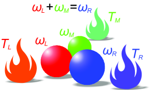
Figure 1: (Colour online) Three coupling qubits with the transition frequencies $\omega_{L}$, $\omega_{M}$, and $\omega_{R}$ are in contact with three separate baths at temperatures $T_{L}$, $T_{M}$, and $T_{R}$, where $\omega_{L}+\omega_{M}=\omega_{R}$ means the resonant coupling.

Let us consider that three coupling qubits interact with three heat baths, as is sketched in Fig. 1. The transition frequencies of the three qubits are denoted by $\omega_{L}$, $\omega_{M}$ and $\omega_{R}$, and the temperatures of the three baths are represented by $T_{L}$, $T_{M}$, and $T_{R}$, where the subscripts correspond to the qubits they are in contact with. Here we suppose that three qubits resonantly interact with each other, that is, $\omega_{L}+\omega_{M}=\omega_{R}$ is implied and without loss of generality, we let $\omega_{R}>\omega_{L}>\omega_{M}$. In such a model, the only resources driving the model to work are the three heat baths. One will see that such a model will act as a multifunctional quantum thermal device as considered throughout the paper. To show this, we will have to begin with the dynamics of the open system.

The Hamiltonian of the three interacting qubits reads

$$H_{S}=H_{0}+H_{I},$$ (1)

where the free Hamiltonian is

$$H_{0}=\sum_{\mu=L,M,R}\frac{1}{2}\omega_{\mu}\sigma_{\mu}^{z},$$ (2)

and the resonant internal interaction Hamiltonian is

$$H_{I}=g\sigma_{L}^{x}\sigma_{M}^{x}\sigma_{R}^{x},$$ (3)

with $\sigma^{x}$ and $\sigma^{z}$ denoting the Pauli matrices, $g$ denoting the coupling strength. Hereinafter we set the Planck constant and the Boltzmann constant to be unit, i.e., $\hbar=k_{B}=1$ for simplicity. Note that this type interaction Hamiltonian has been proposed and studied in some spin systems Reiss et al. (2003); Pachos and Plenio (2004); Bermudez et al. (2009); Seah et al. (2018). Furthermore let the three qubits contact with three heat baths with the Gibbs state $\rho_{\mu}=\exp{(-H_{\mu}/T_{\mu})}/{\mathrm{Tr}[\exp{(-H_{\mu}/T_{\mu})}]}$ where $H_{\mu}=\sum_{k}\omega_{\mu k}b^{\dagger}_{\mu k}b_{\mu k}$, $\mu=L,M,R$ respectively, $\omega_{\mu k}$ and $b_{\mu k}$ denote the frequencies and the annihilation operators of the bath mode with $[b_{\mu k},b_{\nu k^{{}^{\prime}}}^{\dagger}]=\delta_{\mu,\nu}\delta_{k,k^{{}^{\prime}}},[b_{\mu k}^{\dagger},b_{\nu k^{{}^{\prime}}}^{\dagger}]=0,[b_{\mu k},b_{\nu k^{{}^{\prime}}}]=0$. The interaction Hamiltonian between the system and the baths is given by

$$H_{SB}=\sum_{\mu k}f_{\mu k}\sigma_{\mu}^{x}(b_{\mu k}+b_{\mu k}^{\dagger}),$$ (4)

where $f_{\mu k}$ stands for the coupling strength between the $\mu$th qubit and the $k$th mode in its bath. Thus the total Hamiltonian of the whole system including the baths and the qubits can be written as

$$H_{total}=H_{S}+\sum_{\mu}H_{\mu}+H_{SB}.$$ (5)

To derive the master equation that governs the evolution of our open system, we have to turn to the $H_{S}$ representation. To do so, let’s consider the eigen-decomposition of $H_{S}$ as

$$H_{S}=\sum_{k}\lambda_{k}\left|\lambda_{k}\right\rangle\left\langle\lambda_{k}\right|$$ (6)

where the eigenvalues read

$$-\lambda_{1+j}=\lambda_{8-j}=\sqrt{\Lambda_{1+j}^{2}+g^{2}},j=0,1,2,3,$$ (7)

with $[\mathit{\Lambda}_{1},\mathit{\Lambda}_{2},\mathit{\Lambda}_{3},\mathit{\Lambda}_{4}]=[\omega_{R},\omega_{L},\omega_{M},0]$, and the eigenvectors are explicitly given in the Appendix. Thus the interaction Hamiltonian $H_{SB}$ in $H_{S}$ representation can be rewritten as

$$H_{SB}=\sum_{\mu,k,l}f_{\mu k}(V_{\mu l}(\omega_{\mu l})+V_{\mu l}^{\dagger}(\omega_{\mu l}))(b_{\mu k}+b_{\mu k}^{\dagger}),$$

where the eigenoperator $V_{\mu l}(\omega_{\mu l})$ of $H_{S}$ and their corresponding to the eigenfrequencies $\omega_{\mu l}$ satisfy the relation $[H_{S},V_{\mu l}(\omega_{\mu l})]=-\omega_{\mu l}V_{\mu l}(\omega_{\mu l})$ and their explicit expressions are also given in the Appendix. Therefore, following the standard procedure Breuer and Petruccione (2002), one can apply the Born-Markovian approximation and the secular approximation to obtain the master equation Breuer and Petruccione (2002) as

$$\dot{\rho}=-\mathrm{i}[H_{S},\rho]+\mathcal{L}_{L}[\rho]+\mathcal{L}_{M}[\rho]+\mathcal{L}_{R}[\rho],$$ (8)

where $\rho$ is the density matrix of the system and the Lindblad operator $\mathcal{L}_{\mu}[\rho]$ is given by

$$\mathcal{L}_{\mu}[\rho] =\sum_{l}J_{\mu}(-\omega_{\mu l})[2V_{\mu l}(\omega_{\mu l})\rho V_{\mu l}^{\dagger}(\omega_{\mu l})$$

$$-\{V_{\mu l}^{\dagger}(\omega_{\mu l})V_{\mu l}(\omega_{\mu l}),\rho\}]$$

$$+J_{\mu}(+\omega_{\mu l})[2V_{\mu l}^{\dagger}(\omega_{\mu l})\rho V_{\mu l}(\omega_{\mu l})$$

$$-\{V_{\mu l}(\omega_{\mu l})V_{\mu l}^{\dagger}(\omega_{\mu l}),\rho\}],$$ (9)

with the spectral densities defined by

$$J_{\mu}(\pm\omega_{\mu l})=\pm\gamma_{\mu}(\omega_{\mu l})n(\pm\omega_{\mu l}),$$ (10)

and the average thermal excitation number defined by

$$n(\omega_{\mu l})=\frac{1}{\mathrm{e}^{\frac{\omega_{\mu l}}{T_{\mu}}}-1}$$ (11)

subject to the frequency $\omega_{\mu l}$ and the temperature $T_{\mu}$. During the derivation of the master equation, the secular approximation requires the relaxation time of the system $\tau_{R}\sim 1/\gamma_{\mu}(\omega_{\mu l})$ is large compared to the typical time scale of the intrinsic evolution of the system $\tau_{S}\sim{|\omega_{\mu l}-\omega_{\mu l^{\prime}}|}^{-1}$. So we have the condition $\gamma_{\mu}(\omega_{\mu l})\ll\{|\omega_{\mu l}-\omega_{\mu l^{\prime}}|\}$ which signifies that the strong internal coupling strength greatly separates the energy levels. This is consistent with the conclusion in references Hofer et al. (2017b); González et al. (2017); Rivas et al. (2010); Seah et al. (2018) where the valid internal coupling strength regime is discussed via different master equations, such as local, global and coarse-graining master equations. Most importantly, the global master equation in the strong internal coupling strength regime coincides well with the laws of thermodynamics as shown in the above references. Definitely different bath spectra lead to different physical phenomenons Breuer and Petruccione (2002); Valleau et al. (2012). In the following text we assume $\gamma_{\mu}(\omega_{\mu l})=\gamma_{\mu}$ does not depend on the transition frequency for simplicity. Note that we also have tested the Ohmic bath spectrum and found that similar quantum thermal functions can be achieved given appropriate parameters. Only the difference between the valves using the two different bath spectra is present in Fig. 4.

The dynamical behavior of the system at any time is determined by the master equation Eq. (8). However, we concern its behaviour at the steady state in order to construct thermal device about heat current. Therefore what to do first is to solve the steady state solution of Eq. (8), i.e. $\dot{\rho}_{S}=0$. After some arrangement of steady state solution, one can obtain a system of linear equations about the elements of the density matrix as

$$\sum_{\mu=M,L,R}\mathbf{M}_{\mu}\left|\rho\right\rangle=0,\quad\rho_{ij}^{S}=0,i\neq j,$$ (12)

where $\left|\rho\right\rangle^{T}=[\rho_{11}^{S},\rho_{22}^{S},...,\rho_{88}^{S}]$ with

$$\mathbf{M}_{L} =(C_{1,1;3,2}+C_{6,1;8,2})\mathbf{J}_{L1}(C_{1,1;3,2}^{\dagger}+C_{6,1;8,2}^{\dagger})$$

$$+(C_{1,1;6,2}+C_{3,1;8,2})\mathbf{J}_{L2}(C_{1,1;6,2}^{\dagger}+C_{3,1;8,2}^{\dagger})$$

$$+(C_{2,1;4,2}+C_{5,1;7,2})\mathbf{J}_{L3}(C_{2,1;4,2}^{\dagger}+C_{5,1;7,2}^{\dagger})$$

$$+(C_{2,1;5,2}+C_{4,1;7,2})\mathbf{J}_{L4}(C_{2,1;5,2}^{\dagger}+C_{4,1;7,2}^{\dagger}),$$ (13)

$$\mathbf{M}_{M} =(C_{1,1;2,2}+C_{7,1;8,2})\mathbf{J}_{M1}(C_{1,1;2,2}^{\dagger}+C_{7,1;8,2}^{\dagger})$$

$$+(C_{1,1;7,2}+C_{2,1;8,2})\mathbf{J}_{M2}(C_{1,1;7,2}^{\dagger}+C_{2,1;8,2}^{\dagger})$$

$$+(C_{3,1;4,2}+C_{5,1;6,2})\mathbf{J}_{M3}(C_{3,1;4,2}^{\dagger}+C_{5,1;6,2}^{\dagger})$$

$$+(C_{3,1;5,2}+C_{4,1;6,2})\mathbf{J}_{M4}(C_{3,1;5,2}^{\dagger}+C_{4,1;6,2}^{\dagger}),$$ (14)

$$\mathbf{M}_{R} =(C_{1,1;4,2}+C_{5,1;8,2})\mathbf{J}_{R1}(C_{1,1;4,2}^{\dagger}+C_{5,1;8,2}^{\dagger})$$

$$+(C_{1,1;5,2}+C_{4,1;8,2})\mathbf{J}_{R2}(C_{1,1;5,2}^{\dagger}+C_{4,1;8,2}^{\dagger})$$

$$+(C_{2,1;3,2}+C_{6,1;7,2})\mathbf{J}_{R3}(C_{2,1;3,2}^{\dagger}+C_{6,1;7,2}^{\dagger})$$

$$+(C_{2,1;6,2}+C_{3,1;7,2})\mathbf{J}_{R4}(C_{2,1;6,2}^{\dagger}+C_{3,1;7,2}^{\dagger}).$$ (15)

Here $\mathbf{J}_{\mu l}=\begin{pmatrix}1&0\\ 0&0\end{pmatrix}\otimes\begin{pmatrix}1&0\\ 0&0\end{pmatrix}\otimes\begin{pmatrix}-B_{\mu l}&A_{\mu l}\\ B_{\mu l}&-A_{\mu l}\end{pmatrix}$ with $A_{\mu l}=\exp(\omega_{\mu l}/T_{\mu})B_{\mu l}$, $B_{\mu l}=\gamma_{\mu}n(\omega_{\mu l}){\sin}^{2}{\alpha_{\mu l}}$, and $C_{i,j;m,n}=\left|i\right\rangle\left\langle j\right|+\left|m\right\rangle\left\langle n\right|$ with $\left\{\left|i\right\rangle\right\}$ representing the natural orthonormal basis of $8$-dimensional Hilbert space. The negative sign in $\mathbf{J}_{\mu l}$ denotes the population decrement from a relevant level while the positive sign means the population increment. Based on the steady state solution, one can obtain the heat currents as Levy et al. (2012); Szczygielski et al. (2013); Kolář et al. (2012)

$$\dot{Q}_{\mu}=\mathrm{Tr}(H_{S}\mathcal{L}_{\mu}[\rho^{S}])=\left\langle\lambda\right|\mathbf{M}_{\mu}\left|\rho\right\rangle,$$ (16)

originating from the dissipation of the $\mu$th bath, where ${\left|\lambda\right\rangle}^{T}=[\lambda_{1},\lambda_{2},\lambda_{3},...,\lambda_{8}]$. One should note that $\dot{Q}_{\mu}>0$ denotes the system absorbing heat from the $\mu$th bath, while $\dot{Q}_{\mu}<0$ means that the heat flows into the bath. So the remaining key task is to solve the steady state solution of the master equation Eq. (12). However, the analytical solution of Eq. (12) is so tedious that we cannot explicitly give it here, so we would like to demonstrate the various thermodynamic functions based on the numerical solution in the next section.

III The various thermodynamic functions

The essence of a quantum thermal device is that the heat currents can be purposively controlled. In this section, we will show that our system can work as a thermal device with multiple different thermodynamic functions such as amplifier, modulator, switcher, valve, stabilizer, and rectifier.

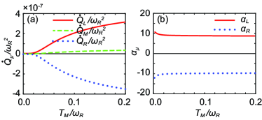
Figure 2: (Colour online) (a) Three heat currents $\dot{Q}_{\mu}/\omega_{R}^{2}$ versus $T_{M}/\omega_{R}$ at the steady state. The red solid, green dashed, and blue dotted lines correspond to the heat currents $\dot{Q}_{L}/\omega_{R}^{2}$, $\dot{Q}_{M}/\omega_{R}^{2}$, and $\dot{Q}_{R}/\omega_{R}^{2}$, respectively. (b) The amplification factors $\alpha_{\mu}$ versus $T_{M}/\omega_{R}$ at the steady state. The red solid and blue dotted lines correspond to $\alpha_{L}$ and $\alpha_{R}$, respectively. Here $\omega_{L}=0.9\omega_{R}$, $\omega_{M}=0.1\omega_{R}$, $g=0.1\omega_{M}$, $\gamma_{L}=\gamma_{M}=\gamma_{R}=\gamma=10^{-4}\omega_{R}$, $T_{L}=0.2\omega_{R}$, and $T_{R}=0.02\omega_{R}$.

Amplifier–The thermal amplifier means that a weak heat current at one terminal can significantly amplify the heat currents through the other two terminals ones. The ability of the amplifier is quantified by the amplification factor, for instance Joulain et al. (2016),

$$\alpha_{L,R}=\frac{\partial\dot{Q}_{L,R}}{\partial\dot{Q}_{M}},$$ (17)

where the heat current $\dot{Q}_{M}$ as the weak current to control the other two heat currents is implied. Strictly speaking, an amplifier is achieved if the amplification factor $\alpha_{L,R}>1$. The larger the amplification factor is, the better the amplification function is. We show the heat currents and the amplification factors in Fig. 2 (a) varying with $T_{M}$ for the internal coupling strength $g=0.1\omega_{M}$ in the case of the steady state. It is obvious that $\dot{Q}_{M}$ is small in the reasonable range of the temperature $T_{M}$, while the other two currents $\dot{Q}_{L}$ and $\dot{Q}_{R}$ are drastically changed. Fig. 2 (b) shows that the amplification factor versus the temperature $T_{M}$. It can be easily found that the absolute amplification factors $\left|\alpha_{L,R}\right|$ are about $10$ which shows that our system has the very strong amplification ability.

Modulator–A thermal modulator is used to modulate the heat currents continuously such that they can be changed from a small value to a large one by controlling a weak heat current. One can see from Fig. 2 that with the slight change of the heat current $\dot{Q}_{M}$, the heat currents $\dot{Q}_{L,R}$ have been modulated from almost zero value at a low temperature $T_{M}$ to a large value at a high temperature $T_{M}$. In fact, such a phenomenon can also be found in Fig. 3 where the heat currents $\dot{Q}_{L,R}$ vary from a tiny value to a large value. These are just the modulation function.

Switcher– The heat switcher can “cut off” the heat currents if one weak heat current becomes weak enough. This function is quite obvious from Fig. 2 (a) and Fig. 3. In Fig. 2 (a), one can see that the currents will almost vanish when the temperature $T_{M}$ at the “control” terminal become small. Similarly, in Fig. 3, the heat currents will reach zero when the temperature $T_{L/R}$ as the “control” terminal approaches a given value.

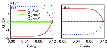
Figure 3: (Colour online) Three heat currents $\dot{Q}_{\mu}/\omega_{R}^{2}$ (a) versus $T_{L}/\omega_{R}$ and (b) versus $T_{R}/\omega_{R}$ at the steady state. The red solid, green dashed, and blue dotted lines correspond to the heat currents $\dot{Q}_{L}/\omega_{R}^{2}$, $\dot{Q}_{M}/\omega_{R}^{2}$, and $\dot{Q}_{R}/\omega_{R}^{2}$, respectively. Here $\omega_{L}=0.9\omega_{R}$, $\omega_{M}=0.1\omega_{R}$, $g=0.8\omega_{M}$, $\gamma_{L}=\gamma_{M}=\gamma_{R}=\gamma=10^{-4}\omega_{R}$. In addition, in (a) $T_{R}=0.12\omega_{R}$, $T_{M}=0.08\omega_{R}$, and in (b) $T_{L}=0.12\omega_{R}$, $T_{M}=0.08\omega_{R}$.

Stabilizer–The feature of a heat stabilizer is that the heat currents are robust to the fluctuation of the temperature. Here we will show that our model can work as a stabilizer because the currents are not sensitive to the change of the temperature $T_{L}$ or $T_{R}$. As displayed in Fig. 3 (a), the three currents are obviously not sensitive to the change of the temperature $T_{L}$ over the large range from $T_{L}=0$ to around $T_{L}=0.8\omega_{R}$. The reason is that the greatly separated transition frequency $\omega_{L}=0.9\omega_{R}$ is much larger than $T_{L}$ which prevents the bath $L$ to drastically excite the qubit $L$’s transition, which can be verified from Eqs. (10)-(11). This situation is also suitable for $T_{R}$ as presented in Fig. 3 (b). Although the coupling strength is set as $g=0.8\omega_{M}$, one can check that $stabilizer$ function still exists for relatively weak coupling $g$ which shows that the contribution of the interaction has the limited influence on the stabilizer compared with the difference of the transition frequencies.

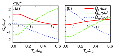
Figure 4: (Colour online) Three heat currents $\dot{Q}_{\mu}/\omega_{R}^{2}$ versus $T_{M}/\omega_{R}$ at the steady state. The red solid, green dashed, and blue dotted lines correspond to currents $\dot{Q}_{L}/\omega_{R}^{2}$, $\dot{Q}_{M}/\omega_{R}^{2}$, and $\dot{Q}_{R}/\omega_{R}^{2}$, respectively. Here we have $\omega_{L}=0.6\omega_{R}$, $\omega_{M}=0.4\omega_{R}$, $g=0.8\omega_{M}$ fixed. In (a) the spontaneous decay rate $\gamma_{\mu}(\omega_{\mu l})=\gamma_{\mu}$ is chosen to be independent of frequency as mentioned before, i.e., $\gamma_{L}=\gamma_{M}=\gamma_{R}=\gamma=10^{-4}\omega_{R}$, and $T_{L}=0.25\omega_{R}$, $T_{R}=0.2\omega_{R}$, while in (b) the Ohmic spectrum is applied Carmichael (2002), i.e., $\gamma_{\mu}(\omega_{\mu l})=\gamma_{\mu}\omega_{\mu l}$, and $\gamma_{\mu}$ is constant as above. The temperatures are set as $T_{L}=0.45\omega_{R}$, $T_{R}=0.4\omega_{R}$. Obviously the valve function is also obtained at different critical temperature points.

Valve–In analogy to a classical valve, a quantum thermal valve can perfectly cut off the heat current at any one terminal and allow the heat to flow through the other two terminals. Here we consider the heat current $\dot{Q}_{M}$ as the control terminal. In order to see the valve function, we plot the three heat currents with respect to the temperature $T_{M}$ in Fig. 4. As we see in subfigure (a) where the spontaneous decay rate is set independent of frequency, when the temperature $T_{M}$ approaches to a critical temperature (about $0.09$), the heat current $\dot{Q}_{R}$ is cut off and the heat can freely flow through the other two terminals. When $T_{M}$ reaches another critical temperature (about $0.24$), the heat current $\dot{Q}_{M}$ is cut off. When the $T_{M}$ reaches the third critical temperature (about $0.53$), the heat current $\dot{Q}_{L}$ is cut off. In fact, the direction of the currents can also be easily switched by controlling one temperature $T_{M}$. If the Ohmic spectrum of the bath is chosen, similar valve function can also be achieved as shown in subfigure (b) with different appropriate temperatures.

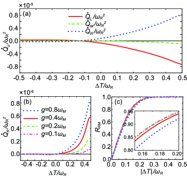
Figure 5: (Colour online) (a) Three heat currents $\dot{Q}_{\mu}/\omega_{R}^{2}$ versus $\Delta T/\omega_{R}=(T_{R}-T_{M})/\omega_{R}$ with $g=0.8\omega_{M}$ and $T_{L}=0.18\omega_{R}$. (b) Heat current $\dot{Q}_{R}/\omega_{R}^{2}$ versus $\Delta T/\omega_{R}=(T_{R}-T_{M})/\omega_{R}$ for different coupling strength $g$ without the bath $L$. (c) The rectification factors $R_{RM}$ versus $|\Delta T|/\omega_{R}=|(T_{R}-T_{M})|/\omega_{R}$ corresponding to the cases in (b), and the inset is a close-up image over the range of $0.15<|\Delta T|/\omega_{R}<0.2$. In all the cases the spontaneous decay rates $\gamma_{L}=\gamma_{M}=\gamma_{R}=\gamma=10^{-4}\omega_{R}$, $\omega_{L}=0.9\omega_{R}$, $\omega_{M}=0.1\omega_{R}$, and the average temperature $T_{A}=(T_{R}+T_{M})/2=0.25\omega_{R}$ are fixed. The blue dotted, red solid, green dashed, and magenta dot-dash lines correspond to $g=0.8\omega_{M}$, $g=0.4\omega_{M}$, $g=0.2\omega_{M}$, and $g=0.1\omega_{M}$ in (b) and (c), respectively.

Rectifier–The significant feature of a rectifier is to allow the thermal current flow unidirectionally, which is an analogue of the classical rectifier of the electricity. In Fig. 5 (a), we plot the heat currents at the terminals $R$ and $M$ versus the temperature difference $\Delta T=T_{R}-T_{M}$. It is obvious that when $\Delta T$ is larger than a critical value ($\sim-0.1$), the heat flows along a certain direction, for example, the heat flows out of the bath $R$ and into the bath $M$ (as well as bath $L$). Here we’d better consider the terminal $M$ and $L$ as a whole to serve as the common terminal. On the contrary, if $\Delta T$ is less than the critical value, the almost vanishing heat will flow oppositely. So our system can work as a rectifier. However, one can find that the critical value does not lie at the zero temperature difference, which means that swapping the heat baths $R$ and $M$ cannot change the direction of heat current with a small temperature difference. This is actually due to the existence of the third heat current $\dot{Q}_{L}$. To avoid this effect, we remove the bath $L$ so that the critical temperature difference can be translated to zero value. Meanwhile, our system can become a two-terminal quantum thermal device Maznev et al. (2013); Ordonez-Miranda et al. (2017). In this case, the rectification factor, quantifying the ability of rectification, can be well defined as Marcos-Vicioso et al. (2018)

$$R=\frac{|\dot{Q}_{fore}-\dot{Q}_{back}|}{|\dot{Q}_{fore}+\dot{Q}_{back}|}.$$ (18)

The larger $R$ signifies the better rectification ability, and a perfect rectifier is obtained for $R=1$. In Fig. 5 (b) we plot the heat current $\dot{Q}_{R}$ with respect to the temperature difference $\Delta T$ for different $g$ and different $\omega_{L}$. It is obvious that the considerable heat current can only flow along a single direction, and the strong internal coupling is more beneficial to the large unidirectional heat current. In Fig. 5 (c), the rectification factors $R_{RM}$ corresponding to Fig. 5 (b) versus the absolute temperature difference $|\Delta T|$ are plotted. Note that we have let $\dot{Q}_{fore}=\dot{Q}_{R}$ for $T_{R}>T_{M}$ while $\dot{Q}_{back}=-\dot{Q}_{R}$ for $T_{R}<T_{M}$. We can also notice that large temperature difference results in almost perfect rectification. Similarly the rectification effect can also be found if the bath $R$ is removed.

IV Discussion

Before the end, we would like to give an intuitive but rough understanding to our device. A helpful way is to image our device has only three eigenfrequencies (levels) which satisfy the resonance condition, but two of which are extremely different. It is natural that two eigenfrequencies are relatively close to each other. Suppose each transition is driven by a thermal bath. Such a configuration is much like the quantum refrigerator presented in Ref. Linden et al. (2010). Due to the energy conservation, the output heat current released only by the transition subject to the maximal eigenfrequencies must be the same as the total input heat currents shared by the other two transitions subject to quite different eigenfrequencies. Since the two relatively close eigenfrequencies are separated in the input and the output terminals respectively, they should govern the similar large magnitude of the change of the heat currents. Correspondingly, the heat current at the third terminal will be only slightly changed. In the different parameter regimes, the input and output heat currents will be shared by different combinations of the three eigenfrequencies. So various interesting functions will appear. Compared with our current device with eight eigenfrequencies, it includes many similar three-level transitions as above. However, they don’t work separately (which directly leads to the difficulty to directly understand our device physically). Their cooperative effect can lead to much more complicated transitions and hence could enhance or reduce the working mechanism mentioned for the three-level case. In one word, the plentiful functions result from the asymmetry and the complexity (the strong internal coupling) of the covered transitions in the system, while one specific function made to be superior to the others results from the proper choice of the parameter regimes.

Furthermore, one has to note that designing our quantum thermal device is greatly related to the choice of the system’s structure and dissipation channels including the temperatures of the baths. As we know, both the transistor and the rectifier need the asymmetry of transition frequencies at the different terminals, the stabilizer requires the working transition frequencies are much larger than their corresponding temperature in terms of numerical value, and the valve only needs that the heat currents can selectively vanish. Whether these functions above can be realized in some simpler systems such as a single qubit, qutrit or two qubits system remains an interesting question. However, one can easily check that, given the same spontaneous decay rates, the rectifier and the transistor are hard to implement in qubit systems Segal and Nitzan (2005) due to lack of the asymmetric level configuration. The valve cannot be implemented in a qutrit due to the heat currents generally vanish simultaneously. In addition, the multi-level system of a single qudit (e.g. a qutrit) usually leads to the cross couplings between a single transition with different baths. For the two-qubit system such as Ref. Man et al. (2016), the transistor function is not found (Here we do not use the rotating wave approximation), the reason is that two baths have to share the same dissipation channels via a single qubit, otherwise, the cross coupling could also be covered.

In addition, we want to emphasize that the choice of the three qubits’ transition frequencies is related to the validity of global master equation and the system’s thermal function. On one hand, the secular approximation has to be satisfied in the derivation of global master equation as shown in Seah et al. (2018); González et al. (2017); Hofer et al. (2017b); Breuer and Petruccione (2002). It means the energy gap should be much greater compared with the system’s decay rates. Any two qubits in our model possessing the same transition frequencies will generate the degenerate levels which result in the violation of the secular approximation no matter how strong the internal coupling is. On the other hand, there are only three energy configurations, i.e., $\omega_{R}$ equal to, larger or smaller than $\omega_{L}+\omega_{M}$ given three baths can be at any temperature. Similar functions can also be realized in these cases. What we should pay attention to is cautiously arranging their energy distribution especially for the transistor and rectifier that need greatly asymmetric energy levels as well known.

Finally, we will give a brief discussion about the possible experimental realization. As well known, a spin-like system can be easily realized, the key is how to realize trilinear interaction in a system. In Refs. Reiss et al. (2003); Pachos and Plenio (2004); Bermudez et al. (2009), the authors have proposed how to construct a system with internal trilinear interaction. Especially in Bermudez et al. (2009), Bermudez et al. employed many spin-like trapped ions to construct a Hamiltonian including bilinear and trilinear coupling by modifying external fields. The transition frequency of each ion and both the coupling strengths can be carefully adjusted. Zero strength of the bilinear coupling leads to our model. The coupling between the system and a bath can be achieved via a resonator, and a resistor act as a bathKarimi et al. (2017); Cottet et al. (2017). In fact, the reservoir could be directly tailored with the desired bath spectrum by reservoir engineering, which has been described in detail and applied in many casesScovil and Schulz-DuBois (1959); Gelbwaser-Klimovsky et al. (2013); Myatt et al. (2000); Gröblacher et al. (2015). Note that as our model is general and the valid temperature regime is related to the choice of a qubit’s frequency, so one can modify the desired temperature according to the qubit’s frequency.

V Conclusion

In this paper, a multifunctional quantum thermal device has been designed by utilizing three resonantly and strongly internal coupling qubits in contact with three heat baths. We study transport properties by applying the secular master equation. The steady-state thermal behaviours show that this thermal device can work as a thermal transistor, a switcher, a valve and even a thermal rectifier. We would like to emphasize that the plenty of the functions mainly originate from the large difference between the transition frequencies of the qubits. Whether it could induce some more novel applications is worthy of being studied in the future.

Appendix A The eigen-decomposition of $H_{S}$ and the eigen-operators

For the Hamiltonian $H_{S}$, the eigen-decomposition reads $H_{S}=\sum_{k}\lambda_{k}\left|\lambda_{k}\right\rangle\left\langle\lambda_{k}\right|$, where the eigenvalues $\lambda_{k}$ are given in the main text and the eigenvectors are given as follows.

$$\left|\lambda_{1}\right\rangle =-\sin\theta_{1}\left|111\right\rangle+\cos\theta_{1}\left|000\right\rangle,$$

$$\left|\lambda_{2}\right\rangle =-\sin\theta_{2}\left|101\right\rangle+\cos\theta_{2}\left|010\right\rangle,$$

$$\left|\lambda_{3}\right\rangle =-\cos\theta_{3}\left|100\right\rangle+\sin\theta_{3}\left|011\right\rangle,$$

$$\left|\lambda_{4}\right\rangle =-\cos\theta_{4}\left|110\right\rangle+\sin\theta_{4}\left|001\right\rangle,$$

$$\left|\lambda_{5}\right\rangle =+\sin\theta_{4}\left|110\right\rangle+\cos\theta_{4}\left|001\right\rangle,$$ (19)

$$\left|\lambda_{6}\right\rangle =+\sin\theta_{3}\left|100\right\rangle+\cos\theta_{3}\left|011\right\rangle,$$

$$\left|\lambda_{7}\right\rangle =+\cos\theta_{2}\left|101\right\rangle+\sin\theta_{2}\left|010\right\rangle,$$

$$\left|\lambda_{8}\right\rangle =+\cos\theta_{1}\left|111\right\rangle+\sin\theta_{1}\left|000\right\rangle,$$

with $\sin\theta_{i}=g/\sqrt{[\sqrt{(\mathit{\Lambda}_{i}^{2}+g^{2})}+\mathit{\Lambda}_{i}]^{2}+g^{2}}$, $\cos\theta_{i}=\sqrt{1-{\sin}^{2}\theta_{i}}$, ${\left|1\right\rangle}_{\mu}={[1,0]}^{T}$ and ${\left|0\right\rangle}_{\mu}={[0,1]}^{T}$ representing the excited and the ground states of the $\mu$th qubit. Thus the transition operators of the qubits can also be rewritten in the $H_{S}$ representation as

$$V_{L1} =\sin\alpha_{L1}(\left|\lambda_{6}\right\rangle\left\langle\lambda_{8}\right|-\left|\lambda_{1}\right\rangle\left\langle\lambda_{3}\right|),$$

$$V_{L2} =\sin\alpha_{L2}(\left|\lambda_{1}\right\rangle\left\langle\lambda_{6}\right|+\left|\lambda_{3}\right\rangle\left\langle\lambda_{8}\right|),$$

$$V_{L3} =\sin\alpha_{L3}(\left|\lambda_{5}\right\rangle\left\langle\lambda_{7}\right|-\left|\lambda_{2}\right\rangle\left\langle\lambda_{4}\right|),$$

$$V_{L4} =\sin\alpha_{L4}(\left|\lambda_{2}\right\rangle\left\langle\lambda_{5}\right|+\left|\lambda_{4}\right\rangle\left\langle\lambda_{7}\right|),$$

$$V_{M1} =\sin\alpha_{M1}(\left|\lambda_{1}\right\rangle\left\langle\lambda_{2}\right|+\left|\lambda_{7}\right\rangle\left\langle\lambda_{8}\right|),$$

$$V_{M2} =\sin\alpha_{M2}(\left|\lambda_{2}\right\rangle\left\langle\lambda_{8}\right|-\left|\lambda_{1}\right\rangle\left\langle\lambda_{7}\right|),$$ (20)

$$V_{M3} =\sin\alpha_{M3}(\left|\lambda_{3}\right\rangle\left\langle\lambda_{4}\right|+\left|\lambda_{5}\right\rangle\left\langle\lambda_{6}\right|),$$

$$V_{M4} =\sin\alpha_{M4}(\left|\lambda_{3}\right\rangle\left\langle\lambda_{5}\right|-\left|\lambda_{4}\right\rangle\left\langle\lambda_{6}\right|),$$

$$V_{R1} =\sin\alpha_{R1}(\left|\lambda_{5}\right\rangle\left\langle\lambda_{8}\right|+\left|\lambda_{1}\right\rangle\left\langle\lambda_{4}\right|),$$

$$V_{R2} =\sin\alpha_{R2}(\left|\lambda_{1}\right\rangle\left\langle\lambda_{5}\right|-\left|\lambda_{4}\right\rangle\left\langle\lambda_{8}\right|),$$

$$V_{R3} =\sin\alpha_{R3}(\left|\lambda_{6}\right\rangle\left\langle\lambda_{7}\right|+\left|\lambda_{2}\right\rangle\left\langle\lambda_{3}\right|),$$

$$V_{R4} =\sin\alpha_{R4}(\left|\lambda_{2}\right\rangle\left\langle\lambda_{6}\right|-\left|\lambda_{3}\right\rangle\left\langle\lambda_{7}\right|),$$

where

$$\alpha_{Lk} =\frac{\mathrm{\pi}}{4}-\left(-1\right)^{k}\left(\frac{\mathrm{\pi}}{4}-(\theta_{[k]}-\theta_{[k]+2})\right),$$

$$\alpha_{Mk} =\frac{\mathrm{\pi}}{4}-\left(-1\right)^{k}\left(\frac{\mathrm{\pi}}{4}-(\theta_{[k]}-\theta_{[k]+1})\right),$$ (21)

$$\alpha_{Rk} =\frac{\mathrm{\pi}}{4}+\left(-1\right)^{k}\left(\frac{\mathrm{\pi}}{4}-(\theta_{[k]}+\theta_{5-[k]})\right),$$

with $[k]$ denoting the minimal integer not less than $k/2$, and the corresponding eigenfrequencies are given by

$$\omega_{L1,2} =\sqrt{\mathit{\Lambda}_{1}^{2}+g^{2}}\mp\sqrt{\mathit{\Lambda}_{3}^{2}+g^{2}},$$

$$\omega_{L3,4} =\sqrt{\mathit{\Lambda}_{2}^{2}+g^{2}}\mp\sqrt{\mathit{\Lambda}_{4}^{2}+g^{2}},$$

$$\omega_{M1,2} =\sqrt{\mathit{\Lambda}_{1}^{2}+g^{2}}\mp\sqrt{\mathit{\Lambda}_{2}^{2}+g^{2}},$$

$$\omega_{M3,4} =\sqrt{\mathit{\Lambda}_{3}^{2}+g^{2}}\mp\sqrt{\mathit{\Lambda}_{4}^{2}+g^{2}},$$ (22)

$$\omega_{R1,2} =\sqrt{\mathit{\Lambda}_{1}^{2}+g^{2}}\mp\sqrt{\mathit{\Lambda}_{4}^{2}+g^{2}},$$

$$\omega_{R3,4} =\sqrt{\mathit{\Lambda}_{2}^{2}+g^{2}}\mp\sqrt{\mathit{\Lambda}_{3}^{2}+g^{2}}.$$

It is obvious that the eigenoperators and their corresponding eigenfrequencies $\omega_{\mu l}$ satisfy $[H_{S},V_{\mu l}(\omega_{\mu l})]=-\omega_{\mu l}V_{\mu l}(\omega_{\mu l})$.

References

- Lashkaryov (1941) V. E. Lashkaryov, Investigations of a barrier layer by the thermoprobe method, Izv. Akad. Nauk SSSR, Ser. Fiz. 5, 422 (1941).
- Bardeen and Brattain (1998) J. Bardeen and W. H. Brattain, The transistor, a semiconductor triode, Proc. IEEE 86, 29 (1998).
- Levy et al. (2012) A. Levy, R. Alicki, and R. Kosloff, Quantum refrigerators and the third law of thermodynamics, Phys. Rev. E 85, 061126 (2012).
- Feldmann and Kosloff (2000) T. Feldmann and R. Kosloff, Performance of discrete heat engines and heat pumps in finite time, Phys. Rev. E 61, 4774 (2000).
- Palao et al. (2001) J. P. Palao, R. Kosloff, and J. M. Gordon, Quantum thermodynamic cooling cycle, Phys. Rev. E 64, 056130 (2001).
- Arnaud et al. (2002) J. Arnaud, L. Chusseau, and F. Philippe, Carnot cycle for an oscillator, Eur. J. Phys. 23, 489 (2002).
- Segal and Nitzan (2006) D. Segal and A. Nitzan, Molecular heat pump, Phys. Rev. E 73, 026109 (2006).
- de Tomás et al. (2012) C. de Tomás, A. C. Hernández, and J. M. M. Roco, Optimal low symmetric dissipation carnot engines and refrigerators, Phys. Rev. E 85, 010104 (2012).
- Geva and Kosloff (1992) E. Geva and R. Kosloff, A quantum-mechanical heat engine operating in finite time. a model consisting of spin- systems as the working fluid, J. Chem. Phys. 96, 3054 (1992).
- Geva and Kosloff (1996) E. Geva and R. Kosloff, The quantum heat engine and heat pump: An irreversible thermodynamic analysis of the three鈥恖evel amplifier, J. Chem. Phys. 104, 7681 (1996).
- Kosloff and Feldmann (2010) R. Kosloff and T. Feldmann, Optimal performance of reciprocating demagnetization quantum refrigerators, Phys. Rev. E 82, 011134 (2010).
- Thomas and Johal (2011) G. Thomas and R. S. Johal, Coupled quantum otto cycle, Phys. Rev. E 83, 031135 (2011).
- Feldmann et al. (1996) T. Feldmann, E. Geva, R. Kosloff, and P. Salamon, Heat engines in finite time governed by master equations, Am. J. Phys. 64, 485 (1996).
- Feldmann and Kosloff (2003) T. Feldmann and R. Kosloff, Quantum four-stroke heat engine: Thermodynamic observables in a model with intrinsic friction, Phys. Rev. E 68, 016101 (2003).
- Quan et al. (2007) H. T. Quan, Y. X. Liu, C. P. Sun, and F. Nori, Quantum thermodynamic cycles and quantum heat engines, Phys. Rev. E 76, 031105 (2007).
- Linden et al. (2010) N. Linden, S. Popescu, and P. Skrzypczyk, How small can thermal machines be? the smallest possible refrigerator, Phys. Rev. Lett. 105, 130401 (2010).
- He et al. (2017) Z. C. He, X. Y. Huang, and C. S. Yu, Enabling the self-contained refrigerator to work beyond its limits by filtering the reservoirs, Phys. Rev. E 96, 052126 (2017).
- Yu and Zhu (2014) C. S. Yu and Q. Y. Zhu, Re-examining the self-contained quantum refrigerator in the strong-coupling regime, Phys. Rev. E 90, 052142 (2014).
- Man and Xia (2017) Z.-X. Man and Y.-J. Xia, Smallest quantum thermal machine: The effect of strong coupling and distributed thermal tasks, Phys. Rev. E 96, 012122 (2017).
- Silva et al. (2015) R. Silva, P. Skrzypczyk, and N. Brunner, Small quantum absorption refrigerator with reversed couplings, Phys. Rev. E 92, 012136 (2015).
- Abah et al. (2012) O. Abah, J. Roßnagel, G. Jacob, S. Deffner, F. Schmidt-Kaler, K. Singer, and E. Lutz, Single-ion heat engine at maximum power, Phys. Rev. Lett. 109, 203006 (2012).
- Roßnagel et al. (2016) J. Roßnagel, S. T. Dawkins, K. N. Tolazzi, O. Abah, E. Lutz, F. Schmidt-Kaler, and K. Singer, A single-atom heat engine, Science 352, 325 (2016).
- Alicki (1979) R. Alicki, The quantum open system as a model of the heat engine, J. Phys. A 12, L103 (1979).
- Skrzypczyk et al. (2011) P. Skrzypczyk, N. Brunner, N. Linden, and S. Popescu, The smallest refrigerators can reach maximal efficiency, J. Phys. A 44, 492002 (2011).
- Qin et al. (2017) M. Qin, H.Z. Shen, X.L. Zhao, and X.X. Yi, Effects of system-bath coupling on a photosynthetic heat engine: A polaron master-equation approach, Physical Review A 96 (2017), 10.1103/PhysRevA.96.012125, cited By 3.
- Ito et al. (2016) K. Ito, K. Nishikawa, and H. Iizuka, Multilevel radiative thermal memory realized by the hysteretic metal-insulator transition of vanadium dioxide, Appl. Phys. Lett. 108, 053507 (2016).
- Yang et al. (2013) Y. Yang, S. Basu, and L. P. Wang, Radiation-based near-field thermal rectification with phase transition materials, Appl. Phys. Lett. 103, 163101 (2013).
- Ito et al. (2014) K. Ito, K. Nishikawa, H. Iizuka, and H. Toshiyoshi, Experimental investigation of radiative thermal rectifier using vanadium dioxide, Appl. Phys. Lett. 105, 253503 (2014).
- Ben-Abdallah and Biehs (2014) P. Ben-Abdallah and S. A. Biehs, Near-field thermal transistor, Phys. Rev. Lett. 112, 044301 (2014).
- Joulain et al. (2015) K. Joulain, Y. Ezzahri, J. Drevillon, and P. Ben-Abdallah, Modulation and amplification of radiative far field heat transfer: Towards a simple radiative thermal transistor, Appl. Phys. Lett. 106, 133505 (2015).
- Wehmeyer et al. (2017) G. Wehmeyer, T. Yabuki, C. Monachon, J. Q. Wu, and C. Dames, Thermal diodes, regulators, and switches: Physical mechanisms and potential applications, Appl. Phys. Rev. 4, 041304 (2017).
- Marcos-Vicioso et al. (2018) A. Marcos-Vicioso, C. López-Jurado, M. Ruiz-Garcia, and R. Sánchez, Thermal rectification with interacting electronic channels: Exploiting degeneracy, quantum superpositions, and interference, Phys. Rev. B 98, 035414 (2018).
- Maznev et al. (2013) A. A. Maznev, A. G. Every, and O. B. Wright, Reciprocity in reflection and transmission: What is a ‘phonon diode’? Wave Motion 50, 776 – 784 (2013).
- Werlang et al. (2014) T. Werlang, M. A. Marchiori, M. F. Cornelio, and D. Valente, Optimal rectification in the ultrastrong coupling regime, Phys. Rev. E 89, 062109 (2014).
- Chen and Wang (2015) T. Chen and X. B. Wang, Thermal rectification in the nonequilibrium quantum-dots-system, Physica E 72, 58 (2015).
- Li et al. (2004) B. W. Li, L. Wang, and G. Casati, Thermal diode: Rectification of heat flux, Phys. Rev. Lett. 93, 184301 (2004).
- Pereira (2011) E. Pereira, Sufficient conditions for thermal rectification in general graded materials, Phys. Rev. E 83, 031106 (2011).
- Wang et al. (2012) J. Wang, E. Pereira, and G. Casati, Thermal rectification in graded materials, Phys. Rev. E 86, 010101 (2012).
- Kobayashi et al. (2009) W. Kobayashi, Y. Teraoka, and I. Terasaki, An oxide thermal rectifier, Appl. Phys. Lett. 95, 171905 (2009).
- Fratini and Ghobadi (2016) F. Fratini and R. Ghobadi, Full quantum treatment of a light diode, Phys. Rev. A 93, 023818 (2016).
- Landi et al. (2014) G. T. Landi, E. Novais, M. J. de Oliveira, and D. Karevski, Flux rectification in the quantum chain, Phys. Rev. E 90, 042142 (2014).
- Man et al. (2016) Z. X. Man, N. B. An, and Y. J. Xia, Controlling heat flows among three reservoirs asymmetrically coupled to two two-level systems, Phys. Rev. E 94, 042135 (2016).
- Jiang et al. (2015) J. H. Jiang, M. Kulkarni, D. Segal, and Y. Imry, Phonon thermoelectric transistors and rectifiers, Phys. Rev. B 92, 045309 (2015).
- Guo et al. (2018) B.-Q. Guo, T. Liu, and C.-S. Yu, Quantum thermal transistor based on qubit-qutrit coupling, Phys. Rev. E 98, 022118 (2018).
- Joulain et al. (2016) K. Joulain, J. Drevillon, Y. Ezzahri, and J. Ordonez-Miranda, Quantum thermal transistor, Phys. Rev. Lett. 116, 200601 (2016).
- Lo et al. (2008) W. C. Lo, L. Wang, and B. W. Li, Thermal transistor: Heat flux switching and modulating, J. Phys. Soc. Jpn. 77, 054402 (2008).
- Li et al. (2006) B. W. Li, L. Wang, and G. Casati, Negative differential thermal resistance and thermal transistor, Appl. Phys. Lett. 88, 143501 (2006).
- Komatsu and Ito (2011) T. S. Komatsu and N. Ito, Thermal transistor utilizing gas-liquid transition, Phys. Rev. E 83, 012104 (2011).
- Segal and Nitzan (2005) D. Segal and A. Nitzan, Heat rectification in molecular junctions, The Journal of Chemical Physics 122, 194704 (2005).
- Zhong et al. (2012) W.-R. Zhong, D.-Q. Zheng, and B. Hu, Thermal control in graphene nanoribbons: thermal valve, thermal switch and thermal amplifier, Nanoscale 4, 5217–5220 (2012).
- Wang and Li (2007) L. Wang and B. W. Li, Thermal logic gates: Computation with phonons, Phys. Rev. Lett. 99, 177208 (2007).
- Wang and Li (2008) L. Wang and B. W. Li, Thermal memory: A storage of phononic information, Phys. Rev. Lett. 101, 267203 (2008).
- Faucheux et al. (1995) L. P. Faucheux, L. S. Bourdieu, P. D. Kaplan, and A. J. Libchaber, Optical thermal ratchet, Phys. Rev. Lett. 74, 1504 (1995).
- Zhan et al. (2009) F. Zhan, N. B. Li, S. Kohler, and P. Hänggi, Molecular wires acting as quantum heat ratchets, Phys. Rev. E 80, 061115 (2009).
- Hofer et al. (2017a) P. P. Hofer, J. B. Brask, M. Perarnau-Llobet, and N. Brunner, Quantum thermal machine as a thermometer, Phys. Rev. Lett. 119, 090603 (2017a).
- Binder et al. (2015) F. C. Binder, S. Vinjanampathy, K. Modi, and J. Goold, Quantacell: powerful charging of quantum batteries, New J. Phys. 17, 075015 (2015).
- Campaioli et al. (2017) F. Campaioli, F. A. Pollock, F. C. Binder, L. Céleri, J. Goold, S. Vinjanampathy, and K. Modi, Enhancing the charging power of quantum batteries, Phys. Rev. Lett. 118, 150601 (2017).
- Ferraro et al. (2018) D. Ferraro, M. Campisi, G. M. Andolina, V. Pellegrini, and M. Polini, High-power collective charging of a solid-state quantum battery, Phys. Rev. Lett. 120, 117702 (2018).
- Breuer and Petruccione (2002) H. P. Breuer and F. Petruccione, The Theory of Open Quantum Systems (Oxford University Press, Oxford, UK, 2002).
- Reiss et al. (2003) T. O. Reiss, N. Khaneja, and S. J. Glaser, Broadband geodesic pulses for three spin systems: time-optimal realization of effective trilinear coupling terms and indirect swap gates, J. Magn. Reson. 165, 95 (2003).
- Pachos and Plenio (2004) J. K. Pachos and M. B. Plenio, Three-spin interactions in optical lattices and criticality in cluster hamiltonians, Phys. Rev. Lett. 93, 056402 (2004).
- Bermudez et al. (2009) A. Bermudez, D. Porras, and M. A. Martin-Delgado, Competing many-body interactions in systems of trapped ions, Phys. Rev. A 79, 060303 (2009).
- Seah et al. (2018) S. Seah, S. Nimmrichter, and V. Scarani, Refrigeration beyond weak internal coupling, Phys. Rev. E 98, 012131 (2018).
- Hofer et al. (2017b) P. P. Hofer, M. Perarnau-Llobet, L. D. M. Miranda, G. Haack, R. Silva, J. B. Brask, and N. Brunner, Markovian master equations for quantum thermal machines: local versus global approach, New Journal of Physics 19, 123037 (2017b).
- González et al. (2017) J. O. González, L. A. Correa, G. Nocerino, J. P. Palao, D. Alonso, and G. Adesso, Testing the validity of the ‘local’ and ‘global’ gkls master equations on an exactly solvable model, Open Systems & Information Dynamics 24, 1740010 (2017).
- Rivas et al. (2010) Á. Rivas, A. D. K. Plato, S. F. Huelga, and M. B. Plenio, Markovian master equations: a critical study, New Journal of Physics 12, 113032 (2010).
- Valleau et al. (2012) S. Valleau, A. Eisfeld, and A. Aspuru-Guzik, On the alternatives for bath correlators and spectral densities from mixed quantum-classical simulations, The Journal of Chemical Physics 137, 224103 (2012).
- Szczygielski et al. (2013) K. Szczygielski, D. Gelbwaser-Klimovsky, and R. Alicki, Markovian master equation and thermodynamics of a two-level system in a strong laser field, Phys. Rev. E 87, 012120 (2013).
- Kolář et al. (2012) M. Kolář, D. Gelbwaser-Klimovsky, R. Alicki, and G. Kurizki, Quantum bath refrigeration towards absolute zero: Challenging the unattainability principle, Phys. Rev. Lett. 109, 090601 (2012).
- Carmichael (2002) H. J. Carmichael, Statistical Methods in Quantum Optics 1. Master Equations and Fokker–Planck Equations (2002).
- Ordonez-Miranda et al. (2017) J. Ordonez-Miranda, Y. Ezzahri, and K. Joulain, Quantum thermal diode based on two interacting spinlike systems under different excitations, Phys. Rev. E 95, 022128 (2017).
- Karimi et al. (2017) B. Karimi, J. P. Pekola, M. Campisi, and R. Fazio, Coupled qubits as a quantum heat switch, Quantum Science and Technology 2, 044007 (2017).
- Cottet et al. (2017) N. Cottet, S. Jezouin, L. Bretheau, P. Campagne-Ibarcq, Q. Ficheux, J. Anders, A. Auffèves, R. Azouit, P. Rouchon, and B. Huard, Observing a quantum maxwell demon at work, Proceedings of the National Academy of Sciences 114, 7561–7564 (2017).
- Scovil and Schulz-DuBois (1959) H. E. D. Scovil and E. O. Schulz-DuBois, Three-level masers as heat engines, Phys. Rev. Lett. 2, 262 (1959).
- Gelbwaser-Klimovsky et al. (2013) D. Gelbwaser-Klimovsky, R. Alicki, and G. Kurizki, Minimal universal quantum heat machine, Phys. Rev. E 87, 012140 (2013).
- Myatt et al. (2000) C.J. Myatt, B. E. King, Q. A. Turchette, C. A. Sackett, D. Kielpinski, W. M. Itano, C. Monroe, and D. J. Wineland, Decoherence of quantum superpositions through coupling to engineered reservoirs, Nature 403, 269 (2000).
- Gröblacher et al. (2015) S. Gröblacher, A. Trubarov, N. Prigge, G.D. Cole, M. Aspelmeyer, and J. Eisert, Observation of non-markovian micromechanical brownian motion, Nature communications 6, 7606 (2015).