The optimal geometry of transportation networks

Abstract

Motivated by the shape of transportation networks such as subways, we consider a distribution of points in the plane and ask for the network $G$ of given length $L$ that is optimal in a certain sense. In the general model, the optimality criterion is to minimize the average (over pairs of points chosen independently from the distribution) time to travel between the points, where a travel path consists of any line segments in the plane traversed at slow speed and any route within the subway network traversed at a faster speed. Of major interest is how the shape of the optimal network changes as $L$ increases. We first study the simplest variant of this problem where the optimization criterion is to minimize the average distance from a point to the network, and we provide some general arguments about the optimal networks. As a second variant we consider the optimal network that minimizes the average travel time to a central destination, and discuss both analytically and numerically some simple shapes such as the star network, the ring or combinations of both these elements. Finally, we discuss numerically the general model where the network minimizes the average time between all pairs of points. For this case, we propose a scaling form for the average time that we verify numerically. We also show that in the medium-length regime, as $L$ increases, resources go preferentially to radial branches and that there is a sharp transition at a value $L_{c}$ where a loop appears.

I Introduction

Transportation networks evolve in time and their structure has been studied in many contexts from street networks to railways and subways Xie:2011 ; Roth:2012 ; Barthelemy:2018 ; Bottinelli:2019 . The evolution of transportation networks is also relevant in biological cases such as the growth of slime mould Tero:2010 or for social insects Latty:2011 ; Perna:2012 ; Ma:2013 ; Bottinelli:2015 . The specific case of subways is particularly interesting (for network analysis of subways, see for example Latora:2002 ; Lee:2008 ; Derrible:2010 ; Derrible:2012 ; Roth:2012 ; Louf:2014 ). In most very large cities, a subway system has been built and later enlarged Roth:2012 , with current lengths $L$ varying from a few kilometers to a few hundred kilometers. We observe that the length of subway networks is distributed over a broad range (see Fig. 1(top)). Fig. 1(bottom) also shows the total length versus the first construction date for most subway networks worldwide (the data is from various sources, see Louf:2014 and references therein): the oldest networks are mostly European and the largest and more recent ones can be found in Asia.

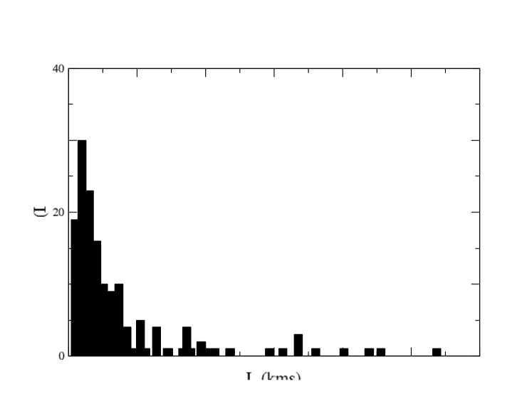
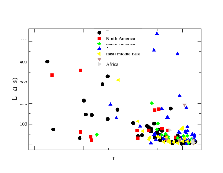
Figure 1: (Top) Histogram of the total length of subway networks. (Bottom) Total length of the network versus first construction date. We grouped the networks according to broad regions.

Concerning the geometry of these networks, as $L$ increases we observe more complex shapes and an increase in the number of lines (see Fig. 2 and also wiki ). Usually for small subways ($L$ of order a couple of 10 kms) we observe a single line or a simple tree (eg. a single line in the case of Baltimore, Haifa, Helsinki, Hiroshima, Miami, Mumbai, Xiamen, …; or many radial lines such as in Atlanta, Bangalore, Incheon, Kyoto, Philadelphia, Rome, Sendai, Warsaw, Boston, Budapest, Buenos Aires, Chicago, Daegu, Kiev, Los Angeles, Sapporo, Tehran, Vancouver, Washington DC). For larger $L$ (of order 100 kms), we typically observe the appearance of a loop line, either in the form of a single ring (e.g.  Glasgow) or multiple lines with connection stations (Athens, Budapest, Lisbon, Munich, Prague, São Paulo, St. Petersburg, Cairo, Chennai, Lille, Marseille, Montreal, Nuremberg, Qingdao, Toronto). For larger networks ($L$ over 200  kms) we observe in general some more complex topological structure (Berlin, Chongqing, Delhi, Guangzhou, Hong Kong, Mexico City, Milan, Nanjing, New York, Osaka, Paris, Shenzhen, Taipei). For the largest networks, convergence to a structure with a well-connected central core and branches reaching out to suburbs has been observed Roth:2012 .

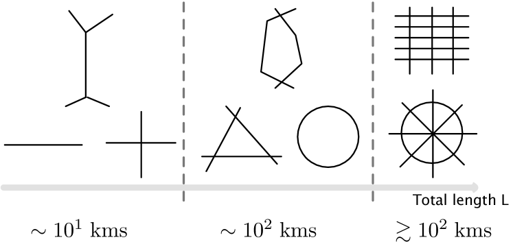
Figure 2: Typical observed shapes when the length $L$ increases. For small $L$ we observe a line or a simple tree. For larger $L$ we observe the appearance of a loop and for much larger $L$ more complex shapes including a lattice like network or a superimposition of a ring and radial lines.

In this paper we investigate the optimal structure of transportation networks, as a function of length $L$, for several related notions of optimal involving minimizing travel time. Real-world subway networks have developed under many other factors, of course, rather than resulting from the optimization of some simple quantity, but optimal structures provide interesting benchmarks for comparison with real-world networks.

There has been extensive study of optimal networks over a given set of nodes (such as the minimum spanning tree Graham:1985 , or other optimal trees Barthelemy:2006 ). Some such problems allow extra chosen nodes, for example the Steiner tree problem Hwang:1992 , or geometric location problems in which $n$ given demand points are to be matched with $p$ chosen supply points Megiddo:1984 . At another extreme is the much-studied Monge-Kantorovich mass transportation problem Rachev:1998 , involving matching points from one distribution with points from another distribution. Our setting is fundamentally different, in that what we are given is just the density of start/end points on the plane. A network is intrinsically one-dimensional, in the sense of being a collection of (maybe curved) lines embedded in the plane. In a sense we are studying a coupling between a given distribution over points in the continuum and a network of our choice constrained only by length and connectedness. Some simpler problems of this type have been addressed previously. For instance, the problem of the quickest access between an area and a given point was discussed in Bejan:1996 ; Bejan:1998 . More recently, the impact of the shape of the city and a single subway line was discussed in Gettrick:2019 . Algorithmic aspects of network design questions similar to ours have been studied within computational geometry (e.g. Okabe:1992 chapter 9) and “location science” (e.g. Laporte:2015 and references therein). But our specific question – optimal network topologies as a function of population distribution and network length – has apparently not been explicitly addressed.

II The model and the main question

Here we define precisely the general model we have in mind, and the three different variants that we will in fact study. Our model makes sense for an arbitrary “population density” $\rho(\ )$ on the plane, but we will study mostly the isotropic (rotation-invariant around the origin) case, in particular the (standard) Gaussian density

$$\rho(x,y)=(2\pi)^{-1}\exp(-r^{2}/2),\ r^{2}=x^{2}+y^{2}$$

and the uniform distribution on a disc. The population density is of individuals who wish to reach as quickly as possible other points in the system (for simplicity we do not distinguish densities of residences and workplaces, for instance). Continuing with the subway interpretation, we assume that one can move anywhere in the plane at speed $1$, and one can move within the network at speed $S>1$ (this quantity can therefore be seen as the ratio $S=v_{s}/v_{w}$ between walking and subway velocities). Note that we envisage each position on the network as a “station” where the subway is accessible – the relative efficiency of two networks would be little affected by the incorporation of discrete stations into a model.

The general problem is the following one. For any pair of points $(z_{1},z_{2})$ in the plane, there is a minimum (over all possible routes) time $\tau(z_{1},z_{2})$ to journey from $z_{1}$ to $z_{2}$, and so the average journey time is

$$\overline{\tau}=\int\int\tau(z_{1},z_{2})\rho(z_{1})\rho(z_{2})\ dz_{1}dz_{2}.$$

This depends on the network. For a given $L$ there is some optimal network of length $L$ (this network also depends on the speed ratio $S$ and on $\rho$). We study the shapes and average journey times for such optimal networks.

This “general model” is very simplistic – as a next step, a companion paper AB2 studies an extended model including a waiting time $W$ whenever we take the subway or connect from one line to another – but nevertheless seems analytically intractable. So in fact we will consider three simpler variants.

First, we will consider the problem of minimizing the average (over starting points from the given distribution) distance to the network, that is to the closest point in the network. Note here that we don’t compute the average time between all pairs of points but just consider the access time to the network from each point. The second variant that we consider is the problem of minimizing the journey time from the points to a single destination, which we may take to be the origin $O$. In the third variant, we engage the general issue of routes between arbitrary points which typically (but not always) involve entering and exiting the subway network, but now require these entrances and exits to be the closest positions to the starting and ending points, rather than the time-minimizing positions.

Except in asymptotic results (e.g. equation (4)) we do not have exact formulas involving optimal networks. Instead we consider a range of simple network shapes, allowing us to investigate the possible shape of optimal networks.

III A first simplification: optimal placement

Here we consider the simplest variant, in which we seek the network (of given length $L$) that minimizes the average distance from a point to the network. This is almost the same as the $S=\infty$ case of the general model, because the journey time between two points would be the sum of the two distances to the network, except that in the general model the shortest route might not use the subway network at all. Intuitively an optimal network must come close to most points of the distribution. Although superficially similar to the notion of space-filling curves Sagan:1994 , the latter are fractal curves whereas our networks (having finite length) cannot have fractal curves.

III.1 Some rigorous results

Here we outline some rigorous results for this variant model, with details to be given in the companion paper AB2 .

Observe that given a straight line segment, the area within a small distance $\varepsilon$ from the line is $2\varepsilon$ per unit length. So in a network of length $L$, the total area within that distance from the network is at most $2\varepsilon\times L$, and is reduced from that value by the presence of curved lines and intersections. By extending that argument one can prove AB2 that the optimal network is always a tree (or a single curve, which is a special case of a tree). For a non-isotropic density $\rho(\ )$ the optimal network may not be a single line, but we conjecture that for isotropic densities decreasing in $r$ the optimal network is always a single curve.

Although $L\to\infty$ asymptotics are hardly realistic in the context of subway networks, the same questions might arise in some quite different context, so it seems worth recording the explicit result for asymptotics. In the $L\to\infty$ limit, the optimal network density (i.e. the edge length per unit area of the network) near point $z$ should be of the form $L\phi(\rho(z))$ for some increasing function $\phi$. By scaling, the average distance from a typical point near $z$ to the network should be $c_{0}/(L\phi(\rho(z)))$ for some constant $c_{0}$. So the overall average distance to the network is

$$\overline{d}(L)=\frac{c_{0}}{L}\int\frac{1}{\phi(\rho(z))}\rho(z)dz.$$ (1)

The total length constraint implies that

$$\int\phi(\rho(z))\ dz=1.$$ (2)

A standard Lagrange multiplier argument shows that the integral in (1) is minimized, over functions $\phi$ under constraint (2), by a function of the form $\phi(\rho)=a\rho^{1/2}$, and then (2) and (1) combine to show

$$\overline{d}(L)_{opt}=\frac{c_{0}}{L}\left(\int\rho^{1/2}(z)\ dz\right)^{2}.$$ (3)

Finally, the constant $c_{0}$ can be re-interpreted as the minimum average-distance-to-network in the context of networks on the infinite plane with network density $=1$. From our initial “area within a small distance $\varepsilon$” observation, the optimal network in the infinite context consists simply of parallel lines spaced one unit apart, for which $c_{0}=1/4$. So this analytic argument shows

$$\overline{d}(L)_{opt}\sim\frac{1}{4L}\left(\int\rho^{1/2}(z)\ dz\right)^{2}\mbox{ as }L\to\infty.$$ (4)

This result makes no assumption about the underlying density $\rho$. In the Gaussian case, the integral in (4) equals $\sqrt{8\pi}$ and so $\overline{d}(L)_{opt}\sim\frac{2\pi}{L}$.

As explained in AB2 , what this argument actually shows is that a sequence of networks is asymptotically optimal as $L\to\infty$ if and only if the rescaled local pattern around a typical position $z$ consists of asymptotically parallel lines with spacing proportional to $\rho^{-1/2}(z)$, but the orientations can depend arbitrarily on $z$. Visualize a fingerprint. For an isotropic density we can arrange such a network to be a spiral. This enables us to check the Gaussian prediction numerically. Consider a spiral of length $L$ starting at some point $(a_{L},0)$ and with rings at radius $r$ separated by $b_{L}\exp(r^{2}/4)$, and then optimize over $(a_{L},b_{L})$. Numerically we find slow convergence toward this limit behavior, shown in Fig. 3.

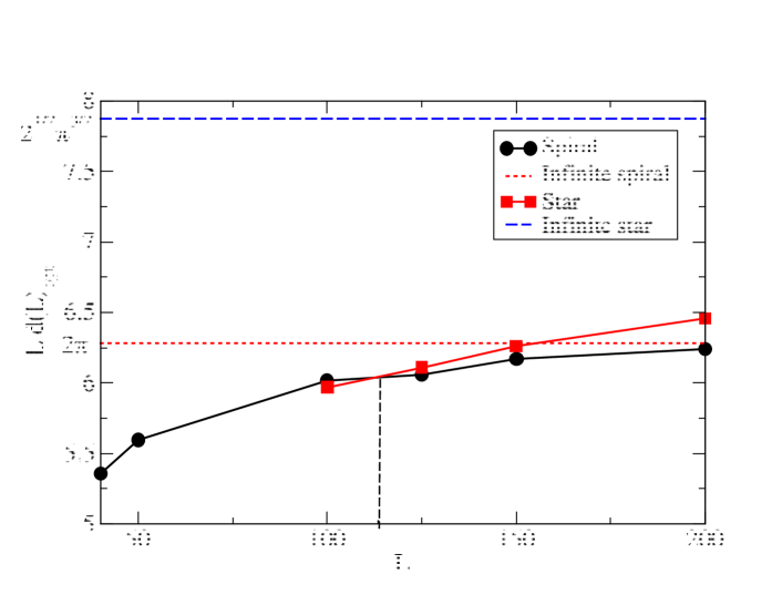
Figure 3: Rescaled average distance $L\overline{d}(L)_{opt}$ versus $L$ for the spiral and the star network. For the spiral, we observe a slow convergence towards the theoretical limit $2\pi$ for gaussian disorder. The convergence is even slower for the star network which converges to $2^{1/2}\pi^{3/2}$. For $L\approx 110$ (dashed vertical line) the spiral outperforms the star network.

III.2 Numerical study: different shapes

Unfortunately the asymptotics above say nothing about the actual shapes of the optimal networks for more realistic smaller values of $L$. Intuitively, we expect that for very small $L$ the optimal network is just a line segment centered on the origin. As $L$ increases we expect a smooth transition from the line segment to a slightly-curved path, a “C-shaped” curve. But then how the optimal shapes transition to a tight spiral path (presumed optimal for very large $L$) is not a priori easy to guess.

We tested 8 shapes numerically for the standard Gaussian distribution. In each shape the length is $L$, and we optimized over any free parameters (such as $s$ in the $2\times 2$ grid).

• The line segment $[-L/2,L/2]$.

• The “cross” (two length $L/2$ lines crossing at the origin).

• The “hashtag” or “$2\times 2$ grid” (Fig. 4(a)).

• The “ring” (circle centered on the origin).

• The “C-shape” (off-centered partial circle, with arc length $2\theta$ removed, see Fig. 4(b)).

• The “S-shape”: two arcs of circle of radius $R$ and of angle $2\theta$, connected by a straight line of length $2R$ (see Fig. 4(c)).

• The “star” with $n_{b}$ branches of length $r^{*}$ (so $r^{*}n_{b}=L$, see Fig. 4(d)).

• The (Archimedean) “spiral”, $r=a\theta+b$.

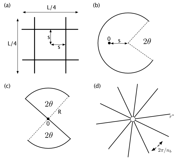
Figure 4: Main shapes studied here (in addition to the line and the spiral). (a) The “hashtag” of $2\times 2$ grid with parameter $s$. (b) The “C-shape” with paramerers $s$ and $\theta$. (c) The “S-shape” with parameter $\theta$. (d) The star network with $n_{b}$ branches of size $r^{*}$.

Recall that the optimal (over all shapes) shape is always a path or tree, so the $2\times 2$ grid or ring can never be overall optimal. Note also that (for any isotropic distribution) the optimal ring has radius equal to the median of the radial component of the underlying distribution, in our Gaussian case $\sqrt{2\log 2}\approx 1.18$.

We simulated these different shapes in the Gaussian disorder case, and for each value of $L$ we optimize over the parameters defining the different shapes. We show the results for these various shapes in Fig. 5.

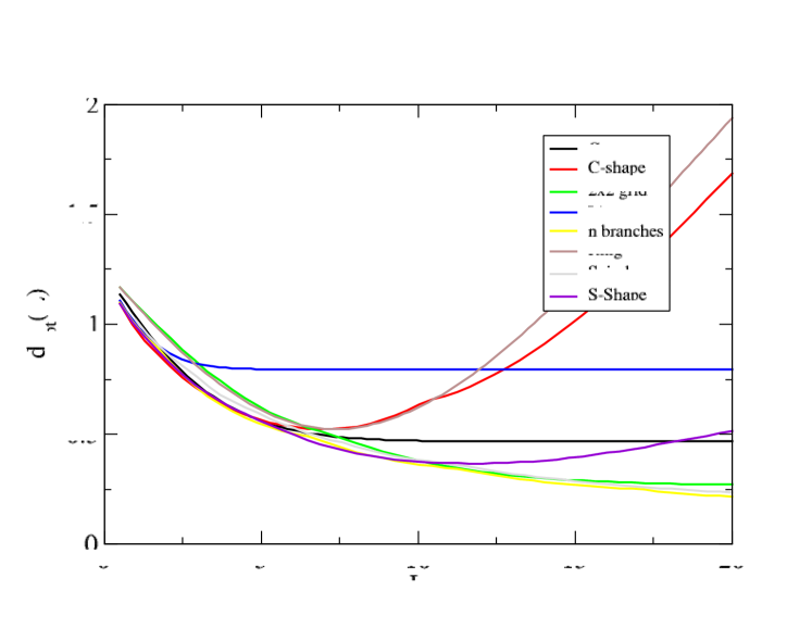
Figure 5: Average distance to the network versus L for various shapes.

The following general picture emerges:

• For small $L\lesssim 3.2$ the optimal shape is the C-shape. We note that for this shape the optimal $\theta$ decreases with $L$: for $L\approx 6$ we have $s=0$ and for $L\approx 8.0$ the optimal $\theta=0$. When $\theta=0$ and $s=0$ we then recover the ring result (see Fig. 6).

  

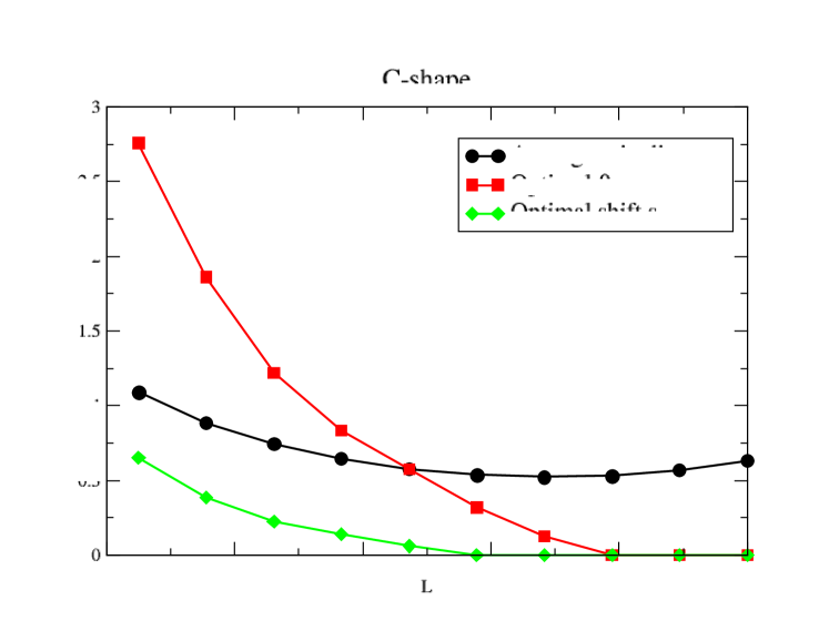
  Figure 6: Study of the C-shape with parameter $s$ and $\theta$.

• For $3.2\lesssim L\lesssim 5.8$, the cross (star network with 4 branches) is optimal.

• For $5.8\lesssim L\lesssim 8.7$, the S-shape is optimal. We note that for this shape, as $L$ increases, the optimal angle $\theta$ increases from $0$ to $\pi/2$, but with a jump at $L\approx 5$ (see Fig.  7).

  

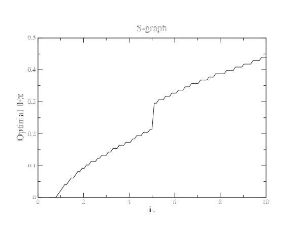
  Figure 7: Study of the S-shape: evolution of the optimal angle $\theta$ versus $L$.

• For $L\gtrsim 8.7$ the star network with $n_{b}$ branches is the optimal shape. The number of branches is roughly increasing with $L$: $n_{b}\sim pL+q$ with $p\approx 0.4$.

• The simple Archimedean spiral was slightly less efficient than the star network over the range of $L$ considered above: For $L=20$, the average time is $\overline{d}_{opt}\approx 0.215$ for the star network, while for the spiral we have $\overline{d}_{opt}\approx 0.233$.

III.2.1 Qualitative discussion

In the examples above, the shapes were not adapted specifically to the Gaussian model (although the numerical parameters were optimized) and so are shapes one might consider for other isotropic distributions. Recall that our previous analysis of the $L\to\infty$ behavior found optimal networks to be spiral-like in a specific distribution-dependent way (near a point $z$, the rings are separated by distance proportional to $(\rho(z))^{-1/2}$). For comparison, it is straightforward to show that the asymptotic behavior of the optimal star shape is $\overline{d}(L)_{opt}\sim 2^{1/2}\pi^{3/2}/L$, and numerical results are shown in the Fig. 3. By comparing with the spiral, we estimate that the value at which such spiral networks out-perform star networks in the Gaussian model is around $L=110$.

Our numerics thus suggest there are 4 sharp transitions of shape: C-shape to cross near $L=3.2$, cross to S-shape near $L=5.8$, S-shape to star near $L=8.7$ and finally a transition from the star network to the spiral near $L=110$. But the star only slightly out-performs these curves, so it is possible that in fact there is a smooth evolution of curves as optimal networks. An alternative numerical approach is to seek the overall optimal network, via simulated annealing for example. This is computationally difficult, but some preliminary results for optimal curves are shown in Fig. 8, and are roughly consistent with our qualitative summary.

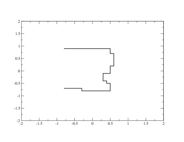
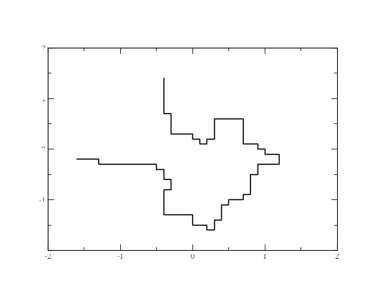
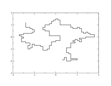
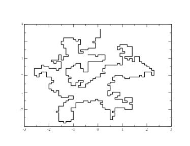
Figure 8: Best configurations obtained with simulated annealing for different values of $L=5,10,20,50$. The simulations are obtained with a lattice polymer and using the pivot algorithm Madras:1988 .

IV The minimum distance to the center

For our second variant, closer to the general problem, we seek the network of length $L$ that minimizes the average time to reach a designated “center” location. This was for example discussed in Bejan:1996 ; Bejan:1998 where the case of street networks was considered and where the optimal tree was found. This problem in the context of a single line bus was also considered in Okabe:1992 (and references therein). With respect to transportation systems such as subways or trains, this is obviously a crude simplification as we are in general interested in reaching many other stations and not a single location. As we will see in the rest of the paper, our results suggest that this simplified problem perhaps captures the essence of the general problem and might constitute a useful toy model where analytical calculations are feasible. As in our other variants we envisage each position on the network as a “station” where the subway is accessible.

Taking as before an isotropic density $\rho(\ )$ and the origin as “center”, we seek the “optimal” network that minimizes

$$\overline{\tau}=\int\tau(z,0)\rho(z)dz$$ (5)

where $\tau(z,0)$ is the minimum time to go from the point $z$ to the origin $0$. The optimal network will depend on the parameter $S=v_{s}/v_{w}>1$, where $v_{s}$ is the speed within the network, and $v_{w}$ the speed outside.

In order to simplify analytical calculations we assume in this variant that the paths from the points to the network can be made only along circular ($r=\mathrm{const.}$) or radial ($\theta=\mathrm{const.}$) lines. It remains true that the overall optimal network must be a path or tree. Indeed, if there is a circuit in the network, there is at least one point such that starting in either direction takes the same time to get to the center. One can then remove a small interval from that point, and re-attach elsewhere to get a better network.

However we will consider only simple shapes for the network, starting from the star network and then adding a ring to it. As we will see below, for these structures we can develop simple analytical calculations and observe important phenomena such as a topological transition.

IV.1 Star network

We again consider the star network, having $n_{b}$ branches of lengths $r^{*}$, outward from the origin, evenly spaced with angle $2\pi/n_{b}$ spacing (see Fig. 4(d)). So $L=n_{b}r^{*}$ and (for given $L$) $n_{b}$ is a free parameter to be optimized over. By isotropy we can write

$$\rho(x,y)=\rho(r)\mbox{ for }r^{2}=x^{2}+y^{2}.$$

Again by isotropy, the average time $\overline{\tau}$ to the center is such that

$$\frac{1}{2n_{b}}\overline{\tau}= \int_{0}^{\pi/n_{b}}\mathrm{d}\theta\Big{[}\int_{0}^{r^{*}}\mathrm{d}rr\rho(r)(\frac{\theta r}{v_{w}}+\frac{r}{v_{s}})$$

$$+\int_{r^{*}}^{R}\mathrm{d}rr\rho(r)(\frac{r-r^{*}}{v_{w}}+\frac{\theta r^{*}}{v_{w}}+\frac{r^{*}}{v_{s}})\Big{]}.$$ (6)

In the following we will consider the uniform density on a disc, and an exponentially decreasing density.

IV.1.1 Uniform density

Here we take the uniform density $\rho(r)=\rho_{0}=1/(\pi R^{2})$ on a disk of radius $R$. Without the network the average time to reach the center is $\tau_{0}=2R/(3v_{w})$. Write $\eta=1/S=v_{w}/v_{s}$, and assume that taking the subway is always better than walking directly to the center, which is the condition that $\eta\leq 1-\pi/n_{b}$. Write $u^{*}=r^{*}/R$ (the branch length relative to city radius) and $u_{0}=L/R$ (network length relative to city radius) and $\chi=\pi/n_{b}$. Evaluating the integrals in (6), the average time $\overline{\tau}$ to reach the center via subway satisfies

$$\frac{\overline{\tau}}{\tau_{0}}= \frac{u^{*3}}{2}[-\frac{\chi}{2}-\eta+1]$$

$$-\frac{3}{2}u^{*}[-\frac{\chi}{2}-\eta+1]+1.$$ (7)

For given $L$ we want to optimize over the free parameter $r^{*}$, that is over $u^{*}$. From $L=n_{b}r^{*}$ we obtain $\chi=\pi u^{*}/u_{0}$ and then the average time as a function of $u^{*}$ reads

$$\frac{\overline{\tau}}{\tau_{0}}=\frac{1}{2}(u^{*3}-3u^{*})[-\eta+1-\pi\frac{u^{*}}{u_{0}}]+1.$$ (8)

Minimizing this quantity over $u^{*}$ leads to a polynomial of degree 3, and the behavior of the solution is shown numerically in Fig. 9.

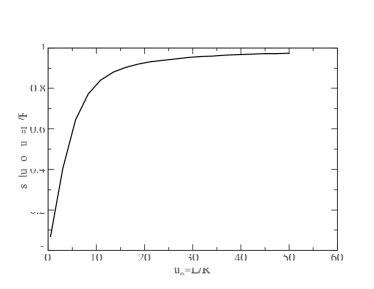
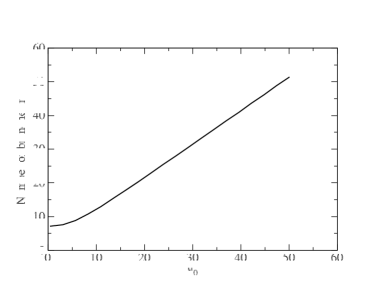
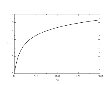
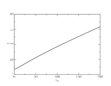
Figure 9: We show here the result of the minimization of the average time for the star network with parameters $n_{b}$ and $r^{*}$ with the constraint $L=n_{b}r^{*}$. On the left we show the length of branches $r^{*}$ versus $u_{0}=L/R$ and on the right the number of branches $n_{b}$ versus $u_{0}$ (here $\eta=1/8$). The top row corresponds to the uniform density case and the bottom one to the exponential density.

As is intuitively obvious, for large $u_{0}=L/R$ it is optimal to use roughly $u_{0}$ branches of length almost $R$; more precisely for $u_{0}\gg 1$ we obtain

$$\begin{cases}u^{*}&=1-\frac{\pi}{3(1-\eta)u_{0}}+{\cal O}(\frac{1}{u_{0}^{2}})\\ n_{b}&=u_{0}+{\cal O}(1).\end{cases}$$ (9)

Perhaps less obvious is the initial behavior over $0\leq u_{0}\leq 10$, where the length of branches is increasing faster than their number. In other words we first observe a radial growth and then an increase of the number of branches.

IV.1.2 Exponential density

In this case, we take the density of the radial component to be $\rho_{0}r\mathrm{exp}(-r/r_{0})$ on the infinite plane. Without the network the average time to reach the center is $\tau_{0}=2r_{0}/v_{w}$. Evaluating the integrals in (6), the average time $\overline{\tau}$ to reach the center via subway satisfies

$$\frac{\overline{\tau}}{\tau_{0}} =\frac{\pi u^{*}}{2u_{0}}+\eta$$

$$-\mathrm{e}^{-u^{*}}\left(\frac{\pi u^{*}}{u_{0}}+\eta-1\right)\left(\frac{u^{*}}{2}+1\right)$$ (10)

where $u^{*}=r^{*}/r_{0}$ and $u_{0}=L/r_{0}$. We can plot this function and look numerically for the minimum. The results are shown in Fig. 9 (bottom).

We observe here that for large resources ($u_{0}\gg 1$) the number of branches scales as $n_{b}\sim au_{0}$ with $a\approx 0.1$ and the solution $u^{*}$ seems to converge slowly to some value that depends on $\eta$.

IV.2 Loop and branches

We now consider a more interesting case where we have $n_{b}$ branches of length $r^{*}$ and a ring of radius $\ell$ (see Fig. 10). This case is essentially motivated by subway networks that seem to display this type of structure when they are large enough Roth:2012 .

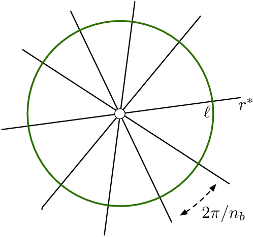
Figure 10: Schematic of the star network combined with a ring. We have now three parameters: the number of branches $n_{b}$, the length $r^{*}$ of the branches, and the radius $\ell$ of the ring.

We have 3 parameters: $n_{b}$, $\ell$ and $r^{*}$, where $\ell\leq r^{*}$ for connectivity. The total length of the network is

$$L=2\pi\ell+n_{b}r^{*}.$$ (11)

This network enables us to study the relative contributions of loop and branches to our goal of minimizing the average time to go to the center. This case is analytically difficult, so we study it numerically with a simulation.

We first consider the uniform distribution on a disc of radius $r_{0}$, and again choose $\eta=1/8$ (which corresponds to the reasonable values $v_{w}\approx 5$km/h and $v_{s}\approx 40$km/h). We first study the case where $n_{b}$ is fixed and where we optimize the network over $r^{*}$ and $\ell$. In Fig. 11, we show the results for the optimal value of $r^{*}$ and $\ell$ versus $u_{0}=L/r_{0}$ normalized by $n_{b}$.

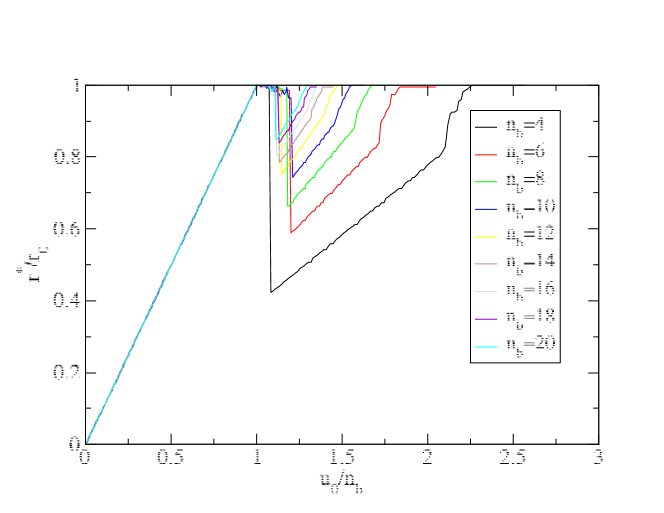
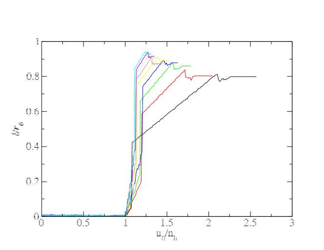
Figure 11: Uniform density: results for the star+loop network for different values of $n_{b}$. (Top) Normalized radius of the ring. (Bottom) Normalized length of branches. We normalized $u_{0}$ by $n_{b}$ in order to get the same “transition” point at $u_{0}/n_{b}=1$. These results are obtained for $\eta=1/8$.

We observe that when resources are growing from $0$, we have only a radial network ($\ell=0$). At $u_{0}/n_{b}=1$ we have a “transition” point where a loop appears. This means that until $u_{0}=n_{b}$ all the available resource is converted into the radial structure. When the radial structure is at its maximum ($r^{*}=r_{0}$) we observe the appearance of a loop whose diameter is then increasing with $u_{0}$.

We note that even if both the number of branches and the size of the loop undergo a discontinuous transition, the average minimum time displays a smooth behavior. Also, if we increase further the total length $L$, it will result in a larger number of branches $n_{b}$.

In the uniform density case, the domain is finite (a disk of radius $R$) and at fixed value of $n_{b}$, there is therefore a maximum value of $L_{max}=n_{b}R+2\pi R$. For larger values of $L$, the optimal network will increase its number of branches $n_{b}$. It is different in the Gaussian disorder case: the domain is infinite and there is no obstacle to have a fixed value of $n_{b}$ with size $r^{*}$ growing indefinitely with $L$. We can thus expect some differences with the uniform density case. We repeated the calculations above for $100$ configurations and the average together with the results for each configuration are shown in Fig. 12.

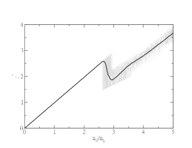
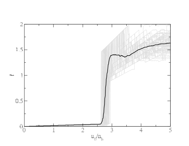
Figure 12: Gaussian density ($\sigma=1$): results for the star+loop network for $n_{b}=8$. (Top) Size $r^{*}$ of the branches. (Bottom) Radius of the ring. These results are averaged over $100$ configurations and are obtained for $\eta=1/8$. The grey curves represent the results for each configuration.

We still observe the different regimes separated by an abrupt transition: the first regime where the size of branches grows with $L$ and the second regime where there is a ring whose size grows very slowly with $L$. In contrast with the uniform density case, the transition takes place for a value $u_{0}/n_{b}$ that fluctuates in the range $[2.5,3.0]$.

V The general model

As discussed in the introduction, we will now consider the “general” setting of routes between arbitrary points $z_{1}$ and $z_{2}$. The route can either go straight (speed $v_{w}$) from $z_{1}$ to $z_{2}$ without using the network, or go $z_{1}\to A_{1}\to A_{2}\to z_{2}$, where $A_{1}$ and $A_{2}$ are “stations” (any points on the network) and where travel from $A_{1}$ to $A_{2}$ is within the network at speed $v_{s}$, and the other journey segments are straight at speed $v_{w}$. In a companion paper AB2 we study the more realistic model where the route is optimized over choice of $A_{1}$ and $A_{2}$, but here we take each $A_{i}$ as the closest station to $z_{i}$. Unlike previous cases, the overall optimal network is not necessarily a tree.

V.1 Various shapes

We present results for various simple shapes, for the standard Gaussian density. We start with the line segment and the ring and the results for different values of $S$ are shown on Fig. 13.

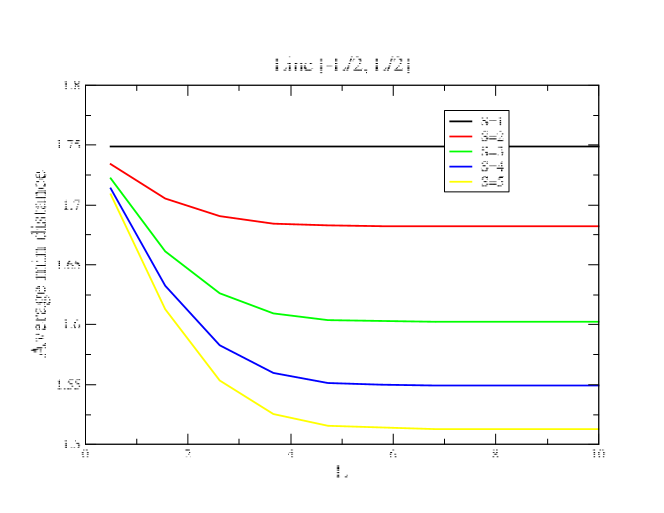
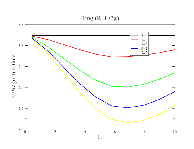
Figure 13: Average journey time in the Gaussian case for different values of $S$ and for (Top) a line and (Bottom) a ring.

For these two shapes, we observe the same behavior as in the time to center problem: for the line there is a quick saturation to a constant, and for the ring there is a minimum at $L\approx 2\pi\sigma$.

We also consider the case of the star network with $n_{b}$ branches and the result is shown on Fig. 14.

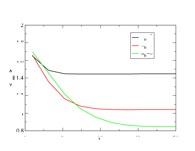
Figure 14: Average journey time (in the Gaussian case) for star networks with different number of branches ($n_{b}=2,4,6$).

We observe that for $0<L\lesssim 1.15$ the line is optimal. For $1.15\lesssim L\lesssim 6.6$, the cross $n_{b}=4$ is the optimal choice, while for $L\gtrsim 6.6$, the solution $n_{b}=6$ is better. Very likely we will have (as in the previous case of the average time to the center) an optimal network with $n_{b}\propto L$.

V.2 Loop and branches: Scaling of the average time

We focus here on the case where the network is made of $n_{b}$ branches of length $r^{*}$ and a loop of radius $\ell$. So $L=n_{b}r^{*}+2\pi\ell.$ We take $n_{b}$ and $\ell$ as the 2 free parameters over which we will minimize the average time. The optimized average time $\overline{\tau}_{min}$ for different values of $S$ is shown in Fig. 15.

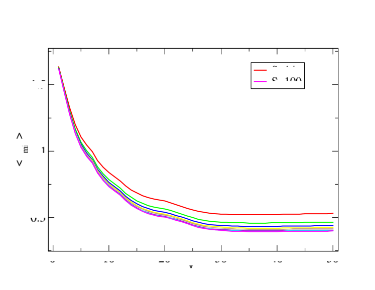
Figure 15: Average time (Gaussian density) for $n_{b}$ branches plus a loop for values of $S$ from $14$ to $100$.

Naively one expects that this quantity behaves as

$$\overline{\tau}_{min}=\frac{a}{\sqrt{L}}+\frac{b}{S}$$ (12)

where the first term of the r.h.s. corresponds to the average distance to the network and which we expect to scale as $1/\sqrt{L}$. The second term corresponds to the shortest path distance within the network. In principle $a$ and $b$ could depend on $L$. If we assume this form to be correct then $S\overline{\tau}_{min}$ versus $X=S/\sqrt{L}$ should be a straight line. We tested this assumption on the data from Fig. 15 and the result is shown in Fig. 16.

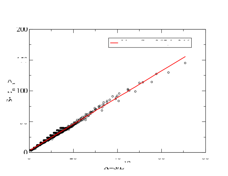
Figure 16: Rescaled average time $S\overline{\tau}_{min}$ versus the rescaled variable $S/\sqrt{L}$.

This good collapse (except for deviations observed for large values of $S/\sqrt{L}$ supports the assumption (12).

V.3 Loop and branches: A topological transition

Still in the branches and loop model, we observe (Fig. 17) a transition: $r^{*}$ grows almost steadily with $\ell=0$, until a transition value at $L_{c}\approx 20$ where the ring appears.

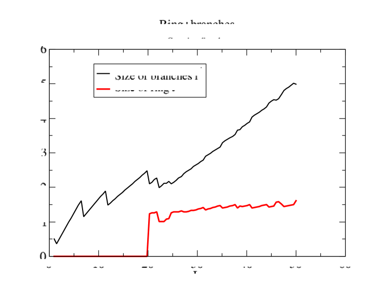
Figure 17: Optimal length of branches and optimal size of the loop versus the total length $L$ (for gaussian disorder): typical shape for $r^{*}$ and $\ell$. As in the case of the quickest path to the origin, we observe a sharp transition for $L\approx 20\sigma$ where a loop of radius $\ell\approx\sigma$ appears (here $\eta=1/2$).

Although the structure changes abruptly it is interesting to note that there is no discontinuity in the average minimum time. The size of the ring stays stable with $\ell\approx\sigma$ (the Gaussian s.d.). Naively, we can say that the ring appears when the branches can have a length $r^{*}\approx\sigma$ and a loop of size $\ell\approx\sigma$ which gives the condition $L_{c}\approx n_{b}\sigma+2\pi\sigma$. At the transition, we observe that we have $n_{b}\approx 8$ which then gives $L_{c}\approx 14$, not too far from the value $L_{c}=20$ observed here.

The quantity $L_{c}$ is independent from $S$ which is expected, as it is essentially controlled by the topology of the network. We note that this transition was already observed in the previous case “minimum distance to the center”. As $L$ increases the optimal number of branches grows roughly from $2$ to $10$. The picture that emerges here is consistent with the empirical study Roth:2012 : we observe a ring around the “core” of the city and then branches radiating from it. More generally, these results suggest that the distance to center problem is a reasonably good proxy for the more general problem.

VI Discussion

Algorithmic aspects of network design questions similar to ours have been studied within computational geometry (e.g. Okabe:1992 chapter 9) and “location science” (e.g. Laporte:2015 ). But our specific question – optimal network topologies as a function of population distribution and network length – has apparently not been explicitly addressed. Although real-world networks are probably not optimal and result from the superimposition of many different factors, understanding theoretically optimal networks could give some information about the actual structure observed in many cases. For example, it could help us to understand the seemingly universal structure displayed by very large subway networks Roth:2012 .

Even for simple models, optimizing over all possible topologies is difficult, so we investigated only various simple shapes. We provided general arguments and analytical calculations in simple cases and most of our analysis is numerical. In general we expect an evolution of the shape of optimal networks when $L$ increases, with the possible existence of sharp transitions between different shapes. Although we weren’t able to prove this in general, we observed such transitions in simple cases such as branches and a loop: in the case of Gaussian (variance $\sigma^{2}$) population density, starting from a small value of $L$ the branches first grow smoothly, then suddenly for a value $L_{c}$ we observe the appearance of a loop of size $\ell\sim\sigma$. This transition also exists in the case of uniform density.

It would be interesting to see these transitions of overall optimal networks obtained numerically, and this might be feasible in some cases with a simulated annealing type of algorithm. In any case these problems suggest theoretical questions and practical applications which certainly deserve further studies.

References

- (1) Xie F, Levinson D (2011) Evolving transportation networks (Springer Science Business Media).
- (2) Roth C, Kang S, Batty M, Barthelemy M (2012). A long-time limit for world subway networks. Journal of The Royal Society Interface, rsif20120259.
- (3) Barthelemy M (2018) Morphogenesis of Spatial Networks (Springer).
- (4) Bottinelli A, Gherardi M, Barthelemy M (2019) Efficiency and shrinking in evolving networks. arXiv:1902.06063.
- (5) Tero A, Takagi S, Saigusa T, Ito K, Bebber DP, Fricker MD, Yumiki K, Kobayashi R, Nakagaki T (2010) Rules for biologically inspired adaptive network design. Science 327:439.
- (6) Latty T, Ramsch K, Ito K, Nakagaki K, Sumpter DJ, Middendorf M, Beekman M (2011) Structure and formation of ant transportation networks. Journal of The Royal Society Interface 8:1298.
- (7) Perna A, Granovskiy B, Garnier S, Nicolis SC, Labédan M, Theraulaz G, Fourcassié V, Sumpter DJT (2012) Individual rules for trail pattern formation in Argentine ants (Linepithema humile). PLoS Computational Biology 8:2592.
- (8) Ma Q, Johansson A, Tero A, Nakagaki T, Sumpter DJT (2013) Current-reinforced random walks for constructing transport networks. Journal of The Royal Society Interface 10:20120864.
- (9) Bottinelli A, van Wilgenburg E, Sumpter DJT, Latty T (2015) Local cost minimization in ant transport networks: from small-scale data to large-scale trade-offs. Journal of The Royal Society Interface 12:20150780.
- (10) Latora V, Marchiori M (2002) Is the Boston subway a small-world network?. Physica A, 314(1-4):109-13.
- (11) Lee K, Jung WS, Park JS, Choi MY (2008) Statistical analysis of the Metropolitan Seoul Subway System: Network structure and passenger flows. Physica A, 387(24):6231-4.
- (12) Derrible S, Kennedy C (2010) Characterizing metro networks: state, form, and structure. Transportation, 37:275.
- (13) Derrible S (2012) Network centrality of metro systems. PloS one, 6;7(7):e40575.
- (14) Louf R, Roth C, Barthelemy M. Scaling in transportation networks. PLoS One. 2014 Jul 16;9(7):e102007.
- (15) Wikipedia page on rapid transit. https://en.wikipedia.org/wiki/Rapid_transit Accessed 2019.
- (16) Graham RL, Hell P. On the history of the minimum spanning tree problem. Annals of the History of Computing. 1985 Jan;7(1):43-57.
- (17) Barthelemy M, Flammini A (2006) ‘Optimal traffic networks’. Journal of Statistical Mechanics: Theory and Experiment, 24;2006(07):L07002.
- (18) Hwang FK, Richards DS, Winter P. The Steiner tree problem. Elsevier; 1992.
- (19) Megiddo, Nimrod, and Kenneth J. Supowit. ”On the complexity of some common geometric location problems.” SIAM journal on computing 13.1 (1984): 182-196.
- (20) Rachev A and Rüschendorf L. (1998). Mass transportation problems. Vol. I. (Springer)
- (21) Bejan A (1996). Street network theory of organization in nature. Journal of Advanced Transportation, 30(2), 85-107.
- (22) Bejan, A., and G. A. Ledezma. ‘Streets tree networks and urban growth: optimal geometry for quickest access between a finite-size volume and one point.’ Physica A: Statistical Mechanics and its Applications 255.1-2 (1998): 211-217.
- (23) Mc Gettrick M (2019) ‘The role of city geometry in determining the utility of a small urban light rail/tram system’. arXiv:1902.02344.
- (24) Okabe A, Boots B, Sugihara K, Chiu SN (1992). Spatial Tessellations: Concepts and Applications of Voronoi Diagrams. (Wiley)
- (25) Laporte G and Mesa J. The Design of Rapid Transit Networks. In Location Science (Springer) pp. 581–594.
- (26) Sagan H (1994). Space-filling curves. (Springer)
- (27) Aldous D and Barthelemy M. In preparation.
- (28) Madras, Neal and Alan D. Sokal, The pivot algorithm: A highly efficient Monte Carlo method for the selfavoiding walk, J. Stat. Phys. 50 (1988), 109–186.