Properties of a potential energy matrix in oscillator basis

Abstract

Matrix elements of potential energy are examined in detail. We consider a model problem - a particle in a central potential. The most popular forms of central potential are taken up, namely, square-well potential, Gaussian, Yukawa and exponential potentials. We study eigenvalues and eigenfunctions of the potential energy matrix constructed with oscillator functions. It is demonstrated that eigenvalues coincide with the potential energy in coordinate space at some specific discrete points. We establish approximate values for these points. It is also shown that the eigenfunctions of the potential energy matrix are the expansion coefficients of the spherical Bessel functions in a harmonic oscillator basis. We also demonstrate a close relation between the separable approximation and $L^{2}$ basis (J-matrix) method for the quantum theory of scattering.

1 Introduction

Last decades, the methods which involve square-integrable bases for solving scattering problems become popular. In atomic physics such a method is called the J-matrix method [1, 2] and in nuclear physics it is known as the algebraic version of the resonating group method [3, 4]. There are two most popular sets of basis functions which are used to tackle scattering problems. One of them is the basis of oscillator functions, the other is the Slater (Laguerre) basis. The key element of the J-matrix method is that the asymptotic or reference Hamiltonian can be represented by a tridiagonal matrix (the Jacobi matrix) in the discrete representation ([1, 2]). The asymptotic Hamiltonian could be treated analytically and it provides us with two linearly independent solutions, much like the coordinate representation. These are the regular and irregular solutions or incoming and outgoing waves. Thus there is a full correspondence and consistency with the scattering theory in the coordinate representation. Basic ideas of the J-matrix method and its applications to physical problems in different branches of the quantum physics are outlined in a collection of papers Ref. [5].

Discretization is widely used in many-body quantum physics. There are different types of discretization. For example, it is possible to solve linear differential, integral and integro-differential equations by involving a set of discrete points and reducing these equations to a system of linear algebraic equations. Alternatively, one can expand the wave function or its part (for example, internal part) over a set of basis functions selected by physical or computational reasons. In this case, one also arrives to a set of homogeneous or nonhomogeneous equations. If boundary conditions have to be implemented, this set of equations becomes nonhomogeneous. Implementation of boundary condition can be made in the discrete representation (the J-matrix method) or in the coordinate representation (the R-matrix method [6]).

The essence of the J-matrix method is that it is the matrix form of quantum mechanics with correct boundary conditions both for bound states and for scattering states. Within this method the well-known boundary conditions  in coordinate space were transformed to the discrete space of basis functions. Heller and Yamani [1], Yamani and Fishman [2] demonstrated that the oscillator basis yields the tridiagonal or Jacobi form of a reference Hamiltonian for neutral particles, while the Laguerre basis produces the tridiagonal form for the charged particles. The Laguerre basis has been intensively employed for solving three-body problems in nuclear ([7, 8]) and atomic physics ([9, 10]).

The simple relation between expansion coefficients and wave function in coordinate space has been established within the algebraic version of the resonating group method. It was shown in Refs. [3, 4] that the expansion coefficients are proportional to the wave function at discrete points of coordinate space. In Ref. [11], this relation helped to formulate a simple but reliable method of investigating reactions with charged particles by using the oscillator basis. In Ref. [12] the boundary conditions for three particles in continuum were formulated, which allowed the application of the algebraic version of the resonating group method for studying loosely bound states of nuclei with a large excess of neutrons or protons [13], resonance states and reactions in three-cluster continuum of light nuclei [14].

It was also shown that the J-matrix method is equivalent to the R-matrix method [6]. It was demonstrated that the J-matrix method provides a self-consistent realization of the R-matrix method. This relationship is discussed in the Foreword of the book [5] where one can find necessary references. Being applied to the same system, the J-matrix method and R-matrix method give a very close or identical (with the precision of numerical procedures involved) results. Detailed historical review, the explanation of the main ideas and modern development of the R-matrix method are presented in Ref. [15].

Baye and coworkers developed the microscopic R-matrix method [16] which is based on the generator coordinate method. The discrete form of the integral Hill-Wheeler equation is used to determine a wave function in the internal region. The eigenvalues and eigenfunctions of this equation are employed to find a total wave function and the scattering parameters (elements of the R- or S-matrices) in accordance with the R-matrix methodology. This method has been successfully used to study dynamics of many-cluster systems [17].

It is worthwhile noticing another discretization scheme which is supplementary to the above mentioned schemes and is known as the Lagrange-mesh method. The review of the method is given in Ref. [18]. Within this method the Schrödinger equation is presented in a grid of mesh-points generated by the Gauss-quadrature approximation. The Gauss quadrature relates on the properties of the Lagrange polynomials and provides the efficient and reliable solutions of the Schrödinger equation. As will be seen below, the Lagrange-mesh method overlaps with the J-matrix method as they both employ the polynomials to expand the wave function to be determined.

The main differences between Lagrange-mesh method and our realization of J-matrix method are the following (i) we do not use an approximate expression for the kinetic energy operator and (ii) we obtain a different approximate form of matrix elements of the potential energy operator. The latter will be demonstrated in analytical and numerical forms.

It is also important to mention Refs. [19, 20, 21] where a rigorous analysis has been performed to study properties of the tridiagonal equations. This analysis gave a mathematical justification of the J-matrix method by showing the coincidence of not only the spectra of the original Hamiltonian and the tridiagonal matrix but also their spectral measures. In these publications a tridiagonalizing scheme is extended for a more general case of differential, difference and q-difference operators using orthogonal polynomials.

Despite numerous publications on the essence of the J-matrix method and its applications for solving model and real quantum mechanical problems, we believe that there is a gap in studying properties of the potential energy matrix. This matrix is a key ingredient of the J-matrix method and it determines dynamic properties of a system under consideration. Thus our aim is to study the main properties of the potential energy matrix in order to fill in this gap. In the present paper, we deal with a model problem. We consider a particle in a field of a central-symmetric potential in three-dimensional space. In what follows we demonstrate that the model problem reveals some very interesting properties of the potential energy matrix, which can be a help in understanding the properties of the matrix for real nuclear systems. In particular, the results obtained in this paper could open an effective and pictorial way for studying the effect of the Pauli principle on the potential energy of cluster systems.

The present paper is the first one in a series of papers which are devoted to studying properties of potential energy matrices in different many-body systems. In these papers we are going to study (i) model two-body problems (the present paper), (ii) two-cluster systems and (iii) three-cluster systems. As will be shown below, one of the important outcomes of the present paper is that diagonalization of the matrix of the potential energy operator suggests a natural way of obtaining the local form for the nonlocal operator.

The paper is organized as follows. In Sec. 2 we introduce tools for investigating properties of the potential energy matrix and all the main ingredients of the present calculations. In this Section we also formulate propositions which predict the structure of eigenvalues and eigenfunctions of the matrix. In Sec. 3 we discuss results of numerical calculations for four potentials and verify the predictions made in the previous Section. We give our final remarks and summarize the most important conclusions in Sec. 4.

2 Method

2.1 Potential energy

In this Section, we consider an operator of potential energy and its matrix elements between oscillator functions. As was pointed out above, we deal with a local (in coordinate space) potential $\widehat{V}\left(r\right)$. In momentum space this potential has a nonlocal form:

$$\widehat{V}_{L}\left(p,\widetilde{p}\right)=\frac{2}{\pi}\int_{0}^{\infty}drr^{2}j_{L}\left(pr\right)\widehat{V}\left(r\right)j_{L}\left(\widetilde{p}r\right),$$ (1)

where $j_{L}\left(x\right)$ is a spherical Bessel function (see Section 10 of the book [22]). Moreover, its shape depends on the orbital momentum $L$.

We consider matrix elements of the potential energy operator $\widehat{V}\left(r\right)$ between oscillator functions $\left|n\right\rangle=\Phi_{n}\left(r,b\right)$ in coordinate space or the nonlocal operator $\widehat{V}_{L}\left(p,\widetilde{p}\right)$ between oscillator functions $\left|n\right\rangle=\Phi_{n}\left(p,b\right)$ in momentum space, where

$$\Phi_{nL}\left(r,b\right) = \left(-1\right)^{n}N_{nL}~{}b^{-3/2}\rho^{L}e^{-\frac{1}{2}\rho^{2}}L_{n}^{L+1/2}\left(\rho^{2}\right),\quad\rho=\frac{r}{b},$$ (2)

$$\Phi_{nL}\left(p,b\right) = N_{nL}~{}b^{3/2}\rho^{L}e^{-\frac{1}{2}\rho^{2}}L_{n}^{L+1/2}\left(\rho^{2}\right),\quad\rho=pb,$$ (3)

$b$ is the oscillator length, $n$ is the number of radial quanta and normalization constant $N_{nL}$ is defined by the following expression

$$N_{nL}=\sqrt{\frac{2\Gamma\left(n+1\right)}{\Gamma\left(n+L+3/2\right)}}.$$

One immediately notices the similarity of the oscillator functions in the coordinate and momentum spaces, as they have the same dependence on the dimensionless variable $\rho$. This reflects the similarity of the oscillator Hamiltonian in coordinate and momentum spaces. The oscillator functions are known to be related by the integral transformations.

$$\Phi_{nL}\left(p,b\right) = \sqrt{\frac{2}{\pi}}\int_{0}^{\infty}drr^{2}j_{L}\left(pr\right)\Phi_{nL}\left(r,b\right),$$ (4)

$$\Phi_{nL}\left(r,b\right) = \sqrt{\frac{2}{\pi}}\int_{0}^{\infty}dpp^{2}j_{L}\left(pr\right)\Phi_{nL}\left(p,b\right).$$ (5)

These relations can be treated in the following way. The oscillator functions $\Phi_{nL}\left(p,b\right)$ in the momentum space are the expansion coefficients of the spherical Bessel function in the oscillator functions $\Phi_{nL}\left(r,b\right)$ in the coordinate space, and vice versa. Recall that the spherical Bessel function $j_{L}\left(pr\right)$ is also a wave function of free motion of a particle with a fixed value of the orbital momentum $L$ and the wave number $p$. This assertion can be formulated as

$$\sqrt{\frac{2}{\pi}}j_{L}\left(pr\right)=\sum_{n=0}^{\infty}\Phi_{nL}\left(p,b\right)\Phi_{nL}\left(r,b\right),$$ (6)

which reflects the peculiarity possessed by the oscillator basis only. Another important property of the oscillator functions, which will be employed in the present paper, is associated with the completeness relation

$$\sum_{n=0}^{\infty}\Phi_{nL}\left(x,b\right)\Phi_{nL}\left(\widetilde{x},b\right)=\delta\left(x-\widetilde{x}\right).$$ (7)

Such a relation is valid for any orthonormal basis of square-integrable functions. This relation shows us that the expansion coefficients of the delta function (or a wave function of a free motion in the momentum space $x=p$) in oscillator functions are also oscillator functions.

We have to mention the last important property of oscillator functions which is useful in explaining our results. An oscillator function $\Phi_{nL}\left(x,b\right)$ has $n$ nodes in the region $0\leq\rho\leq R_{n}$, where

$$R_{n}=\sqrt{4n+2L+3}$$ (8)

is a turning point of the classical oscillator with the energy

$$E_{n}=\frac{\hbar^{2}}{mb^{2}}\left(2n+L+\frac{3}{2}\right).$$

The oscillator function has a negligibly small value in the classically forbidden region $\rho>R_{n}$ due to the factor $e^{-\rho^{2}/2}$ in Eqs. (2) and (3). By this reason a set of $N$ oscillator functions can approximate a wave function only in the range $0\leq\rho\leq R_{N}$.

Note that the matrix elements of the potential energy operator calculated between the oscillator functions in coordinate space are identical to those, which are calculated in momentum space.  The potential energy matrix

$$\left\langle nL\left|\widehat{V}\right|mL\right\rangle = \int_{0}^{\infty}drr^{2}\Phi_{nL}\left(r,b\right)\widehat{V}\left(r\right)\Phi_{mL}\left(r,b\right),$$ (9)

$$= \int_{0}^{\infty}dpp^{2}\int_{0}^{\infty}d\widetilde{p}\widetilde{p}^{2}\Phi_{nL}\left(p,b\right)\widehat{V}_{L}\left(p,\widetilde{p}\right)\Phi_{mL}\left(\widetilde{p},b\right)$$ (10)

approximates the exact potential $\widehat{V}\left(r\right)$ ($\widehat{V}\left(p,\widetilde{p}\right)$) by the following expression

$$\widehat{V}_{N}\left(r,\widetilde{r}\right) = \sum_{n,m=0}^{N-1}\Phi_{nL}\left(r,b\right)\left\langle nL\left|\widehat{V}\right|mL\right\rangle\Phi_{mL}\left(\widetilde{r},b\right),$$ (11)

$$\widehat{V}_{N}\left(p,\widetilde{p}\right) = \sum_{n,m=0}^{N-1}\Phi_{nL}\left(p,b\right)\left\langle nL\left|\widehat{V}\right|mL\right\rangle\Phi_{mL}\left(\widetilde{p},b\right),$$ (12)

which in limiting case $N\rightarrow\infty$ coincides with the original exact form:

$$\lim_{N\rightarrow\infty}\widehat{V}_{N}\left(r,\widetilde{r}\right) = \delta\left(r-\widetilde{r}\right)\widehat{V}\left(r\right),$$

$$\lim_{N\rightarrow\infty}\widehat{V}_{N}\left(p,\widetilde{p}\right) = \widehat{V}_{L}\left(p,\widetilde{p}\right).$$

As we can see, the oscillator basis realizes a specific form of separable potentials.

Suppose we constructed $N\times N$ matrix of the operator $\widehat{V}$.  This matrix can be reduced to the diagonal form. Let us use notations $\lambda_{\alpha}$ for eigenvalues and $\left\{U_{n}^{\alpha}\right\}$ for the corresponding eigenvectors. The latter form an orthogonal matrix $\left\|U\right\|$. The eigenvectors define new eigenfunctions

$$\phi_{\alpha}\left(r,b\right) = \sum_{n=0}^{N-1}U_{n}^{\alpha}\Phi_{nL}\left(r,b\right),$$ (13)

$$\phi_{\alpha}\left(p,b\right) = \sum_{n=0}^{N-1}U_{n}^{\alpha}\Phi_{nL}\left(p,b\right).$$ (14)

It should be noted that functions $\phi_{\alpha}\left(r,b\right)$ and $\phi_{\alpha}\left(p,b\right)$ are formally defined in the whole coordinate or momentum spaces. Actually, they are determined in the restricted range of the $r$ or $p$ variable. And this is due to specific features of the oscillator functions which have been discussed above and because of the nonuniform convergence of a series with the oscillator functions. The maximum value of $r$ can be defined as

$$r_{\max}\approx bR_{N}$$

and the maximum value of $p$ approximately equals

$$p_{\max}\approx R_{N}/b.$$

Furthermore, functions $\phi_{\alpha}\left(r,b\right)$ and $\phi_{\alpha}\left(p,b\right)$ are normalized to unity, since the oscillator functions $\Phi_{n}\left(r,b\right)$ ($\Phi_{n}\left(p,b\right)$) are also normalized to unity and because

$$\sum_{n=0}^{N-1}\left|U_{n}^{\alpha}\right|^{2}=1.$$

Thus, the potential energy matrix is represented as

$$\left\|\left\langle nL\left|\widehat{V}\right|mL\right\rangle\right\|_{N}=\left\|U\right\|^{-1}\left\|\begin{array}[]{cccc}\lambda_{1}&&&\\ &\lambda_{2}&&\\ &&\ddots&\\ &&&\lambda_{N}\end{array}\right\|\left\|U\right\|,$$ (15)

and the approximate potentials $\widehat{V}_{N}\left(r,\widetilde{r}\right)$ from Eq. (11) and $\widehat{V}_{N}\left(p,\widetilde{p}\right)$ from Eq. (12) are transformed to the following form

$$V_{N}\left(x,\widetilde{x}\right) = \sum_{\alpha=1}^{N}\lambda_{\alpha}\phi_{\alpha}\left(x,b\right)\phi_{\alpha}\left(\widetilde{x},b\right),$$ (16)

$$\qquad x = r\quad\textrm{or}\quad x=p.$$

In what follows we concentrate our attention on studying properties of eigenvalues $\lambda_{\alpha}$ of the potential energy operator and its eigenfunctions in oscillator ($\left\{U_{n}^{\alpha}\right\}$), coordinate ($\phi_{\alpha}\left(r,b\right)$) and momentum ($\phi_{\alpha}\left(p,b\right)$) representations.

2.2 The main propositions

Is it possible to predict the behavior of eigenvalues $\lambda_{\alpha}$ and eigenfunctions $U_{n}^{\alpha}$? The answer to this question is positive. Now, we formulate two propositions and after that we will justify them.

Proposition 1

The eigenvalues $\lambda_{\alpha}$ coincide with potential energy $\widehat{V}\left(r\right)$ at certain discrete points of the coordinate space.

Proposition 2

The eigenfunctions $U_{n}^{\alpha}$ coincide within a factor with the coefficients of expansion of the spherical Bessel function (or wave function of free motion) in the oscillator basis. And thus the expansion coefficients are the oscillator functions within a normalization factor.

2.2.1 Justification

To justify these propositions in a very simple way, let us use Eq. (1) which relates potentials in coordinate and momentum space. By using this relation, we represent matrix elements $\left\langle nL\left|\widehat{V}\right|mL\right\rangle$ in the following form

$$\left\langle nL\left|\widehat{V}\right|mL\right\rangle = \int_{0}^{\infty}dpp^{2}\int_{0}^{\infty}d\widetilde{p}\widetilde{p}^{2}\Phi_{nL}\left(p,b\right)\widehat{V}_{L}\left(p,\widetilde{p}\right)\Phi_{mL}\left(\widetilde{p},b\right)$$ (17)

$$= \int_{0}^{\infty}drr^{2}\widehat{V}\left(r\right)\sqrt{\frac{2}{\pi}}\int_{0}^{\infty}dpp^{2}\Phi_{nL}\left(p,b\right)j_{L}\left(pr\right)$$

$$\times \sqrt{\frac{2}{\pi}}\int_{0}^{\infty}d\widetilde{p}\widetilde{p}^{2}j_{L}\left(\widetilde{p}r\right)\Phi_{mL}\left(\widetilde{p},b\right)$$

$$= \int_{0}^{\infty}drr^{2}C_{nL}\left(r,b\right)\widehat{V}\left(r\right)C_{mL}\left(r,b\right).$$

Here $C_{nL}$ are the expansion coefficients of the spherical Bessel function or wave function of free motion of a particle with the energy $E=\frac{\hbar^{2}p^{2}}{2m}$

$$\Psi_{EL}^{\left(0\right)}=\sqrt{\frac{2}{\pi}}j_{L}\left(pr\right)$$ (18)

in the oscillator basis

$$C_{nL}=\left\langle n|\Psi_{EL}^{\left(0\right)}\right\rangle=\sqrt{\frac{2}{\pi}}\int_{0}^{\infty}dpp^{2}\Phi_{nL}\left(p,b\right)j_{L}\left(pr\right).$$

These coefficients $C_{nL}$ are identical to the oscillator functions $\Phi_{nL}\left(r,b\right)$ in coordinate space. This results from the specific properties of the oscillator functions demonstrated, in particular, in Eqs. (2) and (3).

To evaluate the integral in Eq. (17), we can use one of the well-known schemes of the discrete approximation of definite integrals (see, for example, Chapter 25 of Ref. [22] or Ref. [23] for more details).

$$\left\langle nL\left|\widehat{V}\right|mL\right\rangle = \int_{0}^{\infty}drr^{2}C_{nL}\left(r,b\right)\widehat{V}\left(r\right)C_{mL}\left(r,b\right)$$

$$\approx \sum_{\alpha=1}^{N}W_{\alpha}r_{\alpha}^{2}C_{nL}\left(r_{\alpha},b\right)\widehat{V}\left(r_{\alpha}\right)C_{mL}\left(r_{\alpha},b\right),$$

In these discrete schemes, the discrete coordinates $r_{\alpha}$ are zeros of some related polynomials, and the weights $W_{\alpha}$ are also related to such polynomials. By introducing the following notation

$$\overline{C}_{nL}\left(r_{\alpha},b\right)=\sqrt{W_{\alpha}}r_{\alpha}C_{nL}\left(r_{\alpha},b\right)$$ (20)

we represent the relation (2.2.1) as

$$\left\langle nL\left|\widehat{V}\right|mL\right\rangle\approx\sum_{\alpha=1}^{N}\overline{C}_{nL}\left(r_{\alpha},b\right)\widehat{V}\left(r_{\alpha}\right)\overline{C}_{mL}\left(r_{\alpha},b\right).$$ (21)

Equations (21) and (20) confirm both propositions concerning the eigenvalues and the eigenfunctions of the potential energy matrix, but there are some questions to be answered. We need to determine the discrete coordinates $r_{\alpha}$ and to reveal their dependence on the shape of the potential considered and on the number $N$ of the basis functions invoked.

In this subsection, we presented some justifications of our propositions. In the next subsection we will give proof to them.

2.3 Proof

For simplicity, we prove these propositions for a specific type of potentials that contain only even powers of coordinate $r$ in the Taylor series

$$\widehat{V}\left(r\right)=\sum_{\nu=0}^{\infty}\frac{V^{\left(\nu\right)}\left(0\right)}{\nu!}r^{2\nu},$$ (22)

where

$$V^{\left(\nu\right)}\left(0\right)=\left.\frac{d^{\nu}}{dr^{\nu}}V\left(r\right)\right|_{r=0}.$$

There are several types of potential with such properties, such as a Gaussian potential, Pöschl-Teller potential and so on. There are several other potentials which can be presented as an integral with Gaussian functions. They are Coulomb, Yukawa, and exponential potentials.

Equation (22) suggests that matrix elements of such potentials between the oscillator functions can be represented as

$$\left\langle nL\left|\widehat{V}\right|mL\right\rangle=\sum_{\nu=0}^{\infty}\frac{V^{\left(\nu\right)}\left(0\right)}{\nu!}\left\langle nL\left|r^{2\nu}\right|mL\right\rangle.$$ (23)

Let us denote the matrix of $r^{2}$ by

$$\mathbf{R}=\left\|\left\langle nL\left|r^{2}\right|mL\right\rangle\right\|$$

By using completeness relation for oscillator functions, it easy to show that

$$\left\|\left\langle nL\left|r^{2\nu}\right|mL\right\rangle\right\|=\mathbf{R}^{\nu}.$$ (24)

We demonstrate this relation for the operator $r^{4}$:

$$\left\langle nL\left|r^{4}\right|mL\right\rangle=\left\langle nL\left|r^{2}\times r^{2}\right|mL\right\rangle=\sum_{k=0}^{\infty}\left\langle nL\left|r^{2}\right|kL\right\rangle\left\langle kL\left|r^{2}\right|mL\right\rangle=\mathbf{R}^{2}.$$

One can repeat this procedure for an arbitrary power of $r^{2}$ and obtain the relation (24).  This relation allows rewriting matrix elements $\left\langle nL\left|\widehat{V}\right|mL\right\rangle$ of the potential energy in the form

$$\left\|\left\langle nL\left|\widehat{V}\right|mL\right\rangle\right\|=\sum_{\nu=0}^{\infty}\frac{V^{\left(\nu\right)}\left(0\right)}{\nu!}\mathbf{R}^{\nu}=\mathbf{V}\left(\mathbf{R}\right)$$ (25)

where $\mathbf{V}\left(\mathbf{R}\right)$ is a function of the matrix $\mathbf{R}$. The general definition of a function of a matrix can be found in Chapter 5 of book [24]. We use a very important feature of a function of the matrix described in this book: if two matrices $A$ and $B$ are similar and they are related by matrix $T$

$$B=T^{-1}AT,$$

then functions of the matrices $f\left(B\right)$ and $f\left(A\right)$ are also similar

$$f\left(B\right)=T^{-1}f\left(A\right)T.$$

For our aims, it means that if we reduce matrix $\mathbf{R}$ to diagonal form (or to use the spectral decomposition of the matrix)

$$R=U^{-1}DU$$

where $D$ is a diagonal matrix

$$D=\left\|\begin{array}[]{cccc}r_{1}^{2}&&&\\ &r_{2}^{2}&&\\ &&r_{3}^{2}&\\ &&&\ddots\end{array}\right\|$$ (26)

consisting of the eigenvalues $r_{\alpha}^{2}$ ($\alpha$=1, 2, …) of the $\mathbf{R}$ matrix and $U$ is an orthogonal matrix, then

$$R^{\nu}=U^{-1}D^{\nu}U$$ (27)

and

$$D^{\nu}=\left\|\begin{array}[]{cccc}r_{1}^{2\nu}&&&\\ &r_{2}^{2\nu}&&\\ &&r_{3}^{2\nu}&\\ &&&\ddots\end{array}\right\|.$$ (28)

Combining Eqs. (25), (27) and Eq. (28), we obtain that the matrix $\mathbf{V}\left(D\right)$ is also a diagonal matrix

$$\mathbf{V}\left(D\right)=\left\|\begin{array}[]{cccc}V\left(r_{1}\right)&&&\\ &V\left(r_{2}\right)&&\\ &&V\left(r_{3}\right)&\\ &&&\ddots\end{array}\right\|$$

consisting of potential energy $V\left(r\right)$ at some discrete points $r_{\alpha}$. Consequently, the matrix of potential energy can be decomposed as

$$\mathbf{V}\left(\mathbf{R}\right)=U^{-1}\mathbf{V}\left(D\right)U.$$ (29)

Thus, by reducing the potential energy matrix to the diagonal form, we obtain eigenvalues which are equal to

$$\lambda_{\alpha}=V\left(r_{\alpha}\right).$$ (30)

What do we know about eigenvalues and eigenfunctions of the matrix $\mathbf{R}$ or, in other words, of the operator $r^{2}$? The matrix $\mathbf{R}$ has a tridiagonal form with matrix elements

$$\left\langle mL\left|r^{2}\right|nL\right\rangle=b^{2}\left\{\begin{array}[]{cc}\sqrt{n\left(n+L+\frac{1}{2}\right)}&m=n-1\\ \left(2n+L+\frac{3}{2}\right)&m=n\\ \sqrt{\left(n+1\right)\left(n+L+\frac{3}{2}\right)}&m=n+1\end{array}\right.$$ (31)

This matrix is similar to the matrix of the kinetic energy operator

$$\left\langle mL\left|\widehat{T}\right|nL\right\rangle=\frac{\hbar^{2}}{2mb^{2}}\left\{\begin{array}[]{cc}-\sqrt{n\left(n+L+\frac{1}{2}\right)}&m=n-1\\ \left(2n+L+\frac{3}{2}\right)&m=n\\ -\sqrt{\left(n+1\right)\left(n+L+\frac{3}{2}\right)}&m=n+1\end{array}\right.$$ (32)

The eigenfunction of the operator $p^{2}$ (or $\widehat{T}$ ) is the spherical Bessel function $\sqrt{\frac{2}{\pi}}j_{L}\left(kr\right)$ in the coordinate space and the delta function $\delta\left(p-k\right)$ in the momentum space, while the eigenfunction of the operators $r^{2}$ is the delta function in the coordinate space and the spherical Bessel function in the momentum space. Consequently, in the oscillator representation the eigenfunctions of both operators are coefficients of the expansion of the spherical Bessel function or delta function in the oscillator basis. In other words, by taking into account relations (6), (13) and (14), we conclude that the eigenfunctions of operators $r^{2}$ and $p^{2}$ in the discrete representation are proportional to the oscillator functions in coordinate (2) or in momentum (3) space, correspondingly. Thus, the eigenfunctions of  the $N\times N$ matrix of the operator $r^{2}$ in the discrete representation are

$$U_{n}^{\alpha}=\mathcal{N}_{\alpha}\Phi_{nL}\left(r_{\alpha},b\right),$$ (33)

where $\mathcal{N}_{\alpha}$ is a normalization factor which can be determined from the normalization condition

$$\sum_{n=0}^{N-1}\left|U_{n}^{\alpha}\right|^{2}=\mathcal{N}_{\alpha}^{2}\sum_{n=0}^{N-1}\left|\Phi_{nL}\left(r_{\alpha},b\right)\right|^{2}=1.$$

It is obvious that the eigenvalues $\lambda_{\alpha}$, the normalization factor $\mathcal{N}_{\alpha},$ and discrete coordinates $r_{\alpha}$ depend on the size $N$ of the matrix of the potential energy operator.

It has been shown [5] that the eigenvalues $r_{\alpha}^{2}$ and $\mathcal{E}_{\alpha}=\frac{\hbar^{2}}{2m}p_{\alpha}^{2}$ of the operators $r^{2}$ and $\widehat{T}$, respectively, can be obtained from the conditions

$$U_{N}^{\alpha} = \mathcal{N}_{\alpha}\Phi_{NL}\left(r_{\alpha},b\right)=0$$ (34)

$$U_{N}^{\alpha} = \mathcal{N}_{\alpha}\Phi_{NL}\left(p_{\alpha},b\right)=0$$ (35)

Thus the zeros of the Laguerre polynomial $L_{N}^{L+1/2}\left(\rho\right)$ ($\rho=r_{\alpha}/b$ for the operator $r^{2}$  and $\rho=p_{\alpha}b$ for the operator $\widehat{T}$) determine the discrete variables $r_{\alpha}$ and $p_{\alpha}$. To evaluate the zeros of the oscillator function $\Phi_{NL}\left(r_{\alpha},b\right)$, we assume that $N$ is large ($N\gg 1$) and $\rho$ is small ($\rho\ll R_{N}$). In this case we can refer to the following asymptotic form for the oscillator functions (see Eq. (22.15.2) of book [22] )

$$\Phi_{NL}\left(r_{\alpha},b\right)\approx\left(-1\right)^{n}\frac{2}{\sqrt{\pi}}\frac{1}{b^{3/2}}\sqrt{R_{N}}j_{L}\left(\rho R_{N}\right)$$ (36)

where $R_{N}$ is the turning point for the classical harmonic oscillator discussed above (8). Assuming that an argument of the Bessel function $\rho R_{N}$ is large ($\rho R_{N}\gg 1$), we use its asymptotic form

$$\Phi_{NL}\left(r_{\alpha},b\right)\approx\left(-1\right)^{n}\frac{2}{\sqrt{\pi}}\frac{1}{b^{3/2}}\frac{1}{\rho\sqrt{R_{N}}}\sin\left(\rho R_{N}-\frac{\pi}{2}L\right).$$

From this equation we obtain

$$\rho R_{N}-\frac{\pi}{2}L=\alpha\pi$$

or, finally,

$$r_{\alpha}=\frac{\pi b\left(\alpha+\frac{1}{2}L\right)}{R_{N}}$$ (37)

for $\alpha$=1, 2, …, $N$. Equation (37) represents the approximate estimates of the eigenvalues of the operator $r^{2}$.

It is important to underline, that as was stated above, the diagonalization of $N\times N$ matrix of the operator $r^{2}$ and $p^{2}$ (or $\widehat{T}$ ) reveals those eigenvalues and their eigenfunctions which obey the ”boundary condition” $U_{N}^{\alpha}=0$, i.e. the next to the last expansion coefficient is equal to zero. This is also true for Hamiltonians of two-body, two- and three-cluster systems. One can see some illustrations to this statement in Refs. [25, 26]. Such a ”boundary condition” for the operator $r^{2}$ and $p^{2}$ is due to the tridiagonal form of these matrices. As for the two-body and two-cluster Hamiltonians, this condition is due to the dominance of the kinetic energy over the potential energy.

However, this ”boundary condition” is not correct for the operators $\mathbf{R}^{\nu}$ with $\nu>$1 and, consequently, for the potential energy matrix. This will be demonstrated in Section 3. We will also demonstrate that for every potential and a given value of the oscillator length $b$, there is a point $N_{0}>N$ in the oscillator space where the expansion coefficients have a node. By using the explicit form (33) of the expansion coefficients $U_{n}^{\alpha},$ we will easily extrapolate them to an arbitrary value of the index $n$ of the oscillator function and find the number of quanta $n=N_{0}$ corresponding to such a node.

In all these relations it was implicitly assumed that we deal with large but finite matrices.

The proof of the propositions is complete.

To calculate matrix elements and to prove the Preposition for Yukawa ($P=Y$), exponential ($P=E$) and the Coulomb ($P=C$) potential, which cannot be directly expanded over the even powers of coordinate, we used the integral transformations which relates these potentials and Gaussian potential:

$$\widehat{V}_{P}\left(r\right)=V_{0}\int_{0}^{\infty}dxg_{P}\left(x\right)\exp\left\{-x^{2}r^{2}\right\}$$ (38)

where

$$g_{Y}\left(x\right) = \frac{2a}{\sqrt{\pi}}\exp\left\{-\frac{1}{4x^{2}a^{2}}\right\},~{}g_{E}\left(x\right)=\frac{1}{a\sqrt{\pi}}\frac{1}{x^{2}}\exp\left\{-\frac{1}{4x^{2}a^{2}}\right\}$$

$$g_{C}\left(x\right) = \frac{2}{\sqrt{\pi}}$$

Thus, such integral relations allow us to apply the above procedure to this class of potentials. By using this integral transformations and expanding the exponent $\exp\left\{-x^{2}r^{2}\right\}$ we obtain the modified version of Eq. (23)

$$\left\langle n\left|\widehat{V}\right|m\right\rangle=V_{0}\int_{0}^{\infty}dxg\left(x\right)\sum_{\nu=0}^{\infty}\frac{\left(-1\right)^{\nu}x^{2\nu}}{\nu!}\left\langle n\left|r^{2\nu}\right|m\right\rangle$$ (39)

where $g\left(x\right)$ is one of three weight functions from Eq. (38).

We decided to restrict ourselves with the proof the Prepositions for such type of potentials $\widehat{V}\left(r\right)$ which can directly or through an integral transformation be expanded over the even powers of coordinate $r$. There are two reasons for such decision. First, the used proof covers a large variety of model potentials. We assume and will later confirm that the conclusions made about eigenvalues and eigenfunctions of these potentials are valid for a general form of two-body potentials. Second, the proof of the Propositions for a general form of the potentials requires very lengthy explanation which, as we believe, will yield the same results.

2.4 Utilization of separable form

One can see that oscillator basis proposes a new separable form of the initial potential. It is well-known that a separable representation simplifies finding of a solution of the Schrödinger equations of two- and many-particle systems. Different forms of separable representation and solutions of the Schrödinger equation with such type of potentials are thoroughly discussed in Refs. [27, 28, 29].

With the separable form of potential (11) or (12), the Schrödinger equation for a wave function of bound or scattering states with the energy $E$ appears as

$$\left(T-E\right)\Psi_{EL}+\sum_{n,m=0}^{N-1}\Phi_{nL}\left(x,b\right)\left\langle nL\left|\widehat{V}\right|mL\right\rangle\left\langle m|\Psi_{EL}\right\rangle=0,$$ (40)

which has a formal solution

$$\Psi_{EL}=-G_{0}\left(E\right)\sum_{n,m=0}^{N-1}\Phi_{nL}\left(x,b\right)\left\langle nL\left|\widehat{V}\right|mL\right\rangle\left\langle m|\Psi_{EL}\right\rangle$$ (41)

for bound states and

$$\Psi_{EL}=\Psi_{EL}^{\left(0\right)}-G_{0}\left(E\right)\sum_{n,m=0}^{N-1}\Phi_{nL}\left(x,b\right)\left\langle nL\left|\widehat{V}\right|mL\right\rangle\left\langle m|\Psi_{EL}\right\rangle$$ (42)

for scattering states. These wave functions can be written in the coordinate ($x=r$) and momentum ($x=p$) spaces. Here $G_{0}\left(E\right)$ is the Green function

$$G_{0}\left(E\right)=\left(\widehat{T}-E\right)^{-1}$$

and wave function $\Psi_{EL}^{\left(0\right)}$ is a regular solution of the equation

$$\left(\widehat{T}-E\right)\Psi_{EL}^{\left(0\right)}=0.$$

The quantity $\left\langle m|\Psi_{EL}\right\rangle$ can be considered as a projection of the wave function $\Psi_{EL}$ on basis state $\left|m\right\rangle=\Phi_{mL}$, or as the expansion coefficients of the wave function $\Psi_{EL}$ in basis states $\left\{\Phi_{mL}\right\}$.

By multiplying from the left Eq. (42) by the oscillator function $\Phi_{\widetilde{m}L}\left(r,b\right)$ and integrating over coordinate $r$, we obtain the set of equations for the expansion coefficients $\left\{\left\langle m|\Psi_{EL}\right\rangle\right\}$

$$\left\langle\widetilde{m}|\Psi_{EL}\right\rangle=\left\langle\widetilde{m}|\Psi_{EL}^{\left(0\right)}\right\rangle-\sum_{n,m=0}^{N-1}\left\langle\widetilde{m}L\left|G_{0}\left(E\right)\right|nL\right\rangle\left\langle nL\left|\widehat{V}\right|mL\right\rangle\left\langle m|\Psi_{EL}\right\rangle.$$

Solution of this equation is

$$\left\langle m|\Psi_{EL}\right\rangle=\sum_{\widetilde{m}=0}^{N-1}M_{m,\widetilde{m}}^{-1}\left\langle\widetilde{m}|\Psi_{EL}^{\left(0\right)}\right\rangle,$$

where $\left\|M_{m,\widetilde{m}}^{-1}\right\|$ is an inverse matrix to the matrix

$$M_{\widetilde{m},m}=\delta_{\widetilde{m},m}+\sum_{n=0}^{N-1}\left\langle\widetilde{m}L\left|G_{0}\left(E\right)\right|nL\right\rangle\left\langle nL\left|\widehat{V}\right|mL\right\rangle.$$

Thus, the scattering wave function is

$$\Psi_{EL}=\Psi_{EL}^{\left(0\right)}-G_{0}\left(E\right)\sum_{n,m=0}^{N-1}\sum_{\widetilde{m}=0}^{N-1}\Phi_{nL}\left(x,b\right)\left\langle nL\left|\widehat{V}\right|mL\right\rangle M_{m,\widetilde{m}}^{-1}\left\langle\widetilde{m}|\Psi_{EL}^{\left(0\right)}\right\rangle.$$ (43)

By using the standard definition (see, for example, Chapter 4 of book [30])

$$t\left(p,k\right)=\left\langle\Psi_{E_{p}L}^{\left(0\right)}\left|\widehat{V}\right|\Psi_{EL}\right\rangle,\quad E_{p}=\frac{\hbar^{2}p^{2}}{2m},$$

the half-off shell T-matrix can be easily determined

$$t\left(p,k\right) = \sum_{n,m=0}^{N-1}\Phi_{nL}\left(p,b\right)\left\langle nL\left|\widehat{V}\right|mL\right\rangle\left\langle m|\Psi_{EL}\right\rangle$$

$$= \sum_{n,m=0}^{N-1}\sum_{\widetilde{m}=0}^{N-1}\Phi_{nL}\left(p,b\right)\left\langle nL\left|\widehat{V}\right|mL\right\rangle M_{m,\widetilde{m}}^{-1}\left\langle\widetilde{m}|\Psi_{EL}^{\left(0\right)}\right\rangle.$$

Similar form of the wave function and T-matrix was obtained in Ref. [1].

If we take another separable form of the potential from Eq. (16), then we will get

$$\Psi_{EL}=\Psi_{EL}^{\left(0\right)}-G_{0}\left(E\right)\sum_{\alpha=1}^{N}\lambda_{\alpha}\phi_{\alpha}\left(x,b\right)\left\langle\phi_{\alpha}|\Psi_{EL}\right\rangle$$

followed by

$$\left\langle\phi_{\nu}|\Psi_{EL}\right\rangle=\left\langle\phi_{\nu}|\Psi_{EL}^{\left(0\right)}\right\rangle-\sum_{\alpha=1}^{N}\left\langle\phi_{\nu}\left|G_{0}\left(E\right)\right|\phi_{\alpha}\right\rangle\lambda_{\alpha}\left\langle\phi_{\alpha}|\Psi_{EL}\right\rangle.$$

It is easy to see that

$$\left\langle\phi_{\alpha}|\Psi_{EL}\right\rangle=\sum_{\nu=1}^{N}K_{\alpha\nu}^{-1}\left\langle\phi_{\nu}|\Psi_{EL}^{\left(0\right)}\right\rangle,$$

where

$$K_{\nu\alpha}=\delta_{\nu,\alpha}+\left\langle\phi_{\nu}\left|G_{0}\left(E\right)\right|\phi_{\alpha}\right\rangle\lambda_{\alpha}.$$

Thus, the wave function for scattering state is

$$\Psi_{EL}=\Psi_{EL}^{\left(0\right)}-G_{0}\left(E\right)\sum_{\alpha=1}^{N}\sum_{\nu=1}^{N}\lambda_{\alpha}\phi_{\alpha}\left(x,b\right)K_{\alpha\nu}^{-1}\left\langle\phi_{\nu}|\Psi_{EL}^{\left(0\right)}\right\rangle$$ (45)

and the T-matrix equals

$$t\left(p,k\right) = \sum_{\alpha=1}^{N}\lambda_{\alpha}\phi_{\alpha}\left(p,b\right)\left\langle\phi_{\alpha}|\Psi_{EL}\right\rangle$$

$$= \sum_{\alpha=1}^{N}\sum_{\nu=1}^{N}\lambda_{\alpha}\phi_{\alpha}\left(p,b\right)K_{\alpha\nu}^{-1}\left\langle\phi_{\nu}|\Psi_{EL}^{\left(0\right)}\right\rangle,$$

where

$$\left\langle\phi_{\nu}|\Psi_{EL}^{\left(0\right)}\right\rangle = \sum_{n=0}^{N-1}U_{n}^{\nu}\left\langle n|\Psi_{EL}^{\left(0\right)}\right\rangle,$$

$$\left\langle\phi_{\nu}\left|G_{0}\left(E\right)\right|\phi_{\alpha}\right\rangle = \sum_{n,m=0}^{N-1}U_{n}^{\nu}\left\langle nL\left|G_{0}\left(E\right)\right|mL\right\rangle U_{m}^{\alpha}.$$

Eq. (2.4) and (2.4) present the half-off shell T-matrix for the energy $E=\frac{\hbar^{2}k^{2}}{2m}$.

Formulae (43)–(2.4) suggest that to find the wave functions and the T-matrix for the scattering states one needs to calculate (i) the expansion coefficients for the free-motion wave function $\left\langle k|\Psi_{EL}^{\left(0\right)}\right\rangle$ ($\left\langle\phi_{\nu}|\Psi_{EL}^{\left(0\right)}\right\rangle$) and (ii) matrix elements of the Green function $G_{0}\left(E\right)$ between basis functions $\left\{\Phi_{nL}\right\}$($\left\{\phi_{\alpha}\right\}$). Then, one obtains the exact form of the wave functions and T-matrix using matrix manipulations. The explicit form of matrix elements $\left\langle n\left|G_{0}\left(E\right)\right|m\right\rangle$ and recurrence relations they satisfy one can find in Ref. [31].

Moreover, Eqs. (43)–(2.4) can be considered as an alternative way for determination of the wave functions and scattering parameters. Formally these equations do not require the asymptotic Hamiltonian to be the tridiagonal Jacobi matrix. Thus these equations can be applied to the problem when the asymptotic Hamiltonian includes the Coulomb interactions, provided that the expansion coefficients of the regular Coulomb wave function and the corresponding Green function can be calculated for such asymptotic Hamiltonian.

It is worthwhile noticing that the separable form of the potential energy matrix (16) is known as the Bubnov-Galerkin separabilization scheme [28, 29] and can be also presented in the following form

$$\int dxx^{2}\int d\widetilde{x}\widetilde{x}^{2}\phi_{\alpha}\left(x\right)\widehat{V}_{N}\left(x,\widetilde{x}\right)\phi_{\beta}\left(\widetilde{x}\right)=\lambda_{\alpha}\delta_{\alpha\beta}.$$

It means that to realize this scheme one needs to find a set of functions $\left\{\phi_{\alpha}\right\}$ which are orthogonal with a potential being the weight function. Diagonalization of the potential energy matrix calculated between the oscillator functions produces such a set of orthogonal functions. And this set of functions is available in the oscillator, coordinate and momentum representations.

The correspondence between the traditional form of the J-matrix method and the separable representation will be studied elsewhere in more detail.

3 Results and discussion

In this paper we do not dwell on the problem how to calculate matrix elements of a potential between the oscillator functions. We just point out that we make use of recurrence relations as one of the reliable ways for construction matrices $\left\|\left\langle nL\left|\widehat{V}\right|mL\right\rangle\right\|_{N}$ for an arbitrary value of N. The main ideas of the recurrence relation method have been explained in Refs. [32, 33]. Matrix elements obtained with recurrence relations have been checked in Refs. [34, 35, 36]. Having calculated spectrum of bound states of a model problem and phase shifts, we verified that the matrix elements were correctly constructed. Both energies of bound state and phase shifts were compared with those obtained by some alternative methods of calculation and demonstrated full consistency.

We selected four two-body potentials to study properties of their matrix elements. These potentials are very often used in atomic, molecular and nuclear physics to model real physical processes. They are Gaussian, exponential, Yukawa and square-well potentials determined by the relations

$$\widehat{V}\left(r\right) =V_{0}\exp\left\{-z^{2}\right\},$$

$$\widehat{V}\left(r\right) =V_{0}\exp\left\{-z\right\},$$

$$\widehat{V}\left(r\right) =V_{0}\exp\left\{-z\right\}/z,$$

$$\widehat{V}\left(r\right) =\left\{\begin{array}[c]{cc}V_{0}&r\leq a\\ 0&r\geq a\end{array}\right.,$$

Where $V_{0}$ is the depth, $a$ is the range of the potential, and $z=r/a$.

We used the same parameters of the potentials as in Ref. [36]. Namely, the depth of all the potentials was chosen to be $V_{0}=$-85.0 MeV and the range $a$ equals 1 fm. Such parameters are suited to study the T-matrix in oscillator and momentum representations both for bound and scattering states. Note that in the present calculations the value of the depth does not play any significant role, however it is important what sign it has or whether our potential is attractive or repulsive.

3.0.1 Extrapolation

As pointed out above, diagonalization of the $N\times N$ matrix reveals eigenfunctions $U_{n}^{\alpha}$ in a restricted range of the oscillator quanta $0\leq n\leq N-1$. However, with a knowledge of the explicit form of the expansions coefficients (33), one can extrapolate them to an arbitrary value of $n$ beyond this area. To do this, we need to determine the normalization factor $\mathcal{N}_{\alpha}$ and, what is more important, the discrete coordinate $r_{\alpha}$. This can be done, for example, by solving a system of transcendent equations

$$\mathcal{N}_{\alpha}\Phi_{N-2L}\left(r_{\alpha},b\right) = U_{N-2}^{\alpha},$$ (48)

$$\mathcal{N}_{\alpha}\Phi_{N-1L}\left(r_{\alpha},b\right) = U_{N-1}^{\alpha},$$

where the last two expansion coefficients $U_{N-2}^{\alpha}$ and $U_{N-1}^{\alpha}$ are determined by their predicted form (33). This set of equations can be simplified. Assuming that $r_{\alpha}/b\ll R_{N}$, we can refer to the asymptotic form (36) of the oscillator functions

$$\mathcal{N}_{\alpha}\left(-1\right)^{N-2}\frac{2}{\sqrt{\pi}}\frac{1}{b^{3/2}}\sqrt{R_{N-2}}j_{L}\left(\frac{r_{\alpha}}{b}R_{N-2}\right) = U_{N-2}^{\alpha},$$ (49)

$$\mathcal{N}_{\alpha}\left(-1\right)^{N-1}\frac{2}{\sqrt{\pi}}\frac{1}{b^{3/2}}\sqrt{R_{N-1}}j_{L}\left(\frac{r_{\alpha}}{b}R_{N-1}\right) = U_{N-1}^{\alpha}.$$ (50)

Having obtained $\mathcal{N}_{\alpha}$ and $r_{\alpha}$ from the suggested set of equations, we determine the eigenfunctions $U_{n}^{\alpha}$ in an infinite range of $n$. We will denote the discrete points $r_{\alpha}$ obtained from the numerical solution of Eqs. (48)  as $r_{\alpha}^{N}$. To verify that we correctly extrapolated the eigenfunctions $U_{n}^{\alpha}$ to large values of $n$, we also interpolate them to the region of small values of $n$ with $\mathcal{N}_{\alpha}$ and $r_{\alpha}^{N}$ determined from the equations (48), and then compare them with the exact one obtained by diagonalization of the potential energy matrix. Approximate expansion coefficients valid in the whole range of $n$ will be called the extrapolated eigenfunctions (coefficients). Besides, with the determined value of $r_{\alpha}^{N}$ we can easily found the position of a nearest node $N_{0}$ in the extrapolated region.

It is worthwhile noticing that the extrapolated expansion coefficients allow one to determine eigenfunctions $\phi_{\alpha}\left(r,b\right)$ and $\phi_{\alpha}\left(p,b\right)$ in the whole region of the coordinate $r$ and momentum $p$, respectively. That might be important for investigating the wave function (45) or T-matrix (2.4) at large values of $r$ or $p$, respectively.

3.0.2 Numerical illustrations

In Figures (1)–(19) we consider the main properties of eigenvalues and eigenfunctions of the potential energy matrix in oscillator space.

Figure 1 illustrates the behavior of the eigenvalues $\lambda_{\alpha}$ of the square well potential energy operator against the eigenvalue number $\alpha$. This dependence is demonstrated for three values of oscillator length $b$. The first thing to meet the eye is reproducing the shape of the potential by the eigenvalues $\lambda_{\alpha}$. The depth of the square well potential in the representation of its eigenvalues is just the same as the intensity of the original potential energy operator, while the range of the potential is seemed to depend on the value of oscillator length. Indeed, as can be seen from Fig. 1, the larger is the oscillator length, the smaller is the width of the potential well.

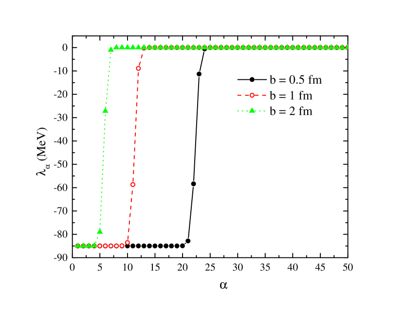
Figure 1: Eigenvalues $\lambda_{\alpha}$ of the square well potential energy operator versus the eigenvalue number $\alpha$ for three values of oscillator length $b=0.5$ fm, $b=1$ fm and $b=2$ fm.

However, it is a superficial difference. If we plot the eigenvalues $\lambda_{\alpha}$ against a discrete coordinate $r_{\alpha}^{N}$ (see Fig. 2), we will find that the depth and the range of the square well potential in the representation of its eigenvalues are the same for all the values of the oscillator length and coincide with those of the original potential. The only difference is that the smaller is the oscillator length, the smaller is the increment of a discrete variable $r_{\alpha}^{N}$.

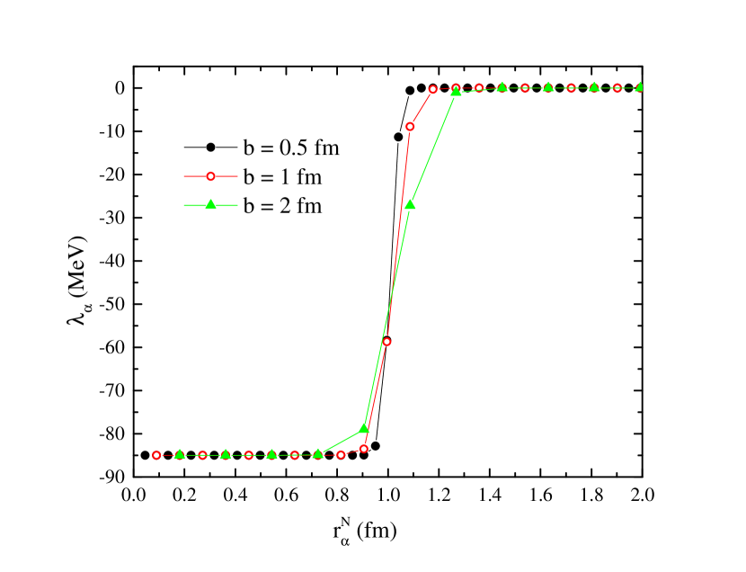
Figure 2: Eigenvalues $\lambda_{\alpha}$ of the square well potential energy operator versus a discrete coordinate $r_{\alpha}^{N}$ for three values of oscillator length $b=0.5$ fm, $b=1$ fm and $b=2$ fm.

Important information can be deduced from Fig. 1. We see that the large number of eigenvalues equal zero. The number of nonzero eigenvalues strongly depends on the oscillator length $b$. The smaller is $b$, the larger is the number of the eigenvalues $\lambda_{\alpha}\neq 0$. For all three values of $b$, the number of the non-vanishing eigenvalues is not more than 10% of the total number of the obtained eigenvalues. Thus, we can conclude that the real number of eigenvalues involved in Eqs. (45) and (2.4) to form wave function and T-matrix is very small. Similar situation is observed for other potentials. Due to relatively long tails of these potentials compared with the square-well potential, the number of the nonzero eigenvalues is larger, however the number of eigenvalues $\lambda_{\alpha}=0$ is even greater.

Fig. 3 shows perfect coincidence of the potential energy $V(r_{\alpha}^{N})$ in discrete points $r_{\alpha}^{N}$ with eigenvalues $\lambda_{\alpha}$ for the oscillator length $b=0.5$ fm, which is a half the range of the potential.

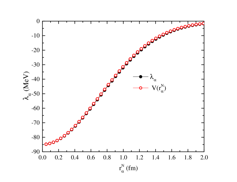
Figure 3: Eigenvalues $\lambda_{\alpha}$ of the Gaussian potential energy operator versus a discrete coordinate $r_{\alpha}^{N}$ for oscillator length $b=0.5$ fm. Potential energy $V(r_{\alpha}^{N})$ in discrete points is given by solid circles.

Fig. 4 demonstrates that small values of oscillator length scan the potential in more detail.

Figure 4: Eigenvalues $\lambda_{\alpha}$ of the Gaussian potential energy operator versus a discrete coordinate $r_{\alpha}^{N}$ for three values of oscillator length $b=0.5$ fm, $b=1$ fm and $b=2$ fm.

Fig. 5 and Fig. 6 evidence that our conclusions are valid equally well for a Gaussian potential.

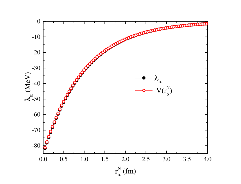
Figure 5: Eigenvalues $\lambda_{\alpha}$ of the exponential potential energy operator versus a discrete coordinate $r_{\alpha}^{N}$ for oscillator length $b=0.5$ fm. Potential energy $V(r_{\alpha}^{N})$ in discrete points is given by solid circles.

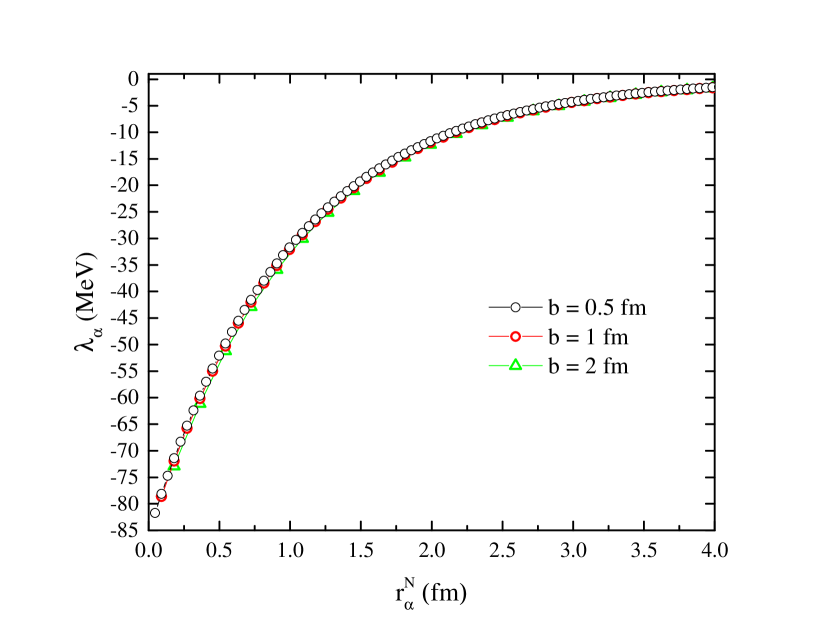
Figure 6: Eigenvalues $\lambda_{\alpha}$ of the exponential potential energy operator versus a discrete coordinate $r_{\alpha}^{N}$ for three values of oscillator length $b=0.5$ fm, $b=1$ fm and $b=2$ fm.

Figure 7 represents the dependence of the eigenvalues of the Yukawa potential energy operator on the eigenvalue number and oscillator length. We have chosen this potential to check how the shape of a singular at zero potential is reproduced by its eigenvalues $\lambda_{\alpha}$. As can be observed from Fig. 7, quite small values of oscillator length are needed to reach an interior part of the potential.

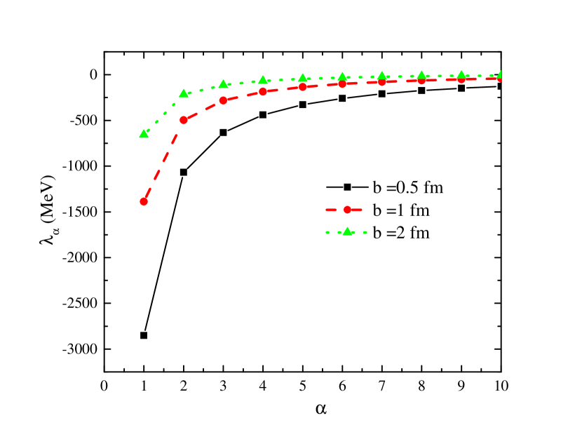
Figure 7: Eigenvalues $\lambda_{\alpha}$ of the Yukawa potential energy operator versus a number of eigenvalue $\alpha$ for three values of oscillator length $b=0.5$ fm, $b=1$ fm and $b=2$ fm.

Fig. 8 demonstrates that Yukawa potential is also well reproduced by the behavior of its eigenvalues, although the coincidence with the original potential at very small values of a discrete variable is not so ideal as for a non-singular potential.

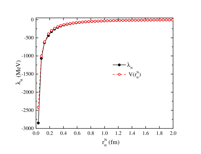
Figure 8: Eigenvalues $\lambda_{\alpha}$ of the Yukawa potential energy operator versus a discrete coordinate $r_{\alpha}^{N}$ for oscillator length $b=0.5$ fm. Potential energy $V(r_{\alpha}^{N})$ in discrete points is given by solid circles.

At the same time, Fig. 9 demonstrates the same regularity as the other potentials, namely, the more detailed scanning of the shape of the potential by smaller values of oscillator length.

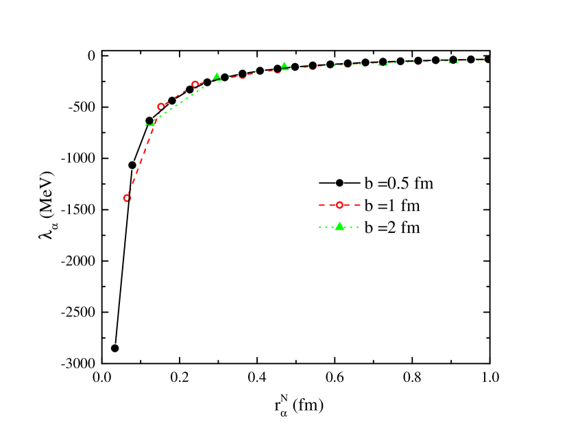
Figure 9: Eigenvalues $\lambda_{\alpha}$ of the Yukawa potential energy operator versus a discrete coordinate $r_{\alpha}^{N}$ for three values of oscillator length $b=0.5$ fm, $b=1$ fm and $b=2$ fm.

Eigenfunctions $U^{\alpha}_{n}$ of the Yukawa potential energy operator in the harmonic oscillator representation corresponding to the three lowest eigenvalues $\lambda_{\alpha},$ $\alpha=1,2,3$ are plotted against the number of oscillator quanta $n$ in Figs.10, 11, 12. Oscillator length $b$ was chosen to be equal to the range of the potential.

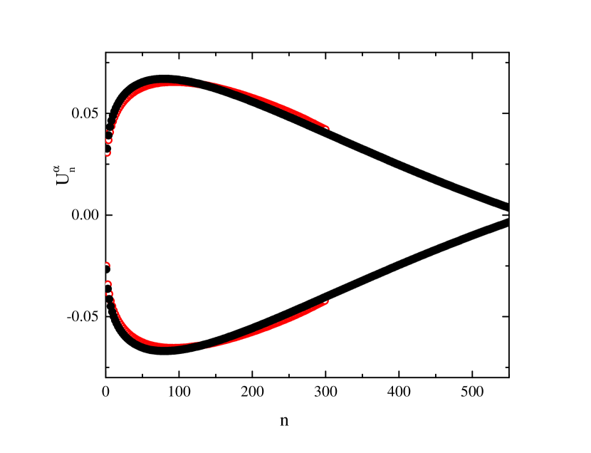
Figure 10: Eigenfunction $U^{\alpha}_{n},$ $\alpha=1$ of the Yukawa potential energy operator in the discrete representation versus the number of oscillator quanta $n$ for oscillator length $b=1$ fm. Extrapolated eigenfunction (Oscillator function $\mathcal{N}_{\alpha}\Phi_{n}(r^{N}_{\alpha},b)$) is given by solid circles.

In Figs.10, 11, 12 we can observe that eigenfunctions $U^{\alpha}_{n}$ are oscillator functions $\Phi_{n}(r^{N}_{\alpha},b)$, as was concluded in the previous Section of the paper. Predictably, in the range from zero to $N_{max}$ eigenfunction $U^{\alpha=1}_{n}$ is nodeless, while $U^{\alpha=2}_{n}$ has a node, and $U^{\alpha=3}_{n}$ has two nodes.

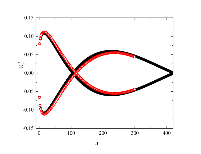
Figure 11: Eigenfunction $U^{\alpha}_{n},$ $\alpha=2$ of the Yukawa potential energy operator in the discrete representation versus the number of oscillator quanta $n$ for oscillator length $b=1$ fm. Extrapolated eigenfunction (Oscillator function $\mathcal{N}_{\alpha}\Phi_{n}(r^{N}_{\alpha},b)$) is given by solid circles.

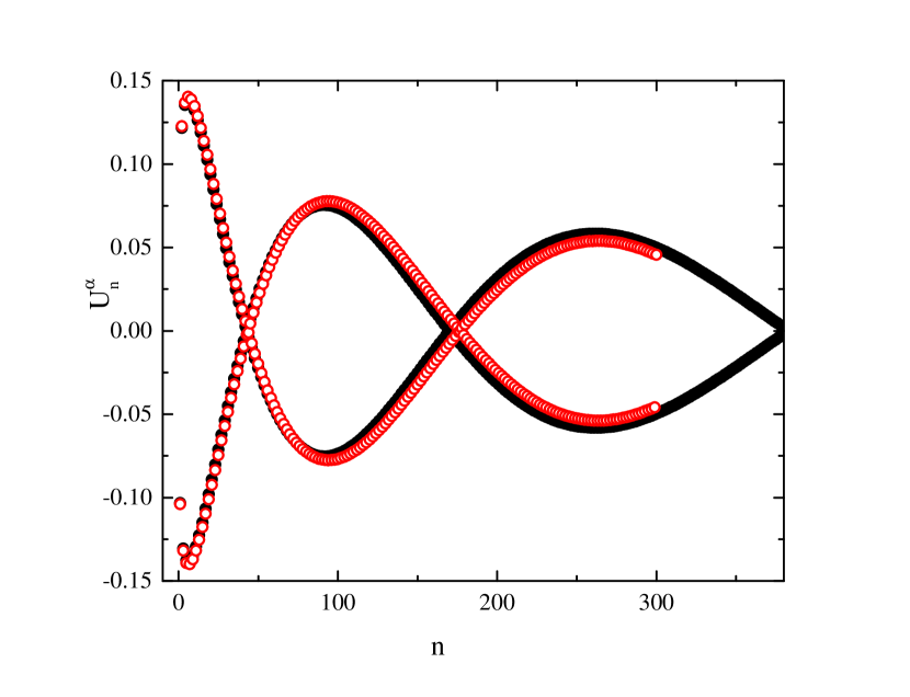
Figure 12: Eigenfunction $U^{\alpha}_{n},$ $\alpha=3$ of the Yukawa potential energy operator in the discrete representation versus the number of oscillator quanta $n$ for oscillator length $b=1$ fm. Extrapolated eigenfunction (Oscillator function $\mathcal{N}_{\alpha}\Phi_{n}(r^{N}_{\alpha},b)$) is given by solid circles.

Figures 13 and 14 present eigenfunctions $U^{\alpha}_{n},$ $\alpha=1,2$ for a Gaussian, an exponential, and Yukawa potentials. In all the cases the oscillator length is equal to the range of the potential. Figures 13, 14 demonstrate close resemblance of the eigenfunctions which proves their universality. Indeed, all the eigenfunctions are the harmonic oscillator functions corresponding to the same value of the oscillator length. The difference between the eigenfunctions for different potentials is due to the distinction between the corresponding discrete coordinates $r^{N}_{\alpha}.$ In turn, value of $r^{N}_{\alpha}$ is determined by the location of the $\alpha$th node of the eigenfunction, i.e., the number of oscillator quanta $N$.

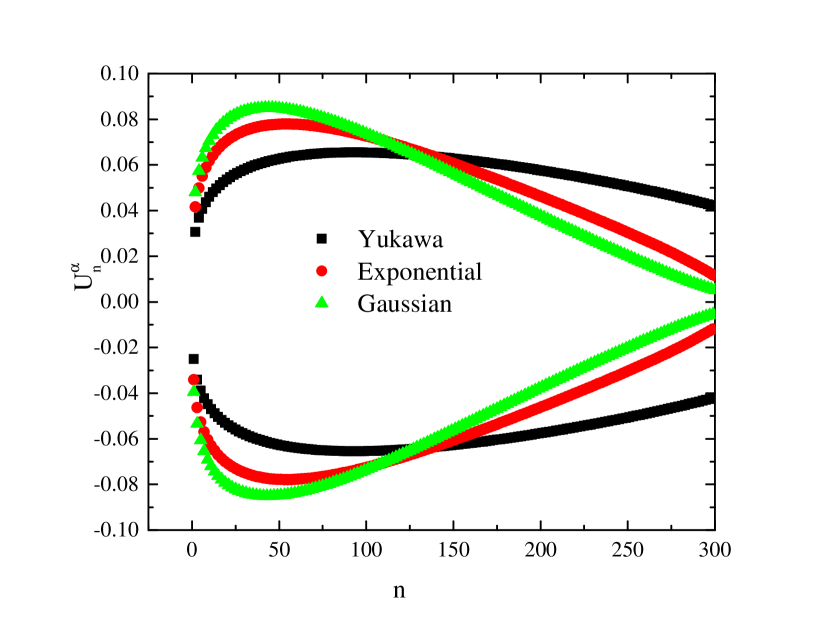
Figure 13: Eigenfunctions $U^{\alpha}_{n},$ $\alpha=1$ of the potential energy operator for different potentials in the discrete representation versus the number of oscillator quanta $n$ for oscillator length $b=1$ fm. The types of the potentials are shown in the figure.

As can be observed from Fig. 13, the eigenfunction of the Yukawa potential has the first node much farther than the eigenfunctions of two other potentials. That is why the distinction between the eigenfunctions of a Gaussian and an exponential potential is less than the difference between the latter eigenfunctions and the eigenfunction of the Yukawa potential.

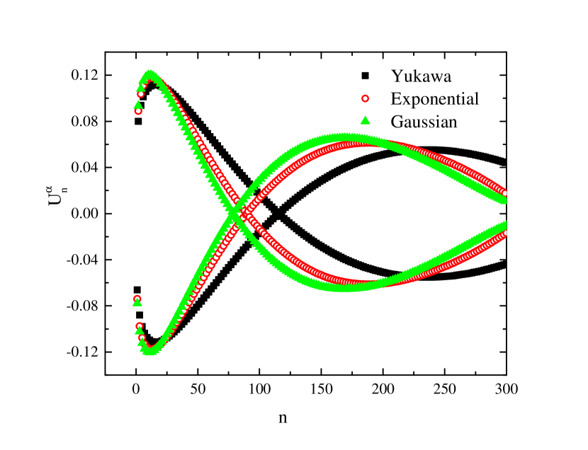
Figure 14: Eigenfunctions $U^{\alpha}_{n},$ $\alpha=2$ of the potential energy operator for different potentials in the discrete representation versus the number of oscillator quanta $n$ for oscillator length $b=1$ fm. The types of the potentials are shown in the figure.

3.0.3 Comparison

There is another way to demonstrate the validity of the expression (33) for the eigenfunctions of the potential energy matrix in the oscillator representation. Suppose we obtained eigenfunctions and eigenvalues of the same potential with two different numbers of oscillator functions $N_{1}$ and $N_{2}$, with $N_{1}<N_{2}$. And suppose that the eigenvalue $\lambda_{\alpha_{1}}$ obtained with $N_{1}$ oscillator functions approximately equals the eigenvalue $\lambda_{\alpha_{2}}$ calculated with $N_{2}$ oscillator functions. Then the eigenfunctions $U_{n}^{\alpha_{1}}$ and $U_{n}^{\alpha_{2}}$ will have the similar behavior in the common range of $n$: $0\leq n\leq N_{1}-1$. They have approximately the same value of $r_{\alpha}$, but differ in the normalization constants $\mathcal{N}_{\alpha_{1}}$and $\mathcal{N}_{\alpha_{2}}$. If the eigenfunctions $U_{n}^{\alpha_{1}}$ have one or more nodes in the range $0\leq n\leq N_{1}-1$, the eigenfunction $U_{n}^{\alpha_{2}}$ should have node(s) at the same point(s). By using a common normalization constant, for example $\mathcal{N}_{\alpha_{1}}$, for both eigenfunctions $U_{n}^{\alpha_{1}}$ and $U_{n}^{\alpha_{2}}$, we will see that they totally coincide in the range $0\leq n\leq N_{1}-1$.

This statement is demonstrated in Fig. 15 for the exponential potential. These results are obtained with the oscillator length $b$= 1 fm. Two eigenfunctions displayed in Fig. 15 are obtained with $N_{1}$=163 and $N_{2}$=300 oscillator functions. We compare eigenfunctions for the $\alpha_{1}=3$ and $\alpha_{2}=4$ eigenstates which have very close eigenvalues $\lambda_{\alpha_{1}}\approx\lambda_{\alpha_{2}}$. As we see, these two eigenfunctions have a similar behavior in the range $0\leq n\leq 162$, and besides they have two nodes at the same value of $n$. We do not renormalize them in the same fashion, thus they slightly differ.

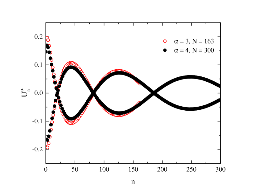
Figure 15: Eigenfunctions of the potential energy matrix in the oscillator representation obtained for the exponential potential with $b$=1 fm and two different numbers of the oscillator functions.

Fig. 16 and Fig. 17 depict first three eigenfunctions $\phi_{\alpha}(r)$ of the Gaussian and Yukawa potentials in coordinate representation. We can observe that the smaller is the eigenvalue number $\alpha$, the more the corresponding eigenfunction resembles the delta function. It might be well to point out that the number of nodes in the eigenfunctions increases with increasing the eigenvalue number $\alpha.$

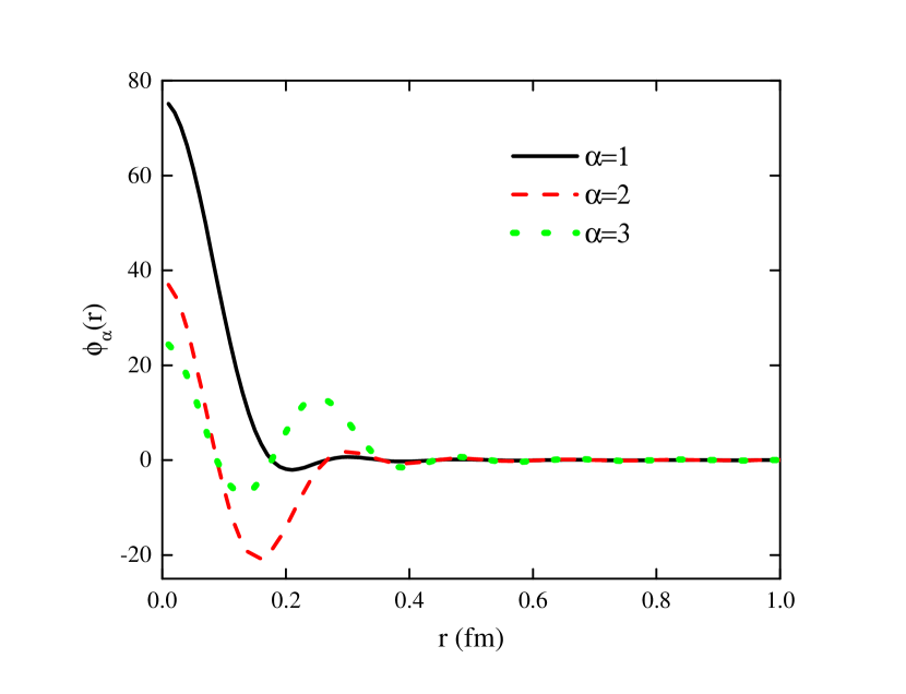
Figure 16: Eigenfunctions $\phi_{\alpha}(r)$ of the Gaussian potential energy operator in the coordinate representation for oscillator length $b=1$ fm. Values of $\alpha$ are indicated in the figure.

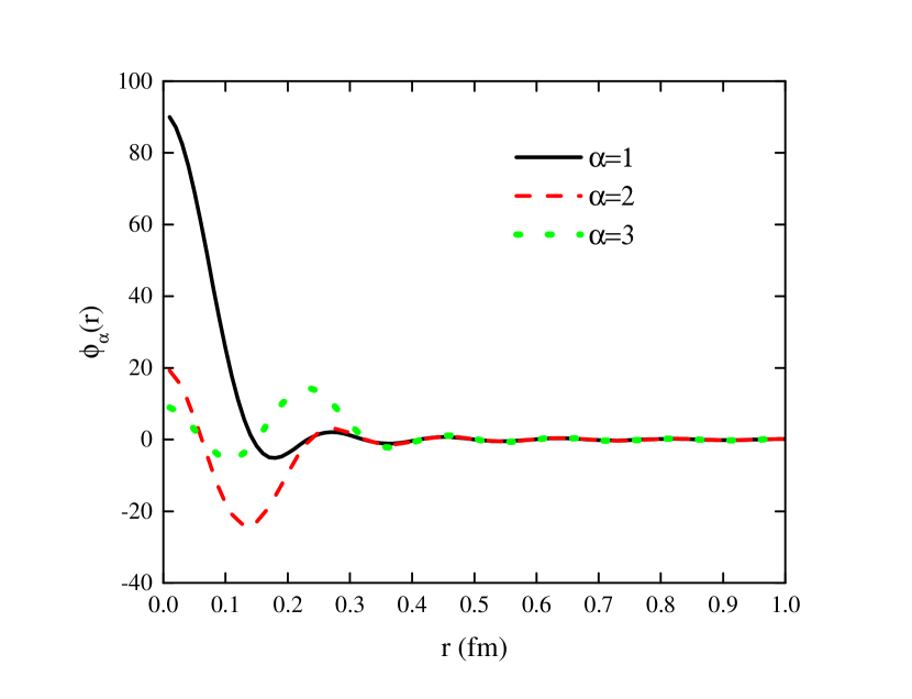
Figure 17: Eigenfunctions $\phi_{\alpha}(r)$ of the Yukawa potential energy operator in the coordinate representation for oscillator length $b=1$ fm. Values of $\alpha$ are indicated in the figure.

Fig. 18 and Fig. 19 display eigenfunctions $\phi_{\alpha}(p)$ of the Gaussian and Yukawa potential energy operator in the momentum representation. The figures support our conclusion that eigenfunctions $\phi_{\alpha}(p)$ are simply Bessel functions $j_{0}(pr_{\alpha}^{N})$. Since the discrete coordinate $r_{\alpha}^{N}$ increases with $\alpha,$ the corresponding eigenfunction $\phi_{\alpha}(p)$ exhibits more oscillations with increase in $\alpha.$ Eigenfunctions of the Gaussian and Yukawa potential energy operators are very similar, because $r_{\alpha}^{N}$ depends only slightly on the location of the $\alpha$th zero of the eigenfunction $U^{\alpha}_{n}$ in the discrete representation.

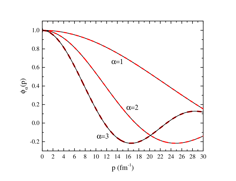
Figure 18: Eigenfunctions $\phi_{\alpha}(p)$ (solid lines) of the Gaussian potential energy operator in the momentum representation for oscillator length $b=1$ fm and Bessel functions $j_{0}(pr_{\alpha})$ (dashed lines). Values of $\alpha$ are indicated near the curves.

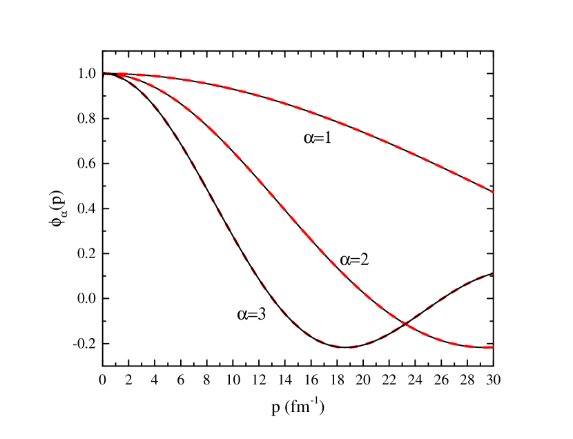
Figure 19: Eigenfunctions $\phi_{\alpha}(p)$ (solid lines) of the Yukawa potential energy operator in the momentum representation for oscillator length $b=1$ fm and Bessel functions $j_{0}(pr_{\alpha})$ (dashed lines). Values of $\alpha$ are indicated near the curves.

3.0.4 Wave function of square-well potential.

As one may notice, we do not show the eigenfunctions of the square-well potential. They have a rather complicated form and may confuse the reader of the present paper. The complexity originates from the degenerate states. Indeed, in this case we have many degenerate eigenvalues which coincide with the depth of the square-well potential. Numerical diagonalization procedure reveals such eigenfunctions which are a specific orthogonal combination of the correct (canonical) eigenfunctions presented by Eq. (33). One may try to decompose the nonstandard eigenfunctions in a set of standard ones. We do not perform such a decomposition as it involves painstaking efforts and does not supply us with new information.

In this respect it is important to notice that any potential, which contains the repulsive and attractive parts, will or may have the twofold degenerate eigenvalues, one of which corresponds to a repulsive part and the other corresponds to an attractive part of the potential. And thus their eigenfunctions will be of a complicated unusual form. It is then necessary to study what combinations of the standard eigenfunctions are presented in the obtained eigenfunctions.

4 Conclusions

We have studied the main properties of the potential energy matrix for a model problem - particle in a field of central-symmetric potential. We have selected four types of potentials which are very often used both for model and real physical problems. They are square-well, Gaussian, exponential and Yukawa potentials. We have obtained and analyzed the structure of eigenvalues and eigenfunctions of the potential energy matrix in a huge but finite basis of oscillator functions. We demonstrated that eigenvalues of the matrix coincide with the potential energy in some specific points of the coordinate space, and eigenfunctions are the expansion coefficients of the spherical Bessel functions over oscillator functions. These are the universal properties of matrix elements of two-body potential matrix.

We have demonstrated that the large part of eigenvalues of the potentials equals zero. It means that only a very restricted number of the potential eigenstates participates in the wave function of scattering state and T-matrix. The dependence of the eigenvalues on the shape of potentials and oscillator length explains why and when we need a small number of basis functions to obtain wave functions and scattering parameters with the desired precision.

We have used an oscillator basis to construct matrix elements of the potential energy operator and to study its eigenvalues and eigenfunctions. However, the eigenfunctions of the potential in the discrete representation will be the expansion coefficients of the spherical Bessel function for any square-integrable orthonormal basis, while the eigenvalues of the potential will be determined by a location of the zeros of these eigenfunctions. The only difference will be in the explicit form of the eigenfunctions of the potential.

The results of the analysis of eigenvalues and eigenfunctions of the potential energy matrix performed in the present paper for model potentials will be used to study properties of the potential energy operator for real physical problems, namely, for a set of atomic nuclei which can be presented as a two-cluster system.

By comparing eigenvalues and eigenfunctions of the potential energy operator obtained with and without (the so-called folding approximation) total antisymmetrization, we are going to reveal effects of the Pauli principle in nuclear two-cluster systems.

As we seen above, the diagonalization of the potential energy matrix proposes a self consistent way of reducing a nonlocal potential (or nonlocal operator) to the local form. It is intriguing to study what local form could suggest this method for two-cluster systems. That will be a subject of the next paper.

After publication of the present paper on the site of electronic preprints, we were informed about the papers [37, 38] where the approximate formula is used to calculate matrix elements of different two-body potentials. This formula is similar to the expression (29) we have deduced. In Refs. [37, 38] the approximate method is based on the theorems for the numerical calculations of integrals involving orthogonal polynomials. Such theorems can be found in the book [23]. To calculate matrix elements of the potential energy operator, we have not used this approximate method. As pointed out above, we have used the recurrence relations. Our results demonstrate that the effective size of the matrix $\left\|U_{n}^{\alpha}\right\|$ in Eq. (29) (i.e. the position of a remote node determined in section (3.0.1)) depends on the potential shape and the oscillator length $b$. By comparing our results with the approximate formula used in Refs. [37, 38], we came to the conclusion that the approximate method is very precise for relatively small values of the oscillator length $b$ and for potentials without singularity.

References

- [1] E. J. Heller, H. A. Yamani, New approach to quantum scattering: Theory, Phys. Rev. A9 (1974) 1201–1208. doi:10.1103/PhysRevA.9.1201.
- [2] H. A. Yamani, L. Fishman, -matrix method: Extensions to arbitrary angular momentum and to Coulomb scattering, J. Math. Phys. 16 (1975) 410–420. doi:10.1063/1.522516.
- [3] G. F. Filippov, I. P. Okhrimenko, Use of an oscillator basis for solving continuum problems, Sov. J. Nucl. Phys. 32 (1981) 480–484.
- [4] G. F. Filippov, On taking into account correct asymptotic behavior in oscillator-basis expansions, Sov. J. Nucl. Phys. 33 (1981) 488–489.
- [5] A. D. Alhaidari, H. A. Yamani, E. J. Heller, M. S. Abdelmonem (Eds.), The -Matrix Method. Developments and Applications, Springer, Netherlands, 2008.
- [6] A. M. Lane, R. G. Thomas, R-Matrix Theory of Nuclear Reactions, Rev. Mod. Phys. 30 (2) (1958) 257–353. doi:10.1103/RevModPhys.30.257.
- [7] Z. Papp, Three-potential formalism for the three-body Coulomb scattering problem, Phys. Rev. C 55 (1997) 1080–1087. arXiv:nucl-th/9701027, doi:10.1103/PhysRevC.55.1080.
- [8] P. Doleschall, Z. Papp, p-d scattering with a nonlocal nucleon-nucleon potential below the breakup threshold, Phys. Rev. C 72 (4) (2005) 044003. doi:10.1103/PhysRevC.72.044003.
- [9] Y. V. Popov, S. A. Zaytsev, S. I. Vinitsky, J-matrix method for calculations of three-body Coulomb wave functions and cross sections of physical processes, Phys. Part. Nucl. 42 (5) (2011) 683–712. doi:10.1134/S1063779611050042.
- [10] S. Keller, A. Marotta, Z. Papp, Faddeev-Merkuriev integral equations for atomic three-body resonances, J. Phys. B At. Mol. Phys. 42 (4) (2009) 044003. arXiv:0810.3036, doi:10.1088/0953-4075/42/4/044003.
- [11] I. Okhrimenko, Allowance for the Coulomb interaction in the framework of an algebraic version of the resonating group method, Nucl. Phys. A424 (1984) 121–142.
- [12] T. Y. Mikhelashvili, A. M. Shirokov, Y. F. Smirnov, Monopole excitations of the 12C nucleus in the cluster model, J. Phys. G Nucl. Phys. 16 (1990) 1241–1251. doi:10.1088/0954-3899/16/8/020.
- [13] Y. A. Lurie, A. M. Shirokov, Loosely bound three-body nuclear systems in the J-matrix approach, Ann. Phys. 312 (2004) 284–318. arXiv:arXiv:nucl-th/0312028, doi:10.1016/j.aop.2004.02.002.
- [14] A. V. Nesterov, F. Arickx, J. Broeckhove, V. S. Vasilevsky, Three-cluster description of properties of light neutron- and proton-rich nuclei in the framework of the algebraic version of the resonating group method, Phys. Part. Nucl. 41 (5) (2010) 716–765. doi:10.1134/S1063779610050047.
- [15] P. Descouvemont, D. Baye, The R-matrix theory, Rep. Prog. Phys. 73 (3) (2010) 036301. arXiv:1001.0678, doi:10.1088/0034-4885/73/3/036301.
- [16] D. Baye, P.-H. Heenen, M. Libert-Heinemann, Microscopic R-matrix theory in a generator coordinate basis (III). Multi-channel scattering, Nucl. Phys. A 291 (1977) 230–240. doi:10.1016/0375-9474(77)90208-1.
- [17] P. Descouvemont, M. Dufour, Microscopic Cluster Models, Vol. 2, 2012, p. 1. doi:10.1007/978-3-642-24707-11.
- [18] D. Baye, The Lagrange-mesh method, Phys. Rep. 565 (2015) 1–107. doi:10.1016/j.physrep.2014.11.006.
- [19] Ismail, M. E. H. and Koelink, E., The J-matrix method, Advances in Applied Mathematics 46 (1) (2011) 379 – 395, special issue in honor of Dennis Stanton. doi:https://doi.org/10.1016/j.aam.2010.10.005.
- [20] M. E. H. Ismail, E. Koelink, Spectral Analysis of Certain Schrödinger Operators, SIGMA 8 (2012) 061. arXiv:1205.0821, doi:10.3842/SIGMA.2012.061.
- [21] M. E. H. Ismail, E. Koelink, Spectral properties of operators using tridiagonalization, Analysis and Applications, 10 (03) (2012) 327–343. arXiv:https://doi.org/10.1142/S0219530512500157, doi:10.1142/S0219530512500157.
- [22] M. Abramowitz, A. Stegun, Handbook of Mathematical Functions, Dover Publications, Inc., New-York, 1972.
- [23] V. I. Krylov, Approximate calculation of integrals, MacMillan, New York, 1962.
- [24] F. Gantmacher, The theory of matrices, Chelsea Publ. Company, New York, 1960.
- [25] Y. A. Lashko, G. F. Filippov, V. S. Vasilevsky, Dynamics of two-cluster systems in phase space, Nucl. Phys. A 941 (2015) 121–144. arXiv:1503.06005, doi:10.1016/j.nuclphysa.2015.06.006.
- [26] V. S. Vasilevsky, Y. A. Lashko, G. F. Filippov, Two- and three-cluster decays of light nuclei within a hyperspherical harmonics approach, Phys. Rev. C 97 (6) (2018) 064605. doi:10.1103/PhysRevC.97.064605.
- [27] R. G. Newton, Scattering Theory of Waves and Particles, McGraw-Hill, New-York, 1966.
- [28] V. B. Belyaev, Lectures on the Theory of Few-Body Syst., Springer-Verlag, LLC, New York, 1990.
- [29] A. L. Zubarev, Separable representation method in problems of nuclear physics, Sov. J. Part. Nucl. 7 (2) (1976) 215–227.
- [30] A.I. Baz and Ya.B. Zel’dovich and A.M. Perelomov, Scattering, Reaction in Non-Relativistic Quantum Mechanics., Israel Program for Scientific Translations, Jerusalem, 1969.
- [31] E. J. Heller, Theory of J-matrix Green’s functions with applications to atomic polarizability and phase-shift error bounds, Phys. Rev. A 12 (1975) 1222–1231.
- [32] F. Arickx, J. Broeckhove, P. van Leuven, V. Vasilevsky, G. Filippov, Algebraic method for the quantum theory of scattering, Amer. J. Phys. 62 (1994) 362–370.
- [33] V. S. Vasilevsky, F. Arickx, Algebraic model for quantum scattering: Reformulation, analysis, and numerical strategies, Phys. Rev. A55 (1997) 265–286.
- [34] J. Broeckhove, V. Vasilevsky, F. Arickx, A. Sytcheva, On the Regularisation in J-matrix Methods, ArXiv Nuclear Theory e-prints nucl-th/0412085.
- [35] J. Broeckhove, V. S. Vasilevsky, F. Arickx, A. M. Sytcheva, On the Regularization in -Matrix Methods, in: A. D. Alhaidari, H. A. Yamani, E. J. Heller, M. S. Abdelmonem (Eds.), The -Matrix Method. Developments and Applications, Springer, Netherlands, 2008, pp. 117–134.
- [36] V. S. Vasilevsky, M. D. Soloha-Klymchak, T-matrix in discrete oscillator representation, Ukr. J. Phys. 60 (4) (2015) 297–306.
- [37] A. D. Alhaidari, H. A. Yamani, M. S. Abdelmonem, Relativistic J-matrix theory of scattering, Phys. Rev. A 63 (6) (2001) 062708. doi:10.1103/PhysRevA.63.062708.
- [38] I. Nasser, M. S. Abdelmonem, H. Bahlouli, A. D. Alhaidari, The rotating Morse potential model for diatomic molecules in the tridiagonal J-matrix representation: I. Bound states, J. Phys. B At. Mol. Phys. 40 (21) (2007) 4245–4257. arXiv:0706.2371, doi:10.1088/0953-4075/40/21/011.