Spectroscopic study on hot-electron transport in a quantum Hall edge channel

Abstract

Hot electron transport in a quantum Hall edge channel of an AlGaAs/GaAs heterostructure is studied by investigating the energy distribution function in the channel. Ballistic hot-electron transport, its optical-phonon replicas, weak electron-electron scattering, and electron-hole excitation in the Fermi sea are clearly identified in the energy spectra. The optical-phonon scattering is analyzed to evaluate the edge potential profile. We find that the electron-electron scattering is significantly suppressed with increasing the hot-electron’s energy well above the Fermi energy. This can be understood with suppressed Coulomb potential with longer distance for higher energy. The results suggest that the relaxation can be suppressed further by softening the edge potential. This is essential for studying non-interacting chiral transport over a long distance.

I Introduction

Hot electrons with the energy greater than the Fermi energy are subject to relaxation processes such as electron-electron and electron-phonon scattering BookRidley ; EE2D-Giuliani ; EE2D-negativeR ; EE1D-Karzig ; EP2D-Sivan ; EPlowD-Bockelmann . Therefore, ballistic and coherent electron transport is usually expected only at low temperatures and low-energy excitation BookNazarov ; hotEB=0-Rossler . This also applies to chiral edge channels in the integer quantum Hall regime QHMZ-YJi ; QHHOM-Freulon ; QHMZee-Tewari . While the conductance is quantized due to the absence of backscattering, forward scattering is so significant that electronic excitation easily relaxes to collective excitations in the plasmon modes leSueurPRL2010 ; HashisakaNatPhys . This relaxation length is only a few $\mu$m when a small excitation energy of about 30 $\mu$eV is used for a GaAs heterostructure, and decreases with increasing energy in agreement with the spin-charge separation in the Tomonaga-Luttinger model leSueurPRL2010 ; TwoStage-Itoh . However, recent experiments using a depleted edge HotEDyQD-Kataoka or a high-magnetic field HotEDyQD-Fletcher ; HotEDyQD-Ubbelohde have demonstrated ballistic transport over 1 mm for hot electrons with surprisingly large energy of about 100 meV above the Fermi energy HotEDyQD-Johnson . In this high-energy region greater than the optical phonon energy, the optical-phonon scattering process has been studied extensively. The relaxation in the intermediate energy region is yet to be investigated for how the electron-electron scattering has been suppressed. This is particularly important for realizing coherent transport of hot electrons QHMZee-Tewari ; HotE-coherence-STM , as the coherency can be reduced with the electron-electron scattering if exists. For the experiments on quantum Hall edges, most of the works were devoted to study low energy excitation below 1 meV. Taubert et al. have investigated electron-hole excitation in the Fermi sea, from which some hydrodynamic effects as well as optical-phonon scattering are studied for higher energy greater than 100 meV HotE-TaubertB=0 ; HotE-TaubertB>0 ; HotE-Taubert . However, this non-spectroscopic scheme is not convenient for the purpose. High-energy hot electron can be excited with a dynamic quantum dot driven by high-frequency voltage. This scheme is attractive for generating a single hot electron, but not convenient for tuning the energy in the wide range of interest. Systematic measurements with a spectroscopic scheme are highly desirable to investigate the hot-electron transport.

In this work, hot-electron spectroscopy is employed, where hot electrons are injected from a point contact (PC) to an edge channel and the electrons after propagation are investigated by using an energy spectrometer made of a similar PC. With fine tuning of gate voltages on injector and detector PCs, we have investigated ballistic hot-electron transport, multiple emission of optical phonons showing ‘phonon replicas’, small energy reduction associated with weak electron-electron scattering, and electron-hole plasma in the Fermi sea. They are explained with electron-electron scattering and electron-phonon scattering, which can be tuned with the soft edge potential. This electric-field effect will be useful in designing one-dimensional hot-electron circuits.

II Measurement scheme

Consider a two-dimensional electron system (2DES) under a perpendicular magnetic field $B$ in the $-z$ direction (to the back of the 2DES). Near the edge of the 2DES, Landau levels increase with the soft edge potential along $x$ axis as illustrated in Fig. 1(a) for the lowest Landau levels (LLLs) with spin up and down branches. Here, Landau-level filling factor $\nu$ in the range of $1<\nu<2$ is considered as a simplest case to study. This energy profile can be regarded as the energy - momentum ($k_{y}=eBx/\hbar$) dispersion relation under the Landau gauge BookEzawa . We focus on hot spin-up electrons well above the chemical potential $\mu$.

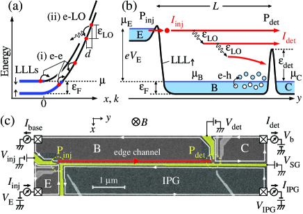
Figure 1: (a) Schematic energy diagram of the lowest Landau levels (LLLs) for spin-up an -down electrons. Electron-electron scattering (i) and LO phonon scattering (ii) are illustrated. (b) Schematic energy diagram of hot electron spectroscopy. A hot electron injected from emitter E experiences relaxation associated with LO phonon emission and electron-electron scattering. Resulting energy distribution function is measured with tunable barrier $\varepsilon_{\det}$. (c) The measurement setup with a scanning electron micrograph of a $L=$ 5 $\mu$m device. Other devices have slightly different gate patterns but conceptually the same. Bias voltage $-V_{\mathrm{E}}$ (with positive $V_{\mathrm{E}}$) is applied on the emitter contact to inject hot electrons to the edge channel.

The dominant relaxation processes in this system are also illustrated in Fig. 1(a). Diagram (i) shows the electron-electron scattering between the hot spin-up electron and cold electrons near the chemical potential LundePRB2010-EE ; LundePRB-EE . As the potential profile and thus the dispersion is nonlinear, the two-particle scattering for exchanging equal energy is basically forbidden as it cannot conserve the total momentum. The scattering is practically allowed in the presence of random impurity potential that breaks the translational invariance along $y$ axis. The electron-electron scattering would be less probable for hotter electrons with two reasons, as larger momentum mismatch and larger spatial separation are involved. We investigate these effects in our experiment.

Diagram (ii) shows the optical-phonon scattering, where electron loses its energy by emitting a longitudinal optical (LO) phonon with energy $\varepsilon_{\mathrm{LO}}=$ 36 meV in GaAs HotEDyQD-Kataoka . This phonon emission is suppressed by large spatial shift $d$ in the guiding center of the electron motion, when $d$ is greater than the magnetic length $\ell_{\mathrm{B}}=\sqrt{\hbar/eB}$. We use this characteristics to evaluate the effective electric field (or the potential profile) of the channel. This provides better understanding of electron-electron scattering as well as optical phonon scattering.

Figure 1(b) illustrates the measurement scheme for the hot electron spectroscopy. The thick solid line labeled LLL_↑ shows the spin-up LLL (mostly in the bulk region) along the transport direction ($y$ axis). The injector PC labeled $\mathrm{P}_{\mathrm{inj}}$ and the detector PC labelled P_det separate three conductive regions; the emitter (labeled E), the base (B), and the collector (C). These regions are filled with electrons up to the respective chemical potentials, $\mu_{\mathrm{E}}$, $\mu_{\mathrm{B}}$, and $\mu_{\mathrm{C}}$, at the edges of the conductive regions. With a large bias voltage $-V_{\mathrm{E}}$ on the emitter, hot electrons with energy $eV_{\mathrm{E}}$ ($=\mu_{\mathrm{E}}-\mu_{\mathrm{B}}$) are injected from the emitter to the edge channel in the base. Here, we assume that electrons are injected primarily into the spin-up LLL in the base region, as tunneling to the spin-down LLL as well as the second Landau levels (SLLs) is less probable with the thicker and higher barriers.

In the base region, the hot electron loses its energy step by step by emitting optical phonons and by generating electron-hole plasma in the Fermi sea via electron-electron scattering. The resulting energy distribution function is investigated with the detector P_det located at distance $L$ from $\mathrm{P}_{\mathrm{inj}}$. Electrons with the energy greater than barrier height $\varepsilon_{\det}$ are introduced to the collector ($\mu_{\mathrm{C}}\simeq 0$), while other electrons with lower energy are reflected and drained to the grounded based contact ($\mu_{\mathrm{B}}=0$). Therefore, the hot-electron spectroscopy can be performed by measuring current $I_{\det}$ through P_det at various $\varepsilon_{\det}$.

Our measurement setup in the quantum Hall regime is shown in Fig. 1(c) with a scanning electron micrograph of a test device. Surface metal gates (colored yellow) were patterned on a modulation doped GaAs/AlGaAs heterostructure (black). Magnetic field $B$ was applied perpendicular to the heterostructure to form edge channels, and most of the measurements were performed at bulk filling factor $\nu$ in the range of $1<\nu<2$. The main edge channel (the red line) in the base is formed along the side gate SG. The edge potential profile can be tuned with gate voltages $V_{\mathrm{SG}}$ on SG and $-V_{\mathrm{IPG}}$ on the other edge channel working as an in-plane gate (IPG). Particularly, $V_{\mathrm{IPG}}=$ 0 - 0.2 V, with the same sign of $V_{\mathrm{E}}$, is applied to eliminate the leakage of hot electrons to the IPG. Tunneling barriers of the injector ($\mathrm{P}_{\mathrm{inj}}$) and the detector (P_det) were adjusted by tuning voltages, $V_{\mathrm{inj}}$ and $V_{\mathrm{\det}}$, respectively. Several devices with different $L$ = 0.7, 1.4, 5, 8, 10 and 15 $\mu$m were formed with two-dimensional electron density $n_{\mathrm{2DES}}=$ 2.9$\times$10¹¹ cm^-2 (the zero-field Fermi energy of about 10 meV) and low-temperature mobility of $\mu_{\mathrm{2DES}}=$ 1.6$\times$10⁶ cm²/Vs (wafer W1) WashioPRB or $n_{\mathrm{2DES}}=$ 2.6$\times$10¹¹ cm^-2 and $\mu_{\mathrm{2DES}}=$ 3$\times$10⁶ cm²/Vs (wafer W2). All measurements were performed at 1.5 - 2.1 K.

III Hot-electron spectra

We measure the injection current $I_{\mathrm{inj}}$ and the detection current $I_{\mathrm{\det}}$, which are defined as positive for forward electron transport in the direction shown by the arrows in Fig. 1(c). Ammeters with a relatively large input impedance of $Z_{\mathrm{m}}=$ 10 k$\Omega$ - 1 M$\Omega$ were used to prevent possible damage with unwanted large current. The voltage drop in the ammeter is negligible for typical current level of 0.1 - 1 nA, while some influences on measuring the electron-hole plasma will be discussed later. The average number of injected electrons travelling in the channel of length $L$, $I_{\mathrm{inj}}L/ev_{\mathrm{h}}$, is kept less than one, where $v_{\mathrm{h}}=E/B$ is the hot-electron velocity for the electric field $E$ (discussed later) of the edge potential, and thus the interaction between the injected electrons can be neglected. The base current $I_{\mathrm{base}}$ at the base ohmic contact and the leakage current $I_{\mathrm{IPG}}$ at IPG were always monitored to ensure no leakage current ($I_{\mathrm{IPG}}=0$ and $I_{\mathrm{\det}}+I_{\mathrm{base}}=I_{\mathrm{inj}}$) within the noise level.

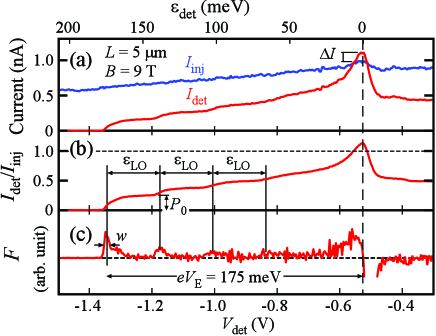
Figure 2: (a) $I_{\mathrm{\det}}$ and $I_{\mathrm{inj}}$, (b) $I_{\mathrm{\det}}/I_{\mathrm{inj}}$, and (c) $F=d(I_{\mathrm{\det}}/I_{\mathrm{inj}})/dV_{\mathrm{\det}}$ as a function of $V_{\mathrm{det}}$ for a $L=$ 5 $\mu$m device on wafer W1. The equispaced peaks in (c) represent the ballistic transport (the leftmost peak) and its phonon replicas. The step height $P_{0}$ in (b) measures the probability of ballistic transport for $L=$ 5 $\mu$m. The peak with $I_{\mathrm{\det}}/I_{\mathrm{inj}}>1$ in (b) shows electron-hole excitation in the Fermi sea, and thus defines the condition for $\varepsilon_{\det}=0$. The width $w$ (= 5 meV in energy) of the leftmost peak in (c) shows the energy resolution of this measurement.

Figure 2(a) shows a representative data of $I_{\mathrm{inj}}$ and $I_{\mathrm{\det}}$ at $V_{\mathrm{E}}=$ 175 mV as a function of $V_{\mathrm{\det}}$ for a $L$ = 5 $\mu$m device. As the injector P_inj with $I_{\mathrm{inj}}$ is slightly influenced by changing $V_{\mathrm{\det}}$, normalized current $I_{\mathrm{\det}}/I_{\mathrm{inj}}$ and its derivative $F=d(I_{\mathrm{\det}}/I_{\mathrm{inj}})/dV_{\mathrm{\det}}$ are evaluated as shown in Figs. 2(b) and 2(c), respectively. Here, $F$ is proportional to the energy distribution function of hot electrons in the edge channel. The periodic stepwise increase of $I_{\mathrm{\det}}$ (peaks in $F$) manifests multiple LO phonon emissions. The width of the peaks in $F$ is $w=$ 4 - 5 meV in energy, which is probably given by the energy dependent tunneling probability in $\mathrm{P}_{\mathrm{inj}}$ and $\mathrm{P}_{\mathrm{\det}}$. This determines the energy resolution of the spectroscopy. In the narrow region around $V_{\mathrm{\det}}\simeq-$0.55 V, the detector current exceeds the injection current ($I_{\mathrm{\det}}>I_{\mathrm{inj}}$), and the base current turns out to be negative ($I_{\mathrm{base}}<0$, not shown). This indicates electron-hole plasma in the base, where the electrons with energy above $\varepsilon_{\det}$ and the holes with energy below $\varepsilon_{\det}$ contribute excess detector current. Therefore, the peak position in $I_{\mathrm{\det}}$ determines the condition for $\varepsilon_{\mathrm{det}}=0$, where the top of the barrier in $\mathrm{P}_{\mathrm{\det}}$ is aligned to $\mu_{\mathrm{B}}$ ($\simeq\mu_{\mathrm{C}}$).

The energy scale of $\varepsilon_{\mathrm{det}}$ with respect to $V_{\mathrm{det}}$ is determined from the LO phonon replicas. For the data in Fig. 2(a), linear dependence $\Delta\varepsilon_{\mathrm{det}}=\alpha\Delta V_{\mathrm{det}}$ with the lever-arm factor $\alpha\simeq$ 0.213$e$ is confirmed from the equispaced LO phonon replicas. The spacing between the leftmost peak in $F$ for the ballistic transport ($\varepsilon_{\mathrm{det}}=eV_{\mathrm{E}}$) and the zero energy peak ($\varepsilon_{\mathrm{det}}=0$) in $I_{\mathrm{\det}}$ is consistent with this $\alpha$. While some devices showed nonlinearity in the $\varepsilon_{\mathrm{det}}$ - $V_{\mathrm{det}}$ relation, all spectroscopic analyses shown in this paper are made with reasonable linearity.

A color plot of $F$ in Fig. 3, taken with $L=$ 1.4 $\mu$m device, captures most of the features we discuss in this paper, where $V_{\mathrm{det}}$ is converted to $\varepsilon_{\mathrm{det}}$ shown in the right axis. In the high-energy region at $V_{\mathrm{E}}>$ 100 mV, the ballistic peak and its phonon replicas are clearly resolved along the dashed lines ($\varepsilon_{\mathrm{det}}=eV_{\mathrm{E}}-n\varepsilon_{\mathrm{LO}}$ with $n=$ 0, 1, and 2), which will be analyzed in Sec. IV. In the medium-energy region (30 mV $<V_{\mathrm{E}}<$ 60 meV), the highest-energy peak deviates from the ballistic condition ($\varepsilon_{\mathrm{det}}=eV_{\mathrm{E}}$), which will be explained with the weak electron-electron scattering in Sec. V. In the low-energy region ($V_{\mathrm{E}}<$ 30 meV), no ballistic signal is seen and the electron-hole excitation is clearly seen as a peak-and-dip structure near $\varepsilon_{\mathrm{det}}=0$. This electron-hole plasma is consistent with the weak electron-electron scattering as discussed in Sec. V. In this way, the hot-electron spectroscopy is informative for analyzing electron scattering.

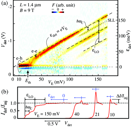
Figure 3: Representative hot-electron spectrum, $F$ as a function of $\varepsilon_{\det}$ on the right axis, for various $V_{E}$. The data is taken at $B$ = 9 T ($\nu=1.3$) with a $L=$ 1.4 $\mu$m device on wafer W2.

IV Optical-phonon scattering

First, we analyze the optical-phonon scattering showing the phonon replicas at $eV_{\mathrm{E}}>\varepsilon_{\mathrm{LO}}$ by ignoring the electron-electron scattering. As shown in the inset to Fig. 4(a), the hot electron in the LLL (the solid circle) can relax to a lower-energy state (the open circle) via two possible processes; direct LO (dLO) phonon emission within the LLL, and inter Landau level (iLL) tunneling to an intermediate state (the open square) in the SLL followed by inter-LL LO (iLO) phonon emission. Both can be dominant as studied in similar devices HotEDyQD-Johnson . In our spectroscopic measurement, occupation in the second Landau level (SLL) can be detected at a different condition, as the barrier height for the SLL, $\varepsilon_{\mathrm{det}}+\hbar\omega_{\mathrm{C}}$, is higher than $\varepsilon_{\mathrm{det}}$ for the LLL. A color-scale plot of $F$ in Fig. 4(a) shows such spectrum, where phonon replicas of hot electrons in LLL (along the horizontal solid lines) and SLL (along the dashed lines slanted by the cyclotron energy $\hbar\omega_{\mathrm{C}}$) are clearly seen. The peak spacing between the LLL and SLL phonon replicas increases linearly with $B$ in agreement with the cyclotron energy $\hbar\omega_{\mathrm{C}}$ [1.75 meV/T for GaAs]. This data shows coexistence of the two relaxation processes in this sample. The iLL tunneling may accompany acoustic phonon emission or absorption KomiyamaPRBspinflip , but the corresponding phonon energy is too small to be resolved in our measurement.

We find that this SLL signal appears only under some particular conditions in some particular devices. We did not see systematic dependencies on $L$ and $V_{\mathrm{E}}$. While further studies are required, this implies that the iLL tunneling is resonantly enhanced by an impurity or elsewhere. In contrast, the LLL phonon replicas associated with the dLO process are reproduced in various conditions. In the following, we analyze the LO phonon scattering for the data without showing SLL signals.

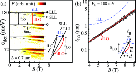
Figure 4: (a) Phonon replicas of hot electrons in LLL and SLL seen in the color-scale plot of $F$, taken at $V_{\mathrm{E}}=$ 180 mV and $V_{\mathrm{SG}}=$ -1.2 V with $L=$ 0.7 $\mu$m device on wafer W2. The inset shows the direct LO phonon emission (dLO) within the LLL, inter-Landau-level tunneling (iLL) to the SLL, and inter-landau-level LO phonon emission (iLO). (b) $B$ dependence of $\ell_{\mathrm{LO}}$, taken at $V_{\mathrm{E}}=$ 100 mV with a $L=$ 0.7 $\mu$m device on wafer W2 [different from the device in (a)]. The solid line is calculated for the dLO process, while the dashed line is calculated for the iLL transition.

For the dLO process, the LO phonon relaxation length $\ell_{\mathrm{LO}}$ is estimated from the probability $P_{0}=\exp\left(-L/\ell_{\mathrm{LO}}\right)$ of the ballistic transport for length $L$. Here $P_{0}$ is directly obtained from the step height in the $I_{\mathrm{det}}/I_{\mathrm{inj}}$ trace [see $P_{0}$ in Fig. 2(b)] Pn . As shown in Fig. 4(b), $\ell_{\mathrm{LO}}$ shows a clear exponential $B$ dependence. This can be understood with the magnetic length $\ell_{\mathrm{B}}$ relative to the spatial displacement $d$ between the initial and final states as shown in the inset. When the edge potential is approximated by a linear $x$ dependence with average electric field $\bar{E}$ between the initial energy $\varepsilon$ and the final energy $\varepsilon-\varepsilon_{\mathrm{LO}}$, the displacement is given as $d=\varepsilon_{\mathrm{LO}}/e\bar{E}$, and the LO phonon emission rate can be written as

$$\Gamma_{\mathrm{LO}}=\Gamma_{\mathrm{LO,0}}\exp\left(-d^{2}/2\ell_{\mathrm{B}}^{2}\right)$$ (1)

where $\Gamma_{\mathrm{LO,0}}$ is the form factor that involves the electron-phonon coupling constant in GaAs EPcalc-Telang ; EPcalc-Emary2016 ; HotEDyQD-Johnson . The corresponding relaxation length is given by $\ell_{\mathrm{LO}}=v_{\mathrm{h}}/\Gamma_{\mathrm{LO}}$, where $v_{\mathrm{h}}=\bar{E}/B$ is the hot-electron velocity. The data in Fig. 4(b) can be fitted well with this model at $\bar{E}$ = 1.13 MV/m and $\Gamma_{\mathrm{LO,0}}=$ 27 ps^-1 (the solid line labelled dLO). If the relaxation were dominated by the iLL process, the relaxation length should have had different $B$ dependence (the dashed line labelled iLL Ebar4iLL ), as the tunneling distance $d_{\mathrm{iLL}}=\hbar\omega_{\mathrm{C}}/e\bar{E}$ for iLL depends on $B$. The observed dependence in Fig. 4(b) suggests that the dLO process is dominant, and this can be used to evaluate $\bar{E}$ in the edge potential.

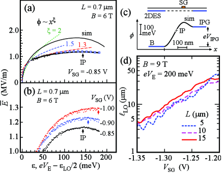
Figure 5: (a and b) Energy $\varepsilon$ dependence of $\bar{E}$. The data with open squares were obtained from the $B$-dependence, while other data with small dots were estimated from a single value of $\ell_{\mathrm{LO}}$. They were taken with a 0.7 $\mu$m device on wafer W2. The solid line in (a) is obtained from a self-consistent potential calculation shown in (c). The dashed lines represents the electric field for potential $\phi\propto x^{\xi}$ ($x>0$) with $\xi=$ 2, 1.5, and 1.3. The lower-energy data follows $\xi=$ 1.3. (c) Self-consistent potential profile $\phi$ for a realistic device geometry, shown in the upper inset, with $V_{\mathrm{SG}}=$ -0.85 V and $V_{\mathrm{IPG}}=$ -0.2 V. (d) $V_{\mathrm{SG}}$ dependence of $\ell_{\mathrm{LO}}$, taken with three devices ($L=$ 5, 10, and 15 $\mu$m) on wafer W1.

The energy ($eV_{\mathrm{E}}$) dependence of $\bar{E}$ is summarized in Figs. 5(a) and (b), where $\bar{E}$ is plotted as a function of the average energy $\bar{\varepsilon}=eV_{\mathrm{E}}-\varepsilon_{\mathrm{LO}}/2$ in the dLO transition. The data with open squares in (a) were obtained from the $B$-dependence, while other data with small dots in (a) and (b) were estimated from the measured $\ell_{\mathrm{LO}}$ and a fixed $\Gamma_{\mathrm{LO,0}}=$ 25 ps^-1. As clearly seen in the magnified plot of (b), $\bar{E}$ is maximized at $\bar{\varepsilon}\simeq$ 150 meV. This can be understood with a realistic potential profile between the base region and the IPG, as shown in Fig. 5(c). As the edge potential is defined by the surface gate (SG), there must be an inflection point (IP) with the maximum electric field. When $V_{\mathrm{SG}}$ is made less negative, electrostatics suggests that $\bar{E}$ at each $\varepsilon$ as well as the IP position in $\varepsilon$ decrease, which is consistent with the data in Fig. 5(b).

Our data is compared to the calculated electrostatic potential. Here, we have solved the Poisson equation with the boundary conditions around the 2DES and the gate. We used realistic device parameters; the 2DEG depth of 100 nm, the 2DEG thickness of 10 nm, the SG width of 80 nm, fixed surface charge and ionized donor concentrations that produce the surface potential and $n_{\mathrm{2DEG}}$, and applied voltages ($V_{\mathrm{SG}}$ = -0.85 V and $V_{\mathrm{IPG}}$ = 0.2 V). The obtained potential profile $\phi\left(x\right)$ is shown in Fig. 5(c), and its electric field is plotted with the solid line labeled ‘sim’ in Fig. 5(a). The simulation shows an IP at $\varepsilon\simeq$ 130 meV comparable to the measured one. The calculated electric field is somewhat greater than the experimental values, possibly due to imperfection of the model.

Figure 5(a) shows quite weak energy dependency of $\bar{E}$. Since $\bar{E}$ should be close to zero at zero energy (0.08 MV/m in Ref. McClurePRL2009 ), there must be a drastic change of $\bar{E}$ in the low-energy region ($<$ 20 meV). While the edge potential $\phi$ is often approximated by a quadratic form, this does not work well as shown by the dotted line (labelled $\xi=2$) for a quadratic potential with confinement energy of 5 meV. If we rely on a fully 2D model neglecting the thickness of the heterostructure, the edge potential has $\phi\propto x^{3/2}$ dependence in the lowest order near the edge channel, as suggested from Eq. (7) and (8) in Ref. Chklovskii . Our experimental data implies that the potential in the low energy range (20 $<$ $\varepsilon$ $<$ 60 meV) can be approximated with a power dependence $\phi\propto x^{\xi}$ for $x>0$, as shown by the dashed line with $\xi=1.3$. This energy dependency will be used in the analysis of electron-electron scattering.

For hot-electron applications, the LO phonon scattering can be suppressed by decreasing $\bar{E}$, which can be done with less negative $V_{\mathrm{SG}}$ as seen in Fig. 5(b). Actually, $\ell_{\mathrm{LO}}$ reaches about 30 $\mu$m at $B$ = 9 T by tuning $V_{\mathrm{SG}}$, as shown in Fig. 5(d) taken with several devices. Almost the same characteristics were reproduced with different $L$, which ensures the validity of our measurements.

V Electron-electron scattering

Next, we analyze the electron-electron interaction in the medium-energy region. This part of the data in Fig. 2 is replotted in Fig. 6(a), where the LO phonon scattering as well as the iLL process are not important. The hot-electron signal is clearly visible at $eV_{\mathrm{E}}>E_{\mathrm{th}}$ ($\simeq$ 25 meV), while the electron-hole excitation near $\varepsilon_{\det}=0$ is significant at $eV_{\mathrm{E}}<E_{\mathrm{th}}$. The latter is characterized by the excess current $\Delta I$ obtained at $\varepsilon_{\det}=0$ [see Fig. 2(a)]. Figure 6(b) shows the normalized excess current $\Delta I/I_{\mathrm{inj}}$ as a function of $V_{\mathrm{E}}$. It is maximized at $eV_{\mathrm{E}}\simeq$ 25 meV, which coincides with the vanishing point of the hot-electron signal. Therefore, we shall define $E_{\mathrm{th}}$ from the peak position in $\Delta I/I_{\mathrm{inj}}$. For $eV_{\mathrm{E}}<E_{\mathrm{th}}$, the hot electrons injected with energy $eV_{\mathrm{E}}$ are completely relaxed by exciting the Fermi sea, and the lost energy $\delta=eV_{\mathrm{E}}$ should contribute finite $\Delta I/I_{\mathrm{inj}}$. For $eV_{\mathrm{E}}>E_{\mathrm{th}}$, the hot electrons are partially relaxed by the energy loss $\delta$ ($<eV_{\mathrm{E}}$), which should contribute $\Delta I/I_{\mathrm{inj}}$. Even at higher energy $eV_{\mathrm{E}}>$ 60 meV, the hot electron peak in Fig. 6(a) is slightly deviated from the ballistic condition, and small but finite $\Delta I/I_{\mathrm{inj}}>0$ is seen in Fig. 6(b). They suggest the significance of electron-electron scattering even for nominally ballistic hot-electron transport.

For this problem, Lunde et al. have derived coupled Fokker-Plank equations for distribution functions in the two channels LundePRB2010-EE ; LundePRB-EE . For simplicity, we focus only on the average energy $\left\langle\varepsilon\right\rangle$ of hot electrons, provided that the hot electrons are energetically separated from the Fermi sea. Then, $\left\langle\varepsilon\right\rangle$ follows a simple differential equation

$$\frac{d}{dy}\left\langle\varepsilon\right\rangle=-\gamma\left(\left\langle\varepsilon\right\rangle\right),$$ (2)

if each collision provides infinitesimal energy exchange. Here, $\gamma\left(\varepsilon\right)$ is the energy relaxation rate per unit length along $y$ direction. If $\gamma$ were independent of $\varepsilon$ as assumed in Ref. LundePRB-EE , the energy loss $\delta=\gamma L$ for a fixed $L$ should have been independent of $\varepsilon$. Our result in Fig. 6(a) cannot be explained with a constant $\gamma$.

As we do not know the energy dependency of $\gamma\left(\varepsilon\right)$ at this stage, we assume that $\gamma$ can be written as $\gamma\left(\varepsilon\right)\simeq a\varepsilon^{-\lambda}$ with parameters $\lambda$ and $a$. This form is convenient as this provides an analytical solution of Eq. (2) and can be related to a physical model described later. With initial energy $\left\langle\varepsilon\right\rangle_{\mathrm{inj}}=eV_{\mathrm{E}}$, the final energy at $y=L$ follows

$$\left\langle\varepsilon\right\rangle_{L}=\left[\left(eV_{\mathrm{E}}\right)^{\lambda+1}-E_{\mathrm{th}}^{\lambda+1}\right]^{1/\left(\lambda+1\right)},$$ (3)

where

$$E_{\mathrm{th}}=\left[\left(\lambda+1\right)aL\right]^{1/\left(\lambda+1\right)}$$ (4)

is the threshold energy at which the hot electron just relaxes to the Fermi level. Figure 6(c) shows some calculated traces $\left\langle\varepsilon\right\rangle_{L}$ with $E_{\mathrm{th}}=$ 25 meV for several $\lambda=$ 0.5, 1, 2, and 4. We find $\lambda=$ 1 $\sim$ 1.5 reproduces the experimental data, as shown by the solid line with $\lambda=$ 1 overlaid in Fig. 6(a).

The electron-hole excitation can be analyzed with the excess current $\Delta I$ in Fig. 6(b). While the hot-electron spectroscopy works for energy greater than $w\simeq$ 5 meV, electron-hole plasma in the Fermi sea is distributed in a narrow energy range much smaller than $w$. Therefore, $\Delta I$ is based on thermoelectric current associated with the increased temperature. For simplicity, we assume that the electron-hole plasma is characterized by the Fermi distribution with an effective electron temperature $T_{\mathrm{eff}}$, which is greater than the base temperature $T_{\mathrm{base}}$ in the collector TwoStage-Itoh ; WashioPRB . If the lost energy $\delta$ is distributed to the two channels with a fraction $\beta$ for the spin-up channel ($\beta=\frac{1}{2}$ for equal energy distribution), the corresponding heat power $W=\beta\delta I_{\mathrm{inj}}/e$ determines the effective temperature as

$$T_{\mathrm{eff}}^{2}-T_{\mathrm{base}}^{2}=\frac{6h}{\pi^{2}k_{\mathrm{B}}^{2}}W$$ (5)

in the spin-up channel. As $k_{\mathrm{B}}T_{\mathrm{eff}}$ is always smaller than $w$ in our conditions, we can approximate that the tunneling probability of the detector, $T\left(\varepsilon\right)\simeq T_{0}+\frac{\varepsilon}{2w}$, changes from $T_{0}$ ($=\frac{1}{2}$ at $\varepsilon_{\mathrm{det}}=0$) linearly with small excess energy $\varepsilon$ ($\left|\varepsilon\right|\ll w$) with respect to the chemical potential $\mu_{\mathrm{B}}$. With this model the thermoelectric current through $\mathrm{P}_{\det}$ follows

$$I_{\mathrm{te}}\simeq\frac{\pi^{2}}{12w}\frac{e}{h}k_{\mathrm{B}}^{2}\left(T_{\mathrm{eff}}^{2}-T_{\mathrm{base}}^{2}\right),$$ (6)

for $k_{\mathrm{B}}T_{\mathrm{eff}}<w$. This yields the normalized thermal current $I_{\mathrm{te}}/I_{\mathrm{inj}}\simeq\frac{1}{2w}\beta\delta$.

However, $\Delta I$ in the measurement should be smaller than $I_{\mathrm{te}}$ in the presence of series resistance in our setup. As shown in the equivalent circuit between the base and the collector in the left inset to Fig. 7(b), finite current $\Delta I$ induces voltage drop in the contact resistance $R_{c}=\frac{h}{e^{2}}$ for the spin-up LLL and $Z_{\mathrm{m}}$ of the ammeters. A fraction of the thermoelectric current $I_{\mathrm{te}}$ flows back to the base through the tunneling resistance $R_{t}=\left(\frac{1}{T_{0}}-1\right)\frac{h}{e^{2}}$ of $\mathrm{P}_{\det}$ BookHeikkila . The other fraction

$$\eta=\frac{R_{t}}{R_{t}+R_{c}+2Z_{\mathrm{m}}}$$ (7)

of $I_{\mathrm{te}}$ is obtained in $\Delta I$ ($=\eta I_{\mathrm{te}}$) with our setup. Therefore, we find a simple relation

$$\Delta I/I_{\mathrm{inj}}=\frac{\eta\beta}{2w}\delta,$$ (8)

which relates $\Delta I/I_{\mathrm{inj}}$ in Fig. 6(b) and $\delta$ in Fig. 6(a). Note that this voltage drop is not important for hot electron spectroscopy with a higher barrier ($\eta=1$ with $T_{0}=0$ for Fermi sea) at $\varepsilon_{\mathrm{det}}\gg w$.

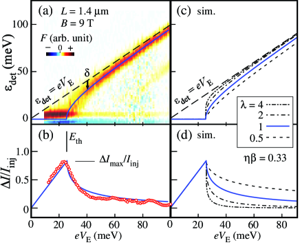
Figure 6: (a) The color-scale plot of $F\left(\varepsilon_{\det},V_{E}\right)$. The peak is deviated from the ballistic condition (the dashed line), and is explained well with the model calculation (the solid line at $\lambda=1$). (b) The obtained $\Delta I/I_{\mathrm{inj}}$ (solid circles) as a function of $eV_{E}$. The data is consistent with the model calculation (the solid line at $\lambda=1$) (c and d) The model calculation of hot-electron energy $\left\langle\varepsilon\right\rangle_{L}$ in (c) and $\Delta I/I_{\mathrm{inj}}$ in (d) for different $\lambda$.

If the average hot-electron energy follows Eq. (3) and the lines in Figs. 6(a) and 6(c), the corresponding $\Delta I/I_{\mathrm{inj}}$ should follow the lines in Figs. 6(b) and 6(d). Here, we chose $w=$ 5 meV and $\eta\beta=$ 0.33 to adjust the maximum $\Delta I/I_{\mathrm{inj}}$ to the experimental one. The parameter $\eta\beta$ [0.2 - 0.5 in Fig. 7(b)] is consistent with the equal heat distribution ($\beta=\frac{1}{2}$) and $\eta\simeq$ 0.4 for $T_{0}=$ 0.5 and $Z_{\mathrm{m}}=$ 10 k$\Omega$. The excellent agreement with the experimental data is found also in the high energy tail at $eV_{\mathrm{E}}>$ 40 meV. Namely, the both data sets in Figs. 6(a) and 6(b) are understood with the same energy loss $\delta$.

Figure 7 summarizes the $B$ dependence of $E_{\mathrm{th}}$ in (a) and the normalized peak value $\Delta I_{\mathrm{\max}}/I_{\mathrm{inj}}$ ($\Delta I/I_{\mathrm{inj}}$ at $\varepsilon=E_{\mathrm{th}}$) in (b) for several devices. The threshold energy $E_{\mathrm{th}}$ does not change with $B$ in Fig. 7(a). Weak $B$ dependence of $\Delta I_{\mathrm{\max}}/I_{\mathrm{inj}}$ is seen in Fig. 7(b). The $L$ dependence of $E_{\mathrm{th}}$ shown in the inset to Fig. 7(a) is consistent with Eq. (4); $E_{\mathrm{th}}\propto L^{0.4}$ $\sim$ $L^{0.5}$ (the dashed line) with $\lambda=1-1.5$.

In a standard electron-electron scattering model, a hot spin-up electron can relax by exchanging the energy with a cold spin-down electron or a cold spin-up electron, as depicted in Fig. 1(a). The latter process may be suppressed by the destructive interference with a similar process for exchanged final states LundePRB2010-EE , while such suppression should be incomplete in the presence of energy dependent relaxation rate $\gamma\left(\varepsilon\right)$. Nevertheless, spin-up and spin-down electrons in their Fermi seas are easily thermalized by the proximate interaction leSueurPRL2010 ; TwoStage-Itoh . This suggests equal heat distribution between the two channels ($\beta=\frac{1}{2}$) in agreement with the comparison in Fig. 6(b).

When the filling factor $\nu$ is increased above 2 ($B<$ 5.2 T), the heat can be distributed to electrons in the SLL. However, we did not see such characteristics in Figs. 7(a) and 7(b). If the hot electron scatters with electrons in the SLL [the dashed line in the right inset to Fig. 7(a)], the excess scattering should increase $E_{\mathrm{th}}$ at $\nu>2$. If the Fermi seas in the LLLs are interacting with electrons in the SLL [the dashed line in the right inset to Fig. 7(b)], the heat redistribution should decrease $\beta$ and thus $\Delta I_{\mathrm{\max}}/I_{\mathrm{inj}}$ at $\nu>2$. It seems both scattering processes with the SLL are negligible for the short length ($<$ 1.4 $\mu$m), possibly due to the large cyclotron energy that determines the channel distance between SLL and LLL as compared to the small Zeeman energy that determines the distance between spin-up and -down channels.

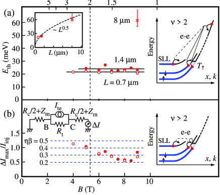
Figure 7: $B$ dependence of $E_{\mathrm{th}}$ in (a) and $\Delta I_{\mathrm{\max}}/I_{\mathrm{inj}}$ in (b) taken with several devices on wafer W2. The vertical dashed line shows the condition for $\nu$ = 2. The inset to (a) shows the interaction between a hot electron and electrons in the LLLs and the SLL at $\nu>$ 2. The right inset to (b) shows the interaction between the LLLs and the SLL. The left inset to (b) shows an equivalent circuit for relating $\Delta I$ with $I_{\mathrm{te}}$.

Now, we discuss the reason why the electron-electron scattering with $\gamma\left(\varepsilon\right)$ is suppressed with increasing energy. The electron-electron scattering should be sensitive to the potential profile $\phi\propto x^{\xi}$ ($\xi>0$) discussed with Fig. 5. A hot electron with higher energy $\varepsilon$ is more spatially separated from the Fermi sea (the distance $x\propto\varepsilon^{1/\xi}$). This appears in the Coulomb potential $U$ between the hot electron and an electron in the Fermi sea. If we ignore the screening effect from the gate metal, the bare Coulomb potential $U\propto x^{-1}\propto\varepsilon^{-1/\xi}$ decreases with increasing $\varepsilon$. Incidentally, the hot-electron velocity $v_{\mathrm{h}}$ is significantly greater than the Fermi velocity $v_{\mathrm{F}}$. With faster $v_{\mathrm{h}}$, the hot electron passes through the channel with less scattering in a shorter time. Moreover, electron-electron scattering should be suppressed with larger momentum mismatch proportional to $\left|v_{\mathrm{F}}^{-1}-v_{\mathrm{h}}^{-1}\right|$. All of these effects reduce the scattering of hot electrons with larger $\varepsilon$ and faster $v_{\mathrm{h}}$.

The scattering is allowed in the presence of random impurity potential, which fluctuates the Coulomb potential $U$ around the mean $U_{0}$ with the Fourier amplitude $A$ in the long-range limit over the correlation length $\ell_{p}$. In this case, $\gamma$ can be written as

$$\gamma=\frac{\hbar U_{0}^{2}Av_{\mathrm{F}}}{4\sqrt{2}\pi^{3/2}\ell_{p}^{3}v_{\mathrm{h}}^{2}}$$ (9)

in the limit of $v_{\mathrm{h}}\gg v_{\mathrm{F}}$, as derived in Eqs. (2) and (9) of Ref. LundePRB-EE . Since $A$, $\ell_{p}$, and $v_{\mathrm{F}}$ are irrelevant to the hot-electrons, $U_{0}$ ($\propto\varepsilon^{-1/\xi}$) and $v_{\mathrm{h}}$ ($=E/B\propto\varepsilon^{\left(\xi-1\right)/\xi}$) suggest the energy dependency of $\gamma\left(\varepsilon\right)\propto\varepsilon^{-2}$. This exponent is close to but somewhat larger than our experimental value of $\lambda=$ 1 $\sim$ 1.5 obtained for $\gamma\propto\varepsilon^{-\lambda}$ in Fig. 6.

It should be noted that Eq. (9) does not explain the absence of $B$ dependence of $E_{\mathrm{th}}$ in Fig. 7(a). If $v_{\mathrm{h}}$ and $v_{\mathrm{F}}$ have $1/B$ dependence, we expect a measurable $B$ dependence in $E_{\mathrm{th}}\propto\left(v_{\mathrm{F}}/v_{\mathrm{h}}^{2}\right)^{1/\left(\lambda+1\right)}$, which should exhibit $E_{\mathrm{th}}\propto B^{0.4}$ $\sim$ $B^{0.5}$ for $\lambda=$ 1 $\sim$ 1.5. The discrepancy might be related to the formation of many-body states in LLLs. At least, our previous work have shown that $v_{\mathrm{F}}$ is significantly enhanced by the Coulomb interaction with the Tomonaga-Luttinger model KumadaEMP ; KamataNatNano2014 . Such many-body states are not considered in the derivation of Eq. (9) LundePRB-EE . A single-particle hot electron scattering with many-body state may be worthy for studying non-linear hydrodynamic effect NonlinearTLL ; 1D2DTunSpectrum .

For hot-electron applications, the electron-electron scattering can be suppressed by decreasing $U_{0}$. This can be done with hotter electrons with longer distance from the Fermi sea or with screening effect by covering the surface with metal HotEDyQD-Kataoka .

VI Summary

In summary, we have investigated hot electron transport in the soft edge potential by means of hot electron spectroscopy. We find that the electron-electron interaction is suppressed for hotter electrons. The electron-phonon interaction is also suppressed by softening the edge potential. The observed ballistic hot-electron transport is attractive for utilizing hot electrons for studying electronic quantum optics.

- (1) B.K. Ridley, Quantum Processes in Semiconductors, Oxford Univ. Press, Oxford (1999).
- (2) G. F. Giuliani and J. J. Quinn, Phys. Rev. B 26, 4421-4428 (1982).
- (3) I. I. Kaya and K. Eberl, Phys. Rev. Lett. 98, 186801 (2007).
- (4) T. Karzig, L. I. Glazman and F. von Oppen, Phys Rev Lett 105, 226407 (2010).
- (5) U. Sivan, M. Heiblum, and C. P. Umbach, Phys. Rev. Lett. 63, 992 (1989).
- (6) U. Bockelmann and G. Bastard, Phys. Rev. B 42, 8947 (1990).
- (7) Yu. V. Nazarov and Y. M. Blanter, Quantum Transport - Introduction to Nanoscience, Cambridge Univ. Press, Cambridge (2009).
- (8) C. Rössler, S. Burkhard, T. Krähenmann, M. Röösli, P. Märki, J. Basset, T. Ihn, K. Ensslin, C. Reichl and W. Wegscheider, Phys Rev B 90, 081302 (2014).
- (9) Y. Ji, Y. C. Chung, D. Sprinzak, M. Heiblum, D. Mahalu and H. Shtrikman, Nature 422, 415 (2003).
- (10) V. Freulon, A. Marguerite, J. M. Berroir, B. Placais, A. Cavanna, Y. Jin and G. Feve, Nat Commun 6, 6854 (2015).
- (11) S. Tewari, P. Roulleau, C. Grenier, F. Portier, A. Cavanna, U. Gennser, D. Mailly and P. Roche, Phys. Rev. B 93, 035420 (2016).
- (12) H. le Sueur, C. Altimiras, U. Gennser, A. Cavanna, D. Mailly, and F. Pierre, Phys. Rev. Lett. 105, 056803 (2010).
- (13) M. Hashisaka, N. Hiyama, T. Akiho, K. Muraki and T. Fujisawa, Nature Physics 13, 559 (2017).
- (14) K. Itoh, R. Nakazawa, T. Ota, M. Hashisaka, K. Muraki, and T. Fujisawa, Phys. Rev. Lett. 120, 197701 (2018).
- (15) M. Kataoka, N. Johnson, C. Emary, P. See, J. P. Griffiths, G. A. C. Jones, I. Farrer, D. A. Ritchie, M. Pepper and T. J. B. M. Janssen, Phys Rev Lett 116, 126803 (2016).
- (16) J. D. Fletcher, P. See, H. Howe, M. Pepper, S. P. Giblin, J. P. Griffiths, G. A. C. Jones, I. Farrer, D. A. Ritchie, T. J. B. M. Janssen and M. Kataoka, Phys Rev Lett 111, 216807 (2013).
- (17) N. Ubbelohde, F. Hohls, V. Kashcheyevs, T. Wagner, L. Fricke, B. Kästner, K. Pierz, H. W. Schumacher and R. J. Haug, Nature Nanotech. 10, 46 (2015).
- (18) N. Johnson, C. Emary, S. Ryu, H.-S. Sim, P. See, J. D. Fletcher, J. P. Griffiths, G. A. C. Jones, I. Farrer, D. A. Ritchie, M. Pepper, T. J. B. M. Janssen, M. Kataoka, Phys. Rev. Lett. 121, 137703 (2018).
- (19) J. Reiner, A. K. Nayak, N. Avraham, A. Norris, B. Yan, I. C. Fulga, J.-H. Kang, T. Karzig, H. Shtrikman and H. Beidenkopf, Phys. Rev. X 7, 021016 (2017).
- (20) D. Taubert, G. J. Schinner, H. P. Tranitz, W. Wegscheider, C. Tomaras, S. Kehrein and S. Ludwig, Phys. Rev. B 82, 161416 (2010).
- (21) D. Taubert, G. J. Schinner, C. Tomaras, H. P. Tranitz, W. Wegscheider and S. Ludwig, J. Appl. Phys. 109, 102412 (2011).
- (22) D. Taubert, C. Tomaras, G. J. Schinner, H. P. Tranitz, W. Wegscheider, S. Kehrein and S. Ludwig, Phys Rev B 83, 235404 (2011).
- (23) Z. F. Ezawa, Quantum Hall Effects: Field Theorectical Approach and Related Topics (World Scientific Publishing, Singapore, 2008).
- (24) A. M. Lunde, S. E. Nigg and M. Büttiker, Phys Rev B 81, 041311 (2010).
- (25) A. M. Lunde and S. E. Nigg, Phys. Rev. B 94, 045409 (2016).
- (26) K. Washio, R. Nakazawa, M. Hashisaka, K. Muraki, Y. Tokura, and T. Fujisawa, Phys. Rev. B 93, 075304 (2016).
- (27) S. Komiyama, H. Hirai, M. Ohsawa, Y. Matsuda, S. Sasa and T. Fujii, Phys. Rev. B 45, 11085 (1992).
- (28) The probability of transport after emitting just phonons can also be used to estimate the relaxation length of partially relaxed hot electrons at . By solving the rate equations for the cascaded LO phonon emissions, can be estimated by using for . We find that does not contradict with obtained from , if they are compared for the same energy. However, the cascade analysis involves large uncertainty associated with the error accumulation.
- (29) N. Telang and S. Bandyopadhyay, Phys. Rev. B 48, 18002 (1993).
- (30) C. Emary, A. Dyson, S. Ryu, H. S. Sim and M. Kataoka, Phys. Rev. B 93, 035436 (2016).
- (31) The parameters are chosen to provide a comparable slope to the experimental data in the plot, while the significant bowing does not match the data.
- (32) D. T. McClure, Y. Zhang, B. Rosenow, E. M. Levenson-Falk, C. M. Marcus, L. N. Pfeiffer and K. W. West, Phys. Rev. Lett. 103, 206806 (2009).
- (33) D. B. Chklovskii, B. I. Shklovskii and L. I. Glazman, Phys Rev B 46 (7), 4026-4034 (1992).
- (34) T. T. Heikkilä, The Physics of Nanoelectronics (Oxford University Press, Oxford, England, 2013).
- (35) N. Kumada, H. Kamata, and T. Fujisawa, Phys. Rev. B 84, 045314 (2011).
- (36) H. Kamata, N. Kumada, M. Hashisaka, K. Muraki, and T. Fujisawa, Nature Nano. 9, 177 (2014).
- (37) A. Imambekov and L. I. Glazman, Science 323, 228 (2009).
- (38) O. Tsyplyatyev, A. J. Schofield, Y. Jin, M. Moreno, W. K. Tan, C. J. B. Ford, J. P. Griffiths, I. Farrer, G. A. C. Jones, and D. A. Ritchie, Phys. Rev. Lett. 114, 196401 (2015).