Streaming Low-Rank Matrix Approximation
with an Application to Scientific Simulation JAT was supported in part by ONR Awards N00014-11-1002, N00014-17-1-214, N00014-17-1-2146, and the Gordon & Betty Moore Foundation. MU was supported in part by DARPA Award FA8750-17-2-0101. VC has received funding from the European Research Council (ERC) under the European Union’s Horizon 2020 research and innovation programme under the grant agreement number 725594 (time-data) and the Swiss National Science Foundation (SNSF) under the grant number 200021_178865.

Abstract

This paper argues that randomized linear sketching is a natural tool for on-the-fly compression of data matrices that arise from large-scale scientific simulations and data collection. The technical contribution consists in a new algorithm for constructing an accurate low-rank approximation of a matrix from streaming data. This method is accompanied by an a priori analysis that allows the user to set algorithm parameters with confidence and an a posteriori error estimator that allows the user to validate the quality of the reconstructed matrix. In comparison to previous techniques, the new method achieves smaller relative approximation errors and is less sensitive to parameter choices. As concrete applications, the paper outlines how the algorithm can be used to compress a Navier–Stokes simulation and a sea surface temperature dataset.

Primary, 65F30; Secondary, 68W20.

1 Motivation

Computer simulations of scientific models often generate data matrices that are too large to store, process, or transmit in full. This challenge arises in a huge number of fields, including weather and climate forecasting [72, 25, 8], heat transfer and fluid flow [57, 10], computational fluid dynamics [9, 28], and aircraft design [51, 62]. Similar exigencies can arise with automated methods for acquiring large volumes of scientific data [19].

In these settings, the data matrix often has a decaying singular value spectrum, so it admits an accurate low-rank approximation. For some downstream applications, the approximation serves as well as—or even better than—the full matrix [64, 17]. Indeed, the approximation is easier to manipulate, and it can expose latent structure. This observation raises the question of how best to compute a low-rank approximation of a matrix of scientific data with limited storage, arithmetic, and communication.

The main purpose of this paper is to argue that sketching methods from the field of randomized linear algebra [74, 20, 35, 46, 73, 14, 29, 69, 68] have tremendous potential in this context. As we will explain, these algorithms can inexpensively maintain a summary, or sketch, of the data as it is being generated. After the data collection process terminates, we can extract a near-optimal low-rank approximation from the sketch. This approximation is accompanied by an a posteriori error estimate.

The second purpose of this paper is to design, analyze, and test a new sketching algorithm that is suitable for handling scientific data. We will build out the theoretical infrastructure needed for practitioners to deploy this algorithm with confidence. We will also demonstrate that the method is effective for some small- and medium-scale examples, including a computer simulation of the Navier–Stokes equations and a high-resolution sea surface temperature dataset [1].

1.1 Streaming, Sketching, and Matrix Approximation

Let us begin with a brief introduction to streaming data and sketching, as they apply to the problem of low-rank matrix approximation. This abstract presentation will solidify into a concrete algorithm in Sections 2 and 6. The explanation borrows heavily from our previous paper [69], which contains more details and context.

1.1.1 Streaming

We are interested in acquiring a compressed representation of an enormous matrix $\bm{A}\in\mathbb{F}^{m\times n}$ where $\mathbb{F}=\mathbb{R}$ or $\mathbb{F}=\mathbb{C}$. This work focuses on a setting where the matrix is presented as a long sequence of “simple” linear updates:

(1) $$\bm{A}=\bm{H}_{1}+\bm{H}_{2}+\bm{H}_{3}+\cdots.$$

In applications, each innovation $\bm{H}_{i}$ is sparse, low-rank, or enjoys another favorable structure. The challenge arises because we do not wish to store the full matrix $\bm{A}$, and we cannot revisit the innovation $\bm{H}_{i}$ after processing it. The formula Eq. 1 describes a particular type of streaming data model [53, 20, 73].

1.1.2 Sketching

To manage the data stream Eq. 1, we can use a randomized linear sketch [5, 4]. Before any data arrives, we draw and fix a random linear map $\mathscr{S}:\mathbb{F}^{m\times n}\to\mathbb{F}^{d}$, called a sketching operator. Instead of keeping $\bm{A}$ in working memory, we retain only the image $\mathscr{S}(\bm{A})$. This image is called a sketch of the matrix. The dimension $d$ of the sketch is much smaller than the dimension $mn$ of the matrix space, so the sketching operator compresses the data matrix. Nonetheless, because of the randomness, a well-designed sketching operator is likely to yield useful information about any matrix $\bm{A}$ that is statistically independent from $\mathscr{S}$.

Sketches and data streams enjoy a natural synergy. If the matrix $\bm{A}$ is presented via the data stream Eq. 1, the linearity of the sketching operator ensures that

$$\mathscr{S}(\bm{A})=\mathscr{S}(\bm{H}_{1})+\mathscr{S}(\bm{H}_{2})+\mathscr{S}(\bm{H}_{3})+\cdots.$$

In other words, we can process an innovation $\bm{H}_{i}$ by forming $\mathscr{S}(\bm{H}_{i})$ and adding it to the current value of the sketch. This update can be performed efficiently when $\bm{H}_{i}$ is structured. It is a striking fact [43] that randomized linear sketches are essentially the only mechanism for tracking a general data stream of the form (1).

1.1.3 Matrix Approximation

After the updating process terminates, we need to extract a low-rank approximation of the data matrix $\bm{A}$ from the sketch $\mathscr{S}(\bm{A})$. More precisely, we report a rank-$r$ matrix $\hat{\bm{A}}_{r}$, in factored form, that satisfies

(2) $$\|\bm{A}-\hat{\bm{A}}_{r}\|_{2}\approx\min_{\operatorname{rank}\bm{B}\leq r}\|\bm{A}-\bm{B}\|_{2},$$

where $\|\cdot\|_{2}$ is the Schatten 2-norm (also known as the Frobenius norm). We can also exploit the sketch to compute an a posteriori estimate of the error:

$$\mathrm{err}_{2}(\hat{\bm{A}}_{r})\approx\|\bm{A}-\hat{\bm{A}}_{r}\|_{2}.$$

This estimator helps us to select the precise rank $r$ of the approximation.

1.1.4 Goals

Our objective is to design a sketch rich enough to support these operations. Since a rank-$r$ matrix has about $2r(m+n)$ degrees of freedom, the sketch ideally should have size $d=\Theta(r(m+n))$. We want to compute the approximation using $\mathcal{O}(r^{2}(m+n))$ floating-point operations, the cost of orthogonalizing $r$ vectors.

Existing one-pass SVD algorithms (e.g., [74, 20, 35, 73, 15, 71, 69]) already meet these desiderata. Nevertheless, there remains room for improvement [69, Sec. 7.6].

1.1.5 Contributions

The main technical contribution of this paper is a new sketch-based algorithm for computing a low-rank approximation of a matrix from streaming data. The new algorithm is a hybrid of the methods from [71, Thm. 12] and [69, Alg. 7] that improves on the performance of its predecessors. Here are the key features of our work:

• The new method can achieve a near-optimal relative approximation Eq. 2 when the input matrix has a decaying singular value spectrum. In particular, our approach is more accurate than existing methods, especially when the storage budget is small. As a consequence, the new method delivers higher-quality estimates of leading singular vectors. (Section 7)

• The algorithm is accompanied by a priori error bounds that help us set the parameters of the sketch reliably. The new method is less sensitive to the choice of sketch parameters and to the truncation rank, as compared with existing methods. (Sections 5 and 7)

• Our toolkit includes an a posteriori error estimator for validating the quality of the approximation. This estimator also provides a principled mechanism for selecting the precise rank of the final approximation. (Section 6)

• The method treats the two matrix dimensions symmetrically. As a consequence, we can extend it to obtain an algorithm for low-rank Tucker approximation of a tensor from streaming data. See our follow-up paper [65].

For scientific simulation and data analysis, these advances are significant because they allow us to approximate the truncated singular value decomposition of a huge matrix accurately and with minimal resource usage.

1.2 Application to Scientific Simulation

As we have mentioned, it is often desirable to reduce scientific data before we submit it to further processing. This section outlines some of the techniques that are commonly used for this purpose, and it argues that randomized linear sketching may offer a better solution.

1.2.1 Dynamical Model for a Simulation

In many cases, we can model a simulation as a process that computes the state $\bm{a}_{t+1}\in\mathbb{F}^{m}$ of a system at time $t+1$ from the state $\bm{a}_{t}\in\mathbb{F}^{m}$ of the system at time $t$. We may collect the data generated by the simulation into a matrix $\bm{A}=[\bm{a}_{1},\dots,\bm{a}_{n}]\in\mathbb{F}^{m\times n}$. In scientific applications, it is common that this matrix has a decaying singular value spectrum.

The dimension $m$ of the state typically increases with the resolution of the simulation, and it can be very big. The time horizon $n$ can also be large, especially for problems involving multiple time scales and for “stiff” equations that have high sensitivity to numerical errors. In some settings, we may not even know the time horizon $n$ or the dimension $m$ of the state variable in advance.

1.2.2 On-the-Fly Compression via Sketching

Let us explain how sketching interacts with the dynamical model from Section 1.2.1 For simplicity, assume that the dimensions $m$ and $n$ of the data matrix $\bm{A}\in\mathbb{F}^{m\times n}$ are known. Draw and fix a randomized linear sketching operator $\mathscr{S}:\mathbb{F}^{m\times n}\to\mathbb{F}^{d}$.

We can view the dynamical model for the simulation as an instance of the data stream Eq. 1:

$$\bm{A}=\bm{a}_{1}\mathbf{e}_{1}^{*}+\bm{a}_{2}\mathbf{e}_{2}^{*}+\bm{a}_{3}\mathbf{e}_{3}^{*}+\cdots.$$

Here, $\mathbf{e}_{i}$ is the $i$th standard basis vector in $\mathbb{F}^{n}$. The sketch $\bm{x}=\mathscr{S}(\bm{A})\in\mathbb{F}^{d}$ evolves as

$$\bm{x}=\mathscr{S}(\bm{a}_{1}\mathbf{e}_{1}^{*})+\mathscr{S}(\bm{a}_{2}\mathbf{e}_{2}^{*})+\mathscr{S}(\bm{a}_{3}\mathbf{e}_{3}^{*})+\cdots.$$

Each time the simulation generates a new state $\bm{a}_{t}$, we update the sketch $\bm{x}$ to reflect the innovation $\bm{a}_{t}\mathbf{e}_{t}^{*}$ to the data matrix $\bm{A}$. We can exploit the fact that the innovation is a rank-one matrix to ensure that this computation has negligible incremental cost. After sketching the new state, we write it to external memory or simply discard it. Once the simulation is complete, we can extract a provably good low-rank approximation from the sketch, along with an error estimate.

1.2.3 Compression of Scientific Data: Current Art

At present, computational scientists rely on several other strategies for data reduction. One standard practice is to collect the full data matrix and then to compress it. Methods include direct computation of a low-rank matrix or tensor approximation [76, 6] or fitting a statistical model [18, 33, 47]. These approaches have high storage costs, and they entail communication of large volumes of data.

There are also some techniques for compressing simulation output as it is generated. One approach is to store only a subset of the columns of the data matrix (“snapshots” or “checkpointing”), instead of keeping the full trajectory [32, 37]. Another approach is to maintain a truncated singular value decomposition (SVD) using a rank-one updating method [16, 77]. Both techniques have the disadvantage that they do not preserve a complete, consistent view of the data matrix. The rank-one updating method also incurs a substantial computational cost at each step.

1.2.4 Contributions

We believe that randomized linear sketching resolves many of the shortcomings of earlier data reduction methods for scientific applications. We will show by example (Section 7) that our new sketching algorithm can be used to compress scientific data drawn from several applications:

• We apply the method to a 430 Megabyte (MB) data matrix from a direct numerical simulation, via the Navier–Stokes equations, of vortex shedding from a cylinder in a two-dimensional channel flow.

• The method is used to approximate a 1.1 Gigabyte (GB) temperature dataset collected at a network of weather stations in the northeastern United States.

• We can invoke the sketching algorithm as a module in an optimization algorithm for solving a large-scale phase retrieval problem that arises in microscopic imaging via Fourier ptychography. The full matrix would require over 5 GB of storage.

• As a larger-scale example, we show that our methodology allows us to compute an accurate truncated SVD of a sea surface temperature dataset, which requires over 75 GB in double precision. This experiment is performed without any adjustment of parameters or other retrospection.

These demonstrations support our assertion that sketching is a powerful tool for managing large-scale data from scientific simulations and measurement processes. We have written this paper to motivate computational scientists to consider sketching in their own applications.

1.3 Roadmap

In Section 2, we give a detailed presentation of the proposed method and its relationship to earlier work. We provide an informative mathematical analysis that explains the behavior of our algorithm (Section 5), and we describe how to construct a posteriori error estimates (Section 6). We also discuss implementation issues (Section 4), and we present extensive numerical experiments on real and simulated data (Section 7).

1.4 Notation

We use $\mathbb{F}$ for the scalar field, which is real $\mathbb{R}$ or complex $\mathbb{C}$. The symbol ^∗ refers to the (conjugate) transpose of a matrix or vector. The dagger ^† denotes the Moore–Penrose pseudoinverse. We write $\|\cdot\|_{p}$ for the Schatten $p$-norm for $p\in[1,\infty]$. The map $\llbracket{\cdot}\rrbracket_{r}$ returns any (simultaneous) best rank-$r$ approximation of its argument with respect to the Schatten $p$-norms [36, Sec. 6].

2 Sketching and Low-Rank Approximation of a Matrix

Let us describe the basic procedure for sketching a matrix and for computing a low-rank approximation from the sketch. We discuss prior work in Section 2.8. See Section 4 for implementation, Section 5 for parameter selection, and Section 6 for error estimation.

2.1 Dimension Reduction Maps

We will use dimension reduction to collect information about an input matrix. Assume that $d\leq N$. A randomized linear dimension reduction map is a random matrix $\bm{\Xi}\in\mathbb{F}^{d\times N}$ with the property that

(3) $$\operatorname{\mathbb{E}}\|\bm{\Xi}\bm{u}\|_{2}^{2}=\mathrm{const}\cdot\|\bm{u}\|_{2}^{2}\quad\text{for all $\bm{u}\in\mathbb{F}^{N}$.}$$

In other words, the map reduces a vector of dimension $N$ to dimension $d$, but it still preserves Euclidean distances on average. It is also desirable that we can store the map $\bm{\Xi}$ and apply it to vectors efficiently. See Section 3 for concrete examples.

2.2 The Input Matrix

Let $\bm{A}\in\mathbb{F}^{m\times n}$ be an arbitrary matrix that we wish to approximate. In many applications where sketching is appropriate, the matrix is presented implicitly as a sequence of linear updates; see Section 2.4.

To apply sketching methods for low-rank matrix approximation, the user needs to specify a target rank $r_{0}$. The target rank $r_{0}$ is a rough estimate for the final rank of the approximation, and it influences the choice of the sketch size. We can exploit a posteriori information to select the final rank; see Section 6.5.

Remark 2.1 (Unknown Dimensions).

For simplicity, we assume the matrix dimensions are known in advance. The framework can be modified to handle matrices with growing dimensions, such as a simulation with an unspecified time horizon.

2.3 The Sketch

Let us describe the sketching operators we use to acquire data about the input matrix. The sketching operators are parameterized by a “range” parameter $k$ and a “core” parameter $s$ that satisfy

$$r_{0}\leq k\leq s\leq\min\{m,n\},$$

where $r_{0}$ is the target rank. The parameter $k$ determines the maximum rank of an approximation. For now, be aware that the approximation scheme is more sensitive to the choice of $k$ than to the choice of $s$. In Section 5.4, we offer specific parameter recommendations that are supported by theoretical analysis. In Section 7.5, we demonstrate that these parameter choices are effective in practice.

Independently, draw and fix four randomized linear dimension reduction maps:

(4) $$\bm{\Upsilon} \in\mathbb{F}^{k\times m}\quad\text{and}\quad\bm{\Omega}\in\mathbb{F}^{k\times n};$$

$$\bm{\Phi} \in\mathbb{F}^{s\times m}\quad\text{and}\quad\bm{\Psi}\in\mathbb{F}^{s\times n}.$$

These dimension reduction maps are often called test matrices. The sketch itself consists of three matrices:

(5) $$\bm{X}:=\bm{\Upsilon}\bm{A}\in\mathbb{F}^{k\times n}\quad\text{and}\quad\bm{Y}:=\bm{A}\bm{\Omega}^{*}\in\mathbb{F}^{m\times k};$$

(6) $$\bm{Z}:=\bm{\Phi}\bm{A}\bm{\Psi}^{*}\in\mathbb{F}^{s\times s}.$$

The first two matrices $(\bm{X},\bm{Y})$ capture the co-range and the range of $\bm{A}$. The core sketch $(\bm{Z})$ contains fresh information that improves our estimates of the singular values and singular vectors of $\bm{A}$; it is responsible for the superior performance of the new method.

Remark 2.2 (Prior Work).

The paper [71, Sec. 3] contains the insight that a sketch of the form Eqs. 5 and 6 can support better low-rank matrix approximations, but it proposes a reconstruction algorithm that is less effective. Related (but distinct) sketches appear in the papers [74, 20, 35, 73, 23, 15, 70, 69].

2.4 Linear Updates

In streaming data applications, the input matrix $\bm{A}\in\mathbb{F}^{m\times n}$ is presented as a sequence of linear updates of the form

(7) $$\bm{A}\leftarrow\eta\bm{A}+\nu\bm{H}$$

where $\eta,\nu\in\mathbb{F}$ and the matrix $\bm{H}\in\mathbb{F}^{m\times n}$.

In view of the construction Eqs. 5 and 6, we can update the sketch $(\bm{X},\bm{Y},\bm{Z})$ of the matrix $\bm{A}$ to reflect the innovation Eq. 7 by means of the formulae

(8) $$\bm{X} \leftarrow\eta\bm{X}+\nu\bm{\Upsilon}\bm{H}$$

$$\bm{Y} \leftarrow\eta\bm{Y}+\nu\bm{H}\bm{\Omega}^{*}$$

$$\bm{Z} \leftarrow\eta\bm{Z}+\nu\bm{\Phi}\bm{H}\bm{\Psi}^{*}.$$

When implementing these updates, it is worthwhile to exploit favorable structure in the matrix $\bm{H}$, such as sparsity or low rank.

Remark 2.3 (Streaming Model).

For the linear update model Eq. 7, randomized linear sketches are more or less the only way to track the input matrix [43]. There are more restrictive streaming models (e.g., when the columns of the matrix are presented in sequence) where it is possible to design other types of algorithms [26, 29].

Remark 2.4 (Linearly Transformed Data).

We can use sketching to track any matrix that depends linearly on a data stream. Suppose that the input data $\bm{a}\in\mathbb{R}^{d}$, and we want to maintain the matrix $\mathscr{L}(\bm{a})$ induced by a fixed linear map $\mathscr{L}:\mathbb{F}^{d}\to\mathbb{F}^{m\times n}$. If we receive an update $\bm{a}\leftarrow\eta\bm{a}+\nu\bm{h}$, then the linear image evolves as $\mathscr{L}(\bm{a})\leftarrow\eta\mathscr{L}(\bm{a})+\nu\mathscr{L}(\bm{h})$. This update has the form (7), so we can apply the matrix sketch Eqs. 5 and 6 to track $\mathscr{L}(\bm{a})$ directly. This idea has applications to physical simulations where a known transform $\mathscr{L}$ exposes structure in the data [52].

2.5 Optional Step: Centering

Many applications require us to center the data matrix to remove a trend, such as the temporal average. Principal component analysis (PCA) also involves a centering step [42]. For superior accuracy, it is wise to perform this operation before sketching the matrix.

As an example, let us explain how to compute and remove the mean value of each row of the data matrix in the streaming setting. We can maintain an extra vector $\bm{\mu}\in\mathbb{F}^{m}$ that tracks the mean value of each row. To process an update of the form Eq. 7, we first apply the steps

$$\bm{h}\leftarrow n^{-1}\bm{H}\mathbf{e}\quad\text{and}\quad\bm{H}\leftarrow\bm{H}-\bm{h}\mathbf{e}^{*}\quad\text{and}\quad\bm{\mu}\leftarrow\eta\bm{\mu}+\nu\bm{h}.$$

Here, $\mathbf{e}\in\mathbb{F}^{n}$ is the vector of ones. Afterward, we update the sketches using Eq. 8. The sketch now contains the centered data matrix, where each row has zero mean.

2.6 Computing Truncated Low-Rank Approximations

Once we have acquired a sketch $(\bm{X},\bm{Y},\bm{Z})$ of the input matrix $\bm{A}$, we must produce a good low-rank approximation. Let us outline the computations we propose. The intuition appears below in Section 2.7, and Section 5 presents a theoretical analysis.

The first two components $(\bm{X},\bm{Y})$ of the sketch are used to estimate the co-range and the range of the matrix $\bm{A}$. Compute thin QR factorizations:

(9) $$\bm{X}^{*}=:\bm{P}\bm{R}_{1}\quad\text{where}\quad\bm{P}\in\mathbb{F}^{n\times k};$$

$$\bm{Y}=:\bm{Q}\bm{R}_{2}\quad\text{where}\quad\bm{Q}\in\mathbb{F}^{m\times k}.$$

Both $\bm{P}$ and $\bm{Q}$ have orthonormal columns; discard the triangular parts $\bm{R}_{1}$ and $\bm{R}_{2}$.

The third sketch $\bm{Z}$ is used to compute the core approximation $\bm{C}$, which describes how $\bm{A}$ acts between $\operatorname{range}(\bm{P})$ and $\operatorname{range}(\bm{Q})$:

(10) $$\bm{C}:=(\bm{\Phi Q})^{\dagger}\bm{Z}((\bm{\Psi}\bm{P})^{\dagger})^{*}\in\mathbb{F}^{k\times k}.$$

This step is implemented by solving a family of least-squares problems.

Next, form a rank-$k$ approximation $\hat{\bm{A}}$ of the input matrix $\bm{A}$ via

(11) $$\hat{\bm{A}}:=\bm{Q}\bm{C}\bm{P}^{*}$$

We refer to $\hat{\bm{A}}$ as the “initial” approximation. It is important to be aware that the initial approximation can contain spurious information (in its smaller singular values and the associated singular vectors).

To produce an approximation that is fully reliable, we must truncate the rank of the initial approximation Eq. 11. For a truncation parameter $r$, we construct a rank-$r$ approximation by replacing $\hat{\bm{A}}$ with its best rank-$r$ approximation in Frobenius norm:

(12) $$\llbracket{\hat{\bm{A}}}\rrbracket_{r}=\bm{Q}\llbracket{\bm{C}}\rrbracket_{r}\bm{P}^{*}.$$

We refer to $\llbracket{\hat{\bm{A}}}\rrbracket_{r}$ as a “truncated” approximation. Section 6.5 outlines some ways to use a posteriori information to select the truncation rank $r$.

The truncation Eq. 12 has an appealing permanence property: $\llbracket{\llbracket{\hat{\bm{A}}}\rrbracket_{\varrho}}\rrbracket_{r}=\llbracket{\hat{\bm{A}}}\rrbracket_{r}$ for all $\varrho\geq r$. In other words, the rank-$r$ approximation persists as part of all higher-rank approximations. In contrast, some earlier reconstruction methods are unstable in the sense that the rank-$r$ approximation varies wildly with $r$; see Section D.7.

Remark 2.5 (Extensions).

We can form other structured approximations of $\bm{A}$ by projecting $\hat{\bm{A}}$ onto a set of structured matrices. See [69, Secs. 5–6] for a discussion of this idea in the context of another sketching technique. For brevity, we do not develop this point further. See our paper [68] for a sketching and reconstruction method designed specifically for positive-semidefinite matrices.

Remark 2.6 (Prior Work).

The truncated approximation Eq. 12 is new, but it depends on insights from our previous work [70, 69]. Upadhyay [71, Thm. 12] proposes a different reconstruction formula for the same kind of sketch. The papers [74, 20, 35, 73, 23, 15, 71] describe other methods for low-rank matrix approximation from a randomized linear sketch. The numerical work in Section 7 demonstrates that Eq. 12 matches or improves on earlier techniques.

2.7 Intuition

The approximations Eqs. 11 and 12 are based on some well-known insights from randomized linear algebra [35, Sec. 1]. Since $\bm{P}$ and $\bm{Q}$ capture the co-range and range of the input matrix, we expect that

(13) $$\bm{A}\approx\bm{Q}(\bm{Q}^{*}\bm{A}\bm{P})\bm{P}^{*}$$

(See Lemma A.5 for justification.) We cannot compute the core matrix $\bm{Q}^{*}\bm{A}\bm{P}$ directly from a linear sketch because $\bm{P}$ and $\bm{Q}$ are functions of $\bm{A}$. Instead, we estimate the core matrix using the core sketch $\bm{Z}$. Owing to the approximation Eq. 13,

$$\bm{Z}=\bm{\Phi}\bm{A}\bm{\Psi}^{*}\approx(\bm{\Phi Q})(\bm{Q}^{*}\bm{A}\bm{P})(\bm{P}^{*}\bm{\Psi}^{*}).$$

Transfer the outer matrices to the left-hand side to discover that the core approximation $\bm{C}$, defined in (10), satisfies

(14) $$\bm{C}=(\bm{\Phi Q})^{\dagger}\bm{Z}((\bm{\Psi}\bm{P})^{\dagger})^{*}\approx\bm{Q}^{*}\bm{A}\bm{P}.$$

In view of Eqs. 13 and 14, we arrive at the relations

$$\bm{A}\approx\bm{Q}(\bm{Q}^{*}\bm{A}\bm{P})\bm{P}^{*}\approx\bm{Q}\bm{C}\bm{P}^{*}=\hat{\bm{A}}.$$

The error in the last relation depends on the error in the best rank-$k$ approximation of $\bm{A}$. When $\bm{A}$ has a decaying spectrum, the rank-$r$ truncation of $\bm{A}$ for $r\ll k$ agrees closely with the rank-$r$ truncation of the initial approximation $\hat{\bm{A}}$. That is,

$$\llbracket{\bm{A}}\rrbracket_{r}\approx\llbracket{\hat{\bm{A}}}\rrbracket_{r}=\bm{Q}\llbracket{\bm{C}}\rrbracket_{r}\bm{P}^{*}.$$

Theorems 5.1 and 5.5 justify these heuristics completely for Gaussian dimension reduction maps. Section 6.5 discusses a posteriori selection of $r$.

2.8 Discussion of Related Work

Sketching algorithms are specifically designed for the streaming model; that is, for data that is presented as a sequence of updates. The sketching paradigm is attributed to [5, 4]; see the survey [53] for an introduction and overview of early work.

Randomized algorithms for low-rank matrix approximation were proposed in the theoretical computer science (TCS) literature in the late 1990s [56, 27]. Soon after, numerical analysts developed practical versions of these algorithms [49, 74, 60, 35, 34]. For more background on the history of randomized linear algebra, see [35, 46, 73].

The paper [74] contains the first one-pass algorithm for low-rank matrix approximation; it was designed to control communication and arithmetic costs, rather than to handle streaming data. The first general treatment of numerical linear algebra in the streaming model appears in [20]. Recent papers on low-rank matrix approximation in the streaming model include [15, 71, 26, 29, 69, 68].

2.8.1 Approaches from NLA

The NLA literature contains a number of papers [74, 35, 69] on low-rank approximation from a randomized linear sketch. These methods all compute the range matrix $\bm{Q}$ and the co-range matrix $\bm{P}$ using the randomized range finder [35, Alg. 4.1], encapsulated in Eqs. 5 and 9.

The methods differ in how they construct a core matrix $\tilde{\bm{C}}$ so that $\bm{A}\approx\bm{Q}\tilde{\bm{C}}\bm{P}$. Earlier papers reuse the range and co-range sketches ($\bm{X}$, $\bm{Y}$) and the associated test matrices ($\bm{\Upsilon}$, $\bm{\Omega}$) to form $\tilde{\bm{C}}$. Our new algorithm is based on an insight from [15, 71] that the estimate $\bm{C}$ from Eq. 10 is more reliable because it uses a random sketch $\bm{Z}$ that is statistically independent from ($\bm{X}$, $\bm{Y}$). The storage cost of the additional sketch is negligible when $s^{2}\ll k(m+n)$.

The methods also truncate the rank of the approximation at different steps. The older papers [74, 35] perform the truncation before estimating the core matrix (cf. Section D.1.1). One insight from [69] is that it is beneficial to perform the truncation after estimating the core matrix. Furthermore, an effective truncation mechanism is to report a best rank-$r$ approximation of the initial estimate. We have adopted the latter approach.

2.8.2 Approaches from TCS

Most of the algorithms in the TCS literature [20, 73, 23, 15, 71] are based on a framework called “sketch-and-solve” that is attributed to Sarlós [63]. The basic idea is that the solution to a constrained least-squares problem (e.g., low-rank matrix approximation in Frobenius norm) is roughly preserved when we solve the problem after randomized linear dimension reduction.

The sketch-and-solve framework sometimes leads to the same algorithms as the NLA point of view; other times, it leads to different approaches. It would take us too far afield to detail these derivations, but we give a summary of one such method [71, Thm. 12] in Section D.1.3. Unfortunately, sketch-and-solve algorithms are often unsuitable for high-accuracy computations; see Section 7 and [69, Sec. 7] for evidence.

A more salient criticism is that the TCS literature does not attend to the issues that arise if we want to use sketching algorithms in practice. We have expended a large amount of effort to address these challenges, which range from parameter selection to numerically sound implementation. See [69, Sec. 1.7.4] for more discussion.

3 Randomized Linear Dimension Reduction Maps

In this section, we describe several randomized linear dimension reduction maps that are suitable for implementing sketching algorithms for low-rank matrix approximation. See [44, 35, 73, 69, 66] for additional discussion and examples. The class template for a dimension reduction map appears as Algorithm 1; the algorithms for specific dimension reduction techniques are postponed to the supplement.

Algorithm 1 Dimension Reduction Map Class.

1class DimRedux ($\mathbb{F}$) $\triangleright$ Dimension reduction map over field $\mathbb{F}$

2     function DimRedux($d,N$) $\triangleright$ Construct map $\bm{\Xi}:\mathbb{F}^{N}\to\mathbb{F}^{d}$      

3     function DimRedux.mtimes(DRmap, $\bm{M}$) $\triangleright$ Left action of map      

4     function DimRedux.mtimes($\bm{M},\texttt{DRmap}^{*}$) $\triangleright$ Right action of adjoint

5         return $(\textsc{DimRedux.mtimes}(\texttt{DRmap},\bm{M}^{*}))^{*}$ $\triangleright$ Default behavior      

3.1 Gaussian Maps

The most basic dimension reduction map is simply a Gaussian matrix. That is, $\bm{\Xi}\in\mathbb{F}^{d\times N}$ is a $d\times N$ matrix with independent standard normal entries.

Algorithm 7 describes an implementation of Gaussian dimension reduction. The map $\bm{\Xi}$ requires storage of $dN$ floating-point numbers in the field $\mathbb{F}$. The cost of applying the map to a vector is $\mathcal{O}(dN)$ arithmetic operations.

Gaussian dimension reduction maps are simple, and they are effective in randomized algorithms for low-rank matrix approximation [35]. We can also analyze their behavior in full detail; see Sections 5 and 6. On the other hand, it is expensive to draw a large number of Gaussian random variables, and the cost of storage and arithmetic renders these maps less appealing when the output dimension $d$ is large.

Remark 3.1 (Unknown Dimension).

Since the columns of a Gaussian map $\bm{\Xi}$ are statistically independent, we can instantiate more columns if we need to apply $\bm{\Xi}$ to a longer vector. Sparse maps (Section 3.3) share this feature. This observation is valuable in the streaming setting, where a linear update might involve coordinates heretofore unseen, forcing us to enlarge the domain of the dimension reduction map.

Remark 3.2 (History).

Gaussian dimension reduction has been used as an algorithmic tool since the paper [40] of Indyk & Motwani. In spirit, this approach is quite similar to the earlier theoretical work of Johnson & Lindenstrauss [41], which performs dimension reduction by projection onto a random subspace.

3.2 Scrambled SRFT Maps

Next, we describe a structured dimension reduction map, called a scrambled subsampled randomized Fourier transform (SSRFT). We recommend this approach for practical implementations.

An SSRFT map takes the form

$$\bm{\Xi}=\bm{RF\Pi F\Pi}^{\prime}\in\mathbb{F}^{d\times N}.$$

The matrices $\bm{\Pi},\bm{\Pi}^{\prime}\in\mathbb{F}^{N\times N}$ are signed permutations, drawn independently and uniformly at random. The matrix $\bm{F}\in\mathbb{F}^{N\times N}$ denotes a discrete cosine transform $(\mathbb{F}=\mathbb{R})$ or a discrete Fourier transform $(\mathbb{F}=\mathbb{C})$. The matrix $\bm{R}\in\mathbb{F}^{d\times N}$ is a restriction to $d$ coordinates, chosen uniformly at random.

Algorithm 8 presents an implementation of an SSRFT. The cost of storing $\bm{\Xi}$ is just $\mathcal{O}(N)$ numbers. The cost of applying $\bm{\Xi}$ to a vector is $\mathcal{O}(N\log N)$ arithmetic operations, using the Fast Fourier Transform (FFT) or the Fast Cosine Transform (FCT). According to [74], this cost can be reduced to $\mathcal{O}(N\log d)$, but the improvement is rarely worth the implementation effort.

In practice, SSRFTs behave slightly better than Gaussian matrices, even though their storage cost does not scale with the output dimension $d$. On the other hand, the analysis [3, 67, 13] is less complete than in the Gaussian case [35]. A proper implementation requires fast trigonometric transforms. Last, the random permutations and FFTs require data movement, which could be a challenge in the distributed setting.

Remark 3.3 (History).

SSRFTs are inspired by the work of Ailon & Chazelle [3] on fast Johnson–Lindstrauss transforms. For applications in randomized linear algebra, see the papers [74, 44, 35, 67, 13].

3.3 Sparse Sign Matrices

Last, we describe another type of randomized dimension reduction map, called a sparse sign matrix. We recommend these maps for practical implementations where data movement is a concern.

To construct a sparse sign matrix $\bm{\Xi}\in\mathbb{F}^{d\times N}$, we fix a sparsity parameter $\zeta$ in the range $2\leq\zeta\leq d$. The columns of the matrix are drawn independently at random. To construct each column, we take $\zeta$ iid draws from the $\textsc{uniform}\{z\in\mathbb{F}:|z|=1\}$ distribution, and we place these random variables in $p$ coordinates, chosen uniformly at random. Empirically, we have found that $\zeta=\min\{d,8\}$ is a very reliable parameter selection in the context of low-rank matrix approximation.

Algorithm 9 describes an implementation of sparse dimension reduction. Since the matrix $\bm{\Xi}\in\mathbb{F}^{d\times N}$ has $\zeta$ nonzeros per column, we can store the matrix with $\mathcal{O}(\zeta N\log(1+d/\zeta))$ numbers via run-length coding. The cost of applying the map to a vector is $\mathcal{O}(\zeta N)$ arithmetic operations.

Sparse sign matrices can reduce data movement because the columns are generated independently and the matrices can be applied using (blocked) matrix multiplication. They can also adapt to input vectors whose maximum dimension $N$ may be unknown, as discussed in Remark 3.1. One weakness is that we must use sparse data structures and arithmetic to enjoy the benefit of these maps.

Remark 3.4 (History).

Sparse dimension reduction maps are inspired by the work of Achlioptas [2] on database-friendly random projections. For applications in randomized linear algebra, see [21, 50, 54, 55, 12]. See [22] for a theoretical analysis in the context of matrix approximation.

4 Implementation and Costs

This section contains further details about the implementation of the sketching and reconstruction methods from Section 2, including an account of storage and arithmetic costs. We combine the mathematical notation from the text with Matlab R2018b commands (typewriter font). The electronic materials include a Matlab implementation of these methods.

4.1 Sketching and Updates

Algorithms 2 and 3 contain the pseudocode for initializing the sketch and for performing the linear update Eq. 7. It also includes optional code for maintaining an error sketch (Section 6).

The sketch requires storage of four dimension reduction maps with size $k\times m$, $k\times n$, $s\times m$, $s\times n$. We recommend using SSRFTs or sparse sign matrices to minimize the storage costs associated with the dimension reduction maps.

The sketch itself consists of three matrices with dimensions $k\times n$, $m\times k$, and $s\times s$. In general, the sketch matrices are dense, so they require $k(m+n)+s^{2}$ floating-point numbers in the field $\mathbb{F}$.

The arithmetic cost of the linear update $\bm{A}\leftarrow\eta\bm{A}+\tau\bm{H}$ is dominated by the cost of computing $\bm{\Phi H}$ and $\bm{H\Psi}$. In practice, the innovation $\bm{H}$ is low-rank, sparse, or structured. The precise cost of the update depends on how we exploit the structure of $\bm{H}$ and the dimension reduction map.

Algorithm 2 Sketch Constructor. Implements Eqs. 4, 5, 6, and 23

1Field $\mathbb{F}$; input matrix dimensions $m\times n$; approximation sketch size parameters $k\leq s\leq\min\{m,n\}$; error sketch size parameter $q$

2Draw test matrices for the approximation Eq. 4 and the error estimate Eq. 22; form the sketch Eqs. 5, 6, and 23 of the zero matrix $\bm{A}=\bm{0}$

3class Sketch

4     local variables $\bm{\Upsilon},\bm{\Omega},\bm{\Phi},\bm{\Psi}$ (DimRedux)

5     local variables $\bm{X},\bm{Y},\bm{Z}$ (matrices)

6     local variables $\bm{\Theta}$ (GaussDR), $\bm{W}$ (matrix) $\triangleright$ [opt] For error estimation

7     function Sketch($m,n,k,s,q$; DR) $\triangleright$ Constructor; DR is a DimRedux

8         $\bm{\Upsilon}\leftarrow\textsc{DR}(k,m)$ $\triangleright$ Construct test matrix for range

9         $\bm{\Omega}\leftarrow\textsc{DR}(k,n)$ $\triangleright$ Test matrix for co-range

10         $\bm{\Phi}\leftarrow\textsc{DR}(s,m)$ $\triangleright$ Test matrices for core

11         $\bm{\Psi}\leftarrow\textsc{DR}(s,n)$

12         $\bm{\Theta}\leftarrow\textsc{GaussDR}(q,m)$ $\triangleright$ [opt] Gaussian test matrix for error

13         $\bm{X}\leftarrow\texttt{zeros}(k,n)$ $\triangleright$ Approximation sketch of zero matrix

14         $\bm{Y}\leftarrow\texttt{zeros}(m,k)$

15         $\bm{Z}\leftarrow\texttt{zeros}(s,s)$

16         $\bm{W}\leftarrow\texttt{zeros}(q,n)$ $\triangleright$ [opt] Error sketch of zero matrix      

Algorithm 3 Linear Update to Sketch. Implements Eqs. 7 and 24.

1Innovation $\bm{H}\in\mathbb{F}^{m\times n}$; scalars $\eta,\nu\in\mathbb{F}$

2Modifies sketch to reflect linear update $\bm{A}\leftarrow\eta\bm{A}+\nu\bm{H}$

3function Sketch.LinearUpdate($\bm{H};\eta,\nu$)

4     $\bm{X}\leftarrow\eta\bm{X}+\nu\bm{\Upsilon H}$ $\triangleright$ Update range sketch

5     $\bm{Y}\leftarrow\eta\bm{Y}+\nu\bm{H\Omega}^{*}$ $\triangleright$ Update co-range sketch

6     $\bm{Z}\leftarrow\eta\bm{Z}+\nu(\bm{\Phi H})\bm{\Psi}^{*}$ $\triangleright$ Update core sketch

7     $\bm{W}\leftarrow\eta\bm{W}+\nu\bm{\Theta H}$ $\triangleright$ [opt] Update error sketch

4.2 The Initial Approximation

Algorithm 4 lists the pseudocode for computing a rank-$k$ approximation $\hat{\bm{A}}$ of the matrix $\bm{A}$ contained in the sketch; see Eq. 11.

The method requires additional storage of $k(m+n)$ numbers for the orthonormal matrices $\bm{P}$ and $\bm{Q}$, as well as $\mathcal{O}(sk)$ numbers to form the core matrix $\bm{C}$. The arithmetic cost is usually dominated by the computation of the QR factorizations of $\bm{X}^{*}$ and $\bm{Y}$, which require $\mathcal{O}(k^{2}(m+n))$ operations. When the parameters satisfy $s\gg k$, it is possible that the cost $\mathcal{O}(ks^{2})$ of forming the core matrix $\bm{C}$ will dominate; bear this in mind when setting the parameter $s$.

4.3 The Truncated Approximation

Algorithm 5 presents the pseudocode for computing a rank-$r$ approximation $\llbracket{\hat{\bm{A}}}\rrbracket_{r}$ of the matrix $\bm{A}$ contained in the sketch; see Eq. 12. The parameter $r$ is an input; the output is presented as a truncated SVD.

The working storage cost $\mathcal{O}(k(m+n))$ is dominated by the call to Algorithm 4. Typically, the arithmetic cost is also dominated by the $\mathcal{O}(k^{2}(m+n))$ cost of the call to Algorithm 4. When $s\gg k$, we need to invoke a randomized SVD algorithm [35] to achieve this arithmetic cost, but an ordinary dense SVD sometimes serves.

Algorithm 4 Initial Approximation. Implements Eq. 11.

1Rank-$k$ approximation of sketched matrix in the form $\hat{\bm{A}}=\bm{QCP}^{*}$ with orthonormal $\bm{Q}\in\mathbb{F}^{m\times k}$ and $\bm{P}\in\mathbb{F}^{n\times k}$ and $\bm{C}\in\mathbb{F}^{k\times k}$

2function Sketch.InitialApprox( )

3     $(\bm{Q},\sim)\leftarrow\texttt{qr}(\bm{Y},\texttt{0})$ $\triangleright$ Compute orthogonal part of thin QR

4     $(\bm{P},\sim)\leftarrow\texttt{qr}(\bm{X}^{*},\texttt{0})$

5     $\bm{C}\leftarrow((\bm{\Phi Q})\backslash\bm{Z})/((\bm{\Psi P})^{*})$ $\triangleright$ Solve two least-squares problems

6     return $(\bm{Q},\bm{C},\bm{P})$

Algorithm 5 Truncated Approximation. Implements Eq. 12.

1Final rank $r$ of the approximation

2Rank-$r$ approximation of sketched matrix in the form $\hat{\bm{A}}_{r}=\bm{U\Sigma V}^{*}$ with orthonormal $\bm{U}\in\mathbb{F}^{m\times r}$ and $\bm{V}\in\mathbb{F}^{n\times r}$ and nonnegative diagonal $\bm{\Sigma}\in\mathbb{R}^{r\times r}$

3function Sketch.TruncateApprox($r$)

4     $(\bm{Q},\bm{C},\bm{P})\leftarrow\textsc{Sketch.InitialApprox}(\,)$

5     $(\bm{U},\bm{\Sigma},\bm{V})\leftarrow\texttt{svd}(\bm{C})$ $\triangleright$ Dense or randomized SVD

6     $\bm{\Sigma}\leftarrow\bm{\Sigma}(\texttt{1:r},\texttt{1:r})$ $\triangleright$ Truncate SVD to rank $r$

7     $\bm{U}\leftarrow\bm{U}(\texttt{:},\texttt{1:r})$

8     $\bm{V}\leftarrow\bm{V}(\texttt{:},\texttt{1:r})$

9     $\bm{U}\leftarrow\bm{Q}\bm{U}$ $\triangleright$ Consolidate unitary factors

10     $\bm{V}\leftarrow\bm{P}\bm{V}$

11     return $(\bm{U},\bm{\Sigma},\bm{V})$

5 A Priori Error Bounds

It is always important to characterize the behavior of numerical algorithms, but the challenge is more acute for sketching methods. Indeed, we cannot store the stream of updates, so we cannot repeat the computation with new parameters if it is unsuccessful. As a consequence, we must perform a priori theoretical analysis to be able to implement sketching algorithms with confidence.

In this section, we analyze the low-rank reconstruction algorithms in the ideal case where all of the dimension reduction maps are standard normal. These results allow us to make concrete recommendations for the sketch size parameters. Empirically, other types of dimension reduction exhibit almost identical performance (Section 7.4), so our analysis also supports more practical implementations based on SSRFTs or sparse sign matrices. The numerical work in Section 7 confirms the value of this analysis.

5.1 Notation

For each integer $r\geq 0$, the tail energy of the input matrix is

$$\tau_{r+1}^{2}(\bm{A}):=\min_{\operatorname{rank}(\bm{B})\leq r}\|\bm{A}-\bm{B}\|_{2}^{2}=\|\bm{A}-\llbracket{\bm{A}}\rrbracket_{r}\|_{2}^{2}=\sum\nolimits_{j>r}\sigma_{j}^{2}(\bm{A}),$$

where $\sigma_{j}$ returns the $j$th largest singular value of a matrix. The second identity follows from the Eckart–Young Theorem [36, Sec. 6].

We also introduce parameters that reflect the field over which we are working:

(15) $$\alpha:=\alpha(\mathbb{F}):=\begin{cases}1,&\mathbb{F}=\mathbb{R}\\ 0,&\mathbb{F}=\mathbb{C}\end{cases}\quad\text{and}\quad\beta:=\beta(\mathbb{F}):=\begin{cases}1,&\mathbb{F}=\mathbb{R}\\ 2,&\mathbb{F}=\mathbb{C}.\end{cases}$$

These quantities let us present real and complex results in a single formula.

5.2 Analysis of Initial Approximation

The first result gives a bound for the expected error in the initial rank-$k$ approximation $\hat{\bm{A}}$ of the input matrix $\bm{A}$.

Theorem 5.1 (Initial Approximation: Error Bound).

Let $\bm{A}\in\mathbb{F}^{m\times n}$ be an arbitrary input matrix. Assume the sketch size parameters satisfy $s\geq 2k+\alpha$. Draw independent Gaussian dimension reduction maps $(\bm{\Upsilon},\bm{\Omega},\bm{\Phi},\bm{\Psi})$, as in Eq. 4. Extract a sketch Eqs. 5 and 6 of the input matrix. Then the rank-$k$ approximation $\hat{\bm{A}}$, constructed in Eq. 11, satisfies the error bound

(16) $$\operatorname{\mathbb{E}}\|\bm{A}-\hat{\bm{A}}\|_{2}^{2}\leq\frac{s-\alpha}{s-k-\alpha}\cdot\min_{\varrho<k-\alpha}\frac{k+\varrho-\alpha}{k-\varrho-\alpha}\cdot\tau_{\varrho+1}^{2}(\bm{A}).$$

We postpone the proof to Appendix A. The analysis is similar in spirit to the proof of [69, Thm. 4.3], but it is somewhat more challenging.

Theorem 5.1 contains explicit and reasonable constants, so we can use it to design algorithms that achieve a specific error tolerance. For example, suppose that $r_{0}$ is the target rank of the approximation. Then the choice

(17) $$k=4r_{0}+\alpha\quad\text{and}\quad s=2k+\alpha$$

ensures that the expected error in the rank-$k$ approximation $\hat{\bm{A}}$ is within a constant factor $10/3$ of the optimal rank-$r_{0}$ approximation:

$$\operatorname{\mathbb{E}}\|\bm{A}-\hat{\bm{A}}\|_{2}^{2}\leq\tfrac{10}{3}\cdot\tau_{r_{0}+1}^{2}(\bm{A}).$$

In practice, we have found the parameter selection Eq. 17 can be effective for matrices with a rapidly decaying spectrum. Note that, by taking $k/r_{0}\to\infty$ and $s/k\to\infty$, we can drive the leading constants in Eq. 16 to one.

The true meaning of Theorem 5.1 is more subtle. The minimum over $\varrho$ indicates that we can exploit decay in the spectrum of the input matrix by increasing the parameter $k$. This effect is more significant than the improvement we get from adjusting the parameter $s$ to reduce the first constant. In Section 5.4, we use this insight to recommend sketch size parameters for a given storage budget.

Remark 5.2 (Parameter Values).

In Theorem 5.1, we have imposed the condition $s\geq 2k+\alpha$ because theoretical analysis and empirical work both suggest that the restriction is useful in practice. The approximation Eq. 11 only requires that $k\leq s$.

Remark 5.3 (Failure Probability).

Because of measure concentration effects, there is a negligible probability that the error in the initial approximation is significantly larger than the bound Eq. 16 on the expected error. This claim can be established with techniques from [35, Sec. 10]. See Section 7.9 for numerical evidence.

Remark 5.4 (Singular Values and Vectors).

The error bound Eq. 16 indicates that we can approximate singular values of $\bm{A}$ by singular values of $\hat{\bm{A}}$. In particular, an application [11, Prob. III.6.13] of Lidskii’s theorem implies that

$$\sum\nolimits_{j=1}^{\min\{m,n\}}\big{[}\sigma_{j}(\bm{A})-\sigma_{j}(\hat{\bm{A}})\big{]}^{2}\leq\|\bm{A}-\hat{\bm{A}}\|_{2}^{2}.$$

We can also approximate the leading singular vectors of $\bm{A}$ by the leading singular vectors of $\hat{\bm{A}}$. Precise statements are slightly complicated, so we refer the reader to [11, Thm. VII.5.9] for a typical result on the perturbation theory of singular subspaces.

5.3 Analysis of Truncated Approximation

Our second result provides a bound on the error in the truncated approximation $\llbracket{\hat{\bm{A}}}\rrbracket_{r}$ of the input matrix $\bm{A}$.

Corollary 5.5 (Truncated Approximation: Error Bound).

Instate the assumptions of Theorem 5.1. Then the rank-$r$ approximation $\llbracket{\hat{\bm{A}}}\rrbracket_{r}$ satisfies the error bound

$$\operatorname{\mathbb{E}}\|\bm{A}-\llbracket{\hat{\bm{A}}}\rrbracket_{r}\|_{2}\leq\tau_{r+1}(\bm{A})+2\left[\frac{s-\alpha}{s-k-\alpha}\cdot\min_{\varrho<k-\alpha}\frac{k+\varrho-\alpha}{k-\varrho-\alpha}\cdot\tau_{\varrho+1}^{2}(\bm{A})\right]^{1/2}.$$

This statement is an immediate consequence of Theorem 5.1 and a general bound [69, Prop. 6.1] for fixed-rank approximation. We omit the details.

Let us elaborate on Corollary 5.5. If the initial approximation $\hat{\bm{A}}$ is accurate, then the truncated approximation $\llbracket{\hat{\bm{A}}}\rrbracket_{r}$ attains similar accuracy. In particular, the rank-$r$ approximation can achieve a very small relative error when the input matrix has a decaying spectrum. The empirical work in Section 7 highlights the practical importance of this phenomenon.

5.4 Theoretical Guidance for Sketch Size Parameters

If we allocate a fixed amount of storage, how can we select the sketch size parameters $(k,s)$ to achieve superior approximations of the input matrix? Using the error bound from Theorem 5.1 and prior knowledge about the spectrum of the matrix, we can make some practical recommendations. Section 7.5 offers numerical support for this analysis.

5.4.1 The Storage Budget

We have recommended using structured dimension reduction maps $(\bm{\Upsilon},\bm{\Omega},\bm{\Phi},\bm{\Psi})$ so the storage cost for the dimension reduction maps is a fixed cost that does not increase with the sketch size parameters $(k,s)$. Therefore, we may focus on the cost of maintaining the sketch $(\bm{X},\bm{Y},\bm{Z})$ itself.

Counting dimensions, via Eqs. 5 and 6, we see that the three approximation sketch matrices require a total storage budget of

(18) $$T:=k(m+n)+s^{2}$$

floating-point numbers in the field $\mathbb{F}$. How do we best expend this budget?

5.4.2 General Spectrum

The theoretical bound Theorem 5.1 on the approximation error suggests that, lacking further information, we should make the parameter $k$ as large as possible. Indeed, the approximation error reflects the decay in the spectrum up to the index $k$. Meanwhile, the condition $s\geq 2k+\alpha$ in Theorem 5.1 ensures that the first fraction in the error bound cannot exceed $2$.

Therefore, for fixed storage budget $T$, we pose the optimization problem

(19) $$\text{maximize}\quad k\quad\text{subject to}\quad s\geq 2k+\alpha\quad\text{and}\quad k(m+n)+s^{2}=T.$$

Up to rounding, the solution is

(20) $$k_{\natural} :=\left\lfloor\frac{1}{8}\left(\sqrt{(m+n+4\alpha)^{2}+16(T-\alpha^{2})}-(m+n+4\alpha)\right)\right\rfloor;$$

$$s_{\natural} :=\left\lfloor\sqrt{T-k_{\natural}(m+n)}\right\rfloor.$$

The parameter choice $(k_{\natural},s_{\natural})$ is suitable for a wide range of examples.

5.4.3 Flat Spectrum

Suppose we know that the spectrum of the input matrix does not decay past a certain point: $\sigma_{j}(\bm{A})\approx\sigma_{\hat{\varrho}}(\bm{A})$ for $j>\hat{\varrho}$. In this case, the minimum value of the error Eq. 16 tends to occur when $\varrho=\hat{\varrho}$.

In this case, we can obtain a theoretically supported parameter choice $(k_{\flat},s_{\flat})$ by numerical solution of the optimization problem

(21) $$\text{minimize}\quad\frac{s-\alpha}{s-k-\alpha}\cdot\frac{k+\hat{\varrho}-\alpha}{k-\hat{\varrho}-\alpha}\quad\text{subject to} s\geq 2k+\alpha,\quad k\geq\hat{\varrho}+\alpha+1,$$

$$k(m+n)+s^{2}=T.$$

This problem admits a messy closed-form solution, or it can be solved numerically.

6 A Posteriori Error Estimation

The a priori error bounds from Theorems 5.1 and 5.5 are essential for setting the sketch size parameters to make the reconstruction algorithm reliable. To evaluate whether the approximation was actually successful, we need a posteriori error estimators.

For this purpose, Martinsson [48, Sec. 14] has proposed to extract a very small Gaussian sketch of the input matrix, independent from the approximation sketch. Our deep understanding of the Gaussian distribution allows for a refined analysis of error estimators computed from this sketch.

We adopt Martinsson’s idea to compute a simple estimate for the Frobenius norm of the approximation error. Section 6.5 explains how this estimator helps us select the precise rank $r$ for the truncated approximation Eq. 12.

6.1 The Error Sketch

For a parameter $q$, draw and fix a standard Gaussian dimension reduction map:

(22) $$\bm{\Theta}\in\mathbb{F}^{q\times m}.$$

Along with the approximation sketch Eqs. 5 and 6, we also maintain an error sketch:

(23) $$\bm{W}:=\bm{\Theta}\bm{A}\in\mathbb{F}^{q\times n}.$$

We can track the error sketch along a sequence Eq. 7 of linear updates:

(24) $$\bm{W}\leftarrow\eta\bm{W}+\nu\bm{\Theta}\bm{H}.$$

The cost of storing the test matrix and sketch is $q(m+n)$ floating-point numbers.

Algorithm 6 Randomized Error Estimator. Implements Eq. 25.

1Matrix approximation $\hat{\bm{A}}_{\rm out}$

2Randomized error estimate $\mathrm{err}_{2}^{2}(\hat{\bm{A}}_{\rm out})$ that satisfies Eqs. 26, 27, and 28

3function Sketch.ErrorEstimate($\hat{\bm{A}}_{\rm out}$)

4     $\beta\leftarrow 1$ for $\mathbb{F}=\mathbb{R}$ or $\beta\leftarrow 2$ for $\mathbb{F}=\mathbb{C}$

5     $\mathrm{err}_{2}^{2}\leftarrow(\beta q)^{-1}\,\|\bm{W}-\bm{\Theta}\hat{\bm{A}}_{\rm out}\|_{2}^{2}$

6     return $\mathrm{err}_{2}^{2}$

6.2 A Randomized Error Estimator

Suppose that we have computed an approximation $\hat{\bm{A}}_{\rm out}$ of the input $\bm{A}$ via any method. We can obtain a probabilistic estimate for the squared Schatten 2-norm error in this approximation:

(25) $$\mathrm{err}_{2}^{2}(\hat{\bm{A}}_{\rm out}) :=\frac{1}{\beta q}\cdot\|\bm{W}-\bm{\Theta}\hat{\bm{A}}_{\rm out}\|_{2}^{2}=\frac{1}{\beta q}\cdot\|\bm{\Theta}(\bm{A}-\hat{\bm{A}}_{\rm out})\|_{2}^{2}.$$

Recall that $\beta=1$ for $\mathbb{F}=\mathbb{R}$ and $\beta=2$ for $\mathbb{F}=\mathbb{C}$.

The error estimator can be computed efficiently when the approximation is presented in factored form. To assess a rank-$r$ approximation $\hat{\bm{A}}_{\rm out}$, the cost is typically $\mathcal{O}(qr(m+n))$ arithmetic operations. See Algorithm 6 for pseudocode.

Remark 6.1 (Prior Work).

The formula Eq. 25 is essentially a randomized trace estimator; for example, see [39, 7, 61, 31]. Our analysis is similar to the work in these papers. Methods for spectral norm estimation are discussed in [74, Sec. 3.4] and in [35, Secs. 4.3–4.4]; these results trace their lineage to an early paper of Dixon [24]. The paper [45] discusses bootstrap methods for randomized linear algebra applications.

6.3 The Error Estimator: Mean and Variance

The error estimator delivers reliable information about the squared Schatten 2-norm approximation error:

(26) $$\operatorname{\mathbb{E}}\big{[}\mathrm{err}_{2}^{2}(\hat{\bm{A}}_{\rm out})\big{]} =\|\bm{A}-\hat{\bm{A}}_{\rm out}\|_{2}^{2};$$

$$\operatorname{Var}\big{[}\mathrm{err}_{2}^{2}(\hat{\bm{A}}_{\rm out})\big{]} =\frac{2}{\beta q}\,\|\bm{A}-\hat{\bm{A}}_{\rm out}\|_{4}^{4}.$$

These results follow directly from the rotational invariance of the Schatten norms and of the standard normal distribution. See Section B.1.2.

6.4 The Error Estimator, in Probability

We can also obtain bounds on the probability that the error estimator returns an extreme value. These results justify setting the size $q$ of the error sketch to a constant. They are also useful for placing confidence bands on the approximation error. See Appendix B for the proofs.

First, let us state a bound on the probability that the estimator reports a value that is much too small. We have

(27) $$\mathbb{P}_{\bm{\Theta}}\left\{\mathrm{err}_{2}^{2}(\hat{\bm{A}}_{\rm out})\leq(1-\varepsilon)\|\bm{A}-\hat{\bm{A}}_{\rm out}\|_{2}^{2}\right\}\leq\left[\mathrm{e}^{\varepsilon}(1-\varepsilon)\right]^{\beta q/2}\quad\text{for $\varepsilon\in(0,1)$.}$$

For example, the error estimate is smaller than $0.1\times$ the true error value with probability less than $2^{-\beta q}$.

Next, we provide a bound on the probability that the estimator reports a value that is much too large. We have

(28) $$\mathbb{P}_{\bm{\Theta}}\left\{\mathrm{err}_{2}^{2}(\hat{\bm{A}}_{\rm out})\geq(1+\varepsilon)\|\bm{A}-\hat{\bm{A}}_{\rm out}\|_{2}^{2}\right\}\leq\left[\frac{\mathrm{e}^{\varepsilon}}{1+\varepsilon}\right]^{-\beta q/2}\quad\text{for $\varepsilon>0$.}$$

For example, the error estimate exceeds $4\times$ the true error value with probability less than $2^{-\beta q}$.

Remark 6.2 (Estimating Normalized Errors).

We may wish to compute the error of an approximation $\hat{\bm{A}}_{\rm out}$ on the scale of the energy $\|\bm{A}\|_{2}^{2}$ in the input matrix. To that end, observe that $\mathrm{err}_{2}^{2}(\bm{0})$ is an estimate for $\|\bm{A}\|_{2}^{2}$. Therefore, the ratio $\mathrm{err}_{2}^{2}(\hat{\bm{A}}_{\rm out})/\mathrm{err}_{2}^{2}(\bm{0})$ gives a good estimate for the normalized error.

6.5 Diagnosing Spectral Decay

In many applications, our goal is to estimate a rank-$r$ truncated SVD of the input matrix that captures most of its spectral energy. It is rare, however, that we can prophesy the precise value $r$ of the rank. A natural solution is to use the spectral characteristics of the initial approximation $\hat{\bm{A}}$, defined in Eq. 11, to decide where to truncate. We can deploy the error estimator $\mathrm{err}_{2}^{2}$ to implement this strategy in a principled way and to validate the results. See Sections 7.9 and 7.10 for numerics.

If we had access to the full input matrix $\bm{A}$, we would compute the proportion of tail energy remaining after a rank-$r$ approximation:

(29) $$\mathrm{scree}(r):=\left[\frac{\tau_{r+1}(\bm{A})}{\|\bm{A}\|_{2}}\right]^{2}=\left[\frac{\|\bm{A}-\llbracket{\bm{A}}\rrbracket_{r}\|_{2}}{\|\bm{A}\|_{2}}\right]^{2}.$$

A visualization of the function (29) is called a scree plot. A standard technique for rank selection is to identify a “knee” in the scree plot. It is also possible to apply quantitative model selection criteria to the function Eq. 29. See [42, Chap. 6] for an extensive discussion.

We cannot compute Eq. 29 without access to the input matrix, but we can use the initial approximation and the error estimator creatively. For $r\ll k$, the tail energy $\tau_{r+1}(\hat{\bm{A}})$ of the initial approximation is a proxy for the tail energy $\tau_{r+1}(\bm{A})$ of the input matrix. This observation suggests that we consider the (lower) estimate

(30) $$\underline{\mathrm{scree}}(r):=\left[\frac{\tau_{r+1}(\hat{\bm{A}})}{\mathrm{err}_{2}(\bm{0})}\right]^{2}=\left[\frac{\|\hat{\bm{A}}-\llbracket{\hat{\bm{A}}}\rrbracket_{r}\|_{2}}{\mathrm{err}_{2}(\bm{0})}\right]^{2}.$$

This function tracks the actual scree curve Eq. 29 when $r\ll k$. It typically underestimates the scree curve, and the underestimate is severe for large $r$.

To design a more rigorous approach, notice that

$$|\tau_{r+1}(\bm{A})-\tau_{r+1}(\hat{\bm{A}})|\leq\|\bm{A}-\hat{\bm{A}}\|_{2}\approx\mathrm{err}_{2}(\hat{\bm{A}}).$$

The inequality requires a short justification; see Section B.2. This bound suggests that we consider the (upper) estimator

(31) $$\overline{\mathrm{scree}}(r):=\left[\frac{\tau_{r+1}(\hat{\bm{A}})+\mathrm{err}_{2}(\hat{\bm{A}})}{\mathrm{err}_{2}(\bm{0})}\right]^{2}.$$

This function also tracks the actual scree curve Eq. 29 when $r\ll k$. It reliably overestimates the scree curve by a modest amount.

7 Numerical Experiments

This section presents computer experiments that are designed to evaluate the performance of the proposed sketching algorithms for low-rank matrix approximation. We include comparisons with alternative methods from the literature to argue that the proposed approach produces superior results. We also explore some applications to scientific simulation and data analysis.

7.1 Alternative Sketching and Reconstruction Methods

We compare the proposed method Eq. 12 with three other algorithms that construct a fixed-rank approximation of a matrix from a random linear sketch:

1. The [HMT11] method [35, Sec. 5.5, Rem. 5.4] is a simplification of the method from Woolfe et al. [74, Sec. 5.2], and they perform similarly. There are two sketches, and the sketch size depends on one parameter $k$. The total storage cost $T=k(m+n)$.

2. The [TYUC17] method [69, Alg. 7] is a numerically stable and more fully realized implementation of a proposal due to Clarkson & Woodruff [20, Thm. 4.9]. It involves two sketches, controlled by two parameters $k,\ell$. The total storage cost $T=km+\ell n$.

3. The [Upa16] method [71, Sec. 3.3] simplifies a complicated approach from Boutsidis et al. [15, Thm. 12]. This algorithm involves three sketches, controlled by two parameters $k,s$. The total storage cost $T=k(m+n)+s^{2}$.

4. Our new method Eq. 12 simultaneously extends [Upa16] and [TYUC17]. It uses three sketches, controlled by two parameters $k,s$. The total storage cost $T=k(m+n)+s^{2}$.

See Section D.1 for a more detailed description of these methods. In each case, the storage budget neglects the cost of storing the dimension reduction maps because this cost has lower order than the sketch when we use structured dimension reduction maps. These methods have similar arithmetic costs, so we will not make a comparison of runtimes. Storage is the more significant issue for sketching algorithms. We do not include storage costs for an error estimator in the comparisons.

Our recent paper [69] demonstrates that several other methods ([73, Thm. 4.3, display 2] and [23, Sec. 10.1]) are uncompetitive, so we omit them.

7.2 Experimental Setup

Our experimental design is quite similar to our previous papers [69, 68] on sketching algorithms for low-rank matrix approximation.

7.2.1 Procedure

Fix an input matrix $\bm{A}\in\mathbb{F}^{n\times n}$ and a truncation rank $r$. Select sketch size parameters. For each trial, draw dimension reduction maps from a specified distribution and form the sketch of the input matrix. Compute a rank-$r$ approximation $\hat{\bm{A}}_{\mathrm{out}}$ using a specified reconstruction algorithm. The approximation error is calculated relative to the best rank-$r$ approximation error in Schatten $p$-norm:

(32) $$\text{$S_{p}$ relative error}\quad=\quad\frac{\|\bm{A}-\hat{\bm{A}}_{\mathrm{out}}\|_{p}}{\|\bm{A}-\llbracket{\bm{A}}\rrbracket_{r}\|_{p}}-1.$$

We perform 20 independent trials and report the average error. Owing to measure concentration effects, the average error is also the typical error; see Section 7.9.

In all experiments, we work in double-precision arithmetic (i.e., 8 bytes per real floating-point number). The body of this paper presents a limited selection of results. Appendix D contains additional numerical evidence. The supplementary materials also include Matlab code that can reproduce these experiments.

7.2.2 The Oracle Error

To make fair comparisons among algorithms, we can fix the storage budget and identify the parameter choices that minimize the (average) relative error Eq. 32 incurred over the repeated trials. We refer to the minimum as the oracle error for an algorithm. The oracle error is not attainable in practice.

7.3 Classes of Input Matrices

As in our previous papers [68, 69], we consider several different types of synthetic and real input matrices. See Fig. 9 for a plot of the spectra of these input matrices.

7.3.1 Synthetic Examples

We work over the complex field $\mathbb{C}$. The matrix dimensions $m=n=10^{3}$, and we introduce an effective rank parameter $R\in\{5,10,20\}$. In each case, we compute an approximation with truncation rank $r=10$.

1. Low-rank + noise: Let $\xi\geq 0$ be a signal-to-noise parameter. These matrices take the form

   $$\bm{A}=\operatorname{diag}(\underbrace{1,\dots,1}_{R},0,\dots,0)+\xi n^{-1}\bm{C}\in\mathbb{C}^{n\times n},$$

   where $\bm{C}=\bm{GG}^{*}$ for a standard normal matrix $\bm{G}\in\mathbb{F}^{n\times n}$. We consider several parameter values: LowRankLowNoise ($\xi=10^{-4}$), LowRankMedNoise ($\xi=10^{-2}$), LowRankHiNoise ($\xi=10^{-1}$).

2. Polynomial decay: For a decay parameter $p>0$, consider matrices

   $$\bm{A}=\operatorname{diag}(\underbrace{1,\dots,1}_{R},2^{-p},3^{-p},\dots,(n-R+1)^{-p})\in\mathbb{C}^{n\times n}.$$

   We study three examples: PolyDecaySlow ($p=0.5$), PolyDecayMed ($p=1$), PolyDecayFast ($p=2$).

3. Exponential decay: For a decay parameter $q>0$, consider matrices

   $$\bm{A}=\operatorname{diag}(\underbrace{1,\dots,1}_{R},10^{-q},10^{-2q},\dots,10^{-(n-R)q})\in\mathbb{C}^{n\times n}.$$

   We consider the cases ExpDecaySlow ($q=0.01$), ExpDecayMed ($q=0.1$), ExpDecayFast ($q=0.5$).

Remark 7.1 (Non-Diagonal Matrices).

We have also performed experiments using non-diagonal matrices with the same spectra. The results were essentially identical.

7.3.2 Application Examples

Next, we present some low-rank data matrices that arise in applications. The truncation rank $r$ varies, depending on the matrix.

1. Navier–Stokes: We test the hypothesis, discussed in Section 1.2, that sketching methods can be used to perform on-the-fly compression of the output of a PDE simulation. We have obtained a direct numerical simulation (DNS) on a coarse mesh of the 2D Navier–Stokes equations for a low-Reynolds number flow around a cylinder. The simulation is started impulsively from a rest state. Transient dynamics emerge in the first third of the simulation, while the remaining time steps capture the limit cycle. Each of the velocity and pressure fields is centered around its temporal mean. This data is courtesy of Beverley McKeon and Sean Symon.

   The real $m\times n$ matrix StreamVel contains streamwise velocities at $m=10,738$ points for each of $n=5,001$ time instants. The first 20 singular values of the matrix decay by two orders of magnitude, and the rest of the spectrum exhibits slow exponential decay.

2. Weather: We test the hypothesis that sketching methods can be used to perform on-the-fly compression of temporal data as it is collected. We have obtained a matrix that tabulates meteorological variables at weather stations across the northeastern United States on days during the years 1981–2016. This data is courtesy of William North.

   The real $m\times n$ matrix MinTemp contains the minimum temperature recorded at each of $m=19,264$ stations on each of $n=7,305$ days. The first 10 singular values decay by two orders of magnitude, while the rest of the spectrum has medium polynomial decay.

3. Sketchy Decisions: We also consider matrices that arise from an optimization algorithm for solving large-scale semidefinite programs [75]. In this application, the data matrices are presented as a long series of rank-one updates, and sketching is a key element of the algorithm.

   1. MaxCut: This is a real psd matrix with $m=n=2,000$ that gives a high-accuracy solution to the MaxCut SDP for a sparse graph [30]. This matrix is effectively rank deficient with $R=14$, and the spectrum has fast exponential decay after this point.

   2. PhaseRetrieval: This is a complex psd matrix with $m=n=25,921$ that gives a low-accuracy solution to a phase retrieval SDP [38]. This matrix is effectively rank deficient with $R=5$, and the spectrum has fast exponential decay after this point.

4. Sea Surface Temperature Data: Last, we use a moderately large climate dataset to showcase our overall methodology. This data is provided by the National Oceanic and Atmospheric Administration (NOAA); see [58, 59] for details about the data preparation methodology.

   The real $m\times n$ matrix SeaSurfaceTemp consists of daily temperature estimates at $m=691,150$ regularly spaced points in the ocean for each of $n=13,670$ days between 1981 and 2018.

7.4 Insensitivity to Dimension Reduction Map

The proposed reconstruction method Eq. 12 is insensitive to the choice of dimension reduction map at the oracle parameter values (Section 7.2.2). As a consequence, we can transfer theoretical and empirical results for Gaussians to SSRFT and sparse dimension reduction maps. See Section D.3 for numerical evidence.

7.5 Approaching the Oracle Performance

We can almost achieve the oracle error by implementing the reconstruction method Eq. 12 with sketch size parameters chosen using the theory in Section 5.4. This observation justifies the use of the theoretical parameters when we apply the algorithm. See Section D.4 for numerical evidence.

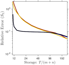
(a) LowRankHiNoise

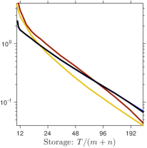
(b) LowRankMedNoise

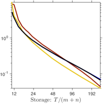
(c) LowRankLowNoise

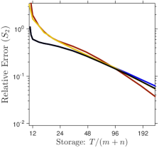
(d) PolyDecaySlow

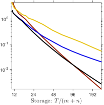
(e) PolyDecayMed

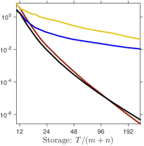
(f) PolyDecayFast

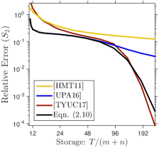
(g) ExpDecaySlow

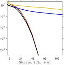
(h) ExpDecayMed

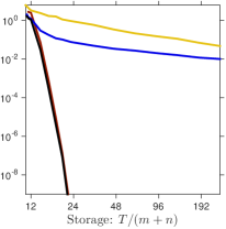
(i) ExpDecayFast

Figure 1: Comparison of reconstruction formulas: Synthetic examples. (Gaussian maps, effective rank $R=10$, approximation rank $r=10$, Schatten 2-norm.) We compare the oracle error achieved by the proposed fixed-rank approximation Eq. 12 against methods [HMT11], [Upa16], and [TYUC17] from the literature. See Section 7.2.2 for details.

7.6 Comparison of Reconstruction Formulas: Synthetic Examples

Let us now compare the proposed rank-$r$ reconstruction formula Eq. 12 with [HMT11], [Upa16], and [TYUC17] on synthetic data.

Figure 1 present the results of the following experiment. For synthetic matrices with effective rank $R=10$ and truncation rank $r=10$, we compare the relative error Eq. 32 achieved by each of the four algorithms as a function of storage. We use Gaussian dimension reduction maps in these experiments; similar results are evident for other types of maps. Results for effective rank $R\in\{5,20\}$ and Schatten $\infty$-norm appear in Section D.5. Let us make some remarks:

• This experiment demonstrates clearly that the proposed approximation Eq. 12 improves over the earlier methods for most of the synthetic input matrices, almost uniformly and sometimes by orders of magnitude.

• For input matrices where the spectral tail decays slowly (PolyDecaySlow, LowRankLowNoise, LowRankMedNoise, LowRankHiNoise), the newly proposed method Eq. 12 has identical behavior to [Upa16]. The new method is slightly worse than [HMT11] in several of these cases.

• For input matrices whose spectral tail decays more quickly (ExpDecaySlow, ExpDecayMed, ExpDecayFast, PolyDecayMed, PolyDecayFast), the proposed method improves dramatically over [HMT11] and [Upa16].

• The new method Eq. 12 shows its strength over [TYUC17] when the storage budget is small. It also yields superior performance in Schatten $\infty$-norm. These differences are most evident for matrices with slow spectral decay.

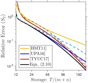
(a) MinTemp ($r=10$)

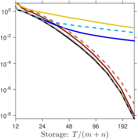
(b) StreamVel ($r=10$)

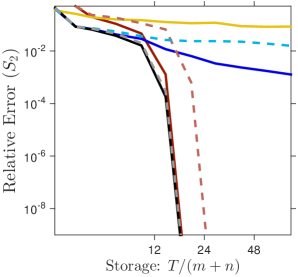
(c) MaxCut ($r=1$)

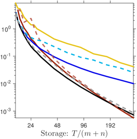
(d) MaxCut ($r=14$)

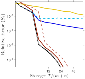
(e) PhaseRetrieval ($r=1$)

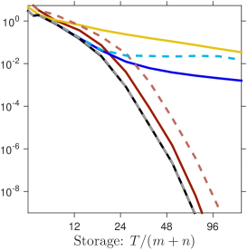
(f) PhaseRetrieval ($r=5$)

Figure 2: Comparison of reconstruction formulas: Real data examples. (Sparse maps, Schatten $2$-norm.) We compare the relative error achieved by the proposed fixed-rank approximation Eq. 12 against methods [HMT11], [Upa16], and [TYUC17] from the literature. Solid lines are oracle errors; dashed lines are errors with “natural” parameter choices. (There is no dashed line for [HMT11].) See Section 7.7 for details.

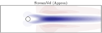
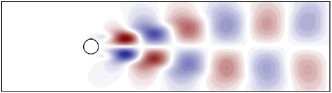
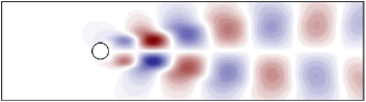
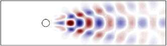
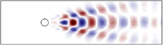
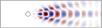
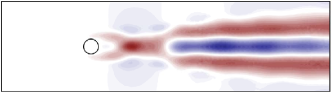
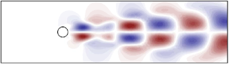
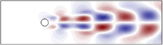
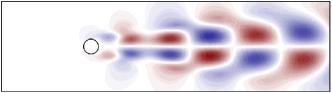
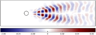
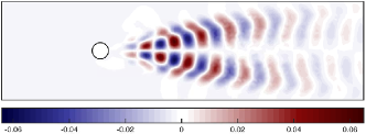
Figure 3: Left singular vectors of StreamVel. (Sparse maps, approximation rank $r=10$, storage budget $T=48(m+n)$.) The columns of the matrix StreamVel describe the fluctuations of the streamwise velocity field about its mean value as a function of time. From top to bottom, the panels show the first nine computed left singular vectors of the matrix. The left-hand side is computed from the sketch, while the right-hand side is computed from the exact flow field. The heatmap indicates the magnitude of the fluctuation. See Section 7.8 for details.

7.7 Comparison of Reconstruction Formulas: Real Data Examples

The next set of experiments compares the behavior of the algorithms for matrices drawn from applications.

Figure 2 contains the results of the following experiment. For each of the four algorithms, we display the relative error Eq. 32 as a function of storage. We use sparse dimension reduction maps, which is justified by the experiments in Section 7.4.

We plot the oracle error (Section 7.2.2) attained by each method. Since the oracle error is not achievable in practice, we also chart the performance of each method at an a priori parameter selection; see Section D.6 for details.

As with the synthetic examples, the proposed method Eq. 12 improves over the competing methods for all the examples we considered. This is true when we compare oracle errors or when we compare the errors using theoretical parameter choices. The benefits of the new method are least pronounced for the matrix MinTemp, whose spectrum has medium polynomial decay. The benefits of the new method are quite clear for the matrix StreamVel, which has an exponentially decaying spectrum. The advantages are even more striking for the two matrices MaxCut and PhaseRetrieval, which are effectively rank deficient.

In summary, we believe that the numerical work here supports the use of our new method Eq. 12. The methods [HMT11] and [Upa16] cannot achieve a small relative error Eq. 32, even with a large amount of storage. The method [TYUC17] can yield small relative error, but it often requires more storage to achieve this goal—especially at the a priori parameter choices.

7.8 Example: Flow-Field Reconstruction

Next, we elaborate on using sketching to compress the Navier–Stokes data matrix StreamVel. We compute the best rank-$10$ approximation of the matrix via Eq. 12 using storage $T=48(m+n)$ and the “natural” parameter choices Eq. 20. For this example, we can use plots of the flow field to make visual comparisons.

Fig. 3 illustrates the leading left singular vectors of the streamwise velocity field StreamVel, as computed from the sketch and the full matrix. We see that the approximate left singular vectors closely match the actual left singular vectors, although some small discrepancies appear in the higher singular vectors. See Section D.7 for additional numerics. In particular, we find that the output from the algorithms [HMT11] and [Upa16] changes violently when we adjust the truncation rank $r$.

We see that our sketching method leads to an excellent rank-$10$ approximation of the matrix. In fact, the relative error (32) in Frobenius norm is under $9.2\cdot 10^{-3}$. While the sketch uses $5.8\,\mathrm{MB}$ of storage in double precision, the full matrix requires $409.7\,\mathrm{MB}$. The compression rate is $70.6\times$. Therefore, it is possible to compress the output of the Navier–Stokes simulation automatically using sketching.

7.9 Rank Truncation and A Posteriori Error Estimation

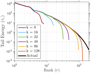
(a) Tail Energy $\tau_{r}(\hat{\bm{A}})$

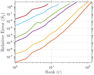
(b) Rank-$r$ Truncations

Figure 4: Why Truncate? (StreamVel, sparse maps, $s=2k+1$.) Figure 4(a) compares the tail energy $\tau_{r}(\hat{\bm{A}})$ of the rank-$k$ approximation $\hat{\bm{A}}$ against the tail energy $\tau_{r}(\bm{A})$ of the actual matrix $\bm{A}$. Figure 4(b) shows the relative error Eq. 32 in the truncated approximation $\llbracket{\hat{\bm{A}}}\rrbracket_{r}$ as a function of rank $r$. The relative error in the rank-$k$ approximation (right endpoints of series) increases with $k$. See Section 7.9.

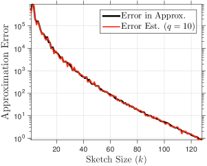
(a) Error Estimates for $\hat{\bm{A}}$

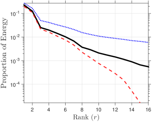
(b) Scree Plot ($k=16$)

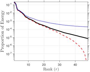
(c) Scree Plot ($k=48$)

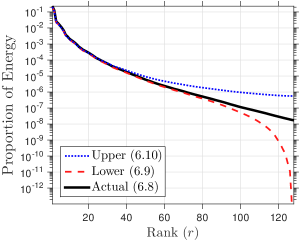
(d) Scree Plot ($k=128$)

Figure 5: Error Estimation and Scree Plots. (StreamVel, sparse maps, $s=2k+1$.) For an error sketch with size $q=10$, Fig. 5(a) compares the absolute error $\|\bm{A}-\hat{\bm{A}}\|_{2}^{2}$ in the rank-$k$ approximation versus the estimate $\mathrm{err}_{2}^{2}(\hat{\bm{A}})$. The other panels are scree plots of the actual proportion of energy remaining Eq. 29 versus a computable lower estimate Eq. 30 and upper estimate Eq. 31. See Section 7.9.

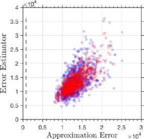
(a) Rank-$k$ Approximation ($k=16$)

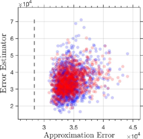
(b) Rank-$r$ Truncation ($k=16$, $r=4$)

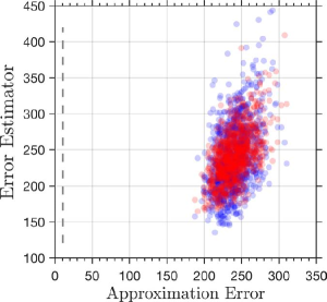
(c) Rank-$k$ Approximation ($k=48$)

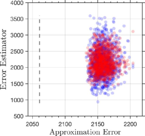
(d) Rank-$r$ Truncation ($k=48$, $r=12$)

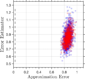
(e) Rank-$k$ Approximation ($k=128$)

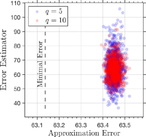
(f) Rank-$r$ Truncation ($k=128$, $r=32$)

Figure 6: Sampling Distributions of the Approximation Error and the Error Estimator. (StreamVel, sparse maps, $s=2k+1$, Schatten $2$-norm.) For error sketches with size $q\in\{5,10\}$, the left-hand side shows the sampling distribution of the error $\|\bm{A}-\hat{\bm{A}}\|_{2}^{2}$ in the rank-$k$ approximation versus the sampling distribution of the error estimator $\mathrm{err}_{2}^{2}(\hat{\bm{A}})$ for several values of $k$. The dashed line marks the error in the best rank-$k$ approximation of $\bm{A}$. The right-hand side contains similar plots with $\hat{\bm{A}}$ replaced by the rank-$r$ truncation $\llbracket{\hat{\bm{A}}}\rrbracket_{r}$. See Section 7.9.

This section uses the Navier–Stokes data to explore the behavior of the error estimator Section 6.2. We also demonstrate that it is important to truncate the rank of the approximation, and we show that the error estimator can assist us.

Let us undertake a single trial of the following experiment with the matrix StreamVel. For each sketch size parameter $k\in\{1,2,\dots,128\}$, set the other sketch size parameter $s=2k+1$. Extract an error sketch with size $q=10$. In each instance, we use the formula Eq. 11 to construct an initial rank-$k$ approximation $\hat{\bm{A}}$ of the data matrix $\bm{A}$ and the formula Eq. 12 to construct a truncated rank-$r$ approximation $\llbracket{\hat{\bm{A}}}\rrbracket_{r}$. The plots will be indexed with the sketch size parameter $k$ or the rank truncation parameter $r$, rather than the storage budget.

Figure 4 illustrates the need to truncate the rank of the approximation. Observe that the tail energy $\tau_{r}(\hat{\bm{A}})$ of the rank-$k$ approximation significantly underestimates the tail energy $\tau_{r}(\bm{A})$ of the matrix when $r\approx k$. As a consequence, the error Eq. 32 in the rank-$k$ approximation $\hat{\bm{A}}$, relative to the best rank-$k$ approximation of $\bm{A}$, actually increases with $k$. In contrast, when $r\ll k$, the rank-$r$ truncation $\llbracket{\hat{\bm{A}}}\rrbracket_{r}$ can attain very small error, relative to the best rank-$r$ approximation of $\bm{A}$. In this instance, we achieve relative error below $10^{-2}$ across a range of parameters $k$ by selecting $r\leq k/4$. Therefore, we can be confident about the quality of our estimates for the first $r$ singular vectors of $\bm{A}$.

Next, let us study the behavior of the error estimator Eq. 25. Figure 5 compares the actual approximation error $\|\bm{A}-\hat{\bm{A}}\|_{2}^{2}$ and the empirical error estimate $\mathrm{err}_{2}^{2}(\hat{\bm{A}})$ as a function of the sketch size $k$. The other panels are scree plots. The baseline is the actual scree function Eq. 29 computed from the input matrix. The remaining curves are the lower Eq. 30 and upper Eq. 31 estimates for this curve. We see that the scree estimators give good lower and upper bounds for the energy missed, while tracking the shape of the baseline curve. As a consequence, we can use these empirical estimates to select the truncation rank.

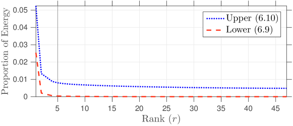
Figure 7: Empirical Scree Plot for SeaSurfaceTemp Approximation. (Sparse maps, $k=48$, $s=839$, $q=10$.) The lower Eq. 30 and upper Eq. 31 approximations of the scree curve Eq. 29. The vertical line marks the truncation rank $r=5$. See Sections 7.10 and 1 for details.

Table 1: A Posteriori Error Evaluation of Sea Surface Temperature Approximations. This table lists the lower and upper estimates for the true scree curve Eq. 29 of the matrix SeaSurfaceTemp. We truncate at rank $r=5$ (blue).

Rank	Lower Estimate Eq. 30	Upper Estimate Eq. 31
($r$)	$\underline{\mathrm{scree}}(r)$	$\overline{\mathrm{scree}}(r)$
1	$2.5415\cdot 10^{-2}$	$5.2454\cdot 10^{-2}$
2	$2.1068\cdot 10^{-3}$	$1.3342\cdot 10^{-2}$
3	$1.2867\cdot 10^{-3}$	$1.1126\cdot 10^{-2}$
4	$5.8939\cdot 10^{-4}$	$8.8143\cdot 10^{-3}$
5	$3.9590\cdot 10^{-4}$	$8.0110\cdot 10^{-3}$
6	$3.0878\cdot 10^{-4}$	$7.6002\cdot 10^{-3}$
7	$2.5140\cdot 10^{-4}$	$7.3039\cdot 10^{-3}$
8	$2.1541\cdot 10^{-4}$	$7.1038\cdot 10^{-3}$
9	$1.8673\cdot 10^{-4}$	$6.9342\cdot 10^{-3}$
10	$1.6410\cdot 10^{-4}$	$6.7926\cdot 10^{-3}$

Last, we investigate the sampling distribution of the error in the randomized matrix approximation and the sampling distribution of the error estimator. To do so, we perform 1000 independent trials of the same experiment for select values of $k$ and with error sketch sizes $q\in\{5,10\}$.

Figure 6 contains scatter plots of the actual approximation error $\|\bm{A}-\hat{\bm{A}}_{\rm out}\|_{2}^{2}$ versus the estimated approximation error $\mathrm{err}_{2}^{2}(\hat{\bm{A}}_{\rm out})$ for $\hat{\bm{A}}_{\rm out}=\hat{\bm{A}}$ and $\hat{\bm{A}}_{\rm out}=\llbracket{\hat{\bm{A}}}\rrbracket_{r}$. The error estimators are unbiased, but they exhibit a lot of variability. Doubling the error sketch size $q$ reduces the spread of the error estimate by a factor of two. The approximation errors cluster tightly, as we expect from concentration of measure. The plots also highlight that the initial rank-$k$ approximations are far from attaining the minimal rank-$k$ error, while the truncated rank-$r$ approximations are more successful.

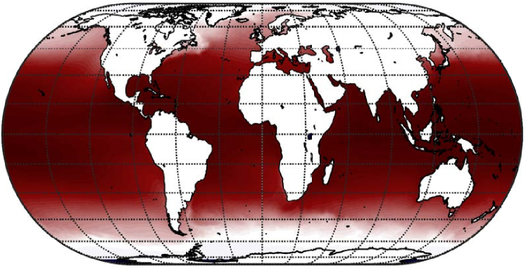
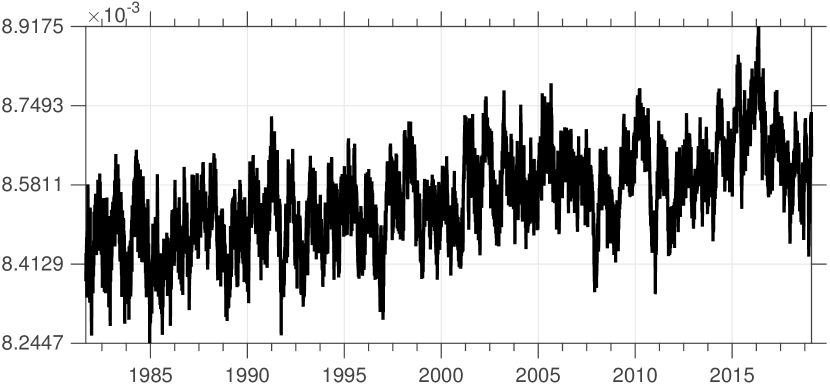
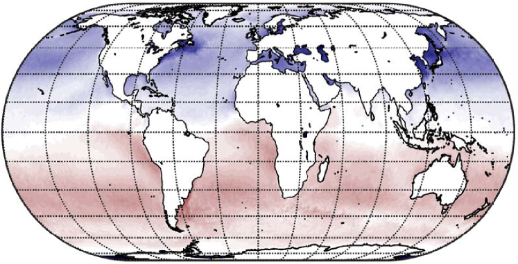
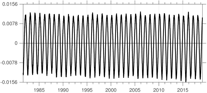
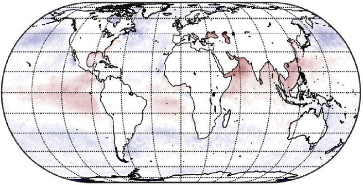
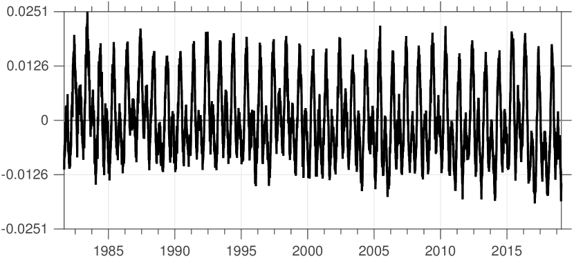
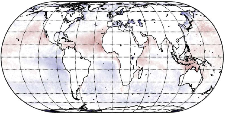
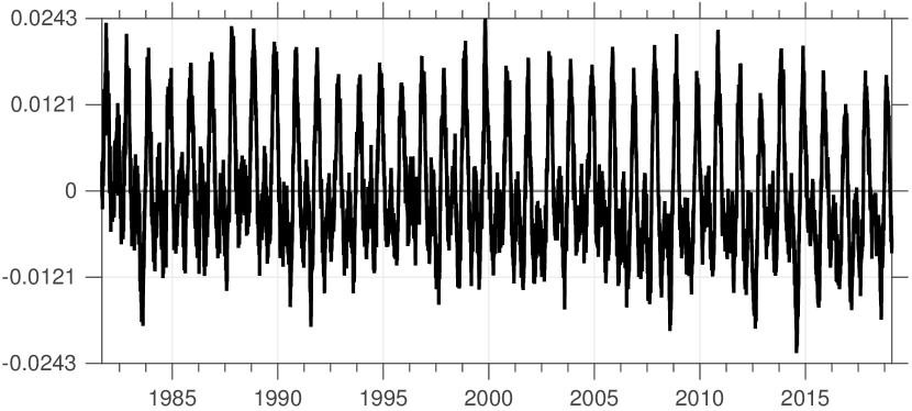
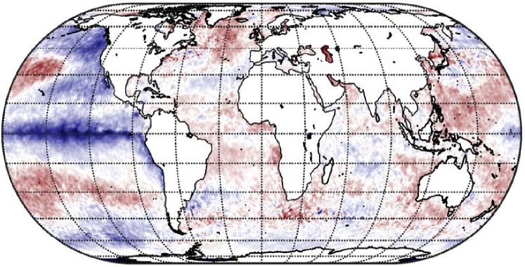
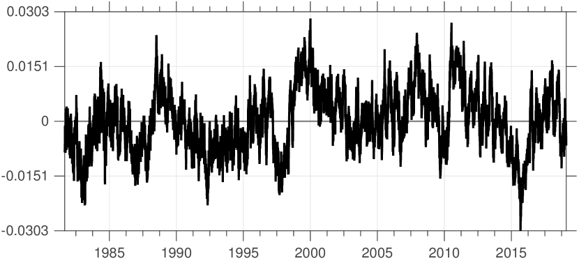
Figure 8: Singular Vectors of SeaSurfaceTemp. (Sparse maps, $k=48$, $s=839$, $q=10$.) The left column displays the first five left singular vectors. The heatmaps use white to represent zero Celsius degrees; each image is scaled independently. The right column displays the first five right singular vectors. The horizontal axis marks the year (common era); the vertical axis is unitless. See Section 7.10.

7.10 Example: Sea Surface Temperature Data

Finally, we give a complete demonstration of the overall methodology for the matrix SeaSurfaceTemp. Like the matrix MinTemp, we expect that the sea surface temperature data has medium polynomial decay, so it should be well approximated by a low-rank matrix.

1. Parameter selection. We fix the storage budget $T=48(m+n)$. The natural parameter selection Eq. 20 yields $k=47$ and $s=839$. We use sparse dimension reduction maps. The error sketch has size $q=10$.

2. Data collection. We “stream” the data one year at a time to construct the approximation and error sketches.

3. Error estimates and rank truncation. Once the data is collected, we compute the rank-$k$ approximation $\hat{\bm{A}}$ using the formula Eq. 11. We present the empirical scree estimates Eqs. 30 and 31 in Figs. 7 and 1. These values should bracket the unknown scree curve Eq. 29, while mimicking its shape. By visual inspection, we set the truncation rank $r=5$. We expect that the rank-$5$ approximation captures all but $0.04\%$ to $0.8\%$ of the energy.

4. Visualization. Figure 8 illustrates the first five singular vector pairs of the rank-$r$ approximation of the matrix SeaSurfaceTemp. The first left singular vector can be interpreted as the mean temperature profile; a warming trend is visible in the first right singular vector. The second pair reflects the austral/boreal divide. The remaining singular vectors capture long-term climatological features.

The total storage required for the approximation sketch and the error sketch is $4.09\cdot 10^{7}$ numbers. This stands in contrast to the $mn=9.09\cdot 10^{9}$ numbers appearing in the matrix itself. The compression ratio is $222\times$. Moreover, the computational time required to obtain the approximation is modest because we are working with substantially smaller matrices.

8 Conclusions

This paper exhibits a sketching method and a new reconstruction algorithm for low-rank approximation of matrices that are presented as a sequence of linear updates (Section 2). The algorithm is accompanied by a priori error bounds that allow us to set algorithm parameters reliably (Section 5), as well as an a posteriori error estimator that allows us to validate its performance and to select the final rank of the approximation (Section 6). We discuss implementation issues (Sections 3 and 4), and we present numerical experiments to show that the new method improves over existing techniques (Sections 7.6 and 7.7).

A potential application of these techniques is for on-the-fly-compression of large-scale scientific simulations and data collection. Our experiments with a Navier–Stokes simulation (Section 7.8) and with sea surface temperature data (Section 7.10) both support this hypothesis. We hope that this work motivates researchers to investigate the use of sketching in new applications.

Appendix A Analysis of the Low-Rank Approximation

This section contains the proof of Theorem 5.1, the theoretical result on the behavior of the basic low-rank approximation Eq. 11. We maintain the notation from Section 2.

A.1 Facts about Random Matrices

First, let us state a useful formula that allows us to compute some expectations involving a Gaussian random matrix. This identity is drawn from [35, Prop. A.1 and A.6]. See also [69, Fact A.1].

Fact 1.

Assume that $t>q+\alpha$. Let $\bm{G}_{1}\in\mathbb{F}^{t\times q}$ and $\bm{G}_{2}\in\mathbb{F}^{t\times p}$ be independent standard normal matrices. For any matrix $\bm{B}$ with conforming dimensions,

$$\operatorname{\mathbb{E}}\|\bm{G}_{1}^{\dagger}\bm{G}_{2}\bm{B}\|_{2}^{2}=\frac{q}{t-q-\alpha}\cdot\|\bm{B}\|_{2}^{2}.$$

The number $\alpha=1$ when $\mathbb{F}=\mathbb{R}$, while $\alpha=0$ when $\mathbb{F}=\mathbb{C}$.

A.2 Results from Randomized Linear Algebra

Our argument also depends on the analysis of randomized low-rank approximation developed in [35, Sec. 10].

Fact 2 (Halko et al. 2011).

Fix $\bm{A}\in\mathbb{F}^{m\times n}$. Let $\varrho$ be a natural number such that $\varrho<k-\alpha$. Draw the random test matrix $\bm{\Omega}\in\mathbb{F}^{k\times n}$ from the standard normal distribution. Then the matrix $\bm{Q}\in\mathbb{F}^{m\times k}$ computed by Eq. 9 satisfies

$$\operatorname{\mathbb{E}}_{\bm{\Omega}}\|\bm{A}-\bm{QQ}^{*}\bm{A}\|_{2}^{2}\leq\left(1+\frac{\varrho}{k-\varrho-\alpha}\right)\cdot\tau_{\varrho+1}^{2}(\bm{A}).$$

An analogous result holds for the matrix $\bm{P}\in\mathbb{F}^{n\times k}$ computed by Eq. 9:

$$\operatorname{\mathbb{E}}_{\bm{\Upsilon}}\|\bm{A}-\bm{A}\bm{PP}^{*}\|_{2}^{2}\leq\left(1+\frac{\varrho}{k-\varrho-\alpha}\right)\cdot\tau_{\varrho+1}^{2}(\bm{A}).$$

The number $\alpha=1$ when $\mathbb{F}=\mathbb{R}$, while $\alpha=0$ when $\mathbb{F}=\mathbb{C}$.

This result follows immediately from the proof of [35, Thm. 10.5] using Fact 1 to handle both the real and complex case simultaneously. See also [70, Sec. 8.2].

A.3 Decomposition of the Core Matrix Approximation Error

The first step in the argument is to obtain a formula for the error in the approximation $\bm{C}-\bm{Q}^{*}\bm{A}\bm{P}$. The core matrix $\bm{C}\in\mathbb{F}^{s\times s}$ is defined in (10). We constructed the orthonormal matrices $\bm{P}\in\mathbb{F}^{n\times k}$ and $\bm{Q}\in\mathbb{F}^{m\times k}$ in (9).

Let us introduce matrices whose ranges are complementary to those of $\bm{P}$ and $\bm{Q}$:

$$\bm{P}_{\perp}\bm{P}_{\perp}^{*}:=\mathbf{I}-\bm{PP}^{*} \quad\text{where}\quad\bm{P}_{\perp}\in\mathbb{F}^{n\times(n-k)};$$

$$\bm{Q}_{\perp}\bm{Q}_{\perp}^{*}:=\mathbf{I}-\bm{QQ}^{*} \quad\text{where}\quad\bm{Q}_{\perp}\in\mathbb{F}^{m\times(m-k)}.$$

The columns of $\bm{P}_{\perp}$ are orthonormal, and the columns of $\bm{Q}_{\perp}$ are orthonormal. Next, introduce the submatrices

(33) $$\bm{\Phi}_{1}=\bm{\Phi}\bm{Q}\in\mathbb{F}^{s\times k} \quad\text{and}\quad\bm{\Phi}_{2}=\bm{\Phi}\bm{Q}_{\perp}\in\mathbb{F}^{s\times(m-k)};$$

$$\bm{\Psi}_{1}^{*}=\bm{P}^{*}\bm{\Psi}^{*}\in\mathbb{F}^{k\times s} \quad\text{and}\quad\bm{\Psi}_{2}^{*}=\bm{P}_{\perp}^{*}\bm{\Psi}^{*}\in\mathbb{F}^{(n-k)\times s}.$$

With this notation at hand, we can state and prove the first result.

Lemma A.1 (Decomposition of the Core Matrix Approximation).

Assume that the matrices $\bm{\Phi}_{1}$ and $\bm{\Psi}_{1}$ have full column rank. Then

$$\bm{C}-\bm{Q}^{*}\bm{A}\bm{P} =\bm{\Phi}_{1}^{\dagger}\bm{\Phi}_{2}(\bm{Q}_{\perp}^{*}\bm{A}\bm{P})+(\bm{Q}^{*}\bm{A}\bm{P}_{\perp})\bm{\Psi}_{2}^{*}(\bm{\Psi}_{1}^{\dagger})^{*}$$

$$+\bm{\Phi}_{1}^{\dagger}\bm{\Phi}_{2}(\bm{Q}_{\perp}^{*}\bm{A}\bm{P}_{\perp})\bm{\Psi}_{2}^{*}(\bm{\Psi}_{1}^{\dagger})^{*}.$$

Proof A.2.

Adding and subtracting terms, we write the core sketch $\bm{Z}$ as

$$\bm{Z}=\bm{\Phi}\bm{A}\bm{\Psi}^{*}=\bm{\Phi}(\bm{A}-\bm{QQ}^{*}\bm{A}\bm{PP}^{*})\bm{\Psi}^{*}+(\bm{\Phi Q})(\bm{Q}^{*}\bm{A}\bm{P})(\bm{P}^{*}\bm{\Psi}^{*}).$$

Using (33), we identify the matrices $\bm{\Phi}_{1}$ and $\bm{\Psi}_{1}$. Then left-multiply by $\bm{\Phi}_{1}^{\dagger}$ and right-multiply by $(\bm{\Psi}_{1}^{\dagger})^{*}$ to arrive at

$$\bm{C}=\bm{\Phi}_{1}^{\dagger}\bm{Z}(\bm{\Psi}_{1}^{\dagger})^{*}=\bm{\Phi}_{1}^{\dagger}\bm{\Phi}(\bm{A}-\bm{QQ}^{*}\bm{A}\bm{PP}^{*})\bm{\Psi}^{*}(\bm{\Psi}_{1}^{\dagger})^{*}+\bm{Q}^{*}\bm{A}\bm{P}.$$

We have identified the core matrix $\bm{C}$, defined in Eq. 10. Move the term $\bm{Q}^{*}\bm{A}\bm{P}$ to the left-hand side to isolate the approximation error.

To continue, notice that

$$\bm{\Phi}_{1}^{\dagger}\bm{\Phi}=\bm{\Phi}_{1}^{\dagger}\bm{\Phi}\bm{QQ}^{*}+\bm{\Phi}_{1}^{\dagger}\bm{\Phi}\bm{Q}_{\perp}\bm{Q}_{\perp}^{*}=\bm{Q}^{*}+\bm{\Phi}_{1}^{\dagger}\bm{\Phi}_{2}\bm{Q}_{\perp}^{*}.$$

Likewise,

$$\bm{\Psi}^{*}(\bm{\Psi}_{1}^{\dagger})^{*}=\bm{PP}^{*}\bm{\Psi}^{*}(\bm{\Psi}_{1}^{\dagger})^{*}+\bm{P}_{\perp}\bm{P}_{\perp}^{*}\bm{\Psi}^{*}(\bm{\Psi}_{1}^{\dagger})^{*}=\bm{P}+\bm{P}_{\perp}\bm{\Psi}_{2}^{*}(\bm{\Psi}_{1}^{\dagger})^{*}.$$

Combine the last three displays to arrive at

$$\bm{C}-\bm{Q}^{*}\bm{A}\bm{P}=(\bm{Q}^{*}+\bm{\Phi}_{1}^{\dagger}\bm{\Phi}_{2}\bm{Q}_{\perp}^{*})(\bm{A}-\bm{QQ}^{*}\bm{A}\bm{PP}^{*})(\bm{P}+\bm{P}_{\perp}\bm{\Psi}_{2}^{*}(\bm{\Psi}_{1}^{\dagger})^{*}).$$

Expand the expression and use the orthogonality relations $\bm{Q}^{*}\bm{Q}=\mathbf{I}$ and $\bm{Q}_{\perp}^{*}\bm{Q}=\bm{0}$ and $\bm{P}^{*}\bm{P}=\mathbf{I}$ and $\bm{P}^{*}\bm{P}_{\perp}=\bm{0}$ to arrive at the desired representation.

A.4 Probabilistic Analysis of the Core Matrix

Next, we make distributional assumptions on the dimension reduction maps $\bm{\Phi}$ and $\bm{\Psi}$. We can then study the probabilistic behavior of the error $\bm{C}-\bm{Q}^{*}\bm{A}\bm{P}$, conditional on $\bm{Q}$ and $\bm{P}$.

Lemma A.3 (Probabilistic Analysis of the Core Matrix).

Assume that the dimension reduction matrices $\bm{\Phi}$ and $\bm{\Psi}$ are drawn independently from the standard normal distribution. When $s\geq k$, it holds that

(34) $$\operatorname{\mathbb{E}}_{\bm{\Phi},\bm{\Psi}}[\bm{C}-\bm{Q}^{*}\bm{A}\bm{P}]=\bm{0}.$$

When $s>k+\alpha$, we can express the error as

$$\operatorname{\mathbb{E}}_{\bm{\Phi},\bm{\Psi}}\|\bm{C}-\bm{Q}^{*}\bm{A}\bm{P}\|_{2}^{2} =\frac{k}{s-k-\alpha}\cdot\|\bm{A}-\bm{QQ}^{*}\bm{A}\bm{PP}^{*}\|_{2}^{2}$$

$$\qquad+\frac{k(2k+\alpha-s)}{(s-k-\alpha)^{2}}\cdot\|\bm{Q}_{\perp}^{*}\bm{A}\bm{P}_{\perp}\|_{2}^{2}.$$

When $s<2k+\alpha$, the last term is nonnegative; when $s\geq 2k+\alpha$, the last term is nonpositive.

Proof A.4.

Since $\bm{\Phi}$ is standard normal, the orthogonal submatrices $\bm{\Phi}_{1}$ and $\bm{\Phi}_{2}$ are statistically independent standard normal matrices because of the marginal property of the normal distribution. Likewise, $\bm{\Psi}_{1}$ and $\bm{\Psi}_{2}$ are statistically independent standard normal matrices. Provided that $s\geq k$, both matrices have full column rank with probability one.

To establish the formula (34), notice that

$$\operatorname{\mathbb{E}}_{\bm{\Phi},\bm{\Psi}}[\bm{C}-\bm{Q}^{*}\bm{A}\bm{P}] =\operatorname{\mathbb{E}}_{\bm{\Phi}_{1}}\operatorname{\mathbb{E}}_{\bm{\Phi}_{2}}[\bm{\Phi}_{1}^{\dagger}\bm{\Phi}_{2}(\bm{Q}_{\perp}^{*}\bm{A}\bm{P})]+\operatorname{\mathbb{E}}_{\bm{\Psi}_{1}}\operatorname{\mathbb{E}}_{\bm{\Psi}_{2}}[(\bm{Q}^{*}\bm{A}\bm{P}_{\perp})\bm{\Psi}_{2}^{*}(\bm{\Psi}_{1}^{\dagger})^{*}]$$

$$+\operatorname{\mathbb{E}}\operatorname{\mathbb{E}}_{\bm{\Phi}_{2}}[\bm{\Phi}_{1}^{\dagger}\bm{\Phi}_{2}(\bm{Q}_{\perp}^{*}\bm{A}\bm{P}_{\perp})\bm{\Psi}_{2}^{*}(\bm{\Psi}_{1}^{\dagger})^{*}].$$

We have used the decomposition of the approximation error from Lemma A.1. Then we invoke independence to write the expectations as iterated expectations. Since $\bm{\Phi}_{2}$ and $\bm{\Psi}_{2}$ have mean zero, this formula makes it clear that the approximation error has mean zero.

To study the fluctuations, apply the independence and zero-mean property of $\bm{\Phi}_{2}$ and $\bm{\Psi}_{2}$ to decompose

$$\operatorname{\mathbb{E}}_{\bm{\Phi},\bm{\Psi}}\|\bm{C}-\bm{Q}^{*}\bm{A}\bm{P}\|_{2}^{2} =\operatorname{\mathbb{E}}_{\bm{\Phi}}\|\bm{\Phi}_{1}^{\dagger}\bm{\Phi}_{2}(\bm{Q}_{\perp}^{*}\bm{A}\bm{P})\|_{2}^{2}+\operatorname{\mathbb{E}}_{\bm{\Psi}}\|(\bm{Q}^{*}\bm{A}\bm{P}_{\perp})\bm{\Psi}_{2}^{*}(\bm{\Psi}_{1}^{\dagger})^{*}\|_{2}^{2}$$

$$+\operatorname{\mathbb{E}}_{\bm{\Phi}}\operatorname{\mathbb{E}}_{\bm{\Psi}}\|\bm{\Phi}_{1}^{\dagger}\bm{\Phi}_{2}(\bm{Q}_{\perp}^{*}\bm{A}\bm{P}_{\perp})\bm{\Psi}_{2}^{*}(\bm{\Psi}_{1}^{\dagger})^{*}\|_{2}^{2}.$$

Continuing, we invoke Fact 1 four times to see that

$$\operatorname{\mathbb{E}}_{\bm{\Phi},\bm{\Psi}}\|\bm{C}-\bm{Q}^{*}\bm{A}\bm{P}\|_{2}^{2}\\ =\frac{k}{s-k-\alpha}\cdot\left[\|\bm{Q}_{\perp}^{*}\bm{A}\bm{P}\|_{2}^{2}+\|\bm{Q}^{*}\bm{A}\bm{P}_{\perp}\|_{2}^{2}+\frac{k}{s-k-\alpha}\cdot\|\bm{Q}_{\perp}^{*}\bm{A}\bm{P}_{\perp}\|_{2}^{2}\right].$$

Add and subtract $\|\bm{Q}_{\perp}^{*}\bm{A}\bm{P}_{\perp}\|_{2}^{2}$ in the bracket to arrive at

$$\operatorname{\mathbb{E}}\|\bm{C}-\bm{Q}^{*}\bm{A}\bm{P}\|_{2}^{2} =\frac{k}{s-k-\alpha}\cdot\bigg{[}\|\bm{Q}_{\perp}^{*}\bm{A}\bm{P}\|_{2}^{2}+\|\bm{Q}^{*}\bm{A}\bm{P}_{\perp}\|_{2}^{2}+\|\bm{Q}_{\perp}^{*}\bm{A}\bm{P}_{\perp}\|_{2}^{2}$$

$$\qquad+\frac{2k+\alpha-s}{s-k-\alpha}\cdot\|\bm{Q}_{\perp}^{*}\bm{A}\bm{P}_{\perp}\|_{2}^{2}\bigg{]}.$$

Use the Pythagorean Theorem to combine the terms on the first line.

A.5 Probabilistic Analysis of the Compression Error

Next, we establish a bound for the expected error in the compression of the matrix $\bm{A}$ onto the range of the orthonormal matrices $\bm{Q}$ and $\bm{P}$, computed in Eq. 9. This result is similar in spirit to the analysis in [35], so we pass lightly over the details.

Lemma A.5 (Probabilistic Analysis of the Compression Error).

For any natural number $\varrho<k-\alpha$, it holds that

$$\operatorname{\mathbb{E}}\|\bm{A}-\bm{QQ}^{*}\bm{A}\bm{PP}^{*}\|_{2}^{2}\leq\left(1+\frac{2\varrho}{k-\varrho-\alpha}\right)\cdot\tau_{\varrho+1}^{2}(\bm{A}).$$

Proof A.6 (Proof Sketch).

Introduce the partitioned SVD of the matrix $\bm{A}$:

$$\bm{A}=\bm{U\Sigma V}^{*}=\begin{bmatrix}\bm{U}_{1}&\bm{U}_{2}\end{bmatrix}\begin{bmatrix}\bm{\Sigma}_{1}&\\ &\bm{\Sigma}_{2}\end{bmatrix}\begin{bmatrix}\bm{V}_{1}^{*}\\ \bm{V}_{2}^{*}\end{bmatrix}\quad\text{where}\quad\bm{\Sigma}_{1}\in\mathbb{F}^{\varrho\times\varrho}.$$

Define the matrices

$$\bm{\Upsilon}_{1}:=\bm{\Upsilon}\bm{U}_{1}\in\mathbb{F}^{s\times\varrho}\quad\text{and}\quad\bm{\Upsilon}_{2}:=\bm{\Upsilon}\bm{U}_{2}\in F^{s\times(m-\varrho)};$$

$$\bm{\Omega}_{1}^{*}:=\bm{V}_{1}^{*}\bm{\Omega}^{*}\in\mathbb{F}^{\varrho\times s}\quad\text{and}\quad\bm{\Omega}_{2}^{*}:=\bm{V}_{2}^{*}\bm{\Omega}^{*}\in\mathbb{F}^{(n-\varrho)\times s};$$

$$\bm{P}_{1}:=\bm{V}_{1}^{*}\bm{P}\in\mathbb{F}^{\varrho\times k}\quad\text{and}\quad\bm{P}_{2}:=\bm{V}_{2}^{*}\bm{P}\in\mathbb{F}^{(n-\varrho)\times k}.$$

With this notation, we proceed to the proof.

First, add and subtract terms and apply the Pythagorean Theorem to obtain

$$\|\bm{A}-\bm{QQ}^{*}\bm{A}\bm{PP}^{*}\|_{2}^{2}=\|\bm{A}(\mathbf{I}-\bm{PP}^{*})\|_{2}^{2}+\|(\mathbf{I}-\bm{QQ}^{*})\bm{A}\bm{PP}^{*}\|_{2}^{2}.$$

Use the SVD to decompose the matrix $\bm{A}$ in the first term, and apply the Pythagorean Theorem again:

$$\|\bm{A}-\bm{QQ}^{*}\bm{A}\bm{PP}^{*}\|_{2}^{2}=\|(\bm{U}_{2}\bm{\Sigma}_{2}\bm{V}_{2}^{*})(\mathbf{I}-\bm{PP}^{*})\|_{2}^{2}\\ +\|(\bm{U}_{1}\bm{\Sigma}_{1}\bm{V}_{1}^{*})(\mathbf{I}-\bm{PP}^{*})\|_{2}^{2}+\|(\mathbf{I}-\bm{QQ}^{*})\bm{A}\bm{P}\|_{2}^{2}.$$

The result [70, Prop. 9.2] implies that the second term satisfies

$$\|(\bm{U}_{1}\bm{\Sigma}_{1}\bm{V}_{1}^{*})(\mathbf{I}-\bm{PP}^{*})\|_{2}^{2}\leq\|\bm{\Upsilon}_{1}^{\dagger}\bm{\Upsilon}_{2}\bm{\Sigma}_{2}\|_{2}^{2}.$$

We can obtain a bound for the third term using the formula [35, p. 270, disp. 1]. After a short computation, this result yields

$$\|(\mathbf{I}-\bm{QQ}^{*})\bm{AP}\|_{2}^{2} \leq\|\bm{\Sigma}_{2}\bm{P}_{2}\|_{2}^{2}+\|\bm{\Sigma}_{2}\bm{\Omega}_{2}^{*}(\bm{\Omega}_{1}^{*})^{\dagger}\bm{P}_{1}\|_{2}^{2}$$

$$\leq\|\bm{\Sigma}_{2}\|_{2}^{2}+\|\bm{\Sigma}_{2}\bm{\Omega}_{2}^{*}(\bm{\Omega}_{1}^{*})^{\dagger}\|_{2}^{2}.$$

We can remove $\bm{P}_{1}$ and $\bm{P}_{2}$ because their spectral norms are bounded by one, being submatrices of the orthonormal matrix $\bm{P}$. Combine the last three displays to obtain

$$\|\bm{A}-\bm{QQ}^{*}\bm{A}\bm{PP}^{*}\|_{2}^{2}\leq\|\bm{\Sigma}_{2}\|_{2}^{2}+\|\bm{\Upsilon}_{1}^{\dagger}\bm{\Upsilon}_{2}\bm{\Sigma}_{2}\|_{2}^{2}+\|\bm{\Sigma}_{2}\bm{\Omega}_{2}^{*}(\bm{\Omega}_{1}^{*})^{\dagger}\|_{2}^{2}.$$

We have used the Pythagorean Theorem again.

Take the expectation with respect to $\bm{\Upsilon}$ and $\bm{\Omega}$ to arrive at

$$\operatorname{\mathbb{E}}\|\bm{A}-\bm{QQ}^{*}\bm{A}\bm{PP}^{*}\|_{2}^{2} \leq\|\bm{\Sigma}_{2}\|_{2}^{2}+\operatorname{\mathbb{E}}\|\bm{\Upsilon}_{1}^{\dagger}\bm{\Upsilon}_{2}\bm{\Sigma}_{2}\|_{2}^{2}+\operatorname{\mathbb{E}}\|\bm{\Sigma}_{2}\bm{\Omega}_{2}^{*}(\bm{\Omega}_{1}^{*})^{\dagger}\|_{2}^{2}$$

$$=\|\bm{\Sigma}_{2}\|_{2}^{2}+\frac{2\varrho}{k-\varrho-\alpha}\cdot\|\bm{\Sigma}_{2}\|_{2}^{2}.$$

Finally, note that $\|\bm{\Sigma}_{2}\|_{2}^{2}=\tau_{\varrho+1}^{2}(\bm{A})$.

A.6 The Endgame

At last, we are prepared to finish the proof of Theorem 5.1. Fix a natural number $\varrho<k-\alpha$. Using the formula Eq. 11 for the approximation $\hat{\bm{A}}$, we see that

$$\|\bm{A}-\hat{\bm{A}}\|_{2}^{2} =\|\bm{A}-\bm{Q}\bm{C}\bm{P}^{*}\|_{2}^{2}$$

$$=\|\bm{A}-\bm{QQ}^{*}\bm{A}\bm{PP}^{*}+\bm{Q}(\bm{Q}^{*}\bm{A}\bm{P}-\bm{C})\bm{P}^{*}\|_{2}^{2}$$

$$=\|\bm{A}-\bm{QQ}^{*}\bm{A}\bm{PP}^{*}\|_{2}^{2}+\|\bm{Q}(\bm{Q}^{*}\bm{A}\bm{P}-\bm{C})\bm{P}^{*}\|_{2}^{2}.$$

The last identity is the Pythagorean theorem. Drop the orthonormal matrices in the last term. Then take the expectation with respect to $\bm{\Phi}$ and $\bm{\Psi}$:

$$\operatorname{\mathbb{E}}_{\bm{\Phi},\bm{\Psi}}\|\bm{A}-\hat{\bm{A}}\|_{2}^{2}=\|\bm{A}-\bm{QQ}^{*}\bm{A}\bm{PP}^{*}\|_{2}^{2}+\operatorname{\mathbb{E}}_{\bm{\Phi},\bm{\Psi}}\|\bm{Q}^{*}\bm{A}\bm{P}-\bm{C}\|_{2}^{2}\\$$

We treat the two terms sequentially.

To continue, invoke the expression Lemma A.3 for the expected error in the core matrix $\bm{C}$:

$$\operatorname{\mathbb{E}}_{\bm{\Phi},\bm{\Psi}}\|\bm{A}-\hat{\bm{A}}\|_{2}^{2} \leq\left(1+\frac{k}{s-k-\alpha}\right)\cdot\|\bm{A}-\bm{QQ}^{*}\bm{A}\bm{PP}^{*}\|_{2}^{2}$$

$$+\frac{k(2k+\alpha-s)}{(s-k-\alpha)^{2}}\cdot\|\bm{Q}_{\perp}^{*}\bm{A}\bm{P}_{\perp}\|_{2}^{2}.$$

Now, take the expectation with respect to $\bm{\Upsilon}$ and $\bm{\Omega}$ to arrive at

(35) $$\operatorname{\mathbb{E}}\|\bm{A}-\hat{\bm{A}}\|_{2}^{2} \leq\left(1+\frac{k}{s-k-\alpha}\right)\cdot\left(1+\frac{2\varrho}{k-\varrho-\alpha}\right)\cdot\tau_{\varrho+1}^{2}(\bm{A})$$

$$\qquad+\frac{k(2k+\alpha-s)}{(s-k-\alpha)^{2}}\cdot\operatorname{\mathbb{E}}\|\bm{Q}_{\perp}^{*}\bm{A}\bm{P}_{\perp}\|_{2}^{2}.$$

We have invoked Lemma A.5. The last term is nonpositive because we require $s\geq 2k+\alpha$, so we may drop it from consideration. Finally, we optimize over eligible choices $\varrho<k-\alpha$ to complete the argument. The result stated in Theorem 5.1 is algebraically equivalent.

Appendix B A Posteriori Error Estimation

This section contains proofs of the bounds on the a posteriori error estimator $\mathrm{err}_{2}$ computed using a Gaussian error sketch. It also establishes the linear algebra results that we need to diagnose spectral decay in the input matrix.

B.1 The Frobenius Norm Estimator

Fix an arbitrary matrix $\bm{M}\in\mathbb{F}^{m\times n}$, which plays the role of the discrepancy $\bm{A}-\hat{\bm{A}}_{\rm out}$. For a parameter $q$, draw a standard normal dimension reduction map $\bm{\Theta}\in\mathbb{F}^{q\times m}$. Define the random variable

$$\varphi_{2}^{2}:=\frac{1}{\beta q}\cdot\|\bm{\Theta}\bm{M}\|_{2}^{2}.$$

The field parameter $\beta=1$ for $\mathbb{F}=\mathbb{R}$ and $\beta=2$ for $\mathbb{F}=\mathbb{C}$. This random variable can be regarded as a randomized estimator for the Schatten 2-norm of the matrix $\bm{M}$. The goal of this section is to develop probabilistic results to support this claim.

Remark B.1 (Prior Work).

The analysis here is similar in spirit to recent papers on randomized trace estimators [7, 61, 31]. The details here are slightly different, but we claim no novelty of insight.

B.1.1 An Alternative Representation

By the unitary invariance of the Schatten norm and the standard normal matrix, we can and will assume that $\bm{M}=\operatorname{diag}(\sigma_{1},\dots,\sigma_{m})\in\mathbb{R}^{m\times m}$ is a real diagonal matrix with (weakly) decreasing entries.

Since $\bm{M}$ is real and diagonal, the estimator can be written as

(36) $$\varphi_{2}^{2}=\frac{1}{\beta q}\cdot\|\bm{\Theta}\bm{M}\|_{2}^{2}=\frac{1}{\beta q}\cdot\sum\nolimits_{i=1}^{m}\sigma_{i}^{2}\cdot\|\bm{\theta}_{:i}\|_{2}^{2}\sim\frac{1}{\beta q}\cdot\sum\nolimits_{i=1}^{m}\sigma_{i}^{2}\chi_{i}^{2}.$$

Here, $\bm{\theta}_{:i}$ is the $i$th column of $\bm{\Theta}$. We have also introduced an independent family $\{\chi_{i}^{2}:i=1,\dots,n\}$ of chi-squared random variables, each with $\beta q$ degrees of freedom. The symbol $\sim$ denotes equality of distribution.

B.1.2 The Mean and Variance

Using the representation Eq. 36, we quickly compute the mean and variance of the estimator. By linearity of expectation,

$$\operatorname{\mathbb{E}}\varphi_{2}^{2}=\frac{1}{\beta q}\cdot\sum\nolimits_{i=1}^{m}\sigma_{i}^{2}\operatorname{\mathbb{E}}\chi_{i}^{2}=\sum\nolimits_{i=1}^{m}\sigma_{i}^{2}=\|\bm{M}\|_{2}^{2}.$$

For the second relation, we introduce the mean of a chi-squared variable with $\beta q$ degrees of freedom. Since the chi-squared variables are independent,

$$\operatorname{Var}[\varphi_{2}^{2}]=\frac{1}{(\beta q)^{2}}\cdot\sum\nolimits_{i=1}^{m}\sigma_{i}^{4}\operatorname{Var}[\chi_{i}^{2}]=\frac{2}{\beta q}\sum\nolimits_{i=1}^{m}\sigma_{i}^{4}=\frac{2}{\beta q}\|\bm{M}\|_{4}^{4}.$$

We have also used the fact that the variance is 2-homogeneous, and we introduced the variance of a chi-squared variable with $\beta q$ degrees of freedom.

B.1.3 Upper Tail Probabilities

Our goal is to develop bounds on the probability that the estimator takes an extreme value. We begin with the upper tail.

We can use the Laplace transform method. For $\varepsilon\geq 0$, by Markov’s inequality,

$$\log\mathbb{P}\left\{\varphi_{2}^{2}\geq(1+\varepsilon)\cdot\|\bm{M}\|_{2}^{2}\right\}\leq\inf_{\eta>0}\left(-\eta(1+\varepsilon)\|\bm{M}\|_{2}^{2}+\log\operatorname{\mathbb{E}}\mathrm{e}^{\eta\varphi_{2}^{2}}\right).$$

To compute the moment generating function, we exploit independence of the chi-squared variates in the representation (36):

$$\log\operatorname{\mathbb{E}}\mathrm{e}^{\eta\varphi_{2}^{2}}=\prod\nolimits_{i=1}^{m}\log\operatorname{\mathbb{E}}\mathrm{e}^{(\eta\sigma_{i}^{2}/(\beta q))\cdot\chi_{i}^{2}}=\frac{-\beta q}{2}\sum\nolimits_{i=1}^{m}\log\left[1-\frac{2\eta\sigma_{i}^{2}}{\beta q}\right].$$

The last relation follows when we introduce the moment generating function of a chi-squared variable with $\beta q$ degrees of freedom. We tacitly assume that $\eta$ is sufficiently small. We have the bound

$$\log\operatorname{\mathbb{E}}\mathrm{e}^{\eta\varphi_{2}^{2}}\leq\frac{-\beta q}{2}\log\left[1-\frac{2\eta\sum_{i=1}^{m}\sigma_{i}^{2}}{\beta q}\right]=\frac{-\beta q}{2}\log\left[1-\frac{2\eta\|\bm{M}\|_{2}^{2}}{\beta q}\right].$$

This point follows by repeated application of the numerical inequality $(1-a)(1-b)\geq 1-a-b$, valid when $ab\geq 0$. In summary,

$$\log\mathbb{P}\left\{\varphi_{2}^{2}\geq(1+\varepsilon)\cdot\|\bm{M}\|_{2}^{2}\right\} \leq\inf_{\eta>0}\left(-\eta(1+\varepsilon)\|\bm{M}\|_{2}^{2}-\frac{\beta q}{2}\log\left[1-\frac{2\eta\|\bm{M}\|_{2}^{2}}{\beta q}\right]\right)$$

$$=\frac{-\beta q}{2}\left[\varepsilon-\log(1+\varepsilon)\right].$$

Exponentiate this expression to reach the required bound.

Remark B.2 (Improvements).

Sharper estimates are possible in the case where the stable rank of the matrix $\bm{M}$ is large. For results of this type, see [31].

B.1.4 Lower Tail Probabilities

For the lower tail, we use essentially the same argument. Therefore, we gloss over most of the details.

For $\varepsilon\in(0,1)$, the Laplace transform method gives

$$\log\mathbb{P}\left\{\varphi_{2}^{2}\leq(1-\varepsilon)\cdot\|\bm{M}\|_{2}^{2}\right\}\leq\inf_{\eta>0}\left(\eta(1-\varepsilon)\|\bm{M}\|_{2}^{2}+\log\operatorname{\mathbb{E}}\mathrm{e}^{-\eta\varphi_{2}^{2}}\right).$$

We bound the moment generating function as

$$\log\operatorname{\mathbb{E}}\mathrm{e}^{-\eta\varphi_{2}^{2}}\leq\frac{-\beta q}{2}\log\left[1+\frac{2\eta\|\bm{M}\|_{2}^{2}}{\beta q}\right].$$

Combine the last two displays:

$$\log\mathbb{P}\left\{\varphi_{2}^{2}\leq\varepsilon\cdot\|\bm{M}\|_{2}^{2}\right\} \leq\inf_{\eta>0}\left(\eta(1-\varepsilon)\|\bm{M}\|_{2}^{2}-\frac{\beta q}{2}\log\left[1+\frac{2\eta\|\bm{M}\|_{2}^{2}}{\beta q}\right]\right)$$

$$=\frac{\beta q}{2}\left[\varepsilon+\log(1-\varepsilon)\right].$$

Exponentiate this expression to reach the desired bound.

B.2 Diagnosing Spectral Decay

In this section, we explain why the square root of the tail energy is a Lipschitz function. For a matrix $\bm{A}\in\mathbb{F}^{m\times n}$ and an integer $r\geq 0$, recall that

$$\tau_{r+1}^{2}(\bm{A})=\sum\nolimits_{j>r}\sigma_{j}^{2}(\bm{A})=\sum\nolimits_{j>r}\lambda_{j}(\bm{A}^{*}\bm{A}).$$

As usual, $\lambda_{j}$ returns the $j$th largest eigenvalue of an Hermitian matrix. Ky Fan’s minimum principle [11, Prob. I.6.15] gives a variational representation for this quantity:

$$\tau_{r+1}^{2}(\bm{A})=\min_{\bm{U}\in\mathbb{F}^{n\times(n-r)}}\operatorname{tr}[\bm{U}^{*}(\bm{A}^{*}\bm{A})\bm{U}]=\min_{\bm{U}\in\mathbb{F}^{n\times(n-r)}}\|\bm{AU}\|_{2}^{2}$$

where $\bm{U}$ ranges over matrices with orthonormal columns. As a consequence, for conformal matrices $\bm{A}$ and $\bm{B}$, we have

$$\tau_{r+1}(\bm{A})-\tau_{r+1}(\bm{B}) =\min\nolimits_{\bm{U}}\|\bm{AU}\|_{2}-\min\nolimits_{\bm{U}}\|\bm{BU}\|_{2}$$

$$\leq\|\bm{A}\bm{U}_{\bm{B}}\|_{2}-\|\bm{B}\bm{U}_{\bm{B}}\|_{2}$$

$$=\|(\bm{A}-\bm{B})\bm{U}_{\bm{B}}\|_{2}\leq\|\bm{A}-\bm{B}\|_{2}.$$

We have written $\bm{U}_{\bm{B}}$ for the orthonormal matrix in $\mathbb{F}^{n\times(n-r)}$ that minimizes the functional $\bm{U}\mapsto\|\bm{BU}\|_{2}$. The last inequality follows because $\bm{U}_{\bm{B}}$ has spectral norm one. Reverse the roles of the two matrices to conclude that

$$|\tau_{r+1}(\bm{A})-\tau_{r+1}(\bm{B})|\leq\|\bm{A}-\bm{B}\|_{2}.$$

This is the advertised result.

Appendix C Code & Pseudocode

This section contains pseudocode for the dimension reduction maps described in Section 3. We use the same mathematical notation as the rest of the paper. We also rely on Matlab R2018b commands, which appear in typewriter font. The electronic materials include a Matlab implementation of these methods.

• The template for the DimRedux class appears in the body of the paper as Algorithm 1.

• Algorithm 7 defines a Gaussian dimension reduction class (GaussDR), which is a subclass of DimRedux. It describes the constructor and the left and right action of this dimension reduction map. See Section 3.1 for the explanation.

• Algorithm 8 defines a SSRFT dimension reduction class (SSRFT). It is a subclass of DimRedux. It describes the constructor and the left and right action of this dimension reduction map. See Section 3.2 for the explanation.

• Algorithm 9 defines a sparse dimension reduction class (SparseDR), which is a subclass of DimRedux. It describes the constructor and the left and right action of this dimension reduction map. See Section 3.3 for the explanation.

Algorithm 7 Gaussian Dimension Reduction Map. (Section 3.1)

1class GaussDR (DimRedux) $\triangleright$ Subclass of DimRedux

2     local variable $\bm{\Xi}$ (dense matrix)

3     function randn($d,N;\mathbb{F}$) $\triangleright$ Gaussian matrix over field $\mathbb{F}$

4         if $\mathbb{F}=\mathbb{R}$ then return $\texttt{randn}(d,N)$          

5         if $\mathbb{F}=\mathbb{C}$ then return $\texttt{randn}(d,N)+\texttt{1i * }\texttt{randn}(d,N)$               

6     function GaussDR($k,N$) $\triangleright$ Constructor

7         $\bm{\Xi}\leftarrow\textsc{randn}(d,N;\mathbb{F})$ $\triangleright$ Gaussian over $\mathbb{F}$      

8     function GaussDR.mtimes(DRmap, $\bm{M}$)

9         return mtimes($\bm{\Xi}$, $\bm{M}$)      

Algorithm 8 SSRFT Dimension Reduction Map. (Section 3.2)

1class SSRFT (DimRedux) $\triangleright$ Subclass of DimRedux

2local variables coords, $\texttt{perm}_{j}$, $\bm{\varepsilon}_{j}$ for $j=1,2$

3function SSRFT($d,N$) $\triangleright$ Constructor

4     $\texttt{coords}\leftarrow\texttt{randperm}(N,d)$

5     $\texttt{perm}_{j}\leftarrow\texttt{randperm}(N)$ for $j=1,2$

6     $\bm{\varepsilon}_{j}\leftarrow\texttt{sign}(\textsc{randn}(N,1;\mathbb{F}))$ for $j=1,2$

7function SSRFT.mtimes(DRmap, $\bm{M}$)

8     if $\mathbb{F}=\mathbb{R}$ then

9         $\bm{M}\leftarrow\texttt{dct}(\operatorname{diag}(\bm{\varepsilon}_{1})\bm{M}(\texttt{perm}_{1},\texttt{:}))$

10         $\bm{M}\leftarrow\texttt{dct}(\operatorname{diag}(\bm{\varepsilon}_{2})\bm{M}(\texttt{perm}_{2},\texttt{:}))$      

11     if $\mathbb{F}=\mathbb{C}$ then

12         $\bm{M}\leftarrow\texttt{dft}(\operatorname{diag}(\bm{\varepsilon}_{1})\bm{M}(\texttt{perm}_{1},\texttt{:}))$

13         $\bm{M}\leftarrow\texttt{dft}(\operatorname{diag}(\bm{\varepsilon}_{2})\bm{M}(\texttt{perm}_{2},\texttt{:}))$      

14     return $\bm{M}(\texttt{coords},\texttt{:})$

Algorithm 9 Sparse Dimension Reduction Map. (Section 3.3)

1class SparseDR (DimRedux) $\triangleright$ Subclass of DimRedux

2local variable $\bm{\Xi}$ (sparse matrix)

3function SparseDR($d,N$) $\triangleright$ Constructor

4     $\zeta\leftarrow\min\{d,8\}$ $\triangleright$ Sparsity of each column

5     for $j=1,\dots,N$ do

6         $\bm{\Xi}(\texttt{randperm}(d,\zeta),j)\leftarrow\texttt{sign}(\textsc{randn}(\zeta,1;\mathbb{F}))$      

7function SparseDR.mtimes(DRmap, $\bm{M}$)

8     return mtimes($\bm{\Xi}$, $\bm{M}$)

Appendix D Supplemental Numerical Results

This section summarizes the additional numerical results that are presented in this supplement. The Matlab code in the electronic materials can reproduce these experiments.

D.1 Alternative Sketching and Reconstruction Methods

In this section, we give full mathematical descriptions of other sketching and reconstruction methods from the literature. We compare our approach against these algorithms.

D.1.1 The [HMT11] Method

The paper [35, Sec. 5.4] describes a one-pass SVD algorithm, which can be reinterpreted as a sketching algorithm for low-rank matrix approximation. This method simplifies a more involved approach [74, Sec. 5.2] due to Woolfe et al. The two approaches have similar performance in practice.

This method uses two dimension reduction maps, controlled by one parameter $k$:

$$\bm{\Upsilon}\in\mathbb{F}^{k\times m}\quad\text{and}\quad\bm{\Omega}\in\mathbb{R}^{k\times n}.$$

The sketch takes the form

$$\bm{X}=\bm{\Upsilon}\bm{A}\quad\text{and}\quad\bm{Y}=\bm{A}\bm{\Omega}.$$

To obtain a rank-$r$ approximation from the sketch, we first compute $r$ leading singular vectors of the sketch matrices:

$$(\bm{P},\sim,\sim) =\texttt{svd}(\bm{X}^{*},\texttt{'econ'}) \bm{P} =\bm{P}(\texttt{:},\texttt{1:r});$$    and

$$(\bm{Q},\sim,\sim) =\texttt{svd}(\bm{Y},\texttt{'econ'}) \bm{Q} =\bm{Q}(\texttt{:},\texttt{1:r}).$$    and

Next, we compute two separate estimates for the core matrix by solving two families of least-squares problems:

$$\bm{C}_{1}=(\bm{Q}^{*}\bm{Y})(\bm{P}^{*}\bm{\Omega})^{\dagger}\in\mathbb{F}^{r\times r}\quad\text{and}\quad\bm{C}_{2}^{*}=(\bm{P}^{*}\bm{X})(\bm{Q}^{*}\bm{\Upsilon})^{\dagger}\in\mathbb{F}^{r\times r}.$$

Combine these two estimates and compute the SVD:

$$(\bm{U},\bm{\Sigma},\bm{V})=\texttt{svd}((\bm{C}_{1}+\bm{C}_{2})/2).$$

Last, we obtain the rank-$r$ approximation in factored form:

$$\hat{\bm{A}}_{\mathrm{hmt}}:=(\bm{QU})\bm{\Sigma}(\bm{PV})^{*}.$$

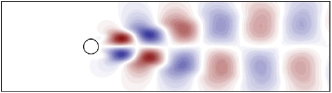
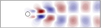
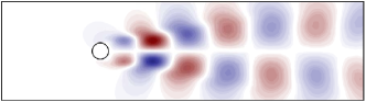
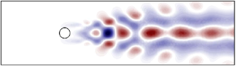
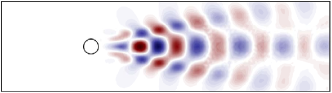
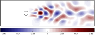
Figure 29: Left singular vectors of StreamVel via [HMT11]. (Sparse maps, approximation rank $r=5$, storage budget $T=48(m+n)$.) The columns of the matrix StreamVel describe the fluctuations of the streamwise velocity field about its mean value as a function of time. From top to bottom, the panels show the first nine computed left singular vectors of the matrix. The left-hand side is computed using [HMT11], while the right-hand side is computed from the exact flow field. The heatmap indicates the magnitude of the fluctuation. See Section 7.8.

This approach is not competitive with more modern techniques. Some of the deficiencies stem from truncating the singular vectors to rank $r$ at the first step of the procedure; see Figs. 29 and 30.

D.1.2 The [TYUC17] Method

In our previous paper, we developed and analyzed a sketching algorithm [69, Alg. 7] for low-rank matrix approximation. Our work contains a detailed theoretical analysis, prescriptions for choosing algorithm parameters, and an extensive numerical evaluation. We later discovered that this method is algebraically (but not numerically) equivalent to a proposal of Clarkson & Woodruff [20, Thm. 4.9]. The paper [20] also lacks reliable instructions for implementation.

This approach uses two dimension reduction maps that are indexed by two parameters $k,\ell$:

$$\bm{\Upsilon}\in\mathbb{F}^{\ell\times m}\quad\text{and}\quad\bm{\Omega}\in\mathbb{F}^{k\times n}\quad\text{where $k\leq\ell$.}$$

The sketch takes the form

$$\bm{X}=\bm{\Upsilon A}\quad\text{and}\quad\bm{Y}=\bm{A\Omega}^{*}.$$

To obtain a rank-$r$ approximation from the sketch, we compute a thin orthogonal–triangular decomposition:

$$\bm{Y}=:\bm{QR}\quad\text{where $\bm{Q}\in\mathbb{F}^{m\times k}$.}$$

Then we form the approximation:

(37) $$\hat{\bm{A}}_{\mathrm{tyuc}}:=\bm{Q}\llbracket{(\bm{\Upsilon}\bm{Q})^{\dagger}\bm{X}}\rrbracket_{r}.$$

Of course, we solve the least-squares problems, rather than computing and applying the pseudoinverse. We use a dense SVD or a randomized SVD [35] to calculate the best rank-$r$ approximation.

This method works well, but it uses more storage than necessary because $\ell$ needs to be somewhat larger than $k$. The algorithm can also be sensitive to the relative size of the parameters $k,\ell$.

D.1.3 The [Upa16] Method

In a paper on privacy-preserving matrix approximation, Upadhyay [71, Sec. 3] developed an algorithm that also serves for streaming low-rank matrix approximation. This method simplifies a far more complicated approach due to Boutsidis et al. [15, Sec. 6].

Upadhyay proposed the sketch Eqs. 4, 5, and 6, which depends on two parameters $k,s$. We are building on his idea in this paper. In contrast to our work, Upadhyay designs a rank-$r$ reconstruction algorithm using the “sketch-and-solve” framework; see Section 2.8.

His approach leads to the following algorithm. First, compute orthonormal bases $\bm{Q}$ and $\bm{P}$ for the range and co-range:

$$\bm{X}^{*} =:\bm{PR}_{1}\quad\text{where}\quad\bm{P}\in\mathbb{F}^{n\times k};$$

$$\bm{Y} =:\bm{QR}_{2}\quad\text{where}\quad\bm{Q}\in\mathbb{F}^{m\times k}.$$

Next, form thin singular value decompositions:

$$\bm{\Phi Q}=\bm{U}_{1}\bm{\Sigma}_{1}\bm{V}_{1}^{*}\in\mathbb{F}^{s\times k}\quad\text{and}\quad\bm{\Psi P}=\bm{U}_{2}\bm{\Sigma}_{2}\bm{V}_{2}^{*}\in\mathbb{F}^{s\times k}.$$

Construct the rank-$r$ approximation using the formula

(38) $$\hat{\bm{A}}_{\mathrm{upa}}:=\bm{Q}\bm{V}_{1}\bm{\Sigma}_{1}^{\dagger}\,\llbracket{\bm{U}_{1}^{*}\bm{Z}\bm{U}_{2}}\rrbracket_{r}\,\bm{\Sigma}_{2}^{\dagger}\bm{V}_{2}^{*}\bm{P}^{*}.$$

We use a truncated SVD to perform the rank truncation of the central matrix. Of course, we should take care in applying the pseudoinverses.

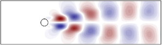
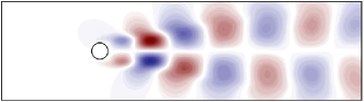
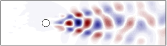
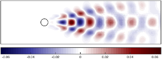
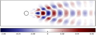
Figure 31: Left singular vectors of StreamVel via [Upa16]. (Sparse maps, approximation rank $r=5$, storage budget $T=48(m+n)$.) The columns of the matrix StreamVel describe the fluctuations of the streamwise velocity field about its mean value as a function of time. From top to bottom, the panels show the first nine computed left singular vectors of the matrix. The left-hand side is computed using [Upa16], while the right-hand side is computed from the exact flow field. The heatmap indicates the magnitude of the fluctuation. See Section 7.8.

Superficially, the approximation $\hat{\bm{A}}_{\mathrm{upa}}$ may appear similar to the approximation we developed in Eq. 12. Nevertheless, they are designed using different principles, and their performance is quite different in practice. The [Upa16] method cannot achieve high relative accuracy, even for matrices with rapid spectral decay. Furthermore, it has the bizarre feature that decreasing the rank parameter $r$ can actually make the approximation less reliable! See Figs. 31 and 32.

D.2 Spectra of Input Matrices

Figure 9 plots the spectrum of each of the synthetic and application matrices that we use in our experiments.

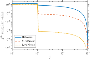
(a) Low-Rank + Noise

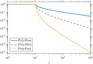
(b) Polynomial Decay

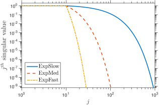
(c) Exponential Decay

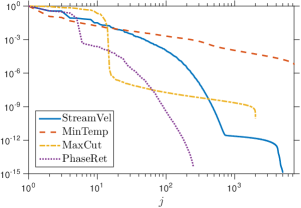
(d) Data Matrices

Figure 9: Spectra of input matrices. Plots of the singular value spectrum for an input matrix from each of the synthetic classes (LowRank, PolyDecay, ExpDecay with effective rank $R=10$) and from each of the real data classes (MinTemp, StreamVel, MaxCut, PhaseRetrieval) described in Section 7.3.

D.3 Insensitivity to the Dimension Reduction Map

Our first experiment is designed to show that the proposed rank-$r$ reconstruction formula Eq. 12 is insensitive to the distribution of the dimension reduction map at the oracle parameter values (Section 7.2.2) for synthetic input matrices.

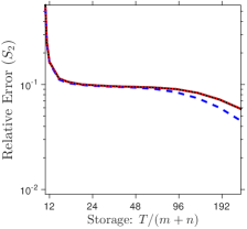
(a) LowRankHiNoise

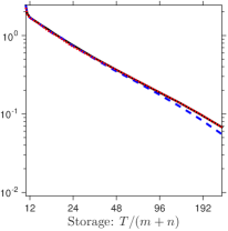
(b) LowRankMedNoise

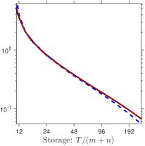
(c) LowRankLowNoise

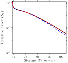
(d) PolyDecaySlow

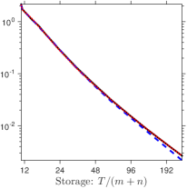
(e) PolyDecayMed

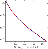
(f) PolyDecayFast

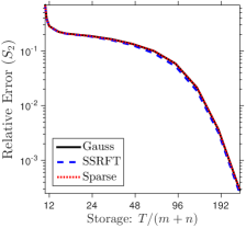
(g) ExpDecaySlow

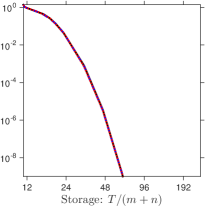
(h) ExpDecayMed

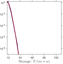
(i) ExpDecayFast

Figure 12: Insensitivity of proposed method to the dimension reduction map. (Effective rank $R=10$, approximation rank $r=10$, Schatten 2-norm.) We compare the oracle performance of the proposed fixed-rank approximation Eq. 12 implemented with Gaussian, SSRFT, or sparse dimension reduction maps. See Section D.3 for details.

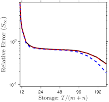
(a) LowRankHiNoise

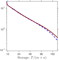
(b) LowRankMedNoise

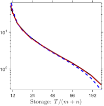
(c) LowRankLowNoise

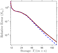
(d) PolyDecaySlow

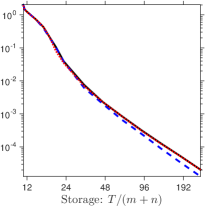
(e) PolyDecayMed

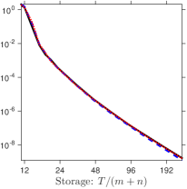
(f) PolyDecayFast

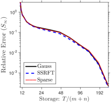
(g) ExpDecaySlow

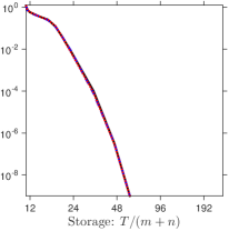
(h) ExpDecayMed

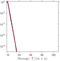
(i) ExpDecayFast

Figure 13: Insensitivity of proposed method to the dimension reduction map. (Effective rank $R=10$, approximation rank $r=10$, Schatten $\infty$-norm.) We compare the oracle performance of the proposed fixed-rank approximation Eq. 12 implemented with Gaussian, SSRFT, or sparse dimension reduction maps. See Section D.3 for details.

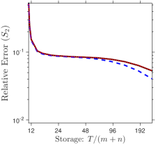
(a) LowRankHiNoise

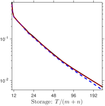
(b) LowRankMedNoise

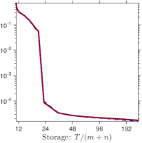
(c) LowRankLowNoise

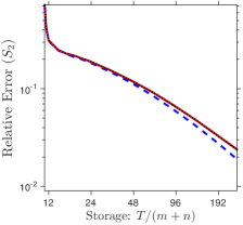
(d) PolyDecaySlow

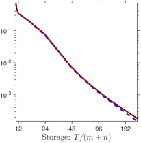
(e) PolyDecayMed

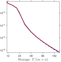
(f) PolyDecayFast

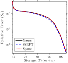
(g) ExpDecaySlow

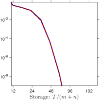
(h) ExpDecayMed

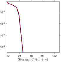
(i) ExpDecayFast

Figure 14: Insensitivity of proposed method to the dimension reduction map. (Effective rank $R=20$, approximation rank $r=10$, Schatten 2-norm.) We compare the oracle performance of the proposed fixed-rank approximation Eq. 12 implemented with Gaussian, SSRFT, or sparse dimension reduction maps. See Section D.3 for details.

We plot the oracle error for Eq. 12 as a function of storage budget $T$ for Gaussian, SSRFT, and sparse dimension reduction maps. See Figs. 10, 11, 12, 13, 14, and 15. The curves are almost identical, except that the unitary SSRFT map performs slightly better than the others when the storage budget is very large. Similar results hold for matrices drawn from real applications.

We have also found that the other reconstruction methods [HMT11], [TYUC17], and [Upa16] are insensitive to the choice of dimension reduction map. These observations justify the transfer of theoretical and empirical results for Gaussians to SSRFT and sparse dimension reduction maps.

D.4 Achieving the Oracle Performance

Next, we show that we can almost achieve the oracle error by implementing Eq. 12 with sketch size parameters chosen using our theory.

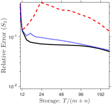
(a) LowRankHiNoise

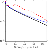
(b) LowRankMedNoise

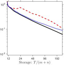
(c) LowRankLowNoise

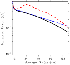
(d) PolyDecaySlow

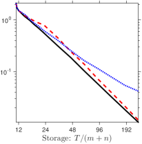
(e) PolyDecayMed

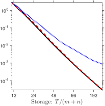
(f) PolyDecayFast

(g) ExpDecaySlow

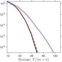
(h) ExpDecayMed

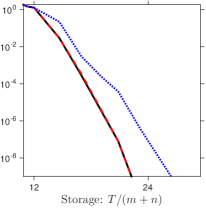
(i) ExpDecayFast

Figure 16: Relative error for proposed method with a priori parameters. (Gaussian maps, effective rank $R=5$, approximation rank $r=10$, Schatten $2$-norm.) We compare the oracle performance of the proposed fixed-rank approximation Eq. 12 with its performance at theoretically justified parameter values. See Section D.4 for details.

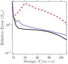
(a) LowRankHiNoise

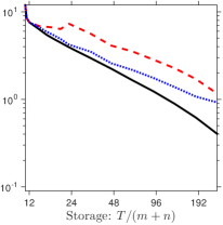
(b) LowRankMedNoise

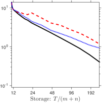
(c) LowRankLowNoise

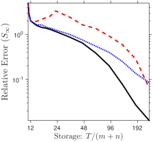
(d) PolyDecaySlow

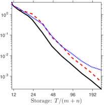
(e) PolyDecayMed

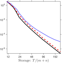
(f) PolyDecayFast

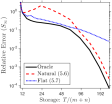
(g) ExpDecaySlow

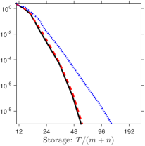
(h) ExpDecayMed

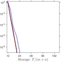
(i) ExpDecayFast

Figure 17: Relative error for proposed method with a priori parameters. (Gaussian maps, effective rank $R=5$, approximation rank $r=10$, Schatten $\infty$-norm.) We compare the oracle performance of the proposed fixed-rank approximation Eq. 12 with its performance at theoretically justified parameter values. See Section D.4 for details.

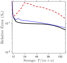
(a) LowRankHiNoise

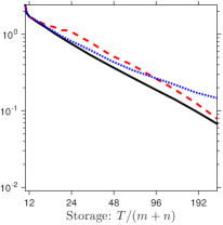
(b) LowRankMedNoise

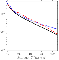
(c) LowRankLowNoise

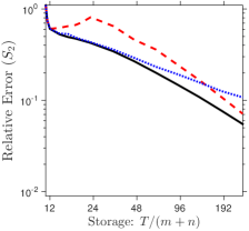
(d) PolyDecaySlow

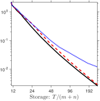
(e) PolyDecayMed

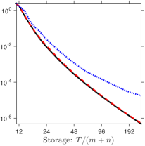
(f) PolyDecayFast

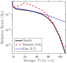
(g) ExpDecaySlow

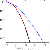
(h) ExpDecayMed

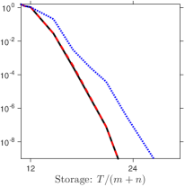
(i) ExpDecayFast

Figure 18: Relative error for proposed method with a priori parameters. (Gaussian maps, effective rank $R=10$, approximation rank $r=10$, Schatten $2$-norm.) We compare the oracle performance of the proposed fixed-rank approximation Eq. 12 with its performance at theoretically justified parameter values. See Section D.4 for details.

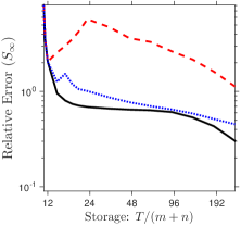
(a) LowRankHiNoise

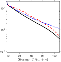
(b) LowRankMedNoise

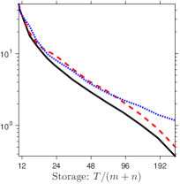
(c) LowRankLowNoise

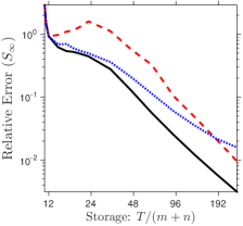
(d) PolyDecaySlow

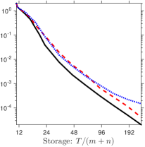
(e) PolyDecayMed

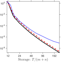
(f) PolyDecayFast

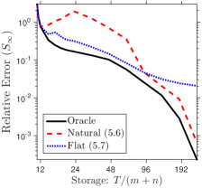
(g) ExpDecaySlow

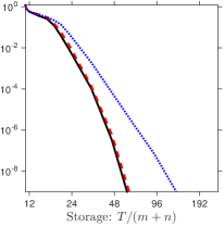
(h) ExpDecayMed

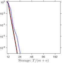
(i) ExpDecayFast

Figure 19: Relative error for proposed method with a priori parameters. (Gaussian maps, effective rank $R=10$, approximation rank $r=10$, Schatten $\infty$-norm.) We compare the oracle performance of the proposed fixed-rank approximation Eq. 12 with its performance at theoretically justified parameter values. See Section D.4 for details.

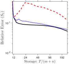
(a) LowRankHiNoise

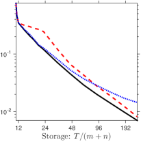
(b) LowRankMedNoise

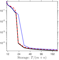
(c) LowRankLowNoise

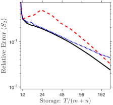
(d) PolyDecaySlow

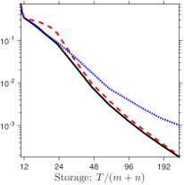
(e) PolyDecayMed

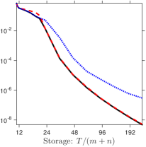
(f) PolyDecayFast

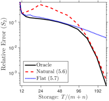
(g) ExpDecaySlow

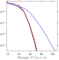
(h) ExpDecayMed

(i) ExpDecayFast

Figure 20: Relative error for proposed method with a priori parameters. (Gaussian maps, effective rank $R=20$, approximation rank $r=10$, Schatten $2$-norm.) We compare the oracle performance of the proposed fixed-rank approximation Eq. 12 with its performance at theoretically justified parameter values. See Section D.4 for details.

We perform the following experiment. For synthetic input matrices, we compare the oracle performance (Section 7.2.2) of our rank-$r$ approximation Eq. 12 with its performance at the theoretical parameters proposed in Section 5.4. (In the formula Eq. 21 for a flat spectrum, we set the tail location $\hat{\varrho}=r$.) We use Gaussian dimension reduction maps, but equivalent results hold for other types of dimension reduction maps. Plots of the results appear in Figs. 16, 17, 18, 19, 20, and 21.

For most of the examples, the general parameter choice Eq. 20 is able to deliver a relative error that tracks the oracle error closely. The parameter choice Eq. 21 for a flat spectrum works somewhat better for matrices whose spectral tail exhibits slow decay (LowRankLowNoise, LowRankMedNoise, LowRankHiNoise). We also learn that the theoretical formulas are not entirely reliable when the storage budget is very small. Matrices with a lot of tail energy (LowRankHiNoise, PolyDecaySlow) are very hard to approximate accurately with a sketching algorithm, so it is not surprising that our theoretical parameter choices fall short of the oracle parameters in these cases.

D.5 Algorithm Comparisons for Synthetic Instances

We compared all four of the reconstruction formulas at the oracle parameters for a wide range of synthetic problem instances. See Section 7.6 for details.

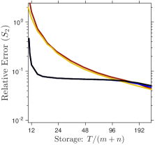
(a) LowRankHiNoise

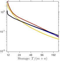
(b) LowRankMedNoise

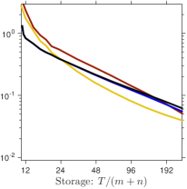
(c) LowRankLowNoise

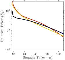
(d) PolyDecaySlow

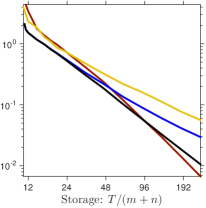
(e) PolyDecayMed

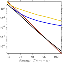
(f) PolyDecayFast

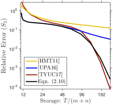
(g) ExpDecaySlow

(h) ExpDecayMed

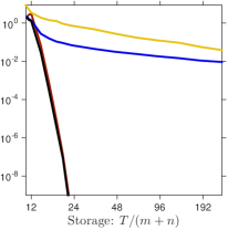
(i) ExpDecayFast

Figure 22: Comparison of reconstruction formulas: Synthetic examples. (Gaussian maps, effective rank $R=5$, approximation rank $r=10$, Schatten 2-norm.) We compare the oracle error achieved by the proposed fixed-rank approximation Eq. 12 against methods Eqs. 38 and 37 from the literature. See Section 7.2.2 for details.

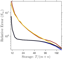
(a) LowRankHiNoise

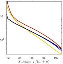
(b) LowRankMedNoise

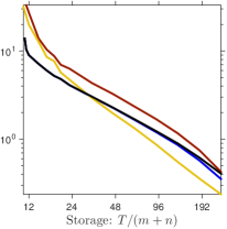
(c) LowRankLowNoise

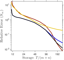
(d) PolyDecaySlow

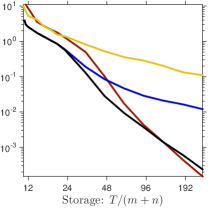
(e) PolyDecayMed

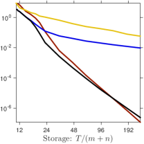
(f) PolyDecayFast

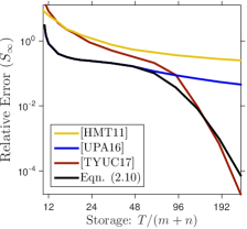
(g) ExpDecaySlow

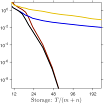
(h) ExpDecayMed

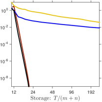
(i) ExpDecayFast

Figure 23: Comparison of reconstruction formulas: Synthetic examples. (Gaussian maps, effective rank $R=5$, approximation rank $r=10$, Schatten $\infty$-norm.) We compare the oracle error achieved by the proposed fixed-rank approximation Eq. 12 against methods Eqs. 38 and 37 from the literature. See Section 7.2.2 for details.

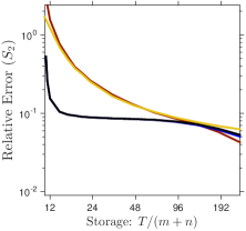
(a) LowRankHiNoise

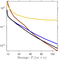
(b) LowRankMedNoise

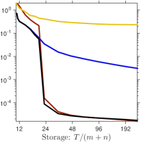
(c) LowRankLowNoise

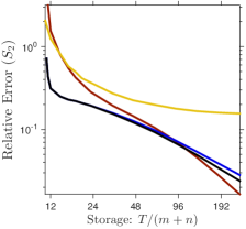
(d) PolyDecaySlow

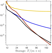
(e) PolyDecayMed

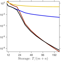
(f) PolyDecayFast

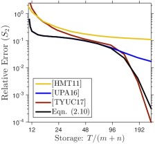
(g) ExpDecaySlow

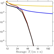
(h) ExpDecayMed

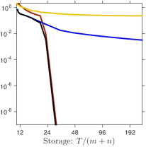
(i) ExpDecayFast

Figure 25: Comparison of reconstruction formulas: Synthetic examples. (Gaussian maps, effective rank $R=20$, approximation rank $r=10$, Schatten 2-norm.) We compare the oracle error achieved by the proposed fixed-rank approximation Eq. 12 against methods Eqs. 38 and 37 from the literature. See Section 7.2.2 for details.

Figures 22, 23, 25, and 26 contain the results for matrices with effective rank $R=5$ and $R=20$ with relative error measured in Schatten $2$-norm and Schatten $\infty$-norm.

D.6 Algorithm Comparisons for Real Data Instances

In this experiment, we compared all four of the reconstruction formulas at the oracle parameters and at theoretically chosen parameters for several application examples.

Here are the details of the a priori parameter selections for the several methods. For the proposed method Eq. 12, we use the “natural” parameter choice Eq. 20 that follows from our theoretical analysis. The [Upa16] algorithm uses the same sketch—but lacks a comparable theory—so we instantiate it with the parameters Eq. 20. For [TYUC17], we assume that the input matrix $\bm{A}\in\mathbb{F}^{m\times n}$ is tall ($m\geq n$), and we use the theoretically motivated parameter values

$$k=\max\{r+\alpha+1,\lfloor(T-n\alpha)/(m+2n)\rfloor\}\quad\text{and}\quad\ell=\lfloor(T-km)/n\rfloor.$$

This choice adapts the arguments in [69, Sec. 4.5.2] to use the current definition of the storage budget $T$. The [HMT11] algorithm does not have any free parameters.

D.7 Flow-Field Reconstruction

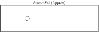
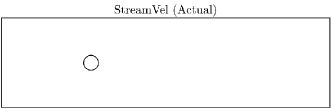
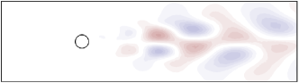
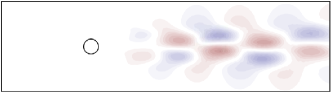
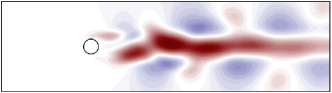
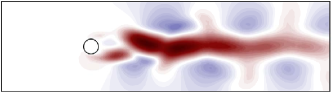
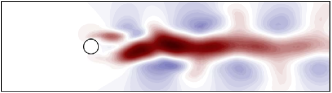
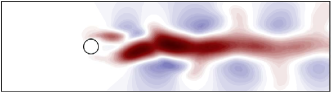
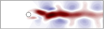
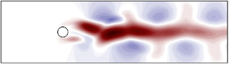
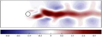
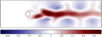
Figure 28: Approximation of StreamVel via Eq. 12. (Sparse maps, approximation rank $r=10$, storage budget $T=48(m+n)$.) The columns of the matrix StreamVel describe the fluctuations of the streamwise velocity field about its mean value as a function of time. From top to bottom, the panels show columns $1,1001,1501,2001,2501,3001,3501,4001$. The left-hand side displays the approximation Eq. 12 of the flow field, and the right-hand side displays the exact flow field. The heatmap indicates the magnitude of the fluctuation. See Section 7.8.

Fig. 28 illustrates the streamwise velocity field StreamVel and its rank-$10$ approximation via Eq. 12 using storage budget $T=48(m+n)$ and the parameter choices Eq. 20. We see that the approximation captures the large-scale features of the flow, although there are small errors visible for the higher-order singular vectors.

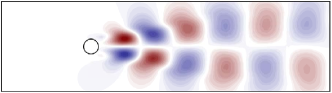
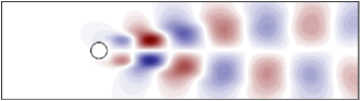
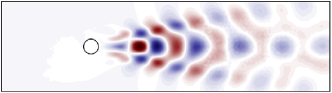
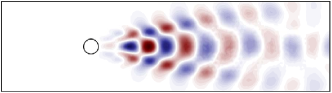
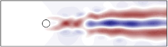
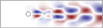
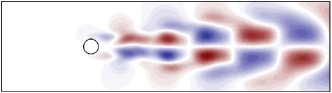
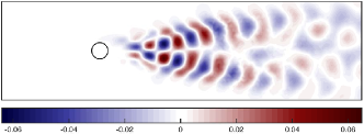
Figure 30: Left singular vectors of StreamVel via [HMT11]. (Sparse maps, approximation rank $r=10$, storage budget $T=48(m+n)$.) The columns of the matrix StreamVel describe the fluctuations of the streamwise velocity field about its mean value as a function of time. From top to bottom, the panels show the first nine computed left singular vectors of the matrix. The left-hand side is computed using [HMT11], while the right-hand side is computed from the exact flow field. The heatmap indicates the magnitude of the fluctuation. See Section 7.8.

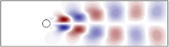
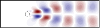
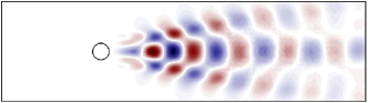
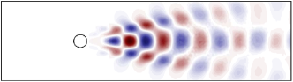
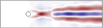
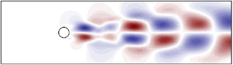
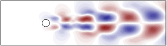
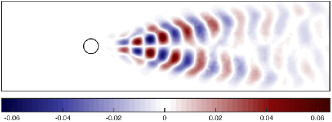
Figure 32: Left singular vectors of StreamVel via [Upa16]. (Sparse maps, approximation rank $r=10$, storage budget $T=48(m+n)$.) The columns of the matrix StreamVel describe the fluctuations of the streamwise velocity field about its mean value as a function of time. From top to bottom, the panels show the first nine computed left singular vectors of the matrix. The left-hand side is computed using [Upa16], while the right-hand side is computed from the exact flow field. The heatmap indicates the magnitude of the fluctuation. See Section 7.8.

We also performed the same experiment with the algorithms [HMT11], [Upa16], and [TYUC17]. We set the truncation rank $r=5$ and $r=10$ to see whether this change affects the behavior of the methods. We plot the leading left singular vectors of the flow fields in Figs. 29, 30, 31, 32, and 33. For truncation $r=10$, all of the algorithms produce reasonable results. Nevertheless, with algorithms [HMT11], [Upa16], and [TYUC17], the singular vector estimates for rank $6,7,8,9$ start to deviate from the singular vectors of the original matrix.

When we change the truncation rank to $r=5$, our methods [TYUC17] and Eq. 12 give exactly the same singular vector estimates as with $r=10$, by construction of the algorithm. On the other hand, the methods [HMT11] and [Upa16] behave far worse when $r=5$ than when $r=10$. This feature is both strange and dissatisfying. By itself, this lack of stability is already enough to disqualify the algorithms [HMT11] and [Upa16] from practical use.

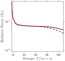
(a) LowRankHiNoise

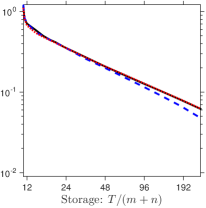
(b) LowRankMedNoise

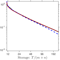
(c) LowRankLowNoise

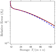
(d) PolyDecaySlow

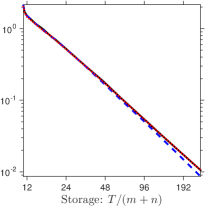
(e) PolyDecayMed

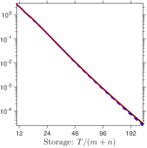
(f) PolyDecayFast

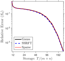
(g) ExpDecaySlow

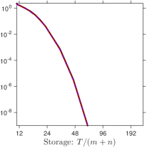
(h) ExpDecayMed

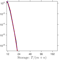
(i) ExpDecayFast

Figure 10: Insensitivity of proposed method to the dimension reduction map. (Effective rank $R=5$, approximation rank $r=10$, Schatten 2-norm.) We compare the oracle performance of the proposed fixed-rank approximation Eq. 12 implemented with Gaussian, SSRFT, or sparse dimension reduction maps. See Section D.3 for details.

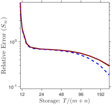
(a) LowRankHiNoise

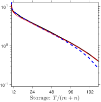
(b) LowRankMedNoise

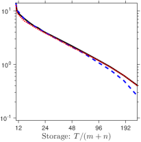
(c) LowRankLowNoise

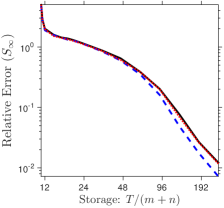
(d) PolyDecaySlow

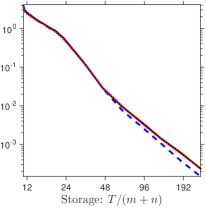
(e) PolyDecayMed

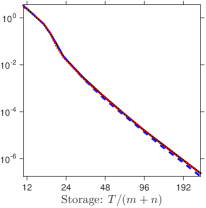
(f) PolyDecayFast

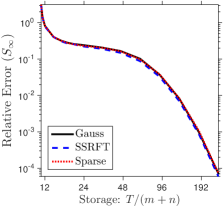
(g) ExpDecaySlow

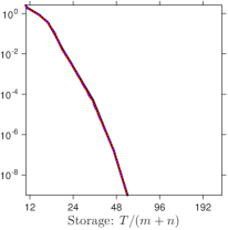
(h) ExpDecayMed

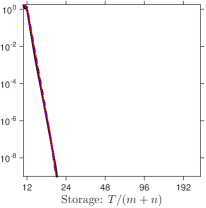
(i) ExpDecayFast

Figure 11: Insensitivity of proposed method to the dimension reduction map. (Effective rank $R=5$, approximation rank $r=10$, Schatten $\infty$-norm.) We compare the oracle performance of the proposed fixed-rank approximation Eq. 12 implemented with Gaussian, SSRFT, or sparse dimension reduction maps. See Section D.3 for details.

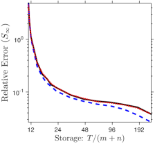
(a) LowRankHiNoise

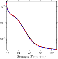
(b) LowRankMedNoise

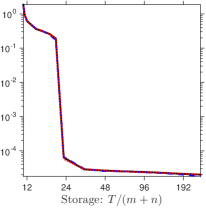
(c) LowRankLowNoise

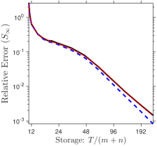
(d) PolyDecaySlow

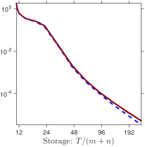
(e) PolyDecayMed

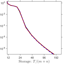
(f) PolyDecayFast

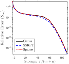
(g) ExpDecaySlow

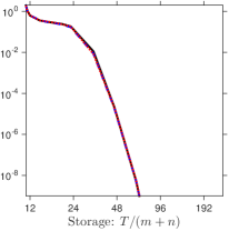
(h) ExpDecayMed

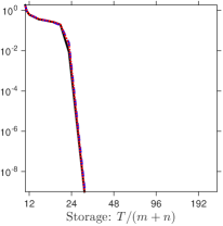
(i) ExpDecayFast

Figure 15: Insensitivity of proposed method to the dimension reduction map. (Effective rank $R=20$, approximation rank $r=10$, Schatten $\infty$-norm.) We compare the oracle performance of the proposed fixed-rank approximation Eq. 12 implemented with Gaussian, SSRFT, or sparse dimension reduction maps. See Section D.3 for details.

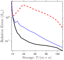
(a) LowRankHiNoise

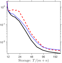
(b) LowRankMedNoise

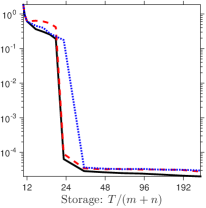
(c) LowRankLowNoise

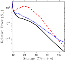
(d) PolyDecaySlow

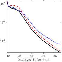
(e) PolyDecayMed

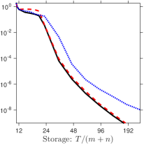
(f) PolyDecayFast

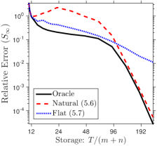
(g) ExpDecaySlow

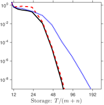
(h) ExpDecayMed

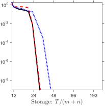
(i) ExpDecayFast

Figure 21: Relative error for proposed method with a priori parameters. (Gaussian maps, effective rank $R=20$, approximation rank $r=10$, Schatten $\infty$-norm.) We compare the oracle performance of the proposed fixed-rank approximation Eq. 12 with its performance at theoretically justified parameter values. See Section D.4 for details.

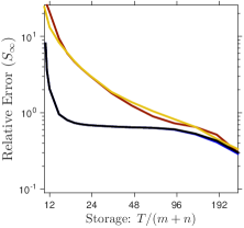
(a) LowRankHiNoise

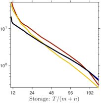
(b) LowRankMedNoise

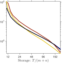
(c) LowRankLowNoise

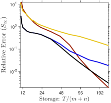
(d) PolyDecaySlow

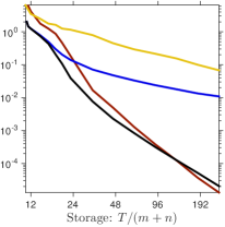
(e) PolyDecayMed

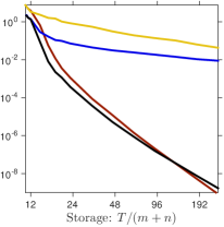
(f) PolyDecayFast

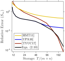
(g) ExpDecaySlow

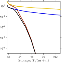
(h) ExpDecayMed

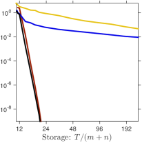
(i) ExpDecayFast

Figure 24: Comparison of reconstruction formulas: Synthetic examples. (Gaussian maps, effective rank $R=10$, approximation rank $r=10$, Schatten $\infty$-norm.) We compare the oracle error achieved by the proposed fixed-rank approximation Eq. 12 against methods Eqs. 38 and 37 from the literature. See Section 7.2.2 for details.

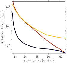
(a) LowRankHiNoise

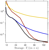
(b) LowRankMedNoise

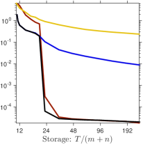
(c) LowRankLowNoise

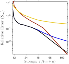
(d) PolyDecaySlow

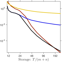
(e) PolyDecayMed

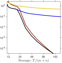
(f) PolyDecayFast

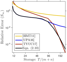
(g) ExpDecaySlow

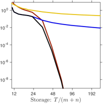
(h) ExpDecayMed

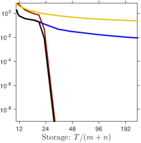
(i) ExpDecayFast

Figure 26: Comparison of reconstruction formulas: Synthetic examples. (Gaussian maps, effective rank $R=20$, approximation rank $r=10$, Schatten $\infty$-norm.) We compare the oracle error achieved by the proposed fixed-rank approximation Eq. 12 against methods Eqs. 38 and 37 from the literature. See Section 7.2.2 for details.

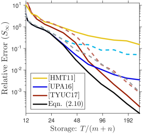
(a) MinTemp ($r=10$)

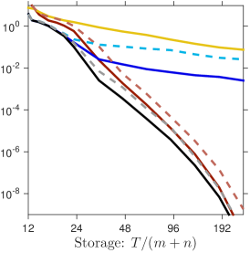
(b) StreamVel ($r=10$)

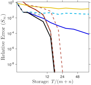
(c) MaxCut ($r=1$)

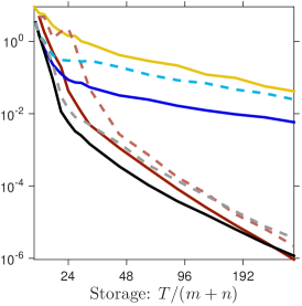
(d) MaxCut ($r=14$)

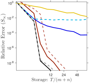
(e) PhaseRetrieval ($r=1$)

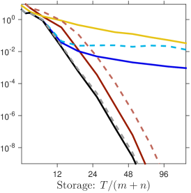
(f) PhaseRetrieval ($r=5$)

Figure 27: Comparison of reconstruction formulas: Real data examples. (Sparse maps, Schatten $\infty$-norm.) We compare the relative error achieved by the proposed fixed-rank approximation Eq. 12 against methods Eqs. 38 and 37 from the literature. Solid lines are oracle errors; dashed lines are errors with “natural” parameter choices. See Section 7.7 for details.

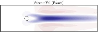
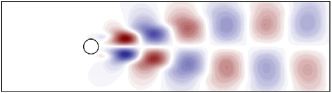
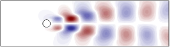
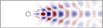
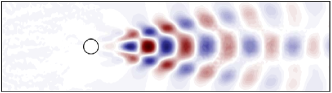
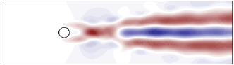
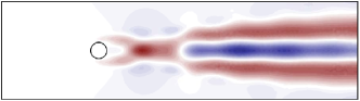
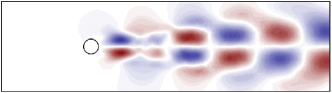
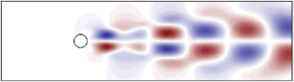
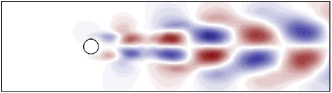
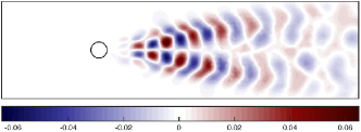
Figure 33: Left singular vectors of StreamVel via [TYUC17]. (Sparse maps, approximation rank $r=10$, storage budget $T=48(m+n)$.) The columns of the matrix StreamVel describe the fluctuations of the streamwise velocity field about its mean value as a function of time. From top to bottom, the panels show the first nine computed left singular vectors of the matrix. The left-hand side is computed using [TYUC17], while the right-hand side is computed from the exact flow field. The heatmap indicates the magnitude of the fluctuation. See Section 7.8.

References

- [1] Physical sciences division, national oceanic and atmospheric administration, Feb. 2019, https://www.esrl.noaa.gov/psd/.
- [2] D. Achlioptas, Database-friendly random projections: Johnson–Lindenstrauss with binary coins, J. Comput. System Sci., 66 (2003), pp. 671–687.
- [3] N. Ailon and B. Chazelle, The fast Johnson-Lindenstrauss transform and approximate nearest neighbors, SIAM J. Comput., 39 (2009), pp. 302–322, https://doi.org/10.1137/060673096, http://dx.doi.org/10.1137/060673096.
- [4] N. Alon, P. B. Gibbons, Y. Matias, and M. Szegedy, Tracking join and self-join sizes in limited storage, J. Comput. System Sci., 64 (2002), pp. 719–747, https://doi.org/10.1006/jcss.2001.1813, https://doi.org/10.1006/jcss.2001.1813. Special issue on PODS 1999 (Philadelphia, PA).
- [5] N. Alon, Y. Matias, and M. Szegedy, The space complexity of approximating the frequency moments, in Proceedings of the Twenty-eighth Annual ACM Symposium on the Theory of Computing (Philadelphia, PA, 1996), ACM, New York, 1996, pp. 20–29, https://doi.org/10.1145/237814.237823, https://doi.org/10.1145/237814.237823.
- [6] W. Austin, G. Ballard, and T. G. Kolda, Parallel tensor compression for large-scale scientific data, in 2016 IEEE Intl. Symp. Parallel and Distributed Processing, 2016, pp. 912–922.
- [7] H. Avron and S. Toledo, Randomized algorithms for estimating the trace of an implicit symmetric positive semi-definite matrix, J. ACM, 58 (2011), pp. Art. 8, 17, https://doi.org/10.1145/1944345.1944349, https://doi.org/10.1145/1944345.1944349.
- [8] A. H. Baker, H. Xu, J. M. Dennis, M. N. Levy, D. Nychka, S. A. Mickelson, J. Edwards, M. Vertenstein, and A. Wegener, A methodology for evaluating the impact of data compression on climate simulation data, in Proc. 23rd ACM Intl. Symp. High-Performance Parallel and Distributed Computing, 2014, pp. 203–214.
- [9] R. Baurle, Modeling of high speed reacting flows: Established practices and future challenges, in 42nd AIAA Aerospace Sciences Meeting and Exhibit, 2004, p. 267.
- [10] A. Bejan, Convection heat transfer, John Wiley & Sons, 2013.
- [11] R. Bhatia, Matrix analysis, vol. 169 of Graduate Texts in Mathematics, Springer-Verlag, New York, 1997, https://doi.org/10.1007/978-1-4612-0653-8, https://doi.org/10.1007/978-1-4612-0653-8.
- [12] J. Bourgain, S. Dirksen, and J. Nelson, Toward a unified theory of sparse dimensionality reduction in Euclidean space, Geom. Funct. Anal., 25 (2015), pp. 1009–1088, https://doi.org/10.1007/s00039-015-0332-9, http://dx.doi.org/10.1007/s00039-015-0332-9.
- [13] C. Boutsidis and A. Gittens, Improved matrix algorithms via the subsampled randomized Hadamard transform, SIAM J. Matrix Anal. Appl., 34 (2013), pp. 1301–1340, https://doi.org/10.1137/120874540, http://dx.doi.org/10.1137/120874540.
- [14] C. Boutsidis, D. Woodruff, and P. Zhong, Optimal principal component analysis in distributed and streaming models. Available at http://arXiv.org/abs/1504.06729, July 2016.
- [15] C. Boutsidis, D. Woodruff, and P. Zhong, Optimal principal component analysis in distributed and streaming models, in Proc. 48th ACM Symp. Theory of Computing (STOC 2016), Cambridge, MA, 2016.
- [16] M. Brand, Fast low-rank modifications of the thin singular value decomposition, Linear Algebra and its Applications, 415 (2006), pp. 20 – 30, https://doi.org/https://doi.org/10.1016/j.laa.2005.07.021, http://www.sciencedirect.com/science/article/pii/S0024379505003812. Special Issue on Large Scale Linear and Nonlinear Eigenvalue Problems.
- [17] J. Calhoun, F. Cappello, L. N. Olson, M. Snir, and W. D. Gropp, Exploring the feasibility of lossy compression for PDE simulations, The International Journal of High Performance Computing Applications, (2018), p. 1094342018762036, https://doi.org/10.1177/1094342018762036.
- [18] S. Castruccio and M. G. Genton, Compressing an ensemble with statistical models: An algorithm for global 3D spatio-temporal temperature, Technometrics, 58 (2016), pp. 319–328.
- [19] CERN, Processing: What to record, Feb. 2019, https://home.cern/science/computing/processing-what-record.
- [20] K. L. Clarkson and D. P. Woodruff, Numerical linear algebra in the streaming model, in Proc. 41st ACM Symp. Theory of Computing (STOC), Bethesda, 2009.
- [21] K. L. Clarkson and D. P. Woodruff, Low rank approximation and regression in input sparsity time, in Proc. 45th ACM Symp. Theory of Computing (STOC), ACM, New York, 2013, pp. 81–90, https://doi.org/10.1145/2488608.2488620, http://dx.doi.org/10.1145/2488608.2488620.
- [22] M. Cohen, Nearly tight oblivious subspace embeddings by trace inequalities, in Proc. 27th ACM-SIAM Symp. Discrete Algorithms (SODA), Arlington, Jan. 2016, pp. 278–287.
- [23] M. B. Cohen, S. Elder, C. Musco, C. Musco, and M. Persu, Dimensionality reduction for k-means clustering and low rank approximation, in Proc. 47th ACM Symp. Theory of Computing (STOC), ACM, 2015, pp. 163–172.
- [24] J. D. Dixon, Estimating extremal eigenvalues and condition numbers of matrices, SIAM J. Numer. Anal., 20 (1983), pp. 812–814, https://doi.org/10.1137/0720053, https://doi.org/10.1137/0720053.
- [25] J. B. Drake, Climate modeling for scientists and engineers, SIAM, 2014.
- [26] D. Feldman, M. Volkov, and D. Rus, Dimensionality reduction of massive sparse datasets using coresets, in Adv. Neural Information Processing Systems 29 (NIPS), 2016.
- [27] A. Frieze, R. Kannan, and S. Vempala, Fast Monte-Carlo algorithms for finding low-rank approximations, J. Assoc. Comput. Mach., 51 (2004), pp. 1025–1041, https://doi.org/10.1145/1039488.1039494, http://dx.doi.org/10.1145/1039488.1039494.
- [28] E. Garnier, N. Adams, and P. Sagaut, Large eddy simulation for compressible flows, Springer Science & Business Media, 2009.
- [29] M. Ghashami, E. Liberty, J. M. Phillips, and D. P. Woodruff, Frequent directions: simple and deterministic matrix sketching, SIAM J. Comput., 45 (2016), pp. 1762–1792, https://doi.org/10.1137/15M1009718, https://doi-org.clsproxy.library.caltech.edu/10.1137/15M1009718.
- [30] M. X. Goemans and D. Williamson, Improved approximation algorithms for maximum cut and satisfiability problems using semidefinite programming, J. Assoc. Comput. Mach., 42 (1995), pp. 1115–1145.
- [31] S. Gratton and D. Titley-Peloquin, Improved bounds for small-sample estimation, SIAM J. Matrix Anal. Appl., 39 (2018), pp. 922–931, https://doi.org/10.1137/17M1137541, https://doi.org/10.1137/17M1137541.
- [32] A. Griewank and A. Walther, Algorithm 799: Revolve: An implementation of checkpointing for the reverse or adjoint mode of computational differentiation, ACM Trans. Math. Softw., 26 (2000), pp. 19–45, https://doi.org/10.1145/347837.347846, http://doi.acm.org/10.1145/347837.347846.
- [33] J. Guinness and D. Hammerling, Compression and conditional emulation of climate model output, J. Amer. Stat. Assoc., (2017).
- [34] N. Halko, P.-G. Martinsson, Y. Shkolnisky, and M. Tygert, An algorithm for the principal component analysis of large data sets, SIAM J. Sci. Comput., 33 (2011), pp. 2580–2594, https://doi.org/10.1137/100804139, https://doi-org.clsproxy.library.caltech.edu/10.1137/100804139.
- [35] N. Halko, P. G. Martinsson, and J. A. Tropp, Finding structure with randomness: probabilistic algorithms for constructing approximate matrix decompositions, SIAM Rev., 53 (2011), pp. 217–288.
- [36] N. J. Higham, Matrix nearness problems and applications, in Applications of matrix theory (Bradford, 1988), Oxford Univ. Press, New York, 1989, pp. 1–27.
- [37] M. Hinze, A. Walther, and J. Sternberg, An optimal memory-reduced procedure for calculating adjoints of the instationary navier-stokes equations, Optimal Control Applications and Methods, 27 (2006), pp. 19–40, https://doi.org/10.1002/oca.771, https://onlinelibrary.wiley.com/doi/abs/10.1002/oca.771, https://arxiv.org/abs/https://onlinelibrary.wiley.com/doi/pdf/10.1002/oca.771.
- [38] R. Horstmeyer, R. Y. Chen, X. Ou, B. Ames, J. A. Tropp, and C. Yang, Solving ptychography with a convex relaxation, New J. Physics, 17 (2015), p. 053044.
- [39] M. F. Hutchinson, A stochastic estimator of the trace of the influence matrix for Laplacian smoothing splines, Comm. Statist. Simulation Comput., 18 (1989), pp. 1059–1076, https://doi.org/10.1080/03610918908812806, https://doi.org/10.1080/03610918908812806.
- [40] P. Indyk and R. Motwani, Approximate nearest neighbors: Towards removing the curse of dimensionality, in Proc. 30th ACM Symp. Theory of Computing (STOC), STOC ’98, New York, NY, USA, 1998, ACM, pp. 604–613, https://doi.org/10.1145/276698.276876, http://doi.acm.org/10.1145/276698.276876.
- [41] W. B. Johnson and J. Lindenstrauss, Extensions of Lipszhitz mapping into Hilbert space, Contemp. Math., 26 (1984), pp. 189–206.
- [42] I. T. Jolliffe, Principal component analysis, Springer Series in Statistics, Springer-Verlag, New York, second ed., 2002.
- [43] Y. Li, H. L. Nguyen, and D. P. Woodruff, Turnstile streaming algorithms might as well be linear sketches, in Proc. 46th ACM Symp. Theory of Computing (STOC), ACM, New York, 2014, pp. 174–183.
- [44] E. Liberty, Accelerated dense random projections, PhD thesis, Yale Univ., New Haven, 2009.
- [45] M. Lopes, S. Wang, and M. Mahoney, Error estimation for randomized least-squares algorithms via the bootstrap, in Proc. 32nd Ann. Conf. Neural Information Processing Systems, Vancouver, Dec. 2018.
- [46] M. W. Mahoney, Randomized algorithms for matrices and data, Found. Trends Mach. Learning, 3 (2011), pp. 123–224.
- [47] M. R. Malik, B. J. Isaac, A. Coussement, P. J. Smith, and A. Parente, Principal component analysis coupled with nonlinear regression for chemistry reduction, Combustion and Flame, 187 (2018), pp. 30–41.
- [48] P.-G. Martinsson, Randomized methods for matrix computations. Available at http://arXiv.org/abs/1607.01649v3, Feb. 2019.
- [49] P.-G. Martinsson, V. Rokhlin, and M. Tygert, A randomized algorithm for the decomposition of matrices, Appl. Comput. Harmon. Anal., 30 (2011), pp. 47–68, https://doi.org/10.1016/j.acha.2010.02.003, http://dx.doi.org/10.1016/j.acha.2010.02.003.
- [50] X. Meng and M. W. Mahoney, Low-distortion subspace embeddings in input-sparsity time and applications to robust linear regression, in Proc. 45th ACM Symp. Theory of Computing (STOC), ACM, New York, 2013, pp. 91–100, https://doi.org/10.1145/2488608.2488621, http://dx.doi.org/10.1145/2488608.2488621.
- [51] F. R. Menter, M. Kuntz, and R. Langtry, Ten years of industrial experience with the sst turbulence model, Turbulence, heat and mass transfer, 4 (2003), pp. 625–632.
- [52] R. Moarref, A. S. Sharma, J. A. Tropp, and B. J. McKeon, Model-based scaling and prediction of the streamwise energy intensity in high-Reynolds number turbulent channels, J. Fluid Mech., 734 (2013), pp. 275–316. Available at http://arXiv.org/abs/1302.1594.
- [53] S. Muthukrishnan, Data streams: algorithms and applications, Found. Trends Theor. Comput. Sci., 1 (2005), pp. 117–236.
- [54] J. Nelson and H. L. Nguyen, OSNAP: faster numerical linear algebra algorithms via sparser subspace embeddings, in 2013 IEEE 54th Symp. Foundations of Computer Science (FOCS), IEEE Computer Soc., Los Alamitos, CA, 2013, pp. 117–126, https://doi.org/10.1109/FOCS.2013.21, http://dx.doi.org/10.1109/FOCS.2013.21.
- [55] J. Nelson and H. L. Nguyen, Lower bounds for oblivious subspace embeddings, in Automata, languages, and programming. Part I, vol. 8572 of Lecture Notes in Comput. Sci., Springer, Heidelberg, 2014, pp. 883–894, https://doi.org/10.1007/978-3-662-43948-7_73, http://dx.doi.org/10.1007/978-3-662-43948-7_73.
- [56] C. H. Papadimitriou, P. Raghavan, H. Tamaki, and S. Vempala, Latent semantic indexing: a probabilistic analysis, J. Comput. System Sci., 61 (2000), pp. 217–235, https://doi.org/10.1006/jcss.2000.1711, http://dx.doi.org/10.1006/jcss.2000.1711. Special issue on the Seventeenth ACM SIGACT-SIGMOD-SIGART Symposium on Principles of Database Systems (Seattle, WA, 1998).
- [57] S. Patankar, Numerical heat transfer and fluid flow, CRC press, 1980.
- [58] R. W. Reynolds, N. A. Rayner, T. M. Smith, D. C. Stokes, and W. Wang, An improved in situ and satellite sst analysis for climate, J. Climate, 15 (2002), pp. 1609–1625.
- [59] R. W. Reynolds, T. M. Smith, C. Liu, D. B. Chelton, K. S. Casey, and M. G. Schlax, Daily high-resolution-blended analyses for sea surface temperature, J. Climate, 20 (2007), pp. 5473–5496.
- [60] V. Rokhlin, A. Szlam, and M. Tygert, A randomized algorithm for principal component analysis, SIAM J. Matrix Anal. Appl., 31 (2009), pp. 1100–1124, https://doi.org/10.1137/080736417, https://doi-org.clsproxy.library.caltech.edu/10.1137/080736417.
- [61] F. Roosta-Khorasani and U. Ascher, Improved bounds on sample size for implicit matrix trace estimators, Found. Comput. Math., 15 (2015), pp. 1187–1212, https://doi.org/10.1007/s10208-014-9220-1, https://doi.org/10.1007/s10208-014-9220-1.
- [62] P. Sagaut, Large eddy simulation for incompressible flows: an introduction, Springer Science & Business Media, 2006.
- [63] T. Sarlós, Improved approximation algorithms for large matrices via random projections, in Proc. 47th Ann. IEEE Symposium on Foundations of Computer Science (FOCS), Berkeley, 2006.
- [64] S. W. Son, Z. Chen, W. Hendrix, A. Agrawal, W.-k. Liao, and A. Choudhary, Data compression for the exascale computing era-survey, Supercomputing frontiers and innovations, 1 (2014), pp. 76–88.
- [65] Y. Sun, Y. Guo, J. A. Tropp, and M. Udell, Low-rank tucker approximation of a tensor from streaming data. Manuscript, Oct. 2018.
- [66] Y. Sun, Y. Guo, J. A. Tropp, and M. Udell, Tensor random projection for low memory dimension reduction, in NeurIPS Workshop on Relational Representation Learning, 2018, https://r2learning.github.io/assets/papers/CameraReadySubmission%2041.pdf
- [67] J. A. Tropp, Improved analysis of the subsampled randomized Hadamard transform, Adv. Adapt. Data Anal., 3 (2011), pp. 115–126, https://doi.org/10.1142/S1793536911000787, http://dx.doi.org/10.1142/S1793536911000787.
- [68] J. A. Tropp, A. Yurtsever, M. Udell, and V. Cevher, Fixed-rank approximation of a positive-semidefinite matrix from streaming data, in Adv. Neural Information Processing Systems 30 (NIPS), Long Beach, Dec. 2017.
- [69] J. A. Tropp, A. Yurtsever, M. Udell, and V. Cevher, Practical sketching algorithms for low-rank matrix approximation, SIAM J. Matrix Anal. Appl., 38 (2017), pp. 1454–1485.
- [70] J. A. Tropp, A. Yurtsever, M. Udell, and V. Cevher, Randomized single-view algorithms for low-rank matrix approximation, ACM Report 2017-01, Caltech, Pasadena, Jan. 2017. Available at http://arXiv.org/abs/1609.00048, v1.
- [71] J. Upadhyay, Fast and space-optimal low-rank factorization in the streaming model with application in differential privacy. Available at http://arXiv.org/abs/1604.01429, Apr. 2016.
- [72] J. Woodring, S. Mniszewski, C. Brislawn, D. DeMarle, and J. Ahrens, Revisiting wavelet compression for large-scale climate data using JPEG 2000 and ensuring data precision, in 2011 IEEE Symp. Large Data Analysis and Visualization (LDAV), 2011, pp. 31–38.
- [73] D. P. Woodruff, Sketching as a tool for numerical linear algebra, Found. Trends Theor. Comput. Sci., 10 (2014), pp. iv+157.
- [74] F. Woolfe, E. Liberty, V. Rokhlin, and M. Tygert, A fast randomized algorithm for the approximation of matrices, Appl. Comput. Harmon. Anal., 25 (2008), pp. 335–366.
- [75] A. Yurtsever, M. Udell, J. A. Tropp, and V. Cevher, Sketchy decisions: Convex low-rank matrix optimization with optimal storage, in 2017 Intl. Conf. Artificial Intelligence and Statistics (AISTATS), 2017.
- [76] G. Zhou, A. Cichocki, and S. Xie, Decomposition of big tensors with low multilinear rank, arXiv preprint arXiv:1412.1885, (2014).
- [77] R. Zimmermann, B. Pedersdorf, and K. Willcox, Geometric subspace updates with applications to online adaptive nonlinear model reduction, SIAM J. Matrix Anal. Appl., 39 (2018), pp. 234–261.