The asymptotic analysis of a Darcy-Stokes system
coupled through a curved interface

Abstract

The asymptotic analysis of a Darcy-Stokes system modeling the fluid exchange between a narrow channel (Stokes) and a porous medium (Darcy) coupled through a $C^{2}$ curved interface, is presented. The channel is a cylindrical domain between the interface ($\Gamma$) and a parallel translation of it ($\Gamma+\epsilon\,\bm{\widehat{e}}_{N}$). The introduction of a change variable to fix the domain’s geometry and the introduction of two systems of coordinates: the Cartesian and a local one (consistent with the geometry of the surface), permit to find a Darcy-Brinkman lower dimensional coupled system as the limiting form, when the width of the channel tends to zero ($\epsilon\rightarrow 0$).

1 Introduction

In this paper we continue the work presented in [14], extending the result to a more general scenario. That is, we find the limiting form of a Darcy-Stokes (see (26) ) coupled system, within a saturated domain $\Omega^{\epsilon}$ in $\bm{\mathbbm{R}}^{N}$, consisting in three parts: a porous medium $\Omega_{1}$ (Darcy flow), a narrow channel $\Omega_{2}^{\epsilon}$ whose width is of order $\epsilon$ (Stokes flow) and a coupling interface $\Gamma=\partial\Omega_{1}\cap\partial\Omega_{2}^{\epsilon}$, see Figure 1 (a). In contrast with the system studied in [14], where the interface is flat, here the analysis is extended to curved interfaces. It will be seen that the limit is a fully-coupled system consisting of Darcy flow in the porous medium $\Omega_{1}$ and a Brinkman-type flow on the part $\Gamma$ of its boundary which now takes the form of a $N-1$ dimensional manifold.

The central motivation in looking for the limiting problem of our Darcy-Stokes system is to attain a new model free of the singularities present in (26). These are the narrowness of the channel $\mathcal{O}(\epsilon)$ and the high velocity of the fluid in the channel $\mathcal{O}(\epsilon)$; both (geometry and velocity) with respect to the porous medium. Both singularities have substantial negative computational impact at the time of implementing the system, such as numerical instability and poor quality of the solutions. Moreover, when considering the case of curved interfaces, the geometry of the surface intensifies these effects, making even more relevant the search for an approximate singularity-free system as it is done here.

The relevance of the Darcy-Stokes system itself, as well as its limiting form (a Darcy-Brinkman system) is confirmed by the numerous achievements reported in the literature: see [4], [2], [6] for the analytical approach, [3], [5], [9], [13] for the numerical analysis point of view, see [11], [21] for numerical experimental coupling and [12] for a broad perspective and references. Moreover, the modeling and scaling of the problem have already been extensively justified in [14], hence, this work is focused on addressing (rigorously) the interface geometry impact in the asymptotic analysis of the problem. It is important to consider the curvature of interfaces in the problem, rather than limiting the analysis to flat or periodic interfaces, because the fissures in a natural bedrock (where this phenomenon takes place) have wild geometry. In [7], [8] the analysis is made using homogenisation techniques for periodically curved surfaces (which is the typical necessary assumption for this theory), in [17], [18] the analysis is made using boundary layer techniques. However, no explicit results can be obtained, as usually with these methods. An early and simplified version of the present result can be found in [16], where incorporating the interface geometry in the asymptotic analysis of a multiscale Darcy-Darcy coupled system is done and a explicit description of the limiting problem is given.

The successful analysis of the present work is due to keeping an interplay between two coordinate systems: the Cartesian and a local one, consistent with the geometry of the interface $\Gamma$. While it is convenient to handle the independent variables in Cartesian coordinates, the flow fields in the free fluid region $\Omega_{2}^{\epsilon}$ are more manageable when decomposed in normal and tangential directions to the interface (the local system). The a-priori estimates, the properties of weak limits, as well as the structure of the limiting problem will be more easily derived with this double bookkeeping of coordinate systems, rather than trying to leave behind one of them for good. It is therefore a strategic mistake (not a mathematical one, of course) to seek for a transformation flattening out the interface, as it is the usual approach in traces’ theory for Sobolev spaces. The proposed method is significantly simpler than other techniques and it is precisely this simplicity which permits to obtain the limiting problem’s explicit description for a problem of such complexity, as a multiscale Darcy-Stokes system.

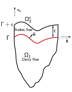
(a) Original Domain

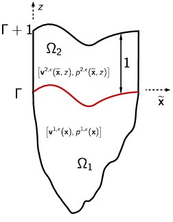
(b) Scaled Domain after the change of variable $\mathbf{x}\mapsto\varphi(\mathbf{x})$, with $\varphi$ defined in Equation (10).

Figure 1: Figure (a) depicts the original domain with a thin channel on top, where we set the Stokes flow. Figure (b) depicts the domain after scaling by the change of variables $\mathbf{x}\mapsto\varphi(\mathbf{x})$, where $\varphi$ is defined in Equation (10). This will be the domain of reference which is used for asymptotic analysis of the problem.

Notation

We shall use standard function spaces (see [20], [1]). For any smooth bounded region $G$ in $\bm{\mathbbm{R}}^{N}$ with boundary $\partial G$, the space of square integrable functions is denoted by $L^{2}(G)$, and the Sobolev space $H^{1}(G)$ consists of those functions in $L^{2}(G)$ for which each of the first-order weak partial derivatives belongs to $L^{2}(G)$. The trace is the continuous linear function $\gamma:H^{1}(G)\rightarrow L^{2}(\partial G)$ which agrees with restriction to the boundary on smooth functions, i.e., $\gamma(w)=w\big{|}_{\partial G}$ if $w\in C(\operatorname*{cl}(G))$. Its kernel is $H_{0}^{1}(G)\overset{\mathbf{def}}{=}\{w\in H^{1}(G):\gamma(w)=0\}$. The trace space is $H^{1/2}(\partial G)\overset{\mathbf{def}}{=}\gamma(H^{1}(G))$, the range of $\gamma$ endowed with the usual norm from the quotient space $H^{1}(G)/H_{0}^{1}(G)$, and we denote by $H^{-1/2}(\partial G)$ its topological dual. Column vectors and corresponding vector-valued functions will be denoted by boldface symbols, e.g., we denote the product space $\big{[}L^{2}(G)\big{]}^{N}$ by $\mathbf{L}^{2}(G)$ and the respective $N$-tuple of Sobolev spaces by $\mathbf{H}^{1}(G)\overset{\mathbf{def}}{=}\big{[}H^{1}(G)\big{]}^{N}$. Each $w\in H^{1}(G)$ has gradient $\bm{\nabla}w=\big{(}\frac{\partial w}{\partial x_{1}},\ldots,\frac{\partial w}{\partial x_{\scriptscriptstyle N}}\big{)}\in\mathbf{L}^{2}(G)$, furthermore we understand it as a row vector. We shall also use the space $\mathbf{H}_{\operatorname*{div}}(G)$ of vector functions $\mathbf{w}\in{\mathbf{L}}^{2}(G)$ whose weak divergence $\bm{\nabla\cdot}\mathbf{w}$ belongs to $L^{2}(G)$. Let $\bm{\widehat{n}}$ be the unit outward normal vector on $\partial G$. If $\mathbf{w}$ is a vector function on $\partial G$, we denote its normal component by $\mathbf{w}_{\,\bm{\widehat{n}}}=\gamma(\mathbf{w})\cdot\bm{\widehat{n}}$, its normal projection by $\mathbf{w}(\bm{\widehat{n}})=\mathbf{w}_{\,\bm{\widehat{n}}}\,\bm{\widehat{n}}$. The tangential component is $\mathbf{w}(\operatorname*{tg})=\mathbf{w}-\mathbf{w}(\bm{\widehat{n}})$. The notation $\mathbf{w}_{N},\mathbf{w}_{T}$ indicate respectively, the last component and the first $N-1$ components of the vector function $\mathbf{w}$ in the canonical basis. For the functions $\mathbf{w}\in\mathbf{H}_{\operatorname*{div}}(G)$, there is a normal trace defined on the boundary values, which will be denoted by $\mathbf{w}\cdot\bm{\widehat{n}}\in H^{-1/2}(\partial G)$. For those $\mathbf{w}\in\mathbf{H}^{1}(G)$ this agrees with $\gamma(\mathbf{w})\cdot\bm{\widehat{n}}$. Greek letters are used to denote general second-order tensors. The contraction of two tensors is given by $\sigma\bm{:}\kappa=\sum_{i,\,j}\,\sigma_{ij}\kappa_{ij}$. For a tensor-valued function $\kappa$ on $\partial G$, we denote the normal component (vector) by $\kappa(\bm{\widehat{n}})\overset{\mathbf{def}}{=}\sum_{j}\,\kappa_{ij}\,\bm{\widehat{n}}_{j}\in\bm{\mathbbm{R}}^{N}$, and its normal and tangential parts by $\kappa(\bm{\widehat{n}})\cdot\bm{\widehat{n}}=\kappa(\bm{\widehat{n}})_{\,\bm{\widehat{n}}}\overset{\mathbf{def}}{=}\sum_{i,\,j}\,\kappa_{ij}\bm{\widehat{n}}_{i}\bm{\widehat{n}}_{j}$ and $\kappa(\bm{\widehat{n}})_{\operatorname*{tg}}\overset{\mathbf{def}}{=}\kappa(\bm{\widehat{n}})-\kappa_{\,\bm{\widehat{n}}}\,\bm{\widehat{n}}$, respectively. For a vector function $\mathbf{w}\in\mathbf{H}^{1}(G)$, the tensor $(\bm{\nabla}\mathbf{w})_{ij}=\frac{\partial w_{i}}{\partial x_{j}}$ is the gradient of $\mathbf{w}$ and $\big{(}\bm{\mathcal{E}}(\mathbf{w})\big{)}_{ij}=\tfrac{1}{2}\big{(}\frac{\partial w_{i}}{\partial x_{j}}+\frac{\partial w_{j}}{\partial x_{i}}\big{)}$ is the symmetric gradient.

For a column vector $\mathbf{x}=\big{(}x_{\,1},\,\ldots,\,x_{\scriptscriptstyle N-1},\,x_{\scriptscriptstyle N}\big{)}\in\bm{\mathbbm{R}}^{N}$ we denote the corresponding vector in $\bm{\mathbbm{R}}^{N-1}$ consisting of the first $N-1$ components by $\widetilde{\mathbf{x}}=\big{(}x_{1},\,\ldots,\,x_{\scriptscriptstyle N-1}\big{)}$, and we identify $\bm{\mathbbm{R}}^{N-1}\times\{0\}$ with $\bm{\mathbbm{R}}^{N-1}$ by $\mathbf{x}=(\widetilde{\mathbf{x}},x_{\scriptscriptstyle N})$. The operators $\bm{\nabla}_{\!\!\scriptscriptstyle T}$, $\bm{\nabla}_{\!\!\scriptscriptstyle T}\bm{\cdot}$ denote respectively the $\bm{\mathbbm{R}}^{N-1}$-gradient and the $\bm{\mathbbm{R}}^{N-1}$-divergence in the first $N-1$-canonical directions, i.e. $\bm{\nabla}_{\!\!\scriptscriptstyle T}\overset{\mathbf{def}}{=}\big{(}\frac{\partial}{\partial x_{1}},\ldots,\frac{\partial}{\partial x_{\scriptscriptstyle N-1}}\big{)}$, $\bm{\nabla}_{\!\!\scriptscriptstyle T}\bm{\cdot}\overset{\mathbf{def}}{=}\big{(}\frac{\partial}{\partial x_{1}},\ldots,\frac{\partial}{\partial x_{\scriptscriptstyle N-1}}\big{)}$; moreover, we regard these operators as row vectors. Finally, $\bm{\nabla}^{t},\bm{\nabla}_{\!\!\scriptscriptstyle T}^{t}$ denote the same operators written as column vectors, i.e., the operators denoted as column vectors.

Remark 1

It shall be noticed that different notations have been chosen to indicate the first $N-1$ components: we use $\widetilde{\mathbf{x}}$ for a vector as variable $\mathbf{x}$, while we use $\mathbf{w}_{T}$ for a vector function $\mathbf{w}$ (or the operator $\bm{\nabla}_{\!\!\scriptscriptstyle T},\bm{\nabla}$ ). This difference in notation will ease keeping track of the involved variables and will not introduce confusion.

Preliminary Results

We close this section recalling some classic results.

Lemma 1

Let $G\subset\bm{\mathbbm{R}}^{N}$ be an open set with Lipschitz boundary, let $\bm{\widehat{n}}$ be the unit outward normal vector on $\partial G$. The normal trace operator $\mathbf{u}\in\mathbf{H}_{\operatorname*{div}}(G)\mapsto\mathbf{u}\cdot\bm{\widehat{n}}\in H^{-1/2}(\partial G)$ is defined by

$$\big{\langle}\mathbf{u}\cdot\bm{\widehat{n}},\phi\big{\rangle}_{\scriptscriptstyle H^{-1/2}(\partial G),\,H^{1/2}(\partial G)}\overset{\mathbf{def}}{=}\int_{G}\Big{(}\mathbf{u}\cdot\bm{\nabla}\phi+\bm{\nabla\cdot}\mathbf{u}\,\phi\Big{)}\,dx,\quad\phi\in H^{1}(G).$$ (1)

For any $g\in H^{-1/2}(\partial G)$ there exists $\mathbf{u}\in\mathbf{H}_{\operatorname*{div}}(G)$ such that $\mathbf{u}\cdot\bm{\widehat{n}}=g$ on $\partial G$ and $\|\mathbf{u}\|_{\mathbf{H}_{\operatorname*{div}}(G)}\leq K\|g\|_{H^{-1/2}(\partial G)}$, with $K$ depending only on the domain $G$. In particular, if $g$ belongs to $L^{2}(\partial G)$, the function $\mathbf{u}$ satisfies the estimate $\|\mathbf{u}\|_{\mathbf{H}_{\operatorname*{div}}(G)}\leq K\|g\|_{0,\partial G}$.

Proof 1

See Lemma 20.2 in [19].

Next we recall a central result to be used in this work

Theorem 2

Consider the problem a pair satisfying

$$\begin{split}(\mathbf{x},\mathbf{y})\in\mathbf{X}\times\mathbf{Y}:\quad{\mathcal{A}}\mathbf{x}+{\mathcal{B}}^{\prime}\mathbf{y}=F_{1}\quad\text{in}\;\mathbf{X}^{\prime},\\ -{\mathcal{B}}\mathbf{x}+{\mathcal{C}}\mathbf{y}=F_{2}\quad\text{in}\;\mathbf{Y}^{\prime}.\end{split}$$ (2)

Here $\mathbf{X},\mathbf{Y}$, $\mathbf{X}^{\prime},\mathbf{Y}^{\prime}$ are Hilbert spaces and their corresponding topological duals, $F_{1}\in\mathbf{X}^{\prime}$, $F_{2}\in\mathbf{Y}^{\prime}$ and the operators ${\mathcal{A}}:\mathbf{X}\rightarrow\mathbf{X}^{\prime}$, ${\mathcal{B}}:\mathbf{X}\rightarrow\mathbf{Y}^{\prime}$, ${\mathcal{C}}:\mathbf{Y}\rightarrow\mathbf{Y}^{\prime}$ are linear and continuous. Assume the operators satisfy

1. ${\mathcal{A}}$ is non-negative and $\mathbf{X}$-coercive on $\ker({\mathcal{B}})$,

2. ${\mathcal{B}}$ satisfies the inf-sup condition

   $$\inf_{\mathbf{y}\,\in\,\mathbf{Y}}\sup_{\mathbf{x}\,\in\,\mathbf{X}}\frac{|{\mathcal{B}}\mathbf{x}(\mathbf{y})|}{\|\mathbf{x}\|_{\mathbf{X}}\,\|\mathbf{y}\|_{\mathbf{Y}}}>0\,,$$ (3)

3. $C$ is non-negative and symmetric.

Then, for every $F_{1}\in\mathbf{X}^{\prime}$ and $F_{2}\in\mathbf{Y}^{\prime}$ the problem (2) has a unique solution $(\mathbf{x},\mathbf{y})\in\mathbf{X}\times\mathbf{Y}$, and it satisfies the estimate

$$\|\mathbf{x}\|_{\mathbf{X}}+\|\mathbf{y}\|_{\mathbf{Y}}\leq c\,(\|F_{1}\|_{\mathbf{X}^{\prime}}+\|F_{2}\|_{\mathbf{Y}^{\prime}})$$ (4)

for a positive constant $c$ depending only on the preceding assumptions on ${\mathcal{A}}$, ${\mathcal{B}}$, and ${\mathcal{C}}$.

Proof 2

See Section 4 in [10].

2 Geometric Setting and Formulation of the Problem

In this section we introduce the Darcy-Stokes coupled system analogous to the one presented in [14], for the case when the interface is curved. We begin with the geometric setting

2.1 Geometric Setting and Change of Coordinates

We describe here the geometry of the domains to be used in the present work; see Figure 1 (a) for the case $N=2$. The disjoint bounded domains $\Omega_{1}$ and $\Omega_{2}^{\epsilon}$ in $\bm{\mathbbm{R}}^{N}$ share the common interface, $\Gamma\overset{\mathbf{def}}{=}\partial\Omega_{1}\cap\partial\Omega_{2}^{\epsilon}\subseteq\bm{\mathbbm{R}}^{N}$, and we define $\Omega^{\epsilon}\overset{\mathbf{def}}{=}\Omega_{1}\cup\Gamma\cup\Omega_{2}^{\epsilon}$. The domain $\Omega_{1}$ is the porous medium, and $\Omega_{2}^{\epsilon}$ is the free fluid region. For simplicity we have assumed that the domain $\Omega_{2}^{\epsilon}$ is a cylinder defined by the interface $\Gamma$ and a small height $\epsilon>0$. It follows that the interface must verify specific requirements for a successful analysis

Hypothesis 1

There exists $G_{0},G$ bounded open connected domains $G_{0},G\subset\bm{\mathbbm{R}}^{N-1}$, such that $\operatorname*{cl}(G)\subset G_{0}$ and a $C^{2}(G_{0})$ function $\zeta:G_{0}\rightarrow\bm{\mathbbm{R}}$, such that the interface $\Gamma$ can be described by

$$\Gamma\overset{\mathbf{def}}{=}\big{\{}\big{(}\widetilde{\mathbf{x}},\,\zeta\,(\widetilde{\mathbf{x}})\big{)}:\,\widetilde{\mathbf{x}}\in G\,\big{\}},$$ (5)

i.e., $\Gamma$ is a $N-1$ manifold in $\bm{\mathbbm{R}}^{N}$. The domain $\Omega_{2}^{\epsilon}$ is described by

$$\Omega_{2}^{\epsilon}\overset{\mathbf{def}}{=}\big{\{}\big{(}\widetilde{\mathbf{x}},\,y\big{)}:\zeta\,(\widetilde{\mathbf{x}})<y<\zeta\,(\widetilde{\mathbf{x}})+\epsilon,\,\widetilde{\mathbf{x}}\in G\big{\}},$$ (6)

Remark 2

1. Observe that the domain $G$ is the orthogonal projection of the open surface $\Gamma\subseteq\bm{\mathbbm{R}}^{N}$ into $\bm{\mathbbm{R}}^{N-1}$.

2. Notice that due to the properties of $\zeta$ it must hold that if $\bm{\widehat{n}}=\bm{\widehat{n}}(\widetilde{\mathbf{x}})$ is the upwards unitary vector, orthogonal to the surface $\Gamma$ then

   $$\delta\overset{\mathbf{def}}{=}\inf\big{\{}\bm{\widehat{n}}(\widetilde{\mathbf{x}})\cdot\bm{\widehat{e}}_{N}:\widetilde{\mathbf{x}}\in G\big{\}}>0.$$ (7)

For simplicity of notation in the following we write

1. $$\Gamma+\epsilon\overset{\mathbf{def}}{=}\big{\{}\big{(}\widetilde{\mathbf{x}},\,\zeta\,(\widetilde{\mathbf{x}})+\epsilon\big{)}:\,\widetilde{\mathbf{x}}\in G\,\big{\}},$$ (8)

2. $$\Omega_{2}\overset{\mathbf{def}}{=}\Omega_{2}^{1}, \Omega\overset{\mathbf{def}}{=}\Omega^{1}.$$ (9)

For the asymptotic analysis of the coupled system, a domain of reference $\Omega$ will have to be fixed, see Figure 1 (b). Therefore we adopt a bijection between domains and account for the changes in the differential operators.

Definition 1

Let $\varphi:\Omega_{2}^{\epsilon}\rightarrow\Omega$ be the change of variables defined by

$$\varphi(y_{1},\ldots,y_{N-1},y_{N})\overset{\mathbf{def}}{=}\begin{Bmatrix}y_{1}\\ \vdots\\ y_{N-1}\\ \epsilon^{-1}\big{(}y_{N}-\zeta(y_{1},\ldots,y_{N-1})\big{)}+\zeta\big{(}y_{1},\ldots,y_{N-1}\big{)}\end{Bmatrix},$$ (10)

with $\mathbf{y}=\left(y_{1},\,\ldots,\,y_{N-1},\,y_{N}\right)\in\Omega_{2}^{\epsilon}$. Also, denote $\mathbf{x}=(x_{1},\ldots,x_{N-1},z)\overset{\mathbf{def}}{=}\varphi(\mathbf{y})$, i.e.

$$\mathbf{x}=(x_{1},\ldots,x_{N-1},z)\in\Omega_{2}, \mathbf{x}\cdot\bm{\widehat{e}}_{\ell}=\varphi(\mathbf{y})\cdot\bm{\widehat{e}}_{\ell}.$$ (11)

Remark 3

Observe that $\varphi:\Omega_{2}^{\epsilon}\rightarrow\Omega_{2}$ is a bijective map, see Figure 1 (b).

Gradient Operator

Denote by $\prescript{\mathbf{y}}{}{\bm{\nabla}},\prescript{\mathbf{x}}{}{\bm{\nabla}}$ the gradient operators with respect to the variables $\mathbf{y}$ and $\mathbf{x}$ respectively. Due to Definition 9 above, a direct computation shows that these operators satisfy the relationship

$$\prescript{\mathbf{y}}{}{\bm{\nabla}}^{t}=\begin{Bmatrix}\prescript{\mathbf{y}}{}{\bm{\nabla}_{\!\!\scriptscriptstyle T}}^{\!\!t}\\[3.0pt] \frac{\partial}{\partial y_{N}}\end{Bmatrix}=\begin{bmatrix}I&(1-\epsilon^{-1})\prescript{\mathbf{x}}{}{\bm{\nabla}_{\!\!\scriptscriptstyle T}}^{t}\zeta\\[3.0pt] \bm{0}&\epsilon^{-1}\end{bmatrix}\begin{Bmatrix}\prescript{\mathbf{x}}{}{\bm{\nabla}_{\!\!\scriptscriptstyle T}}^{t}\\[3.0pt] \partial_{z}\end{Bmatrix}.$$ (12)

In the block matrix notation above, it is understood that $I$ is the identity matrix in $\bm{\mathbbm{R}}^{(N-1)\times(N-1)}$, $\bm{\nabla}_{\!\!\scriptscriptstyle T}\zeta,\bm{0}$ are vectors in $\bm{\mathbbm{R}}^{N-1}$ and $\partial_{z}=\frac{\partial}{\partial z}$. In order to apply these changes to the gradient of a vector function $\mathbf{w}$, we recall the matrix notation

$$\prescript{\mathbf{y}}{}{\bm{\nabla}}\,\mathbf{w}=\begin{bmatrix}\prescript{\mathbf{y}}{}{\bm{\nabla}}w_{\scriptscriptstyle 1}\\ \vdots\\ \prescript{\mathbf{y}}{}{\bm{\nabla}}w_{\scriptscriptstyle N}\end{bmatrix}=\begin{bmatrix}\prescript{\mathbf{x}}{}{\bm{\nabla}_{\!\!\scriptscriptstyle T}}w_{1}+(1-\epsilon^{-1})\partial_{z}w_{1}\prescript{\mathbf{x}}{}{\bm{\nabla}_{\!\!\scriptscriptstyle T}}\zeta&\epsilon^{-1}\,\partial_{z}w_{1}\,\\ \vdots&\vdots\\ \prescript{\mathbf{x}}{}{\bm{\nabla}_{\!\!\scriptscriptstyle T}}w_{N}+(1-\epsilon^{-1})\partial_{z}w_{N}\prescript{\mathbf{x}}{}{\bm{\nabla}_{\!\!\scriptscriptstyle T}}\zeta&\epsilon^{-1}\,\partial_{z}w_{N}\,\end{bmatrix},$$ (13)

reordering we get

$$\prescript{\mathbf{y}}{}{\bm{\nabla}}\mathbf{w}\left(\widetilde{\mathbf{x}},\,x_{\scriptscriptstyle N}\right)=\begin{bmatrix}\prescript{\mathbf{x}}{}{\bm{D}}^{\epsilon}\mathbf{w}&\dfrac{1}{\epsilon}\,\partial_{z}\,\mathbf{w}\end{bmatrix}.$$ (14)

Here, the operator $\prescript{\mathbf{x}}{}{\bm{D}^{\epsilon}}$ is defined by

$$\prescript{\mathbf{x}}{}{\bm{D}^{\epsilon}}\mathbf{w}\overset{\mathbf{def}}{=}\prescript{\mathbf{x}}{}{\bm{\nabla}_{\!\!\scriptscriptstyle T}}\mathbf{w}+\Big{(}1-\frac{1}{\epsilon}\Big{)}\partial_{z}\mathbf{w}\prescript{\mathbf{x}}{}{\bm{\nabla}_{\!\!\scriptscriptstyle T}}^{t}\zeta,$$ (15)

i.e., $\prescript{\mathbf{x}}{}{\bm{D}^{\epsilon}}\,\mathbf{w}\in\bm{\mathbbm{R}}^{N\times(N-1)}$ and it is introduced to have a more efficient notation. In the next section we address the interface conditions.

Divergence Operator

Observing the diagonal of the matrix in (13) we have

$$\prescript{\mathbf{y}}{}{\bm{\nabla\cdot}}\,\mathbf{w}\,(\widetilde{\mathbf{x}},x_{\scriptscriptstyle N})=\Big{(}\prescript{\mathbf{x}}{}{\bm{\nabla}_{\!\!\scriptscriptstyle T}\bm{\cdot}}\,\mathbf{w}_{\scriptscriptstyle T}+\Big{(}1-\frac{1}{\epsilon}\Big{)}\partial_{z}\,\mathbf{w}_{\scriptscriptstyle T}\cdot\prescript{\mathbf{x}}{}{\bm{\nabla}_{\!\!\scriptscriptstyle T}\bm{\cdot}}\,\zeta\Big{)}(\widetilde{\mathbf{x}},z)+\frac{1}{\epsilon}\,\partial_{z}\mathbf{w}_{\scriptscriptstyle N}\left(\widetilde{\mathbf{x}},\,z\right)\\$$ (16)

Remark 4

The prescript indexes $\mathbf{y},\mathbf{x}$ written on the operators above were used only to derive the relation between them , however they will be dropped once the context is clear.

Local vs Global Vector Basis

It shall be seen later on, that the velocities of the channel need to be expressed in terms of an orthonormal basis ${\mathcal{B}}$, such that the normal vector $\bm{\widehat{n}}$ belongs to ${\mathcal{B}}$ and the remaining vectors are locally tangent to the interface $\Gamma$. Since $\zeta:G\rightarrow\bm{\mathbbm{R}}$ is a $C^{2}$ function it follows that $\widetilde{\mathbf{x}}\mapsto\bm{\widehat{n}}(\widetilde{\mathbf{x}})$ is at least $C^{1}$.

Definition 2

Let ${\mathcal{B}}_{0}\overset{\mathbf{def}}{=}\big{\{}\bm{\widehat{e}}_{1},\ldots,\bm{\widehat{e}}_{N-1},\bm{\widehat{e}}_{N}\big{\}}$ be the standard canonical basis in $\bm{\mathbbm{R}}^{N}$. For any $\widetilde{\mathbf{x}}\in G$ let ${\mathcal{B}}={\mathcal{B}}(\widetilde{\mathbf{x}})\overset{\mathbf{def}}{=}\big{\{}\bm{\widehat{\nu}}_{1},\ldots,\bm{\widehat{\nu}}_{N-1},\bm{\widehat{n}}\big{\}}$ be an orthonormal basis in $\bm{\mathbbm{R}}^{N}$. Define the linear map $U(\widetilde{\mathbf{x}}):\bm{\mathbbm{R}}^{N}\rightarrow\bm{\mathbbm{R}}^{N}$ by

$$U(\widetilde{\mathbf{x}})\bm{\widehat{\nu}}_{i}\overset{\mathbf{def}}{=}\bm{\widehat{e}}_{i},\text{ for }i=1,\ldots,N-1, U(\widetilde{\mathbf{x}})\bm{\widehat{n}}\overset{\mathbf{def}}{=}\bm{\widehat{e}}_{N}.$$ (17)

We say the map $\widetilde{\mathbf{x}}\mapsto U(\widetilde{\mathbf{x}})$ is a stream line localizer if it is of class $C^{1}$. In the sequel we write it with the following block matrix notation

$$U(\widetilde{\mathbf{x}})\overset{\mathbf{def}}{=}\begin{bmatrix}U^{T,\operatorname*{tg}}(\widetilde{\mathbf{x}})&U^{T,\bm{\widehat{n}}}(\widetilde{\mathbf{x}})\\ U^{N,\operatorname*{tg}}(\widetilde{\mathbf{x}})&U^{N,\bm{\widehat{n}}}(\widetilde{\mathbf{x}})\end{bmatrix}.$$ (18)

Here, the indexes $T$ and $N$ stands for the first $N-1$ components and the last component of the vector field. The indexes $\operatorname*{tg}$ and $\bm{\widehat{n}}$ indicate the tangent and normal directions to the interface $\Gamma$.

Remark 5

1. Since $\zeta\in C^{2}(G)$ and bounded, it is clear that for each $\widetilde{\mathbf{x}}\in G$ basis ${\mathcal{B}}=\big{\{}\bm{\widehat{\nu}}_{1},\ldots,\bm{\widehat{\nu}}_{N-1},\bm{\widehat{n}}\big{\}}$ can be chosen, so that $\widetilde{\mathbf{x}}\mapsto U(\widetilde{\mathbf{x}})$ is $C^{1}$. In the following it will be assumed that $U$ is a stream line localizer.

2. Notice that by definition $U(\widetilde{\mathbf{x}})$ is an orthogonal matrix for all $\widetilde{\mathbf{x}}\in G$.

Next, we express the velocities in the local basis $\mathbf{w}^{2}$ in terms of the normal and tangential components, using the following relations

$$\mathbf{w}_{\,\bm{\widehat{n}}(\widetilde{x}\,)}^{2}=\mathbf{w}^{2}\cdot\bm{\widehat{n}}(\widetilde{\mathbf{x}}),$$ (19a)

$$\mathbf{w}_{\,\operatorname*{tg}(\widetilde{x})}^{2}=\begin{Bmatrix}\mathbf{w}^{2}\cdot\bm{\widehat{\nu}}_{1}(\widetilde{\mathbf{x}})\\ \vdots\\ \mathbf{w}^{2}\cdot\bm{\widehat{\nu}}_{N-1}(\widetilde{\mathbf{x}})\end{Bmatrix}.$$ (19b)

Clearly, the relationship between velocities is given by

$$\mathbf{w}^{2}\big{(}\widetilde{\mathbf{x}},x_{\scriptscriptstyle N}\big{)}=U(\widetilde{\mathbf{x}})\begin{Bmatrix}\mathbf{w}_{\,\operatorname*{tg}(\widetilde{x})}^{2}\\[3.0pt] \mathbf{w}_{\,\bm{\widehat{n}}(\widetilde{x}\,)}^{2}\end{Bmatrix}\big{(}\widetilde{\mathbf{x}},x_{\scriptscriptstyle N}\big{)}\\ =\begin{bmatrix}U^{T,\operatorname*{tg}}(\widetilde{\mathbf{x}})&U^{T,\bm{\widehat{n}}}(\widetilde{\mathbf{x}})\\[3.0pt] U^{N,\operatorname*{tg}}(\widetilde{\mathbf{x}})&U^{N,\bm{\widehat{n}}}(\widetilde{\mathbf{x}})\end{bmatrix}\begin{Bmatrix}\mathbf{w}_{\,\operatorname*{tg}(\widetilde{x})}^{2}\\[3.0pt] \mathbf{w}_{\,\bm{\widehat{n}}(\widetilde{x}\,)}^{2}\end{Bmatrix}\big{(}\widetilde{\mathbf{x}},x_{\scriptscriptstyle N}\big{)}.$$ (20)

Remark 6

We stress the following observations

1. The procedure above does not modify the dependence of the variables, only the way velocity field are expressed as linear combinations of a convenient (stream line) orthonormal basis.

2. The fact that $U$ is a smooth function allows to claim that $\mathbf{w}_{\,\operatorname*{tg}}^{2}\in\big{[}H^{1}(\Omega_{2})\big{]}^{N-1}$ and $\mathbf{w}_{\,\bm{\widehat{n}}}^{2}\in H^{1}(\Omega_{2})$.

3. In order to keep notation as light as possible the dependence of the matrix $U$ as well as the normal and tangential directions $\bm{\widehat{n}},\operatorname*{tg}$ will be omitted whenever is not necessary to show it.

4. Notice that given any two flow fields $\mathbf{u}^{2},\mathbf{w}^{2}$ the following isometric identities hold

   $$\begin{split}\mathbf{u}^{2}_{\operatorname*{tg}}\cdot\mathbf{w}^{2}_{\operatorname*{tg}}&=\mathbf{u}^{2}(\operatorname*{tg})\cdot\mathbf{w}^{2}(\operatorname*{tg}),\\ \mathbf{u}^{2}_{\bm{\widehat{n}}}\mathbf{w}^{2}_{\bm{\widehat{n}}}&=\mathbf{u}^{2}(\bm{\widehat{n}})\cdot\mathbf{w}^{2}(\bm{\widehat{n}}),\\ \mathbf{u}^{2}\cdot\mathbf{w}^{2}&=\mathbf{u}^{2}(\operatorname*{tg})\cdot\mathbf{w}^{2}(\operatorname*{tg})+\mathbf{u}^{2}(\bm{\widehat{n}})\cdot\mathbf{w}^{2}(\bm{\widehat{n}})=\mathbf{u}^{2}_{\operatorname*{tg}}\cdot\mathbf{w}^{2}_{\operatorname*{tg}}+\mathbf{u}^{2}_{\bm{\widehat{n}}}\mathbf{w}^{2}_{\bm{\widehat{n}}}.\end{split}$$ (21)

Proposition 3

Let $\mathbf{w}^{2}\in\mathbf{H}^{1}(\Omega_{2})$ and let $\mathbf{w}_{\,\bm{\widehat{n}}}^{2},\mathbf{w}_{\,\operatorname*{tg}}^{2}$ be as defined in (19), then

1. $$\partial_{z}\mathbf{w}^{2}\big{(}\widetilde{\mathbf{x}},x_{\scriptscriptstyle N}\big{)}=U(\widetilde{\mathbf{x}})\begin{Bmatrix}\partial_{z}\,\mathbf{w}_{\,\operatorname*{tg}(\widetilde{x})}^{2}\\[3.0pt] \partial_{z}\,\mathbf{w}_{\,\bm{\widehat{n}}(\widetilde{x}\,)}^{2}\end{Bmatrix}\big{(}\widetilde{\mathbf{x}},x_{\scriptscriptstyle N}\big{)}.$$ (22)

2. $$\big{\|}\partial_{z}\mathbf{w}^{2}\big{\|}^{2}_{0,\Omega_{2}}=\big{\|}\partial_{z}\mathbf{w}_{\scriptscriptstyle T}^{2}\big{\|}^{2}_{0,\Omega_{2}}+\big{\|}\partial_{z}\mathbf{w}_{\scriptscriptstyle N}^{2}\big{\|}^{2}_{0,\Omega_{2}}\\ =\big{\|}\partial_{z}\mathbf{w}_{\,\operatorname*{tg}}^{2}\big{\|}^{2}_{0,\Omega_{2}}+\big{\|}\partial_{z}\mathbf{w}_{\,\bm{\widehat{n}}}^{2}\big{\|}^{2}_{0,\Omega_{2}}.$$ (23)

Proof 3

1. It suffices to observe that the orthogonal matrix $U$ defined in (20) is independent from $z$.

2. Due to (22) we have

   $$\begin{split}\big{|}\partial_{z}\mathbf{w}^{2}\left(\widetilde{\mathbf{x}},x_{\scriptscriptstyle N}\right)\big{|}^{2}&=\partial_{z}\mathbf{w}^{2}\left(\widetilde{\mathbf{x}},x_{\scriptscriptstyle N}\right)\cdot\partial_{z}\mathbf{w}^{2}\left(\widetilde{\mathbf{x}},x_{\scriptscriptstyle N}\right)\\ &=U(\widetilde{\mathbf{x}})\begin{Bmatrix}\partial_{z}\,\mathbf{w}_{\,\operatorname*{tg}(\widetilde{x})}^{2}\\ \partial_{z}\,\mathbf{w}_{\,\bm{\widehat{n}}(\widetilde{x}\,)}^{2}\end{Bmatrix}\left(\widetilde{\mathbf{x}},x_{\scriptscriptstyle N}\right)\cdot U(\widetilde{\mathbf{x}})\begin{Bmatrix}\partial_{z}\,\mathbf{w}_{\,\operatorname*{tg}(\widetilde{x})}^{2}\\ \partial_{z}\,\mathbf{w}_{\,\bm{\widehat{n}}(\widetilde{x}\,)}^{2}\end{Bmatrix}\left(\widetilde{\mathbf{x}},x_{\scriptscriptstyle N}\right)\\ &=\bigg{|}\begin{Bmatrix}\partial_{z}\,\mathbf{w}_{\,\operatorname*{tg}(\widetilde{x})}^{2}\\ \partial_{z}\,\mathbf{w}_{\,\bm{\widehat{n}}(\widetilde{x}\,)}^{2}\end{Bmatrix}\bigg{|}^{2}.\end{split}$$

   The last equality holds true since the matrix $U(\widetilde{\mathbf{x}})$ is orthogonal at each point $\widetilde{\mathbf{x}}\in G$, therefore it is an isometry in the Hilbert space $\big{(}\bm{\mathbbm{R}}^{N},\cdot\big{)}$. Recalling that $\big{|}\partial_{z}\mathbf{w}_{\scriptscriptstyle T}^{2}\big{(}\widetilde{\mathbf{x}},x_{\scriptscriptstyle N}\big{)}\big{|}^{2}+\big{|}\partial_{z}\mathbf{w}_{\scriptscriptstyle N}^{2}\big{(}\widetilde{\mathbf{x}},x_{\scriptscriptstyle N}\big{)}\big{|}^{2}=\big{|}\partial_{z}\mathbf{w}^{2}\big{(}\widetilde{\mathbf{x}},x_{\scriptscriptstyle N}\big{)}\big{|}^{2}$ for all $\mathbf{x}=(\widetilde{\mathbf{x}},x_{\scriptscriptstyle N})$, the result follows.

2.2 Interface Conditions and the Strong Form

The interface conditions need to account for stress and mass balance. We start with the stress, to that end we decompose it in the tangential and normal components, the former is handled by the Beavers-Joseph-Saffman (24a) condition and the latter by the classical Robin boundary condition (24b), this gives

$$\sigma^{2}(\bm{\widehat{n}})_{\operatorname*{tg}}=\epsilon^{2}\,\beta\,\sqrt{{\mathcal{Q}}}\,\mathbf{v}^{2}(\operatorname*{tg})\,,$$ (24a)

$$\sigma^{2}(\bm{\widehat{n}})_{\bm{\widehat{n}}}-p^{2}+p^{1}=\alpha\,\mathbf{v}^{1}\cdot\bm{\widehat{n}}\text{ on }\Gamma.$$ (24b)

In the expression (24a) above, $\epsilon^{2}$ is a scaling factor destined to balance out the geometric singularity introduced by the thinness of the channel. In addition, the coefficient $\alpha\geq 0$ in (24b) is the fluid entry resistance.

Next, recall that the stress satisfies $\sigma^{2}=2\,\epsilon\,\mu\,\bm{\mathcal{E}}(\mathbf{v}^{2})$ (where the scale $\epsilon$ is introduced according to the thinness of the channel) and that $\bm{\nabla}\cdot\mathbf{v}^{2}=0$ (since the system is conservative); then we have

$$\bm{\nabla}\cdot\sigma^{2}=\bm{\nabla}\cdot\big{[}2\,\epsilon\,\mu\,\bm{\mathcal{E}}\big{(}\mathbf{v}^{2}\big{)}\big{]}=\epsilon\,\mu\bm{\nabla}\cdot\bm{\nabla}\mathbf{v}^{2}.$$

Replacing in the equations (24) we have the following set of interface conditions

$$\epsilon\,\mu\,\Big{(}\frac{\partial\,\mathbf{v}^{2}}{\partial\,\bm{\widehat{n}}}-\big{(}\frac{\partial\,\mathbf{v}^{2}}{\partial\,\bm{\widehat{n}}}\cdot\bm{\widehat{n}}\big{)}\bm{\widehat{n}}\Big{)}=\epsilon^{2}\beta\,\sqrt{{\mathcal{Q}}}\,\mathbf{v}^{2}(\operatorname*{tg})\,,$$ (25a)

$$\epsilon\,\mu\Big{(}\frac{\partial\,\mathbf{v}^{2}}{\partial\,\bm{\widehat{n}}}\cdot\bm{\widehat{n}}\Big{)}-p^{2}+p^{1}=\alpha\,\mathbf{v}^{1}\cdot\bm{\widehat{n}}\text{ on }\Gamma.$$ (25b)

$$\mathbf{v}^{1}\cdot\bm{\widehat{n}}=\mathbf{v}^{2}\cdot\bm{\widehat{n}}\text{ on }\Gamma.$$ (25c)

The condition (25c) states the fluid flow (or mass) balance.

With the previous considerations, the Darcy-Stokes coupled system in terms of velocity $\mathbf{v}$ and pressure $p$ is given by

$$\bm{\nabla\cdot}\mathbf{v}^{1}=h_{1}\,,$$ (26a)

$${\mathcal{Q}}\,\mathbf{v}^{1}+\bm{\nabla}p^{1}=\mathbf{0}\,,\quad\text{in }\Omega_{1}.$$ (26b)

$$\bm{\nabla}\cdot\mathbf{v}^{2}=0,$$ (26c)

$$-\bm{\nabla}\cdot 2\epsilon\mu\bm{\mathcal{E}}(\mathbf{v}^{2})+\bm{\nabla}p^{2}=\mathbf{f}_{2}.$$ (26d)

Here, equations (26a), (26b) correspond to the Darcy flow filtration through the porous medium, while equations (26c) and (26d) stand for the Stokes free flow. Finally, we adopt the following boundary conditions

$$p^{1}=0\,\quad\text{on }\,\partial\Omega_{1}-\Gamma.$$ (27a)

$$\mathbf{v}^{2}=0\,\quad\text{on }\,\partial\Omega_{2}^{\epsilon}-\big{(}\Gamma+\epsilon\big{)}.$$ (27b)

$$\frac{\partial\,\mathbf{v}^{2}}{\partial\,\bm{\widehat{n}}}-\Big{(}\frac{\partial\,\mathbf{v}^{2}}{\partial\,\bm{\widehat{n}}}\cdot\bm{\widehat{n}}\Big{)}\bm{\widehat{n}}=0\quad\text{on}\;\Gamma+\epsilon,$$ (27c)

$$\mathbf{v}^{2}\cdot\bm{\widehat{n}}=\mathbf{v}_{\,\bm{\widehat{n}}}^{\,2}=0\quad\text{on}\;\Gamma+\epsilon.$$ (27d)

The system of equations (26), (27) and (25) constitute the strong form of the Darcy-Stokes coupled system.

Remark 7

1. For a detailed exposition on the system’s adopted scaling namely, the fluid stress tensor $\sigma^{2}=2\,\epsilon\,\mu\,\bm{\mathcal{E}}(\mathbf{v}^{2})$ and the Beavers-Joseph-Saffman condition (24a), together with the formal asymptotic analysis we refer to [15].

2. A deep discussion on the role of each physical variable and parameter in equations (26) as well as the meaning of the boundary conditions (27), can be found in Sections 1.2, 1.3 and 1.4 in [14].

2.3 Weak Variational Formulation and a Reference Domain

In this section we present the weak variational formulation of the problem defined by the system of equations (26), (27) and (25), on the domain $\Omega^{\epsilon}$, next, we rescale $\Omega_{2}^{\epsilon}$ to get a uniform domain of reference. We begin defining the function spaces where the problem is modeled

Definition 3

Let $\Omega,\Omega_{1},\Omega_{2}^{\epsilon},\Gamma$ be as introduced in Section 2.1; in particular $\Omega_{2}$ and $\Gamma$ satisfy Hypothesis 1. Define the spaces

$$\mathbf{X}_{2}^{\epsilon}\overset{\mathbf{def}}{=}\big{\{}\mathbf{v}\in\mathbf{H^{1}}(\Omega_{2}^{\epsilon}):\mathbf{v}=0\text{ on }\partial\Omega_{2}^{\epsilon}-\big{(}\Gamma+\epsilon\big{)},\;\mathbf{v}\cdot\bm{\widehat{n}}=0\;\text{on}\,\Gamma+\epsilon\,\big{\}},$$ (28a)

$$\mathbf{X}^{\epsilon}\overset{\mathbf{def}}{=}\big{\{}[\,\mathbf{v}^{1},\mathbf{v}^{2}\,]\in\mathbf{H}_{\operatorname*{div}}(\Omega_{1}^{\epsilon})\times\mathbf{X}_{2}^{\epsilon}:\mathbf{v}^{1}\cdot\bm{\widehat{n}}=\mathbf{v}^{2}\cdot\bm{\widehat{n}}\;\text{on}\,\Gamma\big{\}}=\big{\{}\mathbf{v}\in\mathbf{H}_{\operatorname*{div}}(\Omega^{\epsilon}):\mathbf{v}^{2}\in\mathbf{X}_{2}^{\epsilon}\big{\}},$$ (28b)

$$\mathbf{Y}^{\epsilon}\overset{\mathbf{def}}{=}L^{2}(\Omega^{\epsilon}),$$ (28c)

endowed with their respective natural norms. Moreover, for $\epsilon=1$ we simply write $\mathbf{X}$, $\mathbf{X}_{2}$ and $\mathbf{Y}$.

In order to attain well-posedness of the problem, the following hypothesis is adopted.

Hypothesis 2

It will be assumed that $\mu>0$ and the coefficients $\beta$ and $\alpha$ are nonnegative and bounded almost everywhere. Moreover, the tensor ${\mathcal{Q}}$ is elliptic, i.e., there exists a $C_{{\mathcal{Q}}}>0$ such that $({\mathcal{Q}}\,\mathbf{x})\cdot\mathbf{x}\geq C_{{\mathcal{Q}}}\|\mathbf{x}\|^{2}$ for all $\mathbf{x}\in\bm{\mathbbm{R}}^{N}$.

Theorem 4

Consider the boundary-value problem defined by the equations (26), the interface coupling conditions (25) and the boundary conditions (27) then

1. A weak variational formulation of the problem is given by

   $$\big{[}\,\mathbf{v}^{\epsilon},p^{\epsilon}\,\big{]}\in\mathbf{X}^{\epsilon}\times\mathbf{Y}^{\epsilon}:$$

   $$\int_{\Omega_{1}}\big{(}{\mathcal{Q}}\,\mathbf{v}^{1,\,\epsilon}\cdot\mathbf{w}^{1} -p^{1,\epsilon}\,\bm{\nabla}\cdot\mathbf{w}^{1}\big{)}\,d\mathbf{y}+\int_{\Omega_{2}^{\epsilon}}\big{(}\,\epsilon\,\mu\bm{\nabla}\,\mathbf{v}^{\,2,\epsilon}-p^{\,2,\epsilon}\delta\ \big{)}\bm{:}\bm{\nabla}\mathbf{w}^{2}\,d\widetilde{\mathbf{y}}d\mathbf{y}_{\scriptscriptstyle N}$$ (29a)

   $$+\,\alpha\int_{\Gamma}\big{(}\mathbf{v}^{\,2,\epsilon}\,\cdot\bm{\widehat{n}}\big{)}\, \big{(}\mathbf{w}^{2}\cdot\bm{\widehat{n}}\big{)}\,dS+\int_{\Gamma}\epsilon^{2}\,\beta\,\sqrt{{\mathcal{Q}}}\;\mathbf{v}_{\,\operatorname*{tg}}^{2,\epsilon}\cdot\mathbf{w}_{\,\operatorname*{tg}}^{2}\,dS=\int_{\Omega_{2}^{\epsilon}}{\mathbf{f}^{\,2,\,\epsilon}}\cdot\mathbf{w}^{2}\,d\widetilde{\mathbf{y}}\,d\mathbf{y}_{\scriptscriptstyle N},$$

   $$\int_{\Omega_{1}}\bm{\nabla}\cdot\mathbf{v}^{1,\epsilon}\,\varphi^{1}\,d\mathbf{y} +\int_{\Omega_{2}^{\epsilon}}\bm{\nabla}\cdot\mathbf{v}^{\,2,\epsilon}\,\varphi^{2}\,d\widetilde{\mathbf{y}}\,d\mathbf{y}_{\scriptscriptstyle N}=\int_{\Omega_{1}}h^{1,\,\epsilon}\,\varphi^{1}\,d\mathbf{y},$$ (29b)

   for all $$\big{[}\mathbf{w},\varphi\big{]}\in\mathbf{X}^{\epsilon}\times\mathbf{Y}^{\epsilon}$$.

2. The problem (29) is well-posed.

3. The problem (29) is equivalent to

   $$[\mathbf{v}^{\,\epsilon},\mathbf{p}^{\,\epsilon}]\in\mathbf{X}\times\mathbf{Y}:$$

   $$\int_{\Omega_{1}}{\mathcal{Q}}\,\mathbf{v}^{1,\epsilon}\cdot\mathbf{w}^{1}\,d\mathbf{x}-\int_{\Omega_{1}}p^{1,\epsilon}\,\bm{\nabla\cdot}\mathbf{w}^{1}\,d\mathbf{x}\\ -\epsilon\int_{\Omega_{2}}p^{\,2,\epsilon}\,\bm{\nabla}_{\!\!\scriptscriptstyle T}\bm{\cdot}\mathbf{w}_{\scriptscriptstyle T}^{2}\,d\widetilde{\mathbf{x}}\,dz-\epsilon\Big{(}1-\frac{1}{\epsilon}\Big{)}\int_{\Omega_{2}}p^{\,2,\epsilon}\,\partial_{z}\,\mathbf{w}_{\scriptscriptstyle T}^{2}\cdot\bm{\nabla}_{\!\!\scriptscriptstyle T}\zeta\,d\widetilde{\mathbf{x}}\,dz-\int_{\Omega_{2}}p^{\,2,\epsilon}\,\partial_{z}\mathbf{w}_{\scriptscriptstyle N}^{2}\,d\widetilde{\mathbf{x}}\,dz\\ +\epsilon^{2}\int_{\Omega_{2}}\mu\,\bm{D}^{\epsilon}\mathbf{v}^{\,2,\epsilon}\bm{:}\bm{D}^{\epsilon}\mathbf{w}^{2}\,d\widetilde{\mathbf{x}}\,dz+\int_{\Omega_{2}}\mu\,\partial_{z}\,\mathbf{v}_{\scriptscriptstyle T}^{\,2,\epsilon}\cdot\partial_{z}\,\mathbf{w}_{\scriptscriptstyle T}^{2}\,d\widetilde{\mathbf{x}}\,dz+\int_{\Omega_{2}}\mu\,\partial_{z}\,\mathbf{v}_{\scriptscriptstyle N}^{\,2,\epsilon}\cdot\partial_{z}\,\mathbf{w}_{\scriptscriptstyle N}^{2}\,d\widetilde{\mathbf{x}}\,dz\\ +\alpha\int_{\Gamma}\big{(}\mathbf{v}^{1,\epsilon}\cdot\bm{\widehat{n}}\big{)}\,\big{(}\mathbf{w}^{1}\,\cdot\bm{\widehat{n}}\big{)}\,dS+\epsilon^{2}\int_{\Gamma}\beta\sqrt{{\mathcal{Q}}}\,\mathbf{v}_{\,\operatorname*{tg}}^{2,\epsilon}\cdot\mathbf{w}_{\,\operatorname*{tg}}^{2}\,dS=\epsilon\,\int_{\Omega_{2}}{\mathbf{f}^{2,\epsilon}}\cdot\mathbf{w}^{2}\,d\widetilde{\mathbf{x}}\,dz,$$ (30a)

   $$\int_{\Omega_{1}}\bm{\nabla\cdot}\mathbf{v}^{1,\epsilon}\varphi^{1}\,d\mathbf{x}+\epsilon\int_{\Omega_{2}}\bm{\nabla}_{\!\!\scriptscriptstyle T}\bm{\cdot}\mathbf{v}_{\scriptscriptstyle T}^{\,2,\epsilon}\,\varphi^{2}\,d\widetilde{\mathbf{x}}\,dz+\epsilon\Big{(}1-\frac{1}{\epsilon}\Big{)}\int_{\Omega_{2}}\partial_{z}\mathbf{v}_{\scriptscriptstyle T}^{\,2,\epsilon}\cdot\bm{\nabla}_{\!\!\scriptscriptstyle T}\zeta\,\varphi^{2}\,d\widetilde{\mathbf{x}}\,dz\\ +\int_{\Omega_{2}}\partial_{z}\mathbf{v}_{\scriptscriptstyle N}^{\,2,\epsilon}\,\varphi^{2}\,d\widetilde{\mathbf{x}}\,dz=\int_{\Omega_{1}}h^{1,\,\epsilon}\,\varphi^{1}\,d\mathbf{x},$$ (30b)

   $$\text{for all }[\mathbf{w},\Phi]\in\mathbf{X}\times\mathbf{Y}$$.

Proof 4

1. See Proposition 3 in [14], we simply highlight that the term $\int_{\Omega_{2}}\epsilon^{2}\beta\sqrt{{\mathcal{Q}}}\,\mathbf{v}^{2}(\operatorname*{tg})\cdot\mathbf{w}^{2}(\operatorname*{tg})\,dS$ has been replaced by $\int_{\Omega_{2}}\epsilon^{2}\beta\sqrt{{\mathcal{Q}}}\,\mathbf{v}_{\operatorname*{tg}}^{\,2}\cdot\mathbf{w}_{\,\operatorname*{tg}}^{2}\,dS$, due to the isometric identities (21).

2. See Theorem 6 in [14]. The technique identifies the operators ${\mathcal{A}},{\mathcal{B}},{\mathcal{C}}$ in the variational statements (29a) and (29b), then it verifies that these operators satisfy the hypotheses of Theorem 2; the result delivers well-posedness.

3. A direct substitution of the expressions (14) and (16) in the statements (29), combined with the definition (15) yields the result. Also notice that the determinant of the matrix in the right hand side of the equation (14) is equal to $\epsilon^{-1}$. Finally, observe that the boundary conditions of space $\mathbf{X}_{2}^{\epsilon}$, defined in (28a) are transformed into the boundary conditions of $\mathbf{X}_{2}$ because none of them involve derivatives.

Remark 8

In order to prevent heavy notation, from now on, we denote the volume integrals by $\int_{\Omega_{1}}F=\int_{\Omega_{1}}F\,d\mathbf{x}$ and $\int_{\Omega_{2}}F=\int_{\Omega_{2}}F\,d\widetilde{\mathbf{x}}\,dz$. We will use the explicit notation $\int_{\Omega_{2}}F\,d\widetilde{\mathbf{x}}\,dz$ only for those cases where specific calculations are needed. Both notations will be clear from the context.

3 Asymptotic Analysis

In this section, we present the asymptotic analysis of the problem i.e., we obtain a-priori estimates for the solutions $\big{(}(\mathbf{v}^{\,\epsilon},p^{\,\epsilon}):\epsilon>0\big{)}$, derive weak limits and conclude features about those (velocity and pressure) limits. We start recalling a classical space.

Definition 4

Let $\Omega_{2}$ as in Definition 1 and define the Hilbert space

$$H(\partial_{z},\Omega_{2}) \overset{\mathbf{def}}{=}\big{\{}w\in L^{2}(\Omega_{2}):\partial_{z}\,w\in\,L^{2}(\Omega_{2})\big{\}},$$ (31a)

$$\mathbf{H}(\partial_{z},\Omega_{2}) \overset{\mathbf{def}}{=}\big{\{}\mathbf{w}\in L^{2}(\Omega_{2}):\partial_{z}\,\mathbf{w}\in\,L^{2}(\Omega_{2})\big{\}},$$ (31b)

endowed with its natural inner product

Lemma 5

1. Let $H(\partial_{z},\Omega_{2})$ be the space introduced in Definition 4, then the trace map $w\mapsto w\big{|}_{\Gamma}$ from $H(\partial_{z},\Omega_{2})$ to $L^{2}(\Gamma)$ is well-defined. Moreover, the following Poincaré-type inequalities hold in this space

   $$\|w\|_{0,\Gamma}\;\leq\sqrt{2}\,\Big{(}\|w\|_{0,\Omega_{2}}+\|\partial_{z}\,w\|_{0,\Omega_{2}}\Big{)},$$ (32a)

   $$\|w\|_{0,\Omega_{2}}\;\leq\sqrt{2}\,\Big{(}\|\partial_{z}\,w\|_{0,\Omega_{2}}+\|w\|_{0,\Gamma}\Big{)},$$ (32b)

   for all $w\in H(\partial_{z},\Omega_{2})$.

2. Let $\mathbf{H}(\partial_{z},\Omega_{2})$ be the vector space introduced in Definition 4 then, for any $\mathbf{w}\in\mathbf{H}(\partial_{z},\Omega_{2})$ the estimates analogous to (32b) hold.

3. Let $\mathbf{w}^{2}\in\mathbf{H}^{1}(\Omega_{2})\subset\mathbf{H}(\partial_{z},\Omega_{2})$ and let $\mathbf{w}_{\,\bm{\widehat{n}}}^{2},\mathbf{w}_{\,\operatorname*{tg}}^{2}$ be as defined in (19), then

   $$\big{\|}\,\mathbf{w}_{\,\bm{\widehat{n}}}^{2}\,\big{\|}_{0,\Omega_{2}}\;\leq\big{\|}\,\partial_{z}\,\mathbf{w}_{\,\bm{\widehat{n}}}^{2}\,\big{\|}_{0,\Omega_{2}}+2\,\|\,\mathbf{w}_{\,\bm{\widehat{n}}}^{2}\,\|_{0,\Gamma},$$ (33a)

   $$\big{\|}\,\mathbf{w}_{\,\operatorname*{tg}}^{2}\,\big{\|}_{0,\Omega_{2}}\;\leq\big{\|}\,\partial_{z}\,\mathbf{w}_{\,\operatorname*{tg}}^{2}\,\big{\|}_{0,\Omega_{2}}+2\,\|\,\mathbf{w}_{\,\operatorname*{tg}}^{2}\,\|_{0,\Gamma}.$$ (33b)

Proof 5

1. The proof is a direct application of the fundamental theorem of calculus on the smooth functions $C^{\infty}(\Omega_{2})$ which is a dense subspace in $H(\partial_{z},\Omega_{2})$.

2. A direct application of equations (32) on each coordinate of $\mathbf{w}\in\mathbf{H}(\partial_{z},\Omega_{2})$ delivers the result.

3. It follows from a direct application of (i) and (ii) on $\mathbf{w}_{\,\bm{\widehat{n}}}^{2}$, $\mathbf{w}_{\,\operatorname*{tg}}^{2}$ respectively.

Next we show that the sequence of solutions is globally bounded under the following hypotheses.

Hypothesis 3

In the following, it will be assumed that the sequences $(\mathbf{f}^{2,\epsilon}:\epsilon>0)\subseteq\mathbf{L}^{2}(\Omega_{2})$ and $(h^{1,\epsilon}:\epsilon>0)\subseteq L^{2}(\Omega_{1})$ are bounded, i.e., there exists $C>0$ such that

$$\big{\|}\mathbf{f}^{2,\epsilon}\big{\|}_{0,\Omega_{2}}\leq C, \big{\|}h^{1,\epsilon}\big{\|}_{0,\Omega_{1}}\leq C, \text{for all }\,\epsilon>0.$$ (34)

Theorem 6 (Global a-priori Estimate)

Let $[\mathbf{v}^{\,\epsilon},p^{\,\epsilon}]\in\mathbf{X}\times\mathbf{Y}$ be the solution to the Problem (30). There exists a constant $K>0$ such that

$$\big{\|}\mathbf{v}^{1,\epsilon}\big{\|}_{0,\Omega_{1}}^{2}+\big{\|}\,\bm{D}^{\epsilon}\big{(}\,\epsilon\,\mathbf{v}^{\,2,\epsilon}\,\big{)}\big{\|}_{0,\Omega_{2}}^{2}+\big{\|}\partial_{z}\mathbf{v}_{\scriptscriptstyle T}^{\,2,\epsilon}\big{\|}_{0,\Omega_{2}}^{2}+\big{\|}\partial_{z}\mathbf{v}_{\scriptscriptstyle N}^{\,2,\epsilon}\big{\|}_{0,\Omega_{2}}^{2}+\big{\|}\mathbf{v}_{\,\bm{\widehat{n}}}^{2,\epsilon}\big{\|}_{0,\Gamma}^{2}+\big{\|}\epsilon\,\mathbf{v}_{\,\operatorname*{tg}}^{2,\epsilon}\big{\|}_{0,\Gamma}^{2}\leq K, \text{for all }\,\epsilon>0.$$ (35)

Proof 6

Set $\mathbf{w}=\mathbf{v}^{\epsilon}$ in (30a) and $\varphi=p^{\epsilon}$ in (30b) and add them together. In addition, apply the Cauchy-Bunyakowsky-Schwartz inequality to the right hand side and recall the Hypothesis 2, this gives

$$\big{\|}\,\mathbf{v}^{1,\epsilon}\,\big{\|}_{0,\Omega_{1}}^{2}+\epsilon^{\,2}\int_{\Omega_{2}}\bm{D}^{\epsilon}\,\mathbf{v}^{\,2,\epsilon}:\bm{D}^{\epsilon}\,\mathbf{v}^{\,2,\epsilon}+\big{\|}\,\partial_{z}\mathbf{v}_{\scriptscriptstyle T}^{\,2,\epsilon}\,\big{\|}_{0,\Omega_{2}}^{2}+\big{\|}\,\partial_{z}\mathbf{v}_{\scriptscriptstyle N}^{\,2,\epsilon}\,\big{\|}_{0,\Omega_{2}}^{2}+\,\big{\|}\,\mathbf{v}^{1,\epsilon}\cdot\bm{\widehat{n}}\,\big{\|}_{0,\Gamma}^{2}+\big{\|}\,\epsilon\,\mathbf{v}_{\,\operatorname*{tg}}^{2,\epsilon}\,\big{\|}_{0,\Gamma}^{2}\\ \leq\frac{1}{k}\Big{(}\big{\|}\mathbf{f}^{2,\epsilon}_{\tau}\big{\|}_{0,\Omega_{2}}\big{\|}\big{(}\epsilon\,\mathbf{v}_{\,\operatorname*{tg}}^{2,\epsilon}\big{)}\big{\|}_{0,\Omega_{2}}+\big{\|}\mathbf{f}^{2,\epsilon}_{\bm{\widehat{n}}}\big{\|}_{0,\Omega_{2}}\big{\|}\big{(}\epsilon\,\mathbf{v}_{\,\bm{\widehat{n}}}^{2,\epsilon}\big{)}\big{\|}_{0,\Omega_{2}}+\int_{\Omega_{1}}h^{1,\,\epsilon}\,p^{1,\epsilon}\,dx\,\Big{)}.$$ (36)

The mixed terms were canceled out on the diagonal. We focus on the summand involving an integral in the right hand side of the expression above, i.e.,

$$\begin{split}\int_{\Omega_{1}}h^{1,\epsilon}\,p^{1,\epsilon}\,dx&\leq\big{\|}\,p^{1,\epsilon}\,\big{\|}_{0,\Omega_{1}}\big{\|}\,h^{1,\epsilon}\,\big{\|}_{0,\Omega_{1}}\\ &\leq C\big{\|}\,\bm{\nabla}p^{1,\epsilon}\,\big{\|}_{0,\Omega_{1}}\big{\|}\,h^{1,\epsilon}\,\big{\|}_{0,\Omega_{1}}=\big{\|}\,{\mathcal{Q}}\,\mathbf{v}^{1,\epsilon}\,\big{\|}_{0,\Omega_{1}}\big{\|}\,h^{1,\epsilon}\,\big{\|}_{0,\Omega_{1}}\leq\widetilde{C}\big{\|}\,\mathbf{v}^{1,\epsilon}\,\big{\|}_{0,\Omega_{1}}.\end{split}$$ (37)

The second inequality holds due to Poincaré’s inequality, given that $p^{1,\epsilon}=0$ on $\partial\Omega_{1}-\Gamma$, as stated in Equation (27a). The equality holds due to (26b). The third inequality holds because the tensor ${\mathcal{Q}}$ and the family of sources $(h^{1,\epsilon}:\epsilon>0)\subset L^{2}(\Omega_{1})$ are bounded as stated in Hypothesis 2 and Hypothesis 3 (Equation (34)), respectively. Next, we control the $L^{2}(\Omega_{2})$-norm of $\mathbf{v}^{\,2,\epsilon}$. Since $\mathbf{v}^{\,2,\epsilon}\in\mathbf{H}^{1}(\Omega_{2})\subset\mathbf{H}(\partial_{z},\Omega_{2})$, the estimates (33) apply; combining them with (37), the bound (34) (from Hypothesis 3) in Inequality (36) we have

$$\begin{split}\big{\|}\,\mathbf{v}^{1,\epsilon}\,\big{\|}_{0,\Omega_{1}}^{\,2}&+\epsilon^{2}\int_{\Omega_{2}}\,\bm{D}^{\epsilon}\,\mathbf{v}^{\,2,\epsilon}:\bm{D}^{\epsilon}\,\mathbf{v}^{\,2,\epsilon}+\big{\|}\,\partial_{z}\mathbf{v}_{\scriptscriptstyle T}^{\,2,\epsilon}\,\big{\|}_{0,\Omega_{2}}^{\,2}+\big{\|}\,\partial_{z}\mathbf{v}_{\scriptscriptstyle N}^{\,2,\epsilon}\,\big{\|}_{0,\Omega_{2}}^{\,2}+\,\big{\|}\,\mathbf{v}^{1,\epsilon}\cdot\bm{\widehat{n}}\,\big{\|}_{0,\Gamma}^{\,2}+\big{\|}\,\epsilon\,\mathbf{v}_{\,\operatorname*{tg}}^{2,\epsilon}\,\big{\|}_{0,\Gamma}^{\,2}\\ &\leq C\Big{(}\big{\|}\,\partial_{z}\,\big{(}\epsilon\,\mathbf{v}_{\,\operatorname*{tg}}^{2,\epsilon}\big{)}\,\big{\|}_{0,\Omega_{2}}+2\,\big{\|}\,\big{(}\epsilon\,\mathbf{v}_{\,\operatorname*{tg}}^{2,\epsilon}\big{)}\,\big{\|}_{0,\Gamma}+\big{\|}\,\partial_{z}\,\big{(}\epsilon\,\mathbf{v}_{\,\bm{\widehat{n}}}^{2,\epsilon}\big{)}\,\big{\|}_{0,\Omega_{2}}+2\,\big{\|}\,\big{(}\epsilon\,\mathbf{v}_{\,\bm{\widehat{n}}}^{2,\epsilon}\big{)}\,\big{\|}_{0,\Gamma}+\widetilde{C}\big{\|}\,\mathbf{v}^{1,\epsilon}\,\big{\|}_{0,\Omega_{1}}\,\Big{)}\\ &\leq C\Big{(}\big{\|}\,\partial_{z}\,\big{(}\epsilon\,\mathbf{v}_{\scriptscriptstyle T}^{\,2,\epsilon}\big{)}\,\big{\|}_{0,\Omega_{2}}+2\,\big{\|}\,\big{(}\epsilon\,\mathbf{v}_{\,\operatorname*{tg}}^{2,\epsilon}\big{)}\,\big{\|}_{0,\Gamma}+\big{\|}\,\partial_{z}\,\big{(}\epsilon\,\mathbf{v}_{\scriptscriptstyle N}^{\,2,\epsilon}\big{)}\,\big{\|}_{0,\Omega_{2}}+2\,\big{\|}\,\big{(}\epsilon\,\mathbf{v}_{\,\bm{\widehat{n}}}^{2,\epsilon}\big{)}\,\big{\|}_{0,\Gamma}+\widetilde{C}\big{\|}\,\mathbf{v}^{1,\epsilon}\,\big{\|}_{0,\Omega_{1}}\Big{)}.\end{split}$$

Using the equivalence of norms $\|\cdot\|_{\,1}\,,\|\cdot\|_{\,2}$ for 5-D vectors yields

$$\begin{split}\big{\|}\,\mathbf{v}^{1,\epsilon}\,\big{\|}_{0,\Omega_{1}}^{\,2}+\epsilon^{2}&\int_{\Omega_{2}}\,\bm{D}^{\epsilon}\,\mathbf{v}^{\,2,\epsilon}:\bm{D}^{\epsilon}\,\mathbf{v}^{\,2,\epsilon}+\big{\|}\,\partial_{z}\mathbf{v}_{\scriptscriptstyle T}^{\,2,\epsilon}\,\big{\|}_{0,\Omega_{2}}^{\,2}+\big{\|}\,\partial_{z}\mathbf{v}_{\scriptscriptstyle N}^{\,2,\epsilon}\,\big{\|}_{0,\Omega_{2}}^{\,2}+\,\big{\|}\,\mathbf{v}^{1,\epsilon}\cdot\bm{\widehat{n}}\,\big{\|}_{0,\Gamma}^{\,2}+\big{\|}\,\epsilon\,\mathbf{v}_{\,\operatorname*{tg}}^{2,\epsilon}\,\big{\|}_{0,\Gamma}^{\,2}\\ \leq C\Big{\{}&\big{\|}\,\partial_{z}\,\big{(}\epsilon\,\mathbf{v}_{\scriptscriptstyle T}^{\,2,\epsilon}\big{)}\,\big{\|}_{0,\Omega_{2}}^{2}+\big{\|}\,\big{(}\epsilon\,\mathbf{v}_{\,\operatorname*{tg}}^{2,\epsilon}\big{)}\,\big{\|}_{0,\Gamma}^{2}+\big{\|}\,\partial_{z}\,\big{(}\epsilon\,\mathbf{v}_{\scriptscriptstyle N}^{\,2,\epsilon}\big{)}\,\big{\|}_{0,\Omega_{2}}^{2}+\big{\|}\,\big{(}\epsilon\,\mathbf{v}_{\,\bm{\widehat{n}}}^{2,\epsilon}\big{)}\,\big{\|}_{0,\Gamma}^{2}+\widetilde{C}\big{\|}\,\mathbf{v}^{1,\epsilon}\,\big{\|}_{0,\Omega_{1}}^{2}\,\Big{\}}^{1/2}\\ \leq C\Big{\{}&\big{\|}\,\mathbf{v}^{1,\epsilon}\,\big{\|}_{0,\Omega_{1}}^{2}+\big{\|}\,\,\bm{D}^{\epsilon}\big{(}\,\epsilon\,\mathbf{v}^{\,2,\epsilon}\,\big{)}\,\big{\|}_{0,\Omega_{2}}^{2}+\big{\|}\,\partial_{z}\mathbf{v}_{\scriptscriptstyle T}^{\,2,\epsilon}\,\big{\|}_{0,\Omega_{2}}^{2}+\big{\|}\,\partial_{z}\mathbf{v}_{\scriptscriptstyle N}^{\,2,\epsilon}\,\big{\|}_{0,\Omega_{2}}^{2}+\,\big{\|}\,\mathbf{v}_{\,\bm{\widehat{n}}}^{2,\epsilon}\,\big{\|}_{0,\Gamma}^{2}+\big{\|}\,\epsilon\,\mathbf{v}_{\,\operatorname*{tg}}^{2,\epsilon}\,\big{\|}_{0,\Gamma}^{2}\Big{\}}^{1/2}.\end{split}$$ (38)

From the expression above, the global Estimate (35) follows.

In the next subsections we use weak convergence arguments to derive the functional setting of the limiting problem, see Figure 2 for the structure of the limiting functions.

Corollary 7 (Convergence of the Velocities)

Let $[\mathbf{v}^{\,\epsilon},p^{\,\epsilon}]\in\mathbf{X}\times\mathbf{Y}$ be the solution to the Problem (30). There exists a subsequence, still denoted $(\mathbf{v}^{\,\epsilon}:\epsilon>0)$ for which the following holds.

1. There exist $\mathbf{v}^{1}\in\mathbf{H}_{\operatorname*{div}}(\Omega_{1})$ such that

   $$\mathbf{v}^{1,\epsilon}\rightarrow\mathbf{v}^{1}\quad\text{weakly in}\quad\mathbf{H}_{\operatorname*{div}}(\Omega_{1}),$$ (39a)

   $$\bm{\nabla\cdot}\mathbf{v}^{1,\epsilon}=h^{1}.$$ (39b)

2. There exist $\bm{\chi}\in\mathbf{L}^{2}(\Omega_{2})$ and $\mathbf{v}^{2}\in\mathbf{H}^{1}(\Omega_{2})$ such that

   $$\partial_{z}\mathbf{v}^{\,2,\epsilon}\rightarrow\bm{\chi}\quad\text{weakly in}\quad\mathbf{L}^{2}(\Omega_{2})\,, \partial_{z}\big{(}\epsilon\,\mathbf{v}^{\,2,\epsilon}\big{)}\rightarrow\bm{0}\quad\text{strongly in}\quad\mathbf{L}^{2}(\Omega_{2}),$$ (40a)

   $$\epsilon\,\mathbf{v}^{\,2,\epsilon}\rightarrow\mathbf{v}^{2}\quad\text{weakly in}\quad\mathbf{H}^{1}(\Omega_{2}), \text{strongly in}\quad\mathbf{L}^{2}(\Omega_{2}),$$ (40b)

   moreover $$\mathbf{v}^{2}$$ satisfies

   $$\mathbf{v}^{2}=\mathbf{v}^{2}\,(\widetilde{\mathbf{x}})\,.$$ (40c)

3. There exists $\xi\in H(\partial_{z},\Omega_{2})$ such that

   $$\mathbf{v}_{\,\bm{\widehat{n}}}^{2,\epsilon}\rightarrow\xi\quad\text{weakly in }\,H(\partial_{z},\Omega_{2}), \big{(}\epsilon\,\mathbf{v}_{\,\bm{\widehat{n}}}^{2,\epsilon}\big{)}\rightarrow 0\quad\text{strongly in}\;H(\partial_{z},\Omega_{2}),$$ (41a)

   furthermore, $$\xi$$ satisfies the interface and boundary conditions

   $$\xi\big{|}_{\Gamma}=\mathbf{v}^{1}\cdot\bm{\widehat{n}}\big{|}_{\Gamma}\,, \xi\big{|}_{\Gamma+1}=0.$$ (41b)

4. The following properties hold

   $$\mathbf{v}^{2}\cdot\bm{\widehat{n}}=0, \bm{\chi}\cdot\bm{\widehat{n}}=\partial_{z}\xi.$$ (42)

Proof 7

1. (The proof is identical to part (i) Corollary 11 in [14], we write it here for the sake of completeness.) Due to the global a-priori Estimate (35) there must exist a weakly convergent subsequence $\mathbf{v}^{1}\in\mathbf{H}_{\operatorname*{div}}(\Omega_{1})$ such that (39a) holds only in the weak $\mathbf{L}^{2}(\Omega_{1})$-sense. Because of the hypothesis 3 and the equation (26c), the sequence $(\bm{\nabla\cdot}\mathbf{v}^{1,\epsilon}:\epsilon>0)\subset L^{2}(\Omega_{1})$ is bounded. Then, there must exist yet another subsequence, still denoted the same, such that (39a) holds in the weak $\mathbf{H}_{\operatorname*{div}}(\Omega_{1})$-sense. Now recalling that the divergence operator is linear and continuous with respect to the $\mathbf{H}_{\operatorname*{div}}$-norm the identity (39b) follows.

2. From the estimate (35) it follows that $(\partial_{z}\mathbf{v}_{\scriptscriptstyle T}^{\,2,\epsilon}:\epsilon>0)$ and $(\partial_{z}\mathbf{v}_{\scriptscriptstyle N}^{\,2,\epsilon}:\epsilon>0)$ are bounded in $\mathbf{L}^{2}(\Omega_{2})$. Then, there exists a subsequence (still denoted the same) and $\bm{\chi}\in\mathbf{L}^{2}(\Omega_{2})$ such that $(\partial_{z}\mathbf{v}^{\,2,\epsilon}:\epsilon>0)$ and $(\partial_{z}(\epsilon\,\mathbf{v}^{\,2,\epsilon}):\epsilon>0)$ satisfy the statement (40a). Also from (35) the trace on the interface $\big{(}\epsilon\,\mathbf{v}^{\,2,\epsilon}\big{|}_{\,\Gamma}:\epsilon>0\big{)}$ is bounded in $\mathbf{L}^{2}(\Gamma)$. Applying the inequality (32b) for vector functions, we conclude that $\big{(}\epsilon\,\mathbf{v}^{\,2,\epsilon}:\epsilon>0\big{)}$ is bounded in $\mathbf{L}^{2}(\Omega_{2})$ and consequently in $\mathbf{H}(\partial_{z},\Omega_{2})$; then there must exist $\mathbf{v}^{2}\in\mathbf{H}(\partial_{z},\Omega_{2})$ such that

   $$\epsilon\,\mathbf{v}^{\,2,\epsilon}\rightarrow\mathbf{v}^{2}\quad\text{weakly}\quad\text{in}\quad\mathbf{H}(\partial_{z},\Omega_{2}).$$ (43)

   Also, from the strong convergence in the statement (40a), it follows that $\mathbf{v}^{2}$ is independent from $z$ i.e., (40c) holds.
   
   Again, from (35) we know that the sequence $\big{(}\epsilon\,\bm{D}^{\epsilon}\,\mathbf{v}^{\,2,\epsilon}:\epsilon>0\big{)}$ is bounded in $\mathbf{L}^{2}(\Omega_{2})$, recalling the identity (15) we have that the expression

   $$\epsilon\,\bm{D}^{\epsilon}\,\mathbf{v}^{\,2,\epsilon}=\bm{\nabla}_{T}\left(\epsilon\,\mathbf{v}^{\,2,\epsilon}\right)+(\epsilon-1)\partial_{z}\,\mathbf{v}^{\,2,\epsilon}\bm{\nabla}_{T}^{t}\,\zeta,$$

   is bounded. In the equation above the left hand side and the second summand of the right hand side are bounded in $\mathbf{L}^{2}(\Omega_{2})$, then we conclude that the first summand of the right hand side is also bounded. Hence, $\big{(}\epsilon\,\bm{\nabla}\mathbf{v}^{\,2,\epsilon}:\epsilon>0\big{)}$ is bounded in $\mathbf{L}^{2}(\Omega_{2})$ and therefore the sequence $\big{(}\epsilon\,\mathbf{v}^{\,2,\epsilon}:\epsilon>0\big{)}$ is bounded in $\mathbf{H}^{1}(\Omega_{2})$ consequently, the statement (40b) holds.

3. Since $\big{(}\partial_{z}\,\mathbf{v}^{\,2,\epsilon}:\epsilon>0\big{)}\subset\mathbf{L}^{2}\left(\Omega_{2}\right)$ is bounded in particular $\big{(}\partial_{z}\,\mathbf{v}^{\,2,\epsilon}\cdot\bm{\widehat{n}}:\epsilon>0\big{)}\subset L^{2}\left(\Omega_{2}\right)$ is also bounded. From (35), we know that $\big{(}\mathbf{v}^{\,2,\epsilon}\cdot\bm{\widehat{n}}\,\big{|}_{\Gamma}:\epsilon>0\big{)}\subset L^{2}\left(\Gamma\right)$ is bounded and again, due to inequality (32b) we conclude that $\big{(}\mathbf{v}^{\,2,\epsilon}\cdot\bm{\widehat{n}}:\epsilon>0\big{)}\subset L^{2}\big{(}\Omega_{2}\big{)}$ is bounded. Then, the sequence $\big{(}\mathbf{v}^{\,2,\epsilon}\cdot\bm{\widehat{n}}:\epsilon>0\big{)}$ is bounded in $H(\partial_{z},\Omega_{2})$ and there must exist $\xi\in H(\partial_{z},\Omega_{2})$ and a subsequence, still denoted the same, such that $(\mathbf{v}_{\,\bm{\widehat{n}}}^{2,\epsilon}:\epsilon>0)$ and $(\epsilon\,\mathbf{v}_{\,\bm{\widehat{n}}}^{2,\epsilon}:\epsilon>0)$ satisfy the statement (41a). From here it is immediate to conclude the relations (41b).

4. Since $(\epsilon\,\mathbf{v}^{\,2,\epsilon}\cdot\bm{\widehat{n}})\rightarrow 0$ and due to (43), we conclude that $\mathbf{v}^{2}\cdot\bm{\widehat{n}}=0$. Finally, due to (40), we have that $\bm{\chi}\cdot\bm{\widehat{n}}=\partial_{z}\,\xi$ and the proof is complete.

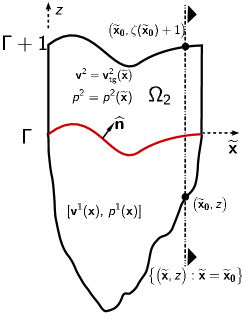
(a) Limit Solutions in the Reference Domain

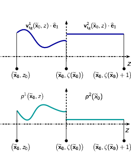
(b) Velocity and Pressure Schematic Traces for the solution on the hyperplane $\{(\widetilde{\mathbf{x}},z):\widetilde{\mathbf{x}}=\widetilde{\mathbf{x}}_{0}\}$.

Figure 2: Figure (a) depicts the dependence of the limit solution $[\mathbf{v},p]$, for both regions $\Omega_{1}$ and $\Omega_{2}$ and a generic hyperplane $\{(\widetilde{\mathbf{x}},z):\widetilde{\mathbf{x}}=\widetilde{\mathbf{x}}_{0}\}$. Figure (b) shows plausible schematics for traces of the velocity and pressure on the hyperplane $\{(\widetilde{\mathbf{x}},z):\widetilde{\mathbf{x}}=\widetilde{\mathbf{x}}_{0}\}$, depicted in Figure (a).

Theorem 8 (Convergence of Pressures)

Let $\big{[}\mathbf{v}^{\,\epsilon},p^{\,\epsilon}\big{]}\in\mathbf{X}\times\mathbf{Y}$ be the solution of problem (30). There exists a subsequence, still denoted $(p^{\,\epsilon}:\epsilon>0)$ verifying the following.

1. There exists $p^{1}\in H^{1}(\Omega_{1})$ such that

   $$p^{1,\epsilon}\rightarrow p^{1}\text{ weakly in }H^{1}(\Omega_{1})\text{ and strongly in }\,L^{2}(\Omega_{1}),$$ (44a)

   $${\mathcal{Q}}\mathbf{v}^{1}+\bm{\nabla}p^{1}=0\text{ in }\Omega_{1}, p^{1}=0\text{ on }\partial\Omega_{1}-\Gamma,$$ (44b)

   with $\mathbf{v}^{1}$ the weak limit of Statement (39a).

2. There exists $p^{2}\in L^{2}(\Omega_{2})$ such that

   $$p^{\,2,\epsilon}\rightarrow p^{2}\quad\text{weakly in }\,L^{2}(\Omega_{2}).$$ (45)

3. The pressure $p=\big{[}p^{1},p^{2}\big{]}$ belongs to $L^{2}(\Omega)$.

Proof 8

1. (The proof is identical to part (i) Lemma 12 in [14], we write it here for the sake of completeness.) Due to (26b) and (36) it follows that

   $$\big{\|}\bm{\nabla}p^{1,\epsilon}\big{\|}_{0,\Omega_{1}}=\big{\|}\sqrt{{\mathcal{Q}}}\,\mathbf{v}^{1,\epsilon}\big{\|}_{0,\Omega_{1}}\leq C,$$

   with $C>0$ an adequate positive constant. From (27a), the Poincaré inequality implies there exists a constant $\widetilde{C}>0$ satisfying

   $$\big{\|}p^{1,\epsilon}\big{\|}_{1,\Omega_{1}}\leq\widetilde{C}\,\big{\|}\bm{\nabla}p^{1,\epsilon}\big{\|}_{0,\Omega_{1}}, \text{for all }\,\epsilon>0.$$ (46)

   Therefore, the sequence $(p^{1,\epsilon}:\epsilon>0)$ is bounded in $H^{1}(\Omega_{1})$ and the convergence statement (44a) follows directly. Again, given that $p^{1,\epsilon}$ satisfies the Darcy equation (26b) and that the gradient $\bm{\nabla}$ is linear and continuous in $H^{1}(\Omega_{1})$ the equality ${\mathcal{Q}}\mathbf{v}^{1}+\bm{\nabla}p^{1}=0$ in (44b) follows. Finally, since $p^{1,\epsilon}\big{|}_{\Omega_{1}-\Gamma}=0$ for every element of the weakly convergent subsequence and the trace map $\varphi\mapsto\varphi\big{|}_{\Gamma}$ is linear, it follows that $p^{1}$ satisfies the boundary condition in (44b).

2. In order to show that the sequence $(p^{\,2,\epsilon}:\epsilon>0)$ is bounded in $L^{2}(\Omega_{2})$, take any $\phi\in C_{0}^{\infty}(\Omega_{2})$ and define the auxiliary function

   $$\varpi(\widetilde{\mathbf{x}},z)\overset{\mathbf{def}}{=}\int_{z}^{\zeta(\widetilde{\mathbf{x}})+1}\phi(\widetilde{\mathbf{x}},t)\,dt, \zeta(\widetilde{\mathbf{x}})\leq z\leq\zeta(\widetilde{\mathbf{x}})+1.$$ (47)

   Since $\zeta\in C^{2}(G)$, it is clear that $\varpi\in H^{1}(\Omega_{2})$ and $\|\varpi\|_{\,1,\Omega_{2}}\leq C\|\phi\|_{0,\Omega_{2}}$. Hence, the function $\mathbf{w}^{2}\overset{\mathbf{def}}{=}\big{(}\mathbf{0}_{T},\varpi\big{)}=\varpi\,\bm{\widehat{e}}_{N}$ belongs to $\mathbf{X}_{2}$, moreover

   $$\begin{split}\|\,\mathbf{w}^{2}\,\|_{0,\Omega_{2}}+\|\,\partial_{z}\,\mathbf{w}^{2}\,\|_{0,\Omega_{2}}&\leq\widetilde{C}\,\|\,\phi\,\|_{0,\Omega_{2}},\\ \|\mathbf{w}^{2}(\operatorname*{tg})\big{|}_{\Gamma}\|_{0,\Gamma}=\|\mathbf{w}_{\,\operatorname*{tg}}^{2}\big{|}_{\Gamma}\|_{0,\Gamma}&\leq\widetilde{C}\,\|\,\phi\,\|_{0,\Omega_{2}}.\end{split}$$ (48)

   Here, the second inequality follows from the first one and due to the estimate (32a). Next, observe that $\varpi\,\bm{\widehat{e}}_{N}\cdot\bm{\widehat{n}}(\cdot)\,\bm{\mathbbm{1}}_{\Gamma}\in L^{2}(\Gamma)\subseteq H^{-1/2}(\partial\Omega_{1})$ then, Lemma 1 gives the existence of a function $\mathbf{w}^{1}\in\mathbf{H}_{\operatorname*{div}}\,(\Omega_{1})$ such that

   $$\begin{split}\mathbf{w}^{1}\cdot\bm{\widehat{n}}=\mathbf{w}^{2}\cdot\bm{\widehat{n}}=\varpi(\widetilde{\mathbf{x}},\zeta(\widetilde{\mathbf{x}}))\bm{\widehat{e}}_{N}\cdot\bm{\widehat{n}}(\widetilde{\mathbf{x}})&=\int_{\zeta(\widetilde{\mathbf{x}})}^{\zeta(\widetilde{\mathbf{x}})+1}\phi\,(\widetilde{\mathbf{x}},t)\,dt\text{ on }\Gamma,\\ \mathbf{w}^{1}\cdot\bm{\widehat{n}}&=0\text{ on }\partial\Omega_{1}-\Gamma,\\ \|\mathbf{w}^{1}\|_{\,\mathbf{H}_{\operatorname*{div}}(\Omega_{1})}&\leq\|\varpi\,\bm{\widehat{e}}_{N}\cdot\bm{\widehat{n}}(\cdot)\|_{0,\Gamma}\leq C\|\phi\|_{0,\Omega_{2}}.\end{split}$$ (49)

   Here, the last inequality holds because $\sup\{\bm{\widehat{n}}(\widetilde{\mathbf{x}})\cdot\bm{\widehat{e}}_{N}:\widetilde{\mathbf{x}}\in\Gamma\}<\infty$. Hence, the function $\mathbf{w}\overset{\mathbf{def}}{=}[\mathbf{w}^{1},\mathbf{w}^{2}]$ belongs to the space $\mathbf{X}$. Testing (30a) with $\mathbf{w}$ yields

   $$\begin{split}\int_{\Omega_{1}}{\mathcal{Q}}\,\mathbf{v}^{1,\epsilon}\cdot\mathbf{w}^{1}&-\int_{\Omega_{1}}p^{1,\epsilon}\,\bm{\nabla\cdot}\mathbf{w}^{1}+\int_{\Omega_{2}}\,p^{\,2,\epsilon}\,\phi+\epsilon^{2}\int_{\Omega_{2}}\mu\,\bm{D}^{\epsilon}\,\mathbf{v}^{\,2,\epsilon}\bm{:}\,\bm{D}^{\epsilon}\,\mathbf{w}^{2}-\int_{\Omega_{2}}\mu\,\partial_{z}\,\mathbf{v}_{\scriptscriptstyle N}^{\,2,\epsilon}\,\phi\\ &+\alpha\int_{\,\Gamma}\big{(}\mathbf{v}^{1,\epsilon}\cdot\bm{\widehat{n}}\big{)}\big{(}\mathbf{w}^{1}\cdot\bm{\widehat{n}}\,\big{)}dS+\epsilon^{2}\int_{\,\Gamma}\gamma\,\sqrt{{\mathcal{Q}}}\,\mathbf{v}_{\,\operatorname*{tg}}^{2,\epsilon}\cdot\mathbf{w}_{\,\operatorname*{tg}}^{2}dS=\epsilon\int_{\Omega_{2}}\mathbf{f}^{2,\epsilon}_{N}\,\varpi.\end{split}$$ (50)

   Applying the Cauchy-Bunyakowsky-Schwarz inequality to the integrals and reordering we get

   $$\begin{split}\Big{|}\int_{\Omega_{2}}\,p^{\,2,\epsilon}\,\phi\Big{|}\leq\,&C_{1}\,\big{\|}\,\mathbf{v}^{1,\epsilon}\,\big{\|}_{0,\Omega_{1}}\big{\|}\,\mathbf{w}^{1}\,\big{\|}_{0,\Omega_{1}}+\big{\|}\,p^{1,\epsilon}\,\big{\|}_{0,\Omega_{1}}\big{\|}\,\bm{\nabla\cdot}\mathbf{w}^{1}\,\big{\|}_{0,\Omega_{1}}+C_{2}\,\big{\|}\,\epsilon\,\bm{D}^{\epsilon}\,\mathbf{v}^{\,2,\epsilon}\big{\|}_{0,\Omega_{2}}\big{\|}\,\epsilon\,\bm{D}^{\epsilon}\,\mathbf{w}^{2}\,\big{\|}_{0,\Omega_{2}}\\ &+C_{3}\,\big{\|}\,\partial_{z}\,\mathbf{v}_{\scriptscriptstyle N}^{\,2,\epsilon}\,\big{\|}_{0,\Omega_{2}}\big{\|}\,\phi\,\big{\|}_{0,\Omega_{2}}+C_{4}\,\big{\|}\,\mathbf{v}^{1,\epsilon}\cdot\bm{\widehat{n}}\,\big{\|}_{0,\Gamma}\big{\|}\,\mathbf{w}^{2}\cdot\bm{\widehat{n}}\,\big{\|}_{0,\Gamma}\\ &+C_{5}\,\epsilon\,\big{\|}\epsilon\,\mathbf{v}_{\,\operatorname*{tg}}^{2,\epsilon}\big{\|}_{0,\Gamma}\big{\|}\mathbf{w}_{\,\operatorname*{tg}}^{2}\big{\|}_{0,\Gamma}+\big{\|}\,\epsilon\,\mathbf{f}^{2,\epsilon}_{N}\,\big{\|}_{0,\Omega_{2}}\big{\|}\,\varpi\,\big{\|}_{0,\Omega_{2}}.\end{split}$$

   We pursue estimates in terms of $\|\phi\|_{0,\Omega_{2}}$, to that end we first apply the fact that all the terms involving the solution on the right hand side, i.e. $\mathbf{v}^{1,\epsilon},\,p^{1,\epsilon},\,\epsilon\,\bm{D}^{\epsilon}\,\mathbf{v}^{\,2,\epsilon},\,\partial_{z}\,\mathbf{v}_{\scriptscriptstyle N}^{\,2,\epsilon},\,\mathbf{v}^{1,\epsilon}\cdot\bm{\widehat{n}}$ and $\mathbf{v}_{\,\operatorname*{tg}}^{2,\epsilon}\big{|}_{\Gamma}$ are bounded; in addition, the forcing term $\epsilon\,\mathbf{f}^{2,\epsilon}_{N}$ is bounded. Replacing these by a generic constant on the right hand side we have

   $$\begin{split}\Big{|}\int_{\Omega_{2}}\,p^{\,2,\epsilon}\,\phi\Big{|}\leq&C\Big{(}\big{\|}\,\mathbf{w}^{1}\,\big{\|}_{0,\Omega_{1}}+\big{\|}\,\bm{\nabla\cdot}\mathbf{w}^{1}\,\big{\|}_{0,\Omega_{1}}\\ &+\big{\|}\,\epsilon\,\bm{D}^{\epsilon}\,\mathbf{w}^{2}\,\big{\|}_{0,\Omega_{2}}+\big{\|}\,\phi\,\big{\|}_{0,\Omega_{2}}+\big{\|}\,\mathbf{w}^{2}\cdot\bm{\widehat{n}}\,\big{\|}_{0,\Gamma}+\epsilon\,\big{\|}\mathbf{w}_{\,\operatorname*{tg}}^{2}\big{\|}_{0,\Gamma}+\big{\|}\,\varpi\,\big{\|}_{0,\Omega_{2}}\Big{)}.\end{split}$$ (51)

   In the expression above the first summand of the second line needs further analysis, we have

   $$\begin{split}\big{\|}\,\epsilon\,\bm{D}^{\epsilon}\,\mathbf{w}^{2}\,\big{\|}_{0,\Omega_{2}}&=\big{\|}\,\epsilon\,\bm{\nabla}_{\!\!\scriptscriptstyle T}\,\mathbf{w}^{2}+(\epsilon-1)\,\partial_{z}\,\mathbf{w}^{2}\,\bm{\nabla}_{\!\!\scriptscriptstyle T}^{t}\zeta\,\big{\|}_{0,\Omega_{2}}\\ &\leq\epsilon\,\big{\|}\,\bm{\nabla}_{\!\!\scriptscriptstyle T}\,\mathbf{w}^{2}+\partial_{z}\,\mathbf{w}^{2}\,\bm{\nabla}_{\!\!\scriptscriptstyle T}^{t}\zeta\,\big{\|}_{0,\Omega_{2}}+\big{\|}\,\partial_{z}\,\mathbf{w}^{2}\,\bm{\nabla}_{\!\!\scriptscriptstyle T}^{t}\zeta\,\big{\|}_{0,\Omega_{2}}\\ &\leq\epsilon\,\big{\|}\,\bm{\nabla}_{\!\!\scriptscriptstyle T}\,\mathbf{w}^{2}+\partial_{z}\,\mathbf{w}^{2}\,\bm{\nabla}_{\!\!\scriptscriptstyle T}^{t}\zeta\,\big{\|}_{0,\Omega_{2}}+\big{\|}\,\partial_{z}\,\mathbf{w}^{2}\big{\|}_{0,\Omega_{2}}\big{\|}\bm{\nabla}_{\!\!\scriptscriptstyle T}^{t}\,\zeta\,\big{\|}_{0,\Omega_{2}}.\end{split}$$

   Combining (48) with the expression above we conclude

   $$\big{\|}\,\epsilon\,\bm{D}^{\epsilon}\,\mathbf{w}^{2}\,\big{\|}_{0,\Omega_{2}}\\ \leq\epsilon\,\big{\|}\,\bm{\nabla}_{\!\!\scriptscriptstyle T}\,\mathbf{w}^{2}+\partial_{z}\,\mathbf{w}^{2}\bm{\nabla}_{\!\!\scriptscriptstyle T}^{t}\,\zeta\,\big{\|}_{0,\Omega_{2}}+C\,\big{\|}\phi\big{\|}_{0,\Omega_{2}}.$$ (52)

   Back to the equation (51), the two summands on the left hand side of the first line are bounded by a multiple of $\|\,\phi\,\|_{0,\Omega_{2}}$ due to (48). The first two summands on the third line are trace terms which are also controlled by a multiple of $\|\,\phi\,\|_{0,\Omega_{2}}$ due to (48). The third summand on the third line is trivially controlled by $\|\,\phi\,\|_{0,\Omega_{2}}$ due to its construction. Combining all these observations with (52) we get

   $$\Big{|}\int_{\Omega_{2}}\,p^{\,2,\epsilon}\,\phi\Big{|}\\ \leq\epsilon\,\big{\|}\,\bm{\nabla}_{\!\!\scriptscriptstyle T}\,\mathbf{w}^{2}+\partial_{z}\,\mathbf{w}^{2}\,\bm{\nabla}_{\!\!\scriptscriptstyle T}^{t}\zeta\,\big{\|}_{0,\Omega_{2}}+C\;\big{\|}\,\phi\,\big{\|}_{0,\Omega_{2}},$$

   where $C>0$ is a new generic constant. The last inequality holds since all the summands in the parenthesis are bounded due to the estimates (35), (46) and the Hypothesis 3. Taking upper limit when $\epsilon\rightarrow 0$, in the previous expression we get

   $$\limsup_{\,\epsilon\,\downarrow\,0}\Big{|}\int_{\Omega_{2}}\,p^{\,2,\epsilon}\,\phi\Big{|}\leq C\,\big{\|}\phi\big{\|}_{0,\Omega_{2}}.$$ (53)

   The above holds for any $\phi\in C_{0}^{\infty}(\Omega_{2})$, then the sequence $(p^{\,2,\epsilon}:\epsilon>0\,)\subset L^{2}(\Omega_{2})$ is bounded and consequently the convergence statement (45) follows.

3. From the previous part it is clear that the sequence $\big{(}[p^{1,\epsilon},p^{\,2,\epsilon}]:\epsilon>0\big{)}$ is bounded in $L^{2}(\Omega)$, therefore $p$ also belongs to $L^{2}\Omega)$ and the proof is complete.

Remark 9

Notice that the upwards normal vector $\bm{\widehat{n}}$ orthogonal to the surface $\Gamma$ is given by the expression

$$\bm{\widehat{n}}=\frac{1}{|(-\bm{\nabla}_{\!\!\scriptscriptstyle T}\zeta,1)|}\begin{Bmatrix}-\bm{\nabla}_{\!\!\scriptscriptstyle T}^{t}\zeta\\ 1\end{Bmatrix}$$ (54a)

and the normal derivative satisfies

$$|(-\bm{\nabla}_{\!\!\scriptscriptstyle T}\zeta,1)|\partial_{\,\bm{\widehat{n}}}=|(-\bm{\nabla}_{\!\!\scriptscriptstyle T}\zeta,1)|\frac{\partial}{\partial\bm{\widehat{n}}}=\bm{\widehat{n}}\cdot\bm{\nabla},\quad\text{ on }\Gamma.$$ (54b)

We use the identities above to identify the dependence of $\bm{\chi}$, $\xi$ and $p^{2}$, see Figure 2.

Theorem 9

Let $\bm{\chi}$, $\xi$ be the higher order limiting terms in Corollary 7 (ii) and (iii). Let $p^{2}$ be the limit pressure in $\Omega_{2}$ in Lemma 8 (ii). Then

$$\partial_{z}\,\xi=-\mathbf{v}^{1}\cdot\bm{\widehat{n}}\big{|}_{\Gamma}, \xi(\widetilde{\mathbf{x}},z)=\mathbf{v}^{1}\cdot\bm{\widehat{n}}(\widetilde{\mathbf{x}})\big{(}1-z\big{)},\quad\text{ for }\zeta(\widetilde{\mathbf{x}})\leq z\leq\zeta(\widetilde{\mathbf{x}})+1.$$ (55a)

$$p^{2}=p^{2}(\widetilde{\mathbf{x}}).$$ (55b)

$$\bm{\chi}=\bm{\chi}(\widetilde{\mathbf{x}}), \bm{\chi}\cdot\bm{\widehat{n}}=-\mathbf{v}^{1}\cdot\bm{\widehat{n}}\quad\text{ on }\Gamma.$$ (55c)

In particular, notice that $\partial_{z}\xi=\partial_{z}\xi(\widetilde{\mathbf{x}})$.

Proof 9

Take $\Phi=\left(0,\,\varphi^{2}\right)\in\mathbf{Y}$, test (30b) and reordering the summands conveniently, we have

$$\begin{split}0&=\epsilon\int_{\Omega_{2}}\bm{\nabla}_{\!\!\scriptscriptstyle T}\bm{\cdot}\mathbf{v}_{\scriptscriptstyle T}^{\,2,\epsilon}\,\varphi^{2}+\epsilon\int_{\Omega_{2}}\partial_{z}\mathbf{v}_{\scriptscriptstyle T}^{\,2,\epsilon}\cdot\bm{\nabla}_{\!\!\scriptscriptstyle T}\zeta\,\varphi^{2}-\int_{\Omega_{2}}\partial_{z}\mathbf{v}_{\scriptscriptstyle T}^{\,2,\epsilon}\cdot\bm{\nabla}_{\!\!\scriptscriptstyle T}\zeta\,\varphi^{2}+\int_{\Omega_{2}}\partial_{z}\mathbf{v}_{\scriptscriptstyle N}^{\,2,\epsilon}\,\varphi^{2}\\ &=\int_{\Omega_{2}}\bm{\nabla}_{\!\!\scriptscriptstyle T}\bm{\cdot}\left(\epsilon\,\mathbf{v}_{\scriptscriptstyle T}^{\,2,\epsilon}\right)\varphi^{2}+\int_{\Omega_{2}}\partial_{z}\big{(}\epsilon\,\mathbf{v}_{\scriptscriptstyle T}^{\,2,\epsilon}\big{)}\cdot\bm{\nabla}_{\!\!\scriptscriptstyle T}\zeta\,\varphi^{2}+\int_{\Omega_{2}}\big{(}\partial_{z}\,\mathbf{v}_{\scriptscriptstyle T}^{\,2,\epsilon},\,\partial_{z}\,\mathbf{v}_{\scriptscriptstyle N}^{\,2,\epsilon}\big{)}\cdot\big{(}-\bm{\nabla}_{\!\!\scriptscriptstyle T}\zeta,\,1\big{)}\,\varphi^{2}\\ &=\int_{\Omega_{2}}\bm{\nabla}_{\!\!\scriptscriptstyle T}\bm{\cdot}\left(\epsilon\,\mathbf{v}_{\scriptscriptstyle T}^{\,2,\epsilon}\right)\varphi^{2}+\int_{\Omega_{2}}\partial_{z}\left(\epsilon\,\mathbf{v}_{\scriptscriptstyle T}^{\,2,\epsilon}\right)\cdot\bm{\nabla}_{\!\!\scriptscriptstyle T}\zeta\,\varphi^{2}+\int_{\Omega_{2}}\big{|}\big{(}-\bm{\nabla}_{\!\!\scriptscriptstyle T}\zeta,\,1\big{)}\big{|}\,\partial_{z}\left(\mathbf{v}^{\,2,\epsilon}\cdot\bm{\widehat{n}}\right)\varphi^{2}.\end{split}$$

Letting $\epsilon\,\downarrow\,0$ in the expression above we get

$$\int_{\Omega_{2}}\bm{\nabla}_{\!\!\scriptscriptstyle T}\bm{\cdot}\mathbf{v}^{2}\varphi^{2}\ +\int_{\Omega_{2}}\partial_{z}\mathbf{v}^{2}\cdot\bm{\nabla}_{\!\!\scriptscriptstyle T}\zeta\,\varphi^{2}+\int_{\Omega_{2}}\big{|}\big{(}-\bm{\nabla}_{\!\!\scriptscriptstyle T}\zeta,\,1\big{)}\big{|}\,\partial_{z}\,\xi\,\varphi^{2}=0.$$

Recalling Equation (40c) we have $\partial_{z}\,\mathbf{v}^{2}=0$; thus

$$\int_{\Omega_{2}}\bm{\nabla}_{\!\!\scriptscriptstyle T}\bm{\cdot}\mathbf{v}^{2}\,\varphi^{2}+\int_{\Omega_{2}}\big{|}\big{(}-\bm{\nabla}_{\!\!\scriptscriptstyle T}\zeta,\,1\big{)}\big{|}\partial_{z}\,\xi\,\varphi^{2}=0.$$

Since the above holds for all $\varphi^{2}\in L_{\,0}^{2}(\Omega_{2})$ it follows that

$$\bm{\nabla}_{\!\!\scriptscriptstyle T}\bm{\cdot}\mathbf{v}^{2}+|(-\bm{\nabla}_{\!\!\scriptscriptstyle T}\zeta,\,1)|\partial_{z}\,\xi=c,$$

where $c$ is a constant. In the expression above we observe that two out of three terms are independent from $z$, then it follows that the third summand is also independent from $z$. Since the vector $(-\bm{\nabla}_{\!\!\scriptscriptstyle T}\zeta,\,1)$ is independent from $z$ we conclude that $\partial_{z}\xi=\partial_{z}\xi(\widetilde{\mathbf{x}})$ this, together with the boundary conditions (41b) yield the second equality in (55a).

Take $\Psi=\big{(}\phi^{\,1},\ldots,\,\phi^{\,N}\big{)}\in\left(C_{\mathbf{0}}^{\infty}(\Omega_{2})\right)^{N}$ and for $i=1,2,\ldots,N$, build the “antiderivative” $\varpi^{i}$ of $\phi^{i}$ using the rule (47) and define $\mathbf{w}^{2}=\big{(}\varpi^{1},\ldots,\,\varpi^{\,N}\big{)}$. Use Lemma 1 to construct $\mathbf{w}^{1}\in\mathbf{H}_{\operatorname*{div}}(\Omega_{1})$ such that $\mathbf{w}^{1}\cdot\bm{\widehat{n}}=\mathbf{w}^{2}\cdot\bm{\widehat{n}}$ on $\Gamma$, $\mathbf{w}^{1}\cdot\bm{\widehat{n}}=0$ on $\partial\Omega_{1}-\Gamma$ and

$$\big{\|}\mathbf{w}^{1}\big{\|}_{\,\mathbf{H}_{\operatorname*{div}}(\Omega_{1})}\leq C\big{\|}\Psi\big{\|}_{\,\mathbf{L}^{2}(\Omega_{2})}.$$ (56)

Therefore $\mathbf{w}\overset{\mathbf{def}}{=}\big{(}\mathbf{w}^{1},\,\mathbf{w}^{2}\big{)}\in\mathbf{X}_{2}$; test (30a) with $\mathbf{w}$ and regroup terms of higher order, we have

$$\begin{split}\int_{\Omega_{1}}{\mathcal{Q}}\,\mathbf{v}^{1,\epsilon}\cdot\mathbf{w}^{1}&-\int_{\Omega_{1}}p^{1,\epsilon}\,\bm{\nabla\cdot}\mathbf{w}^{1}\\ &-\epsilon\int_{\Omega_{2}}p^{\,2,\epsilon}\,\bm{\nabla}_{\!\!\scriptscriptstyle T}\bm{\cdot}\mathbf{w}_{\scriptscriptstyle T}^{2}-\epsilon\int_{\Omega_{2}}p^{\,2,\epsilon}\,\partial_{z}\,\mathbf{w}_{\scriptscriptstyle T}^{2}\cdot\bm{\nabla}_{\!\!\scriptscriptstyle T}\zeta+\int_{\Omega_{2}}p^{\,2,\epsilon}\,\partial_{z}\,\mathbf{w}_{\scriptscriptstyle T}^{2}\cdot\bm{\nabla}_{\!\!\scriptscriptstyle T}\zeta-\int_{\Omega_{2}}p^{\,2,\epsilon}\,\partial_{z}\mathbf{w}_{\scriptscriptstyle N}^{2}\\ &+\epsilon^{2}\int_{\Omega_{2}}\mu\,\bm{D}^{\epsilon}\mathbf{v}^{\,2,\epsilon}\bm{:}\bm{D}^{\epsilon}\mathbf{w}^{2}+\int_{\Omega_{2}}\mu\,\partial_{z}\,\mathbf{v}^{\,2,\epsilon}\cdot\partial_{z}\,\mathbf{w}^{2}\\ &+\alpha\int_{\,\Gamma}\big{(}\,\mathbf{v}^{1,\epsilon}\cdot\bm{\widehat{n}}\,\big{)}\,\big{(}\,\mathbf{w}^{1}\,\cdot\bm{\widehat{n}}\,\big{)}\,dS+\,\epsilon^{\,2}\int_{\Gamma}\gamma\sqrt{{\mathcal{Q}}}\,\mathbf{v}_{\,\operatorname*{tg}}^{2,\epsilon}\cdot\mathbf{w}_{\,\operatorname*{tg}}^{2}\,dS=\epsilon\,\int_{\Omega_{2}}{\mathbf{f}^{2,\epsilon}}\cdot\mathbf{w}^{2}.\end{split}$$ (57)

The limit of all the terms in the expression above when $\epsilon\,\downarrow\,0$ is clear except for one term, which we discuss independently, i.e.

$$\begin{split}\epsilon^{2}\int_{\Omega_{2}}\mu\,\bm{D}^{\epsilon}\mathbf{v}^{\,2,\epsilon}\bm{:}\bm{D}^{\epsilon}\mathbf{w}^{2}&=\epsilon^{2}\int_{\Omega_{2}}\mu\,\bm{D}^{\epsilon}\mathbf{v}^{\,2,\epsilon}\bm{:}\Big{(}\bm{\nabla}_{\!\!\scriptscriptstyle T}\,\mathbf{w}^{2}+\partial_{z}\,\mathbf{w}^{2}\bm{\nabla}_{\!\!\scriptscriptstyle T}^{t}\zeta-\frac{1}{\epsilon}\,\partial_{z}\,\mathbf{w}^{2}\bm{\nabla}_{\!\!\scriptscriptstyle T}^{t}\zeta\Big{)}\\ &=\epsilon^{2}\int_{\Omega_{2}}\mu\,\bm{D}^{\epsilon}\mathbf{v}^{\,2,\epsilon}\bm{:}\big{(}\bm{\nabla}_{\!\!\scriptscriptstyle T}\,\mathbf{w}^{2}+\partial_{z}\,\mathbf{w}^{2}\bm{\nabla}_{\!\!\scriptscriptstyle T}^{t}\zeta\big{)}+\epsilon\int_{\Omega_{2}}\mu\,\bm{D}^{\epsilon}\mathbf{v}^{\,2,\epsilon}\bm{:}\,\partial_{z}\,\mathbf{w}^{2}\big{(}-\bm{\nabla}_{\!\!\scriptscriptstyle T}^{t}\,\zeta\big{)}.\end{split}$$

In the expression above, the first summand clearly tends to zero when $\epsilon\downarrow 0$. Therefore, we focus on the second summand

$$\begin{split}\epsilon\int_{\Omega_{2}}\mu\,\bm{D}^{\epsilon}\mathbf{v}^{\,2,\epsilon}\bm{:}\,\partial_{z}\,\mathbf{w}^{2}\big{(}-\bm{\nabla}_{\!\!\scriptscriptstyle T}^{t}\,\zeta\big{)}=&\int_{\Omega_{2}}\mu\,\big{(}\bm{\nabla}_{\!\!\scriptscriptstyle T}\,\big{(}\epsilon\,\mathbf{v}^{\,2,\epsilon}\big{)}+\partial_{z}\big{(}\epsilon\,\mathbf{v}^{\,2,\epsilon}\big{)}\bm{\nabla}_{\!\!\scriptscriptstyle T}^{t}\zeta\big{)}\bm{:}\,\partial_{z}\,\mathbf{w}^{2}\big{(}-\bm{\nabla}_{\!\!\scriptscriptstyle T}^{t}\zeta\big{)}\\ &+\int_{\Omega_{2}}\mu\,\partial_{z}\mathbf{v}^{\,2,\epsilon}\big{(}-\bm{\nabla}_{\!\!\scriptscriptstyle T}^{t}\zeta\big{)}\bm{:}\,\partial_{z}\,\mathbf{w}^{2}\big{(}-\bm{\nabla}_{\!\!\scriptscriptstyle T}^{t}\zeta\big{)}.\end{split}$$

All the terms in the left hand side can pass to the limit. Recalling the statement (40a), we conclude

$$\epsilon^{2}\int_{\Omega_{2}}\mu\,\bm{D}^{\epsilon}\mathbf{v}^{\,2,\epsilon}\bm{:}\bm{D}^{\epsilon}\mathbf{w}^{2}\rightarrow\int_{\Omega_{2}}\mu\,\bm{\nabla}_{\!\!\scriptscriptstyle T}\,\mathbf{v}^{2}\bm{:}\,\partial_{z}\,\mathbf{w}^{2}\big{(}-\bm{\nabla}_{\!\!\scriptscriptstyle T}^{t}\zeta\big{)}+\int_{\Omega_{2}}\mu\,\bm{\chi}\big{(}-\bm{\nabla}_{\!\!\scriptscriptstyle T}^{t}\,\zeta\big{)}\bm{:}\partial_{z}\,\mathbf{w}^{2}\big{(}-\bm{\nabla}_{\!\!\scriptscriptstyle T}^{t}\zeta\big{)}.$$

Letting $\epsilon\downarrow 0$ in (57) and considering the equality above we get

$$\begin{split}\int_{\Omega_{1}}{\mathcal{Q}}\,\mathbf{v}^{1}\cdot\mathbf{w}^{1}-&\int_{\Omega_{1}}p^{1}\,\bm{\nabla}\cdot\mathbf{w}^{1}+\int_{\Omega_{2}}p^{2}\,\big{(}\partial_{z}\,\mathbf{w}_{\scriptscriptstyle T}^{2},\,\partial_{z}\,\mathbf{w}_{\scriptscriptstyle N}^{2}\big{)}\cdot\big{(}\bm{\nabla}_{\!\!\scriptscriptstyle T}\zeta,\,-1\big{)}+\int_{\Omega_{2}}\mu\,\bm{\nabla}_{\!\!\scriptscriptstyle T}\,\mathbf{v}^{2}\bm{:}\,\partial_{z}\,\mathbf{w}^{2}\big{(}-\bm{\nabla}_{\!\!\scriptscriptstyle T}^{t}\zeta\big{)}\\ &+\int_{\Omega_{2}}\mu\,\bm{\chi}\big{(}-\bm{\nabla}_{\!\!\scriptscriptstyle T}^{t}\zeta\big{)}\bm{:}\partial_{z}\,\mathbf{w}^{2}\big{(}-\bm{\nabla}_{\!\!\scriptscriptstyle T}^{t}\zeta\big{)}+\int_{\Omega_{2}}\mu\,\bm{\chi}\cdot\partial_{z}\,\mathbf{w}^{2}+\alpha\int_{\,\Gamma}\big{(}\mathbf{v}^{1}\cdot\bm{\widehat{n}}\,\big{)}\,\big{(}\mathbf{w}^{1}\,\cdot\bm{\widehat{n}}\big{)}\,dS=0.\end{split}$$ (58)

We develop a simpler expression for the sum of the fourth, fifth and sixth terms

$$\begin{split}\int_{\Omega_{2}}\mu\,\bm{\nabla}_{\!\!\scriptscriptstyle T}\,\mathbf{v}^{2}\bm{:}\,\partial_{z}\,\mathbf{w}^{2}&\big{(}-\bm{\nabla}_{\!\!\scriptscriptstyle T}^{t}\,\zeta\big{)}+\int_{\Omega_{2}}\mu\,\bm{\chi}\big{(}-\bm{\nabla}_{\!\!\scriptscriptstyle T}^{t}\,\zeta\big{)}\bm{:}\partial_{z}\,\mathbf{w}^{2}\big{(}-\bm{\nabla}_{\!\!\scriptscriptstyle T}^{t}\zeta\big{)}+\int_{\Omega_{2}}\mu\,\bm{\chi}\cdot\partial_{z}\,\mathbf{w}^{2}\\ &=\int_{\Omega_{2}}\mu\,\big{(}\bm{\nabla}\mathbf{v}^{2}\cdot(-\bm{\nabla}_{\!\!\scriptscriptstyle T}\zeta,\,1)\big{)}\cdot\partial_{z}\,\mathbf{w}^{2}+\int_{\Omega_{2}}\mu\,\bm{\chi}\,(-\bm{\nabla}_{\!\!\scriptscriptstyle T}\zeta,\,1)^{t}\bm{:}\,\partial_{z}\,\mathbf{w}^{2}(-\bm{\nabla}_{\!\!\scriptscriptstyle T}\,\zeta,\,1)^{t}\\ &=\int_{\Omega_{2}}\mu|(-\bm{\nabla}_{\!\!\scriptscriptstyle T}\zeta,\,1)|\,\partial_{\,\bm{\widehat{n}}}\,\mathbf{v}^{2}\cdot\partial_{z}\,\mathbf{w}^{2}+\int_{\Omega_{2}}\mu\,\bm{\chi}\cdot\partial_{z}\mathbf{w}^{2}\,(-\bm{\nabla}_{\!\!\scriptscriptstyle T}\zeta,\,1)\cdot(-\bm{\nabla}_{\!\!\scriptscriptstyle T}\zeta,\,1).\end{split}$$

Here $\partial_{\,\bm{\widehat{n}}}$ is the normal derivative defined in the identity (54b). We introduce the equality above in (58), this yields

$$\int_{\Omega_{1}}{\mathcal{Q}}\,\mathbf{v}^{1}\cdot\mathbf{w}^{1}-\int_{\Omega_{1}}p^{1}\,\bm{\nabla}\cdot\mathbf{w}^{1}-\int_{\Omega_{2}}|(-\bm{\nabla}_{\!\!\scriptscriptstyle T}\zeta,\,1)|p^{2}\,\partial_{z}\big{(}\mathbf{w}^{2}\cdot\bm{\widehat{n}}\big{)}+\int_{\Omega_{2}}\mu\,|(-\bm{\nabla}_{\!\!\scriptscriptstyle T}\zeta,\,1)|\partial_{\,\bm{\widehat{n}}}\mathbf{v}^{2}\cdot\partial_{z}\,\mathbf{w}^{2}\\ +\int_{\Omega_{2}}\mu\,\bm{\chi}\cdot\partial_{z}\,\mathbf{w}^{2}\big{|}\big{(}-\bm{\nabla}_{\!\!\scriptscriptstyle T}\zeta,\,1\big{)}\big{|}^{2}+\alpha\int_{\Gamma}\big{(}\mathbf{v}^{1}\cdot\bm{\widehat{n}}\big{)}\,\big{(}\mathbf{w}^{1}\,\cdot\bm{\widehat{n}}\big{)}\,dS=0.$$ (59)

Next, we integrate by parts the second summand in the first line, add it to the first summand and recall that $\partial_{z}\mathbf{w}^{2}=-\Psi$ by construction, thus

$$-\int_{\Gamma}p^{1}\,\big{(}\mathbf{w}^{1}\cdot\bm{\widehat{n}}\big{)}\,dS+\int_{\Omega_{2}}|(-\bm{\nabla}_{\!\!\scriptscriptstyle T}\zeta,\,1)|p^{2}\;\bm{\widehat{n}}\cdot\Psi\\ -\int_{\Omega_{2}}\mu|(-\bm{\nabla}_{\!\!\scriptscriptstyle T}\zeta,\,1)|\partial_{\,\bm{\widehat{n}}}\mathbf{v}^{2}\cdot\Psi-\int_{\Omega_{2}}\mu\,\bm{\chi}\cdot\Psi\,|(-\bm{\nabla}_{\!\!\scriptscriptstyle T}\zeta,\,1)|^{2}+\alpha\int_{\Gamma}\big{(}\mathbf{v}^{1}\cdot\bm{\widehat{n}}\big{)}\,\big{(}\mathbf{w}^{1}\,\cdot\bm{\widehat{n}}\big{)}\,dS=0.$$ (60)

In the expression above we develop the surface integrals as integrals over the projection $G$ of $\Gamma$ on $\bm{\mathbbm{R}}^{N-1}$, we get

$$-\int_{\Gamma}p^{1}\,\big{(}\mathbf{w}^{1}\cdot\bm{\widehat{n}}\big{)}\,dS+\alpha\int_{\Gamma}\big{(}\mathbf{v}^{1}\cdot\bm{\widehat{n}}\big{)}\,\big{(}\mathbf{w}^{1}\cdot\bm{\widehat{n}}\big{)}\,dS\\ =\int_{G}\frac{1}{\bm{\widehat{n}}\cdot\bm{\widehat{e}}_{N}}\,\big{[}-p^{1}\big{|}_{\Gamma}+\alpha\,\big{(}\mathbf{v}^{1}\cdot\bm{\widehat{n}}\,\big{|}_{\Gamma}\big{)}\big{]}\big{(}\mathbf{w}^{1}\cdot\bm{\widehat{n}}\,\big{|}_{\Gamma}\big{)}\,d\widetilde{\mathbf{x}}.$$

Recalling that $\displaystyle\mathbf{w}^{1}\cdot\bm{\widehat{n}}=\int_{\zeta(\widetilde{\mathbf{x}})}^{\zeta(\widetilde{\mathbf{x}})+1}\Psi(\widetilde{\mathbf{x}},z)\,dz\cdot\bm{\widehat{n}}$ on $\Gamma$, the equality above transforms in

$$\begin{split}\int_{G}\frac{1}{\bm{\widehat{n}}\cdot\bm{\widehat{e}}_{N}}\,\big{[}-p^{1}\big{|}_{\Gamma}+\alpha\,\big{(}\mathbf{v}^{1}\cdot\bm{\widehat{n}}\,\big{|}_{\Gamma}\big{)}\big{]}\,&\int_{\,\zeta(\widetilde{\mathbf{x}})}^{\zeta(\widetilde{\mathbf{x}})+1}\Psi(\widetilde{\mathbf{x}},z)\,dz\cdot\bm{\widehat{n}}(\widetilde{\mathbf{x}})\,d\widetilde{\mathbf{x}}\\ &=\int_{G}\int_{\,\zeta(\widetilde{\mathbf{x}})}^{\zeta(\widetilde{\mathbf{x}})+1}\frac{1}{\bm{\widehat{n}}\cdot\bm{\widehat{e}}_{N}}\,\big{[}-p^{1}\big{|}_{\Gamma}+\alpha\,\big{(}\mathbf{v}^{1}\cdot\bm{\widehat{n}}\,\big{|}_{\Gamma}\big{)}\big{]}(\widetilde{\mathbf{x}})\,\bm{\widehat{n}}(\widetilde{\mathbf{x}})\cdot\Psi(\widetilde{\mathbf{x}},z)\,dz\,d\widetilde{\mathbf{x}}\\ &=\int_{\Omega_{2}}\frac{1}{\bm{\widehat{n}}\cdot\bm{\widehat{e}}_{N}}\,\big{[}-p^{1}\big{|}_{\Gamma}+\alpha\,\big{(}\mathbf{v}^{1}\cdot\bm{\widehat{n}}\,\big{|}_{\Gamma}\big{)}\big{]}\,\bm{\widehat{n}}\cdot\Psi\,dz\,d\widetilde{\mathbf{x}}.\end{split}$$

Introducing the latter in (60) we have

$$\int_{\Omega_{2}}\frac{1}{\bm{\widehat{n}}\cdot\bm{\widehat{e}}_{N}}\,\big{[}-p^{1}\big{|}_{\Gamma}+\alpha\,\big{(}\mathbf{v}^{1}\cdot\bm{\widehat{n}}\,\big{|}_{\Gamma}\big{)}\big{]}\bm{\widehat{n}}\cdot\Psi\,dz\,d\widetilde{\mathbf{x}}+\int_{\Omega_{2}}|(-\bm{\nabla}_{\!\!\scriptscriptstyle T}\zeta,\,1)|p^{2}\,\bm{\widehat{n}}\cdot\Psi\,d\widetilde{\mathbf{x}}\,dz\\ -\int_{\Omega_{2}}\mu\,|(-\bm{\nabla}_{\!\!\scriptscriptstyle T}\zeta,\,1)|\partial_{\,\bm{\widehat{n}}}\mathbf{v}^{2}\cdot\Psi\,d\widetilde{\mathbf{x}}\,dz-\int_{\Omega_{2}}\mu\,\big{|}\big{(}-\bm{\nabla}_{\!\!\scriptscriptstyle T}\zeta,\,1\big{)}\big{|}^{2}\,\bm{\chi}\cdot\Psi\,d\widetilde{\mathbf{x}}\,dz=0.$$

Since the above holds for all $\Psi\in\big{(}C_{0}^{\infty}(\Omega_{2})\big{)}^{N}$, we conclude

$$\frac{1}{\bm{\widehat{n}}\cdot\bm{\widehat{e}}_{N}}\,\big{[}-p^{1}\big{|}_{\Gamma}+\alpha\,\big{(}\mathbf{v}^{1}\cdot\bm{\widehat{n}}\,\big{|}_{\Gamma}\big{)}\big{]}\bm{\widehat{n}}+|(-\bm{\nabla}_{\!\!\scriptscriptstyle T}\zeta,\,1)|p^{2}\,\bm{\widehat{n}}\\ -\mu\,|(-\bm{\nabla}_{\!\!\scriptscriptstyle T}\zeta,\,1)|\partial_{\,\bm{\widehat{n}}}\mathbf{v}^{2}-\mu\,|(-\bm{\nabla}_{\!\!\scriptscriptstyle T}\zeta,\,1)|^{2}\,\bm{\chi}=0\,,\quad\text{in}\;\mathbf{L}^{2}(\Omega_{2}).$$ (61)

In order to get the normal balance on the interface we could repeat the previous strategy but using $\Psi\in C_{\,0}^{\,\infty}(\Omega_{2})^{N}$ such that $\Psi=\big{(}\Psi\cdot\bm{\widehat{n}}\big{)}\,\bm{\widehat{n}}$, i.e. such that it is arallel to the normal direction. This would be equivalent to replace $\Psi$ by $\big{(}\Psi\cdot\bm{\widehat{n}}\big{)}\,\bm{\widehat{n}}$ in all the previous equations. Consequently, in order to get the normal balance, it suffices to apply $\big{(}\cdot\dfrac{\bm{\widehat{n}}}{|(-\bm{\nabla}_{\!\!\scriptscriptstyle T}\zeta,\,1)|^{2}}\big{)}$ to Equation (61); such operation yields:

$$\frac{1}{\bm{\widehat{n}}\cdot\bm{\widehat{e}}_{N}}\,\frac{1}{|(-\bm{\nabla}_{\!\!\scriptscriptstyle T}\zeta,\,1)|^{2}}\,\big{[}-p^{1}\big{|}_{\Gamma}+\alpha\,\big{(}\mathbf{v}^{1}\cdot\bm{\widehat{n}}\,\big{|}_{\Gamma}\big{)}\big{]}\\ +\,\frac{1}{|(-\bm{\nabla}_{\!\!\scriptscriptstyle T}\zeta,\,1)|}\,p^{2}\,-\mu\,\frac{1}{|(-\bm{\nabla}_{\!\!\scriptscriptstyle T}\zeta,\,1)|}\,\partial_{\,\bm{\widehat{n}}}\mathbf{v}^{2}\cdot\bm{\widehat{n}}-\mu\,\partial_{z}\,\xi=0.$$ (62)

In the expression above the identity (42) has been used. Also notice that all the terms are independent from $z$, then the equation (55b) follows. Consequently, all the terms but the last in (61) are independent of $z$, therefore we conclude $\bm{\chi}$ is independent from $z$. Recalling (42) and (55a) the second equality in (55c) follows and the proof is complete.

4 The Limiting Problem

In this section we derive the form of the limiting problem and characterize it as a Darcy-Brinkman coupled system, where the Brinkman equation takes place in a $N-1$-dimensional manifold of $\bm{\mathbbm{R}}^{N}$. First, we need to introduce some extra hypotheses to complete the analysis.

Hypothesis 4

In the following, it will be assumed that the sequence of forcing terms $\big{(}\mathbf{f}^{2,\epsilon}:\epsilon>0\big{)}\subseteq\mathbf{L}^{2}(\Omega_{2})$ and $\big{(}h^{1,\epsilon}:\epsilon>0\big{)}\subseteq L^{2}(\Omega_{1})$ are weakly convergent i.e., there exist $\mathbf{f}^{2}\in\mathbf{L}^{2}(\Omega_{2})$ and $h^{1}\in L^{2}(\Omega_{1})$ such that

$$\mathbf{f}^{2,\epsilon}\rightharpoonup\mathbf{f}^{2}, h^{1,\epsilon}\rightharpoonup h^{1}\,.$$ (63)

4.1 The Tangential Behavior of the Limiting Problem

Recalling (40c) and (42) clearly the lower order limiting velocity has the structure

$$\begin{Bmatrix}\mathbf{v}_{\operatorname*{tg}}^{\,2}\\ 0\end{Bmatrix}=\begin{Bmatrix}\mathbf{v}_{\operatorname*{tg}}^{\,2}(\widetilde{\mathbf{x}})\\ 0\end{Bmatrix}.$$ (64)

The above motivates the following definition.

Definition 5

Let $\widetilde{\mathbf{x}}\mapsto U(\widetilde{\mathbf{x}})$ be the matrix map introduced in Definition 2. Define the space $\mathbf{X}_{\operatorname*{tg}}\subseteq\mathbf{X}_{2}$ by

$$\mathbf{X}_{\operatorname*{tg}}\overset{\mathbf{def}}{=}\bigg{\{}\mathbf{w}^{2}\in\mathbf{X}_{2}:\mathbf{w}^{2}=U(\widetilde{\mathbf{x}})\begin{Bmatrix}\mathbf{w}_{\,\operatorname*{tg}}^{2}(\widetilde{\mathbf{x}})\\ 0\end{Bmatrix}\bigg{\}},$$ (65)

endowed with the $H^{1}(\Omega_{2})$-norm.

We have the following result

Lemma 10

The space $\mathbf{X}_{\operatorname*{tg}}\subset\mathbf{X}_{2}$ is closed.

Proof 10

Let $\big{(}\mathbf{w}^{2}\left(\ell\right):\ell\in\bm{\mathbbm{N}}\big{)}\subset\mathbf{X}_{\operatorname*{tg}}$ and $\mathbf{w}^{2}\in\mathbf{X}_{2}$ be such that $\big{\|}\mathbf{w}^{2}\big{(}\ell\big{)}-\mathbf{w}^{2}\big{\|}_{1,\Omega_{2}}\,\rightarrow 0$. We must show that $\mathbf{w}^{2}\in\mathbf{X}_{\operatorname*{tg}}$. First notice that the convergence in $\mathbf{X}_{2}$ implies $\big{\|}\mathbf{w}^{2}\big{(}\ell\big{)}-\mathbf{w}^{2}\big{\|}_{0,\Omega_{2}}\,\rightarrow 0$. Recalling (20) and the fact that $U(\widetilde{\mathbf{x}})$ is orthogonal, we have

$$\begin{bmatrix}U^{T,\operatorname*{tg}}&U^{T,\bm{\widehat{n}}}\\ U^{N,\operatorname*{tg}}&U^{N,\bm{\widehat{n}}}\end{bmatrix}^{t}(\widetilde{\mathbf{x}})\begin{Bmatrix}\mathbf{w}_{\scriptscriptstyle T}^{2}\left(\ell\right)\\[3.0pt] \mathbf{w}_{\scriptscriptstyle N}^{2}\left(\ell\right)\end{Bmatrix}(\widetilde{\mathbf{x}})=\begin{Bmatrix}\mathbf{w}_{\,\operatorname*{tg}}^{2}\left(\ell\right)\\[3.0pt] 0\end{Bmatrix}(\widetilde{\mathbf{x}}).$$

In the identity above, we notice that $\mathbf{w}_{\scriptscriptstyle T}^{2}\big{(}\ell\big{)},\mathbf{w}_{\scriptscriptstyle T}^{2}\big{(}\ell\big{)}$ are convergent in the $H^{1}$-norm and the orthonormal matrix $U$, has differentiability and boundedness properties. Therefore, we conclude that $\mathbf{w}_{\,\operatorname*{tg}}^{2}\big{(}\ell\big{)}$ is convergent in the $H_{1}$-norm, we denote the limit by $\mathbf{w}_{\,\operatorname*{tg}}^{2}=\mathbf{w}_{\,\operatorname*{tg}}^{2}\big{(}\widetilde{\mathbf{x}},z\big{)}$. Now take the limit in the expression above in the $L^{2}$-sense; there are no derivatives involved, then we have

$$\begin{bmatrix}U^{T,\operatorname*{tg}}&U^{T,\bm{\widehat{n}}}\\ U^{N,\operatorname*{tg}}&U^{N,\bm{\widehat{n}}}\end{bmatrix}^{t}(\widetilde{\mathbf{x}})\begin{Bmatrix}\mathbf{w}_{\scriptscriptstyle T}^{2}\\[3.0pt] \mathbf{w}_{\scriptscriptstyle N}^{2}\end{Bmatrix}(\widetilde{\mathbf{x}})=\begin{Bmatrix}\mathbf{w}_{\,\operatorname*{tg}}^{2}\big{(}\widetilde{\mathbf{x}},z\big{)}\\[3.0pt] 0\end{Bmatrix}.$$

Observe that the latter expression implicitly states that $\mathbf{w}_{\,\operatorname*{tg}}^{2}=\mathbf{w}_{\,\operatorname*{tg}}^{2}(\widetilde{\mathbf{x}})$. Finally, applying the inverse matrix again we have

$$\mathbf{w}^{2}=\begin{Bmatrix}\mathbf{w}_{\scriptscriptstyle T}^{2}\\[3.0pt] \mathbf{w}_{\scriptscriptstyle N}^{2}\end{Bmatrix}(\widetilde{\mathbf{x}})=\begin{bmatrix}U^{T,\operatorname*{tg}}&U^{T,\bm{\widehat{n}}}\\ U^{N,\operatorname*{tg}}&U^{N,\bm{\widehat{n}}}\end{bmatrix}(\widetilde{\mathbf{x}})\begin{Bmatrix}\mathbf{w}_{\,\operatorname*{tg}}^{2}\\[3.0pt] 0\end{Bmatrix}(\widetilde{\mathbf{x}}),$$

where the equality is in the $L^{2}$-sense. But we know that $\mathbf{w}_{\,\operatorname*{tg}}^{2}\in\big{[}H^{1}\big{(}\Omega_{2}\big{)}\big{]}^{N-1}$, therefore the equality holds in the $H^{1}$-sense too, i.e. $\mathbf{X}_{\operatorname*{tg}}$ is closed as desired.

Next, we use space $\mathbf{X}_{\operatorname*{tg}}$ to determine the limiting problem in the tangential direction.

Lemma 11 (Limiting Tangential Behavior’s Variational Statement)

Let $\mathbf{v}^{2}$ be the limit found in Theorem 7 (ii). Then the following weak variational statement is satisfied

$$-\int_{\Omega_{2}}p^{2}\,\bm{\nabla}_{\!\!\scriptscriptstyle T}\bm{\cdot}\mathbf{w}_{\scriptscriptstyle T}^{2}+\int_{\Omega_{2}}\mu\,\bm{\nabla}_{\!\!\scriptscriptstyle T}\mathbf{v}^{2}\bm{:}\bm{\nabla}_{\!\!\scriptscriptstyle T}\mathbf{w}^{2}+\int_{\Gamma}\beta\sqrt{{\mathcal{Q}}}\,\mathbf{v}_{\operatorname*{tg}}^{\,2}\cdot\mathbf{w}_{\,\operatorname*{tg}}^{2}\,dS=\int_{\Omega_{2}}{\mathbf{f}_{\operatorname*{tg}}^{\,2}}\cdot\mathbf{w}_{\,\operatorname*{tg}}^{2}\quad\text{ for all }\mathbf{w}^{2}\in\mathbf{X}_{\operatorname*{tg}}.$$ (66)

Proof 11

Let $\mathbf{w}^{2}\in\mathbf{X}_{\operatorname*{tg}}$, then $\left(0,\mathbf{w}^{2}\right)\in\mathbf{X}$, test (30a) and get

$$-\epsilon\int_{\Omega_{2}}p^{\,2,\epsilon}\,\bm{\nabla}_{\!\!\scriptscriptstyle T}\bm{\cdot}\mathbf{w}_{\scriptscriptstyle T}^{2}+\epsilon^{2}\int_{\Omega_{2}}\mu\,\bm{D}^{\epsilon}\mathbf{v}^{\,2,\epsilon}\bm{:}\bm{D}^{\epsilon}\mathbf{w}^{2}+\,\epsilon^{2}\int_{\Gamma}\beta\sqrt{{\mathcal{Q}}}\,\mathbf{v}_{\,\operatorname*{tg}}^{2,\epsilon}\cdot\mathbf{w}_{\,\operatorname*{tg}}^{2}\,dS=\epsilon\,\int_{\Omega_{2}}{\mathbf{f}_{\operatorname*{tg}}^{2,\epsilon}}\cdot$$

Divide the whole expression over $\epsilon$, expand the second summand according to the identity (15) and recall that $\partial_{z}\,\mathbf{w}^{2}=0$; this gives

$$-\int_{\Omega_{2}}p^{\,2,\epsilon}\,\bm{\nabla}_{\!\!\scriptscriptstyle T}\bm{\cdot}\mathbf{w}_{\scriptscriptstyle T}^{2}+\int_{\Omega_{2}}\mu\,\left[\bm{\nabla}_{\!\!\scriptscriptstyle T}\left(\epsilon\,\mathbf{v}^{\,2,\epsilon}\right)+(\epsilon-1)\partial_{z}\,\mathbf{v}^{\,2,\epsilon}\bm{\nabla}_{\!\!\scriptscriptstyle T}^{t}\zeta\right]\bm{:}\bm{\nabla}_{\!\!\scriptscriptstyle T}\,\mathbf{w}^{2}+\int_{\Gamma}\beta\sqrt{{\mathcal{Q}}}\,\epsilon\,\mathbf{v}_{\,\operatorname*{tg}}^{2,\epsilon}\cdot\mathbf{w}_{\,\operatorname*{tg}}^{2}\,dS=\int_{\Omega_{2}}{\mathbf{f}_{\operatorname*{tg}}^{2,\epsilon}}\cdot\mathbf{w}_{\,\operatorname*{tg}}^{2}.$$

Letting $\epsilon\downarrow 0$, the limit $\mathbf{v}^{2}$ meets the condition

$$-\int_{\Omega_{2}}p^{2}\,\bm{\nabla}_{\!\!\scriptscriptstyle T}\bm{\cdot}\mathbf{w}_{\scriptscriptstyle T}^{2}+\int_{\Omega_{2}}\mu\,\left[\bm{\nabla}_{\!\!\scriptscriptstyle T}\mathbf{v}^{2}-\bm{\chi}\bm{\nabla}_{\!\!\scriptscriptstyle T}^{t}\zeta\right]\bm{:}\bm{\nabla}_{\!\!\scriptscriptstyle T}\mathbf{w}^{2}+\int_{\Gamma}\beta\sqrt{{\mathcal{Q}}}\,\mathbf{v}_{\operatorname*{tg}}^{\,2}\cdot\mathbf{w}_{\,\operatorname*{tg}}^{2}\,dS=\int_{\Omega_{2}}{\mathbf{f}_{\,\operatorname*{tg}}^{\,2}}\cdot\mathbf{w}_{\,\operatorname*{tg}}^{2}.$$ (67)

We modify the higher order term using that $\partial_{z}\,\mathbf{w}^{2}=0$

$$-\int_{\Omega_{2}}\mu\,\bm{\chi}\bm{\nabla}_{\!\!\scriptscriptstyle T}^{t}\zeta\bm{:}\bm{\nabla}_{\!\!\scriptscriptstyle T}\mathbf{w}^{2}=\int_{\Omega_{2}}\mu\,\bm{\chi}(-\bm{\nabla}_{\!\!\scriptscriptstyle T}^{t}\zeta,\,1)\bm{:}\bm{\nabla}\mathbf{w}^{2}=\int_{\Omega_{2}}\mu\,|(-\bm{\nabla}_{\!\!\scriptscriptstyle T}\zeta,\,1)|\bm{\chi}\cdot\left(\bm{\nabla}\mathbf{w}^{2}\cdot\bm{\widehat{n}}\right)\\$$

Recall that $\mathbf{w}^{2}\cdot\bm{\widehat{n}}=0$ because $\mathbf{w}^{2}\in\mathbf{X}_{\operatorname*{tg}}$, then $\partial_{\bm{\widehat{n}}}\mathbf{w}^{2}=\bm{\nabla}\mathbf{w}^{2}\cdot\bm{\widehat{n}}=0$. Replacing the above expression in (67), the statement (66) follows, since all the previous reasoning is valid for $\mathbf{w}^{2}\in\mathbf{X}_{\operatorname*{tg}}$ arbitrary.

4.2 The Higher Order Effects and the Limiting Problem

The higher order effects of the $\epsilon$-problem have to be modeled in the adequate space, to that end we use the information attained. We know the higher order term $\bm{\chi}$ satisfy the condition (55c) and it belongs to $\mathbf{L}^{2}(\Omega_{2})$. This motivates the following definition

Definition 6

Define

1. The subspace

   $$\mathbf{W}_{\operatorname*{\bm{\widehat{n}}}}\overset{\mathbf{def}}{=}\big{\{}[\mathbf{w}^{1},\,\bm{\eta}]\in\mathbf{X}:\bm{\eta}_{\operatorname*{tg}}=\bm{0}_{T},\,\bm{\eta}\cdot\bm{\widehat{n}}=\mathbf{w}^{1}\cdot\bm{\widehat{n}}\big{|}_{\Gamma}(\widetilde{\mathbf{x}})(1-z)\big{\}},$$ (68)

   endowed with its natural norm.

2. The space of limit normal effects in the following way

   $$\mathbf{X}_{\operatorname*{\bm{\widehat{n}}}}^{0}\overset{\mathbf{def}}{=}\big{\{}[\mathbf{w}^{1},\bm{\eta}]\in\mathbf{H}_{\operatorname*{div}}(\Omega_{1})\times\mathbf{H}(\partial_{z},\Omega_{2}):\bm{\eta}_{\operatorname*{tg}}=\bm{0}_{T},\,\partial_{z}\bm{\eta}=0,\,\bm{\eta}\cdot\bm{\widehat{n}}=-\mathbf{w}^{1}\cdot\bm{\widehat{n}}\big{|}_{\Gamma}(\widetilde{\mathbf{x}})(1-z)\big{\}},$$ (69a)

   endowed with its natural norm

   $$\big{\|}\big{[}\mathbf{w}^{1},\,\bm{\eta}\big{]}\big{\|}_{\,\mathbf{X}_{\operatorname*{\bm{\widehat{n}}}}^{0}}^{\,2}\overset{\mathbf{def}}{=}\big{\|}\mathbf{w}^{1}\big{\|}_{\mathbf{H}_{\operatorname*{div}}(\Omega_{1})}^{\,2}+\big{\|}\bm{\eta}\big{\|}_{\mathbf{H}(\partial_{z},\Omega_{2})}^{\,2}.$$ (69b)

Remark 10

1. It is direct to prove that $\mathbf{X}_{\operatorname*{\bm{\widehat{n}}}}^{0}$ is closed.

2. Observe that due to its structure, the component $\bm{\eta}$ of an element in $\mathbf{X}_{\operatorname*{\bm{\widehat{n}}}}^{0}$ can be completely described by its normal trace on $\Gamma$ i.e., the norm

   $$\big{\|}\big{[}\mathbf{w}^{1},\,\bm{\eta}\big{]}\big{\|}_{\,\mathbf{X}_{\operatorname*{\bm{\widehat{n}}}}^{0}}^{\,2}\overset{\mathbf{def}}{=}\big{\|}\mathbf{w}^{1}\big{\|}_{\mathbf{H}_{\operatorname*{div}}(\Omega_{1})}^{\,2}+\big{\|}\bm{\eta}\cdot\bm{\widehat{n}}\big{\|}_{0,\Gamma}^{\,2},$$ (70)

   is equivalent to the norm (69b). This feature will permit the dimensional reduction of the limiting problem formulation later on, see Section 5.2.

3. Let $\mathbf{v}^{1}$ and $\xi$ be the limits found in the statements (39a) and (41a), respectively. Define the function

   $$\bm{\xi}\overset{\mathbf{def}}{=}U\begin{Bmatrix}\bm{0}_{T}\\[3.0pt] \xi\end{Bmatrix},$$ (71)

   then $[\mathbf{v}^{1},\bm{\xi}]$ belongs to $\mathbf{X}_{\operatorname*{\bm{\widehat{n}}}}^{0}$. This was one of the motivations behind the definition of $\mathbf{X}_{\operatorname*{\bm{\widehat{n}}}}^{0}$ above.

4. The information about the higher order term $\bm{\chi}$ is complete only in its normal direction $\bm{\chi}(\bm{\widehat{n}})$. Furthermore, the facts that $\bm{\chi}$ depends only on $\widetilde{\mathbf{x}}$ (see Equation (55c)) and that $\bm{\chi}\cdot\bm{\widehat{n}}=\partial_{z}\xi=-\mathbf{v}^{1}\cdot\bm{\widehat{n}}\big{|}_{\Gamma}$, show that only information corresponding to the normal component of $\bm{\chi}$ will be preserved by the modeling space $\mathbf{X}_{\operatorname*{\bm{\widehat{n}}}}^{0}$, while the tangential component of the higher order term $\bm{\chi}(\operatorname*{tg})$ will be given away for good. It is also observed that most of the terms involving the presence of $\bm{\chi}$, require only its normal component, e.g. $\bm{\chi}\cdot\partial_{\,\bm{\widehat{n}}}\mathbf{w}^{2}=\bm{\chi}(\bm{\widehat{n}})\cdot\partial_{\,\bm{\widehat{n}}}\mathbf{w}^{2}$ in the third summand of the variational statement (66). This was the reason why the space $\mathbf{X}_{\operatorname*{\bm{\widehat{n}}}}^{0}$ excludes tangential effects of the higher order term.

Before characterizing the asymptotic behavior of the normal flux we need a technical lemma

Lemma 12

The subspace $\mathbf{W}_{\operatorname*{\bm{\widehat{n}}}}\subseteq\mathbf{X}$ is dense in $\mathbf{X}^{0}_{\operatorname*{\bm{\widehat{n}}}}$.

Proof 12

Consider an element $\mathbf{w}=(\mathbf{w}^{1},\bm{\eta})\in\mathbf{X}^{0}_{\operatorname*{\bm{\widehat{n}}}}$, then $\bm{\eta}_{\operatorname*{tg}}=\bm{0}_{T}$, and $\bm{\eta}\cdot\bm{\widehat{n}}\in H(\partial_{z},\Omega_{2})$ is completely defined by its trace on the interface $\Gamma$. Given $\epsilon>0$, take $\varpi\in H^{1}_{0}(\Gamma)$ such that $\|\varpi-\bm{\eta}\cdot\bm{\widehat{n}}\big{|}_{\,\Gamma}\|_{L^{2}(\Gamma)}\leq\epsilon$. Now extend the function to the whole domain using the rule $\varrho(\widetilde{\mathbf{x}},z)\overset{\mathbf{def}}{=}\varpi(\widetilde{\mathbf{x}})(1-z)$, then $\|\varrho-\bm{\eta}\cdot\bm{\widehat{n}}\|_{H(\partial_{z},\Omega_{2})}\leq\epsilon$. From the construction of $\varrho$ we know that $\|\varrho\big{|}_{\,\Gamma}-\bm{\eta}\cdot\bm{\widehat{n}}\big{|}_{\,\Gamma}\|_{0,\Gamma}=\|\varpi-\bm{\eta}\cdot\bm{\widehat{n}}\big{|}_{\,\Gamma}\|_{0,\Gamma}\leq\epsilon$. Define $g=\varrho\big{|}_{\,\Gamma}-\bm{\eta}\cdot\bm{\widehat{n}}\big{|}_{\,\Gamma}\in L^{2}(\Gamma)$, due to Lemma 1 there exists $\mathbf{u}\in\mathbf{H}_{\operatorname*{div}}(\Omega_{1})$ such that $\mathbf{u}\cdot\bm{\widehat{n}}=g$ on $\Gamma$, $\mathbf{u}\cdot\bm{\widehat{n}}=0$ on $\partial\Omega_{1}-\Gamma$ and $\|\mathbf{u}\|_{\,\mathbf{H}_{\operatorname*{div}}(\Omega_{1})}\leq C_{1}\|g\|_{0,\Gamma}$ with $C_{1}$ depending only on $\Omega_{1}$. Then, the function $\mathbf{w}^{1}+\mathbf{u}$ is such that $(\mathbf{w}^{1}+\mathbf{u})\cdot\bm{\widehat{n}}=\mathbf{w}^{1}\cdot\bm{\widehat{n}}+\varpi-\bm{\eta}\cdot\bm{\widehat{n}}=\varpi$ and $\|\mathbf{w}^{1}+\mathbf{u}-\mathbf{w}^{1}\|_{\,\mathbf{H}_{\operatorname*{div}}(\Omega_{1})}=\|\mathbf{u}\|_{\,\mathbf{H}_{\operatorname*{div}}(\Omega_{1})}\leq C_{1}\|g\|_{0,\Gamma}\leq C_{1}\,\epsilon$. Moreover defining

$$\mathbf{w}^{2}\overset{\mathbf{def}}{=}U\begin{Bmatrix}\bm{0}_{T}\\[3.0pt] \varrho\end{Bmatrix},$$

we notice that the function $(\mathbf{w}^{1}+\mathbf{u},\mathbf{w}^{2})$ belongs to $\mathbf{W}_{\operatorname*{\bm{\widehat{n}}}}$. Due to the previous observations we have

$$\big{\|}\mathbf{w}-(\mathbf{w}^{1}+\mathbf{u},\,\mathbf{w}^{2})\big{\|}_{\mathbf{X}^{0}}=\big{\|}(\mathbf{w}^{1},\bm{\eta})-(\mathbf{w}^{1}+\mathbf{u},\mathbf{w}^{2})\big{\|}_{\mathbf{X}^{0}_{\operatorname*{\bm{\widehat{n}}}}}\leq\sqrt{C_{1}+1}\;\epsilon.$$

Since the constants depend only on the domains $\Omega_{1}$ and $\Omega_{2}$, it follows that $\mathbf{W}_{\operatorname*{\bm{\widehat{n}}}}$ is dense in $\mathbf{X}^{0}_{\operatorname*{\bm{\widehat{n}}}}$.

Lemma 13 (Limiting Normal Behavior’s Variational Statement)

Let $\mathbf{v}^{1}$, $\mathbf{v}^{2}$ be the limits found in Theorem 7 and let $p^{1}$, $p^{2}$ be the limits found in Theorem 8. Then, the following variational statement is satisfied

$$\int_{\Omega_{1}}{\mathcal{Q}}\,\mathbf{v}^{1}\cdot\mathbf{w}^{1}\,d\mathbf{x}-\int_{\Omega_{1}}p^{1}\,\bm{\nabla\cdot}\mathbf{w}^{1}\,d\mathbf{x}+\int_{\Gamma}p^{2}|(-\bm{\nabla}_{\!\!\scriptscriptstyle T}\zeta,1)|(\mathbf{w}^{1}\cdot\bm{\widehat{n}}\big{|}_{\Gamma})\,dS\\ +\int_{\Gamma}(\alpha+\bar{\mu})\,(\mathbf{v}^{1}\cdot\bm{\widehat{n}})(\mathbf{w}^{1}\cdot\bm{\widehat{n}})\,dS=0,\quad\text{for}\;\text{all}\;\mathbf{w}^{1}\in\mathbf{X}_{\operatorname*{\bm{\widehat{n}}}}^{0}.$$ (72)

Here, it is understood that $\displaystyle\bar{\mu}\overset{\mathbf{def}}{=}\int_{\zeta(\widetilde{\mathbf{x}})}^{\zeta(\widetilde{\mathbf{x}})}\mu\,dz$ i.e., $\bar{\mu}$ is the average in the $z$-direction.

Proof 13

Take $[\mathbf{w}^{1},\bm{\eta}]\in\mathbf{W}_{\bm{\widehat{n}}}$, test (30a) and let $\epsilon\rightarrow 0$, this gives

$$\int_{\Omega_{1}}{\mathcal{Q}}\,\mathbf{v}^{1}\cdot\mathbf{w}^{1}\,d\mathbf{x}-\int_{\Omega_{1}}p^{1}\,\bm{\nabla\cdot}\mathbf{w}^{1}\,d\mathbf{x}+\int_{\Omega_{2}}p^{2}\,\partial_{z}\,\bm{\eta}_{\scriptscriptstyle T}\cdot\bm{\nabla}_{\!\!\scriptscriptstyle T}\zeta\,d\widetilde{\mathbf{x}}\,dz-\int_{\Omega_{2}}p^{2}\,\partial_{z}\bm{\eta}_{\scriptscriptstyle N}\,d\widetilde{\mathbf{x}}\,dz\\ +\int_{\Omega_{2}}\mu\,\bm{\chi}\cdot\partial_{z}\,\bm{\eta}\,d\widetilde{\mathbf{x}}\,dz+\alpha\int_{\Gamma}\big{(}\mathbf{v}^{1}\cdot\bm{\widehat{n}}\big{)}\,\big{(}\mathbf{w}^{1}\,\cdot\bm{\widehat{n}}\big{)}\,dS=0.$$ (73)

Notice that the third and fourth summands in the expression above can be written as

$$\begin{split}\int_{\Omega_{2}}p^{2}\,\partial_{z}\,\bm{\eta}_{\scriptscriptstyle T}\cdot\bm{\nabla}_{\!\!\scriptscriptstyle T}\zeta\,d\widetilde{\mathbf{x}}\,dz-\int_{\Omega_{2}}p^{2}\,\partial_{z}\bm{\eta}_{\scriptscriptstyle N}\,d\widetilde{\mathbf{x}}\,dz=-\int_{\Omega_{2}}p^{2}\partial_{z}\bm{\eta}\cdot\begin{Bmatrix}-\bm{\nabla}_{\!\!\scriptscriptstyle T}^{t}\zeta\\ 1\end{Bmatrix}&=-\int_{\Omega_{2}}p^{2}|(-\bm{\nabla}_{\!\!\scriptscriptstyle T}\zeta,1)|\,\partial_{z}\bm{\eta}\cdot\bm{\widehat{n}}\\ &=-\int_{\Omega_{2}}p^{2}|(-\bm{\nabla}_{\!\!\scriptscriptstyle T}\zeta,1)|(-\mathbf{w}^{1}\cdot\bm{\widehat{n}}\big{|}_{\Gamma})\\ &=-\int_{\Gamma}p^{2}|(-\bm{\nabla}_{\!\!\scriptscriptstyle T}\zeta,1)|(-\mathbf{w}^{1}\cdot\bm{\widehat{n}}\big{|}_{\Gamma})\,dS,\end{split}$$

where the second equality holds by the definition of $\mathbf{W}_{\bm{\widehat{n}}}$ and the last equality holds since $p^{2}$ is independent from $z$ (55b). Next, recalling the identities (42), (55a) and (55c), observe that

$$\begin{split}\int_{\Omega_{2}}\mu\,\bm{\chi}\cdot\partial_{z}\bm{\eta}=\int_{\Omega_{2}}\mu\,(\bm{\chi}\cdot\bm{\widehat{n}})\,\partial_{z}(\bm{\eta}\cdot\bm{\widehat{n}})=\int_{\Omega_{2}}\mu\,\partial_{z}\xi\,(-\mathbf{w}^{1}\cdot\bm{\widehat{n}}\big{|}_{\Gamma})&=\int_{\Omega_{2}}\mu\,(-\mathbf{v}^{1}\cdot\bm{\widehat{n}}\big{|}_{\Gamma})\,(-\mathbf{w}^{1}\cdot\bm{\widehat{n}}\big{|}_{\Gamma})\\ &=\int_{\Gamma}\bar{\mu}\,(-\mathbf{v}^{1}\cdot\bm{\widehat{n}}\big{|}_{\Gamma})\,(-\mathbf{w}^{1}\cdot\bm{\widehat{n}}\big{|}_{\Gamma})\,dS.\end{split}$$

Replacing the last two identities in (73) we conclude that the variational statement (72) holds for every test function in $\mathbf{W}_{\operatorname*{\bm{\widehat{n}}}}$. Since the bilinear form of the statement is continuous with respect to the norm $\|\cdot\|_{\mathbf{X}^{0}_{\operatorname*{\bm{\widehat{n}}}}}$, it follows that the statement holds for all element $\mathbf{w}\in\mathbf{X}_{\operatorname*{\bm{\widehat{n}}}}^{0}$.

4.3 Variational Formulation of the Limit Problem

In this section we give a variational formulation of the limiting problem and prove it is well-posed. We begin characterizing the limit form of the conservation laws

Lemma 14 (Mass Conservation in the Limiting Problem)

Let $\mathbf{v}^{1},\mathbf{v}^{2}$ be the limits found in Theorem 7 then

$$\bm{\nabla\cdot}\mathbf{v}^{1}=h^{1}.$$ (74a)

$$\int_{\Omega_{2}}\bm{\nabla}_{\!\!\scriptscriptstyle T}\bm{\cdot}\mathbf{v}^{2}\,\varphi^{2}-\int_{\Gamma}\big{|}\big{(}-\bm{\nabla}_{\!\!\scriptscriptstyle T}\zeta,1\big{)}\big{|}\big{(}\mathbf{v}^{1}\cdot\bm{\widehat{n}}\big{)}\varphi^{2}\,dS=0, \text{for all }\varphi^{2}\in L^{2}(\Omega_{2}),\,\varphi^{2}=\varphi^{2}(\widetilde{\mathbf{x}}).$$ (74b)

Proof 14

Take $\Phi=\left(\varphi^{1},0\right)\in\mathbf{Y}$, test (30b) and let $\epsilon\downarrow 0$, we have

$$\int_{\Omega_{1}}\bm{\nabla}\cdot\mathbf{v}^{1}\varphi^{1}=\int_{\Omega_{1}}h^{1}\,\varphi^{1}, \text{ for all }\varphi^{1}\in L^{2}(\Omega_{1}).$$

The statement above implies (74a).

For the variational statement (74b), first recall the dependence of the limit velocity given in equation (55b). Hence, consider $\Phi=\left(0,\varphi^{2}\right)\in\mathbf{Y}$ such that $\varphi^{2}=\varphi^{2}(\widetilde{\mathbf{x}})$, test (30b) and regroup terms using (54a), this yields

$$\int_{\Omega_{2}}\bm{\nabla}_{\!\!\scriptscriptstyle T}\bm{\cdot}\big{(}\epsilon\,\mathbf{v}_{\scriptscriptstyle T}^{\,2,\epsilon}\big{)}\,\varphi^{2}+\int_{\Omega_{2}}\partial_{z}\big{(}\epsilon\,\mathbf{v}_{\scriptscriptstyle T}^{\,2,\epsilon}\big{)}\cdot\bm{\nabla}_{\!\!\scriptscriptstyle T}\zeta\;\varphi^{2}+\int_{\Omega_{2}}|(-\bm{\nabla}_{\!\!\scriptscriptstyle T}\zeta,1)|\partial_{z}\big{(}\mathbf{v}^{\,2,\epsilon}\cdot\bm{\widehat{n}}\big{)}\varphi^{2}=0.$$

Let $\epsilon\downarrow 0$ and get

$$\int_{\Omega_{2}}\bm{\nabla}_{\!\!\scriptscriptstyle T}\bm{\cdot}\mathbf{v}^{2}\,\varphi^{2}+\int_{\Omega_{2}}\partial_{z}\mathbf{v}^{2}\cdot\bm{\nabla}_{\!\!\scriptscriptstyle T}\zeta\;\varphi^{2}+\int_{\Omega_{2}}|(-\bm{\nabla}_{\!\!\scriptscriptstyle T}\zeta,1)|\partial_{z}\xi\;\varphi^{2}\,d\widetilde{x}\,dz=0.$$

In the expression above, recall that $\partial_{z}\,\mathbf{v}^{2}=0$, $\varphi^{2}=\varphi_{2}(\widetilde{\mathbf{x}})$ and the identity (55a) then, the statement (74b) follows.

Next, we introduce the function spaces of the limiting problem

Definition 7

Define the space of velocities by

$$\mathbf{X}^{0}\overset{\mathbf{def}}{=}\big{\{}\mathbf{w}+\mathbf{u}:\mathbf{w}\in\mathbf{X}_{\operatorname*{\bm{\widehat{n}}}}^{0},\,\mathbf{u}\in\mathbf{X}_{\operatorname*{tg}}\big{\}},$$ (75a)

endowed with the natural norm of the space $$\mathbf{X}_{\operatorname*{\bm{\widehat{n}}}}^{0}\bigoplus\mathbf{X}_{\operatorname*{tg}}$$. Define the space of pressures by

$$\mathbf{Y}^{0}\overset{\mathbf{def}}{=}\big{\{}\Phi=\big{(}\varphi^{1},\,\varphi^{2}\big{)}\in\mathbf{Y}:\varphi^{2}=\varphi^{2}(\widetilde{\mathbf{x}})\big{\}},$$ (75b)

endowed with its natural norm.

Theorem 15 (Limiting Problem Variational Formulation)

Let $\mathbf{v}^{1},\mathbf{v}^{2}$ be the limits found in Theorem 7 and let $p^{1}$, $p^{2}$ be the limits found in Theorem 8. Then, they satisfy the following variational problem

$$\big{[}\mathbf{v},\,p\big{]}\in\mathbf{X}^{0}\times\mathbf{Y}^{0}:$$

$$\int_{\Omega_{1}}{\mathcal{Q}}\,\mathbf{v}^{1}\cdot\mathbf{w}^{1}-\int_{\Omega_{1}}p^{1}\,\bm{\nabla\cdot}\mathbf{w}^{1}-\int_{\Omega_{2}}p^{2}\,\bm{\nabla}_{\!\!\scriptscriptstyle T}\bm{\cdot}\mathbf{w}_{\scriptscriptstyle T}^{2}+\int_{\Omega_{2}}\mu\,\bm{\nabla}_{\!\!\scriptscriptstyle T}\mathbf{v}^{2}\bm{:}\bm{\nabla}_{\!\!\scriptscriptstyle T}\mathbf{w}^{2}\\ +\int_{\Gamma}\beta\sqrt{{\mathcal{Q}}}\,\mathbf{v}_{\operatorname*{tg}}^{\,2}\cdot\mathbf{w}_{\,\operatorname*{tg}}^{2}\,dS+\int_{\Gamma}(\alpha+\bar{\mu})\big{(}\mathbf{v}^{1}\cdot\bm{\widehat{n}}\big{)}\big{(}\mathbf{w}^{1}\cdot\bm{\widehat{n}}\big{)}\,dS+\int_{\Gamma}|(-\bm{\nabla}_{\!\!\scriptscriptstyle T}\zeta,\,1)|p^{2}\big{(}\mathbf{w}^{1}\cdot\bm{\widehat{n}}\big{)}dS=\int_{\Omega_{2}}{\mathbf{f}_{\,\operatorname*{tg}}^{\,2}}\cdot\mathbf{w}_{\,\operatorname*{tg}}^{2},$$ (76a)

$$\int_{\Omega_{1}}\bm{\nabla\cdot}\mathbf{v}^{1}\varphi^{1}+\int_{\Omega_{2}}\bm{\nabla}_{\!\!\scriptscriptstyle T}\bm{\cdot}\mathbf{v}^{2}\,\varphi^{2}-\int_{\Gamma}|(-\bm{\nabla}_{\!\!\scriptscriptstyle T}\zeta,1)|\big{(}\mathbf{v}^{1}\cdot\bm{\widehat{n}}\big{)}\varphi^{2}\,dS=\int_{\Omega_{1}}h^{1}\,\varphi^{1},$$ (76b)

for all $$\big{[}\mathbf{w},\,\Phi\big{]}\in\mathbf{X}^{0}\times\mathbf{Y}^{0}$$.

Moreover, the problem (76) is well-posed.

Proof 15

Since $\left[\mathbf{v},\,p\,\right]$ satisfies the variational statements (66), (72), (74a), (74b) as shown in Lemmas 11, 13 14 respectively, it follows that $[\mathbf{v},\,p\,]$ satisfies the problem (76) above.

In order to prove that the problem is well-posed we prove continuous dependence of the solution with respect to the data. Test (76a) with $\big{(}\mathbf{v}^{1},\,\mathbf{v}^{2}\big{)}$ and (76b) with $\big{(}p^{1},\,p^{2}\big{)}$, add them together and get

$$\int_{\Omega_{1}}{\mathcal{Q}}\,\mathbf{v}^{1}\cdot\mathbf{v}^{1}+\int_{\Omega_{2}}\mu\,\bm{\nabla}_{\!\!\scriptscriptstyle T}\mathbf{v}^{2}\bm{:}\bm{\nabla}_{\!\!\scriptscriptstyle T}\mathbf{v}^{2}+\int_{\Gamma}\beta\sqrt{{\mathcal{Q}}}\,\mathbf{v}_{\operatorname*{tg}}^{\,2}\cdot\mathbf{v}_{\operatorname*{tg}}^{\,2}\,dS+\int_{\Gamma}(\alpha+\bar{\mu})\big{(}\mathbf{v}^{1}\cdot\bm{\widehat{n}}\big{)}\big{(}\mathbf{v}^{1}\cdot\bm{\widehat{n}}\big{)}\,dS\\ =\int_{\Omega_{2}}{\mathbf{f}_{\,\operatorname*{tg}}^{\,2}}\cdot\mathbf{v}_{\operatorname*{tg}}^{\,2}+\int_{\Omega_{1}}h^{\,1}\,p^{1}.$$ (77)

Applying the Cauchy-Bunyakowsky-Schwarz inequality to the right hand side of the expression above and recalling that $\mathbf{v}_{\operatorname*{tg}}^{\,2}$ is constant in the $z$-direction we get

$$\begin{split}\int_{\Omega_{2}}{\mathbf{f}_{\,\operatorname*{tg}}^{\,2}}\cdot\mathbf{v}_{\operatorname*{tg}}^{\,2}+\int_{\Omega_{1}}h^{\,1}\,p^{1}&\leq\big{\|}{\mathbf{f}_{\,\operatorname*{tg}}^{\,2}}\big{\|}_{0,\Omega_{2}}\big{\|}\mathbf{v}_{\operatorname*{tg}}^{\,2}\big{\|}_{0,\Omega_{2}}+\big{\|}h^{1}\big{\|}_{0,\Omega_{1}}\big{\|}p^{1}\big{\|}_{0,\Omega_{1}}\\ &\leq\big{\|}{\mathbf{f}_{\,\operatorname*{tg}}^{\,2}}\big{\|}_{0,\Omega_{2}}\big{\|}\mathbf{v}_{\operatorname*{tg}}^{\,2}\big{\|}_{0,\Gamma}+\widetilde{C}\,\big{\|}h^{1}\big{\|}_{0,\Omega_{1}}\big{\|}\bm{\nabla}p^{1}\big{\|}_{0,\Omega_{1}}\\ &\leq\big{\|}{\mathbf{f}_{\,\operatorname*{tg}}^{\,2}}\big{\|}_{0,\Omega_{2}}\big{\|}\mathbf{v}_{\operatorname*{tg}}^{\,2}\big{\|}_{0,\Gamma}+C\,\big{\|}h^{1}\big{\|}_{0,\Omega_{1}}\big{\|}{\mathcal{Q}}\mathbf{v}^{1}\big{\|}_{0,\Omega_{1}}\\ &\leq\widetilde{C}\Big{[}\Big{\|}{\mathbf{f}_{\operatorname*{tg}}^{\,2}}\big{\|}_{0,\Omega_{2}}^{\,2}+\big{\|}h^{1}\big{\|}_{0,\Omega_{1}}^{\,2}\Big{]}^{1/2}\Big{[}\big{\|}\mathbf{v}_{\operatorname*{tg}}^{\,2}\big{\|}_{0,\Gamma}^{\,2}+\big{\|}\mathbf{v}^{1}\big{\|}_{0,\Omega_{1}}^{\,2}\Big{]}^{1/2}.\end{split}$$ (78)

Here, the second and third inequality holds because $p^{1}$ satisfies respectively the drained boundary conditions (Poincaré’s inequality applies) and Darcy’s equation as stated in (44a). Finally, the fourth inequality is a new application of the Cauchy-Bunyakowsky-Schwarz inequality for 2-D vectors. Introducing (78) in (77) and recalling Hypothesis (2) on the coefficients ${\mathcal{Q}},\alpha,\beta$ and $\mu$ we have

$$\Big{[}\big{\|}\mathbf{v}^{1}\big{\|}_{0,\Omega_{1}}^{\,2}+\big{\|}\mathbf{v}^{1}\cdot\bm{\widehat{n}}\big{\|}_{\Gamma}^{\,2}+\big{\|}\bm{\nabla}_{\!\!\scriptscriptstyle T}\mathbf{v}_{\operatorname*{tg}}^{\,2}\big{\|}_{0,\Omega_{2}}^{\,2}+\big{\|}\mathbf{v}_{\operatorname*{tg}}^{\,2}\big{\|}_{0,\Gamma}^{\,2}\Big{]}^{1/2}\leq\widetilde{C}\Big{[}\Big{\|}{\mathbf{f}_{\operatorname*{tg}}^{\,2}}\big{\|}_{0,\Omega_{2}}^{\,2}+\big{\|}h^{1}\big{\|}_{0,\Omega_{1}}^{\,2}\Big{]}^{1/2}.$$ (79)

Recalling (39b), the expression above implies that

$$\big{\|}\mathbf{v}^{1}\big{\|}_{\mathbf{H}_{\operatorname*{div}}(\Omega_{1})}\leq\widetilde{C}\Big{[}\Big{\|}{\mathbf{f}_{\operatorname*{tg}}^{\,2}}\big{\|}_{0,\Omega_{2}}^{\,2}+\big{\|}h^{1}\big{\|}_{0,\Omega_{1}}^{\,2}\Big{]}^{1/2}.$$ (80)

Next, recalling that $\mathbf{w}_{\,\operatorname*{tg}}^{2}$ is independent from $z$ (see (40c)), it follows that $\big{\|}\mathbf{v}_{\operatorname*{tg}}^{\,2}\big{\|}_{0,\Gamma}=\big{\|}\mathbf{v}_{\operatorname*{tg}}^{\,2}\big{\|}_{0,\Omega_{2}}$ and that $\big{\|}\bm{\nabla}\mathbf{v}_{\operatorname*{tg}}^{\,2}\big{\|}_{0,\Omega_{2}}=\big{\|}\bm{\nabla}_{\!\!\scriptscriptstyle T}\mathbf{v}_{\operatorname*{tg}}^{\,2}\big{\|}_{0,\Omega_{2}}$. Therefore (79) yields

$$\big{\|}\mathbf{v}^{2}\big{\|}_{1,\Omega_{2}}\leq\widetilde{C}\Big{[}\Big{\|}{\mathbf{f}_{\operatorname*{tg}}^{\,2}}\big{\|}_{0,\Omega_{2}}^{\,2}+\big{\|}h^{1}\big{\|}_{0,\Omega_{1}}^{\,2}\Big{]}^{1/2}.$$ (81)

Again, recalling that $p^{1}$ satisfies the Darcy’s equation and the drained boundary conditions (Poincaré’s inequality applies) as stated in (44a), the estimate (80) implies

$$\big{\|}p^{1}\big{\|}_{1,\Omega_{1}}\leq\widetilde{C}\Big{[}\Big{\|}{\mathbf{f}_{\operatorname*{tg}}^{\,2}}\big{\|}_{0,\Omega_{2}}^{\,2}+\big{\|}h^{1}\big{\|}_{0,\Omega_{1}}^{\,2}\Big{]}^{1/2}.$$ (82)

Next, in order to prove continuous dependence for $p^{2}$ recall (61) where it is observed that all the terms are already continuously dependent on the data, then it follows that

$$\big{\|}p^{2}\big{\|}_{0,\Omega_{2}}\leq C\Big{[}\big{\|}{\mathbf{f}_{\operatorname*{tg}}^{\,2}}\big{\|}_{0,\Omega_{2}}^{2}+\big{\|}h^{1}\big{\|}_{0,\Omega_{1}}^{\,2}\Big{]}^{1/2}.$$ (83)

Finally, in order to prove the uniqueness of the solution, assume there are two solutions, test the problem (76) with its difference and subtract them. We conclude the difference of solutions must satisfy the problem (76) with null forcing terms which implies, due to (80), (81) (82) and (83) that the difference of solutions is equal to zero, i.e. the solution is unique. Since (76) has a solution, which is unique and it continuously depend on the data, it follows that the problem is well-posed.

Corollary 16

The weak convergence statements in Corollaries 7 and 8 hold for the whole sequence $\big{(}(\mathbf{v}^{\,\epsilon},p^{\,\epsilon}):\epsilon>0\big{)}$ of solutions.

Proof 16

It suffices to observe that due to Hypothesis 4 the limiting problem (76) has unique forcing terms. Therefore, any subsequence of the solutions $\big{(}(\mathbf{v}^{\,\epsilon},p^{\,\epsilon}):\epsilon>0\big{)}$ would have a weakly convergent subsequence, whose limit is the solution of problem (76) $(\mathbf{v},p)$, which is also unique, due to Theorem 15. Hence, the result follows.

5 Closing Remarks

We finish the paper highlighting some aspects that were meticulously addressed in [14].

5.1 A Mixed Formulation for the Limiting Problem

For an independent well-posedness proof of the problem (76), define the operators

$$A^{0}:\mathbf{X}^{0}\rightarrow(\mathbf{X}^{0})^{\prime}, A^{0}\overset{\mathbf{def}}{=}\begin{bmatrix}{\mathcal{Q}}+\gamma_{\bm{\widehat{n}}}^{\prime}\big{[}\alpha+\bar{\mu}\big{]}\,\gamma_{\bm{\widehat{n}}}&0\\ 0&\gamma_{\operatorname*{tg}}^{\prime}\beta\,\sqrt{{\mathcal{Q}}}\,\gamma_{\operatorname*{tg}}-\bm{\nabla}_{\!\!\scriptscriptstyle T}\bm{\cdot}\mu\bm{\nabla}_{\!\!\scriptscriptstyle T}\end{bmatrix}$$ (84a)

and

$$B^{0}:\mathbf{X}_{0}\rightarrow(\mathbf{Y}^{0})^{\prime}, B^{0}\overset{\mathbf{def}}{=}\begin{bmatrix}\bm{\nabla\cdot}&0\\ \gamma_{\operatorname*{tg}}^{\prime}|(-\bm{\nabla}_{\!\!\scriptscriptstyle T}\zeta,1)|\gamma_{\bm{\widehat{n}}}&\bm{\nabla}_{\!\!\scriptscriptstyle T}\bm{\cdot}\end{bmatrix}.$$ (84b)

Then, the variational formulation of the problem (76) has the following mixed formulation

$$\begin{split}[\,\mathbf{v},p\,]\in\mathbf{X}^{0}\times\mathbf{Y}^{0}:A^{0}\,\mathbf{v}-(B^{0})^{\prime}\,p&=\mathbf{f}^{2},\\ B^{0}\,\mathbf{v}&=h^{1}.\end{split}$$ (85)

The proof now follows showing that the hypotheses of Theorem 2 are satisfied; the strategy is completely analogous to that exposed in Lemma 17, Lemma 18 and Theorem 19 in [14].

5.2 Dimensional Reduction of the Limiting Problem

It is direct to see that since $\mathbf{X}_{\operatorname*{tg}}$ and $\mathbf{Y}^{0}$ do not change on the $z$-direction inside $\Omega_{2}$, the integrals on this domain can be reduced to integrals on the interface $\Gamma$. This yields a problem coupled on $\Omega_{1}\times\Gamma$ equivalent to (76). To that end we introduce the following spaces:

$$\mathbf{X}_{\operatorname*{\bm{\widehat{n}}}}^{00}\overset{\mathbf{def}}{=}\big{\{}\mathbf{w}^{1}\in\mathbf{H}_{\operatorname*{div}}(\Omega_{1}):\mathbf{w}^{1}\cdot\bm{\widehat{n}}\big{|}_{\Gamma}\in L^{2}(\Gamma)\big{\}},$$ (86a)

endowed with the norm (70) (clearly, $$\mathbf{X}_{\operatorname*{\bm{\widehat{n}}}}^{00} \mathbf{X}^{0}_{\operatorname*{\bm{\widehat{n}}}}$$ is isomorphic to (69a)) and the space

$$\mathbf{X}_{\operatorname*{tg}}^{00}\overset{\mathbf{def}}{=}\big{\{}\mathbf{w}^{2}\in\mathbf{H^{1}}(\Gamma):\mathbf{w}^{2}(\widetilde{\mathbf{x}})\cdot\bm{\widehat{n}}(\widetilde{\mathbf{x}})=0\text{ for all }\widetilde{\mathbf{x}}\in G,\mathbf{w}^{2}=0\text{ on }\partial\Gamma\big{\}},$$ (86b)

endowed with its natural norm.

Remark 11 (The spaces $L^{2}(\Gamma)$ and $H^{1}(\Gamma)$)

Since $\Gamma$ is a surface ($\bm{\mathbbm{R}}^{N-1}$ manifold) as described by the identity (6), it is completely characterized by its global chart $\zeta:G\rightarrow\bm{\mathbbm{R}}$. Therefore a function $u:\Gamma\rightarrow\bm{\mathbbm{R}}$, $\gamma\mapsto u(\gamma)$, can be seen as $u_{G}:G\rightarrow\bm{\mathbbm{R}}$, $\widetilde{\mathbf{x}}\mapsto u(\widetilde{\mathbf{x}},\zeta(\widetilde{\mathbf{x}}))$, with $G$ being the orthogonal projection of the surface $\Gamma$ into $\bm{\mathbbm{R}}^{N-1}$. Identifying $u$ with $u_{G}$ allows to well-define integrability and differentiability. Hence, the space $L^{2}(\Gamma)$ is characterized by the equality: $\int_{\Gamma}u^{2}dS=\int_{G}u_{G}^{2}|(\bm{\nabla}\zeta,1)|d\widetilde{\mathbf{x}}$, where $d\widetilde{\mathbf{x}}$ is the Lebesgue measure in $G\subseteq\bm{\mathbbm{R}}^{N-1}$. In the same fashion, the space $H^{1}(\Gamma)$ is the closure of the $C^{1}(\Gamma)$ space in the natural norm $\|u\|_{0,\Gamma}^{2}\overset{\mathbf{def}}{=}\|u\|_{0,\Gamma}^{2}+\|\bm{\nabla}_{\!\!\scriptscriptstyle T}u\|_{0,\Gamma}^{2}$. (Clearly, $\bm{\nabla}_{\!\!\scriptscriptstyle T}$ suffices to store all the differential variation of a function $u:\Gamma\rightarrow\bm{\mathbbm{R}}$.)

With the definitions above, define the space of velocities

$$\mathbf{X}^{00}\overset{\mathbf{def}}{=}\big{\{}\mathbf{w}+\mathbf{u}:\mathbf{w}\in\mathbf{X}_{\operatorname*{\bm{\widehat{n}}}}^{00},\,\mathbf{u}\in\mathbf{X}_{\operatorname*{tg}}^{00}\big{\}},$$ (87a)

endowed with the natural norm of he space $$\mathbf{X}_{\operatorname*{\bm{\widehat{n}}}}^{0)}\bigoplus\mathbf{X}_{\operatorname*{tg}}^{00}$$. Next, define the space of pressures by

$$\mathbf{Y}^{00}\overset{\mathbf{def}}{=}L^{2}(\Omega_{1})\times L^{2}(\Gamma),$$ (87b)

endowed with its natural norm.

Therefore, the problem (76) is equivalent to

$$\big{[}\mathbf{v},\,p\big{]}\in\mathbf{X}^{00}\times\mathbf{Y}^{00}:$$

$$\int_{\Omega_{1}}{\mathcal{Q}}\,\mathbf{v}^{1}\cdot\mathbf{w}^{1}-\int_{\Omega_{1}}p^{1}\,\bm{\nabla\cdot}\mathbf{w}^{1}-\int_{\Gamma}p^{2}\,\bm{\nabla}_{\!\!\scriptscriptstyle T}\bm{\cdot}\mathbf{w}_{\scriptscriptstyle T}^{2}+\int_{\Gamma}\bar{\mu}\,\bm{\nabla}_{\!\!\scriptscriptstyle T}\mathbf{v}^{2}\bm{:}\bm{\nabla}_{\!\!\scriptscriptstyle T}\mathbf{w}^{2}+\int_{\Gamma}\beta\sqrt{{\mathcal{Q}}}\,\mathbf{v}^{2}\cdot\mathbf{w}^{2}\,dS\\ +\int_{\Gamma}(\alpha+\bar{\mu})\big{(}\mathbf{v}^{1}\cdot\bm{\widehat{n}}\big{)}\big{(}\mathbf{w}^{1}\cdot\bm{\widehat{n}}\big{)}\,dS+\int_{\Gamma}|(-\bm{\nabla}_{\!\!\scriptscriptstyle T}\zeta,\,1)|p^{2}\big{(}\mathbf{w}^{1}\cdot\bm{\widehat{n}}\big{)}dS=\int_{\Gamma}\bar{{\mathbf{f}^{2}}}\cdot\mathbf{w}^{2},$$ (88a)

$$\int_{\Omega_{1}}\bm{\nabla\cdot}\mathbf{v}^{1}\varphi^{1}+\int_{\Gamma}\bm{\nabla}_{\!\!\scriptscriptstyle T}\bm{\cdot}\mathbf{v}^{2}\,\varphi^{2}-\int_{\Gamma}|(-\bm{\nabla}_{\!\!\scriptscriptstyle T}\zeta,1)|\big{(}\mathbf{v}^{1}\cdot\bm{\widehat{n}}\big{)}\varphi^{2}\,dS=\int_{\Omega_{1}}h^{1}\,\varphi^{1},$$ (88b)

for all $$\big{[}\mathbf{w},\,\Phi\big{]}\in\mathbf{X}^{00}\times\mathbf{Y}^{00}$$,

where $\bar{{\mathbf{f}^{2}}}(\widetilde{\mathbf{x}})\overset{\mathbf{def}}{=}\int_{\zeta(\widetilde{\mathbf{x}})}^{\zeta(\widetilde{\mathbf{x}})+1}{\mathbf{f}^{2}}dz$.

Remark 12 (The Brinkman Equation)

Notice that in the equation (88a) the product $\mathbf{v}_{\operatorname*{tg}}^{\,2}\cdot\mathbf{w}_{\,\operatorname*{tg}}^{2}$ has been replaced by $\mathbf{v}^{2}\cdot\mathbf{w}^{2}$ (for consistency $\bar{{\mathbf{f}_{\operatorname*{tg}}^{2}}}\cdot\mathbf{w}_{\,\operatorname*{tg}}^{2}$ was replaced by $\bar{{\mathbf{f}^{2}}}\cdot\mathbf{w}^{2}$). This is done in order to attain a Brinkman-type form in the third, fourth and fifth summands of equation (88a). Also notice that although $\mathbf{v}^{2}\cdot\bm{\widehat{n}}=0$ and $\mathbf{w}^{2}\cdot\bm{\widehat{n}}=0$ the product $\bm{\nabla}_{\!\!\scriptscriptstyle T}\mathbf{v}^{2}\bm{:}\bm{\nabla}_{\!\!\scriptscriptstyle T}\mathbf{w}^{2}$ can not be replaced by $\bm{\nabla}_{\!\!\scriptscriptstyle T}\mathbf{v}_{\operatorname*{tg}}^{\,2}\bm{:}\bm{\nabla}_{\!\!\scriptscriptstyle T}\mathbf{w}_{\,\operatorname*{tg}}^{2}$, due to the differential operators (the orthogonal matrix $U$ depends on $\widetilde{\mathbf{x}}$). This is why we give up expressing the activity on the interface $\Gamma$ exclusively in terms of tangential vectors, as its is natural to look for.

5.3 Strong Convergence of the Solutions

In contrast to the asymptotic analysis in [14], the strong convergence of the solutions can not be concluded. The main reason is the presence of the higher order term $\bm{\chi}$, weak limit of $\partial_{z}\mathbf{v}^{\,2,\epsilon}$. As it can be seen in the proof of Theorem 11, the higher order term $\bm{\chi}$ can be removed because the quantifier $\mathbf{w}^{2}$ belongs to $\mathbf{X}_{\operatorname*{tg}}$. However, when testing the problem (30) on the diagonal $[\mathbf{v}^{\,\epsilon},p^{\,\epsilon}]$ and adding the equations to get rid of the mixed terms, the quantifier $\mathbf{v}^{\,2,\epsilon}$ does not belong to $\mathbf{X}_{\operatorname*{tg}}$. As a consequence, the terms $\|\sqrt{\mu}\,\bm{D}^{\epsilon}(\epsilon\mathbf{v}^{\,2,\epsilon})\|_{0,\Omega_{2}}^{2}+\|\mu\partial_{z}\mathbf{v}^{\,2,\epsilon}\|_{0,\Omega_{2}}$ contain in its internal structure, inner products of the type

$$\int_{\Omega_{2}}\mu\partial_{z}\mathbf{v}^{\,2,\epsilon}\begin{Bmatrix}-\bm{\nabla}\zeta\\ 1\end{Bmatrix}\bm{:}\bm{\nabla}(\epsilon\,\mathbf{v}^{\,2,\epsilon})=\int_{\Omega_{2}}\mu|(-\bm{\nabla}\zeta,1)|\partial_{z}\mathbf{v}^{\,2,\epsilon}\cdot\bm{\nabla}(\epsilon\,\mathbf{v}^{\,2,\epsilon})\cdot\bm{\widehat{n}},$$ (89)

which can not be combined/balanced with other terms present in the evaluation of the diagonal. The product above is not guaranteed to pass to the limit $\int_{\Omega_{2}}\mu|(-\bm{\nabla}\zeta,1)|\bm{\chi}\cdot\bm{\nabla}\mathbf{v}^{2}\cdot\bm{\widehat{n}}$, because both factors are known to converge weakly, but none has been proved to converge strongly. Such convergence would be ideal since $\mathbf{v}^{2}\in\mathbf{X}_{\operatorname*{tg}}$, therefore $\partial_{\bm{\widehat{n}}}\mathbf{v}^{2}=\bm{\nabla}\mathbf{v}^{2}\cdot\bm{\widehat{n}}=0$ and the term (89) would converge to zero. The latter would yield the strong convergence of the norms for $\|\bm{\nabla}_{\!\!\scriptscriptstyle T}(\epsilon\mathbf{v}^{\,2,\epsilon})\|_{0,\Omega_{2}}$ and $\|\partial_{z}\mathbf{v}^{\,2,\epsilon}\|_{0,\Omega_{2}}$ and the desired strong convergence should follow.

More specifically, the surface geometry states that the normal ($\bm{\widehat{n}}$) and the tangential directions ($\operatorname*{tg}$) are the important ones, around which the information should be arranged. On the other hand, the estimates yield its information in terms of $\widetilde{\mathbf{x}}$ ($T$) and $z$ ($N$). Such disagreement has the effect of keeping intertwined the higher order and lower order terms to the extent of allowing to conclude weak, but not strong convergence.

5.4 Ratio of Velocities

The relationship of the velocity in the tangential direction with respect to the velocity in the normal direction is very high and tends to infinity as expected for most of the cases. We know that $\big{(}\|\,\mathbf{v}_{\,\bm{\widehat{n}}}^{2,\epsilon}\,\|_{0,\Omega_{2}}:\epsilon>0\big{)}$ is bounded, therefore $\|\,\epsilon\,\mathbf{v}_{\,\bm{\widehat{n}}}^{2,\epsilon}\,\|_{0,\Omega_{2}}=\epsilon\,\|\,\mathbf{v}_{\,\bm{\widehat{n}}}^{2,\epsilon}\,\|_{0,\Omega_{2}}\rightarrow 0$. Suppose first that $\mathbf{v}_{\operatorname*{tg}}^{\,2}\neq 0$ and consider the ratios:

$$\frac{\|\,\mathbf{v}_{\,\operatorname*{tg}}^{2,\epsilon}\,\|_{0,\,\Omega_{2}}}{\|\,\mathbf{v}_{\,\bm{\widehat{n}}}^{2,\epsilon}\,\|_{0,\,\Omega_{2}}}=\frac{\|\,\epsilon\,\mathbf{v}_{\,\operatorname*{tg}}^{2,\epsilon}\,\|_{0,\,\Omega_{2}}}{\|\,\epsilon\,\mathbf{v}_{\,\bm{\widehat{n}}}^{2,\epsilon}\,\|_{0,\,\Omega_{2}}}\geq\frac{\liminf\|\,\epsilon\,\mathbf{v}_{\,\operatorname*{tg}}^{2,\epsilon}\,\|_{0,\,\Omega_{2}}}{\|\,\epsilon\,\mathbf{v}_{\,\bm{\widehat{n}}}^{2,\epsilon}\,\|_{0,\,\Omega_{2}}}>\frac{\|\,\mathbf{v}_{\operatorname*{tg}}^{\,2}\,\|_{0,\,\Omega_{2}}-\delta}{\|\,\epsilon\,\mathbf{v}_{\,\bm{\widehat{n}}}^{2,\epsilon}\,\|_{0,\,\Omega_{2}}}>0.$$

The lower bound holds true for $\epsilon>0$ small enough and adequate $\delta>0$, then we conclude the quotient of tangent component over normal component $L^{2}$-norms blows-up to infinity, i.e. the tangential velocity is much faster than the normal one in the thin channel.

If, on the other hand $\mathbf{v}_{\operatorname*{tg}}^{\,2}=0$ nothing can be concluded, since it can not be claimed that $\mathbf{v}^{1}\cdot\bm{\widehat{n}}=0$ on $\Gamma$ unless $\mathbf{f}^{2}=0$ is enforced, trivializing the activity on $\Omega_{2}$. Therefore, it can only be concluded that $\big{\|}\mathbf{v}_{\,\operatorname*{tg}}^{2,\epsilon}\big{\|}_{0,\Omega_{2}}\gg\big{\|}\mathbf{v}_{\,\bm{\widehat{n}}}^{2,\epsilon}\big{\|}_{0,\Omega_{2}}$ for $\epsilon>0$ small enough, when $\mathbf{v}_{\operatorname*{tg}}^{\,2}\neq 0$, as discussed above.

References

- [1] Robert A. Adams. Sobolev spaces. Academic Press [A subsidiary of Harcourt Brace Jovanovich, Publishers], New York-London, 1975. Pure and Applied Mathematics, Vol. 65.
- [2] Grégorie Allaire, Marc Briane, Robert Brizzi, and Yves Cap deboscq. Two asymptotic models for arrays of underground waste containers. Applied Analysis, 88 (no. 10-11):1445–1467, 2009.
- [3] Todd Arbogast and D. S. Brunson. A computational method for approximating a Darcy-Stokes system governing a vuggy porous medium. Computational Geosciences.
- [4] Todd Arbogast and Heather Lehr. Homogenization of a Darcy-Stokes system modeling vuggy porous media. Computational Geosciences, 10:291–302, 2006.
- [5] Ivo Babuska and Gabriel N. Gatica. A residual-based a posteriori error estimator for the Stokes-Darcy coupled problem. SIAM J. Numer. Anal., 48(2):498–523, 2010.
- [6] John R. Cannon and G. H. Meyer. Diffusion in a fractured medium. SIAM J. Appl. Math., 20:434–448, 1971.
- [7] Sören Dobberschütz. Stokes-Darcy coupling for periodically curved interfaces. Comptes Rendus Mécanique, 342(2):73-78, 2014.
- [8] Sören Dobberschütz. Effective behavior of a free fluid in contact with a flow in a curved porous medium. SIAM Journal on Applied Mathematics, 75(3), 953–977, 2015.
- [9] Gabriel N. Gatica, Salim Meddahi, and Ricardo Oyarzúa. A conforming mixed finite-element method for the coupling of fluid flow with porous media flow. IMA J. Numer. Anal., 29(1):86–108, 2009.
- [10] V. Girault and P.-A. Raviart. Finite element approximation of the Navier-Stokes equations, volume 749 of Lecture Notes in Mathematics. Springer-Verlag, Berlin, 1979.
- [11] Bishnu P. Lamichhane. A new finite element method for Darcy-Stokes-Brinkman equations. ISRN Computational Mathematics, 2013:4 pages, 2103.
- [12] Matteo Lesinigo, Carlo D’Angelo, and Alfio Quarteroni. A multiscale Darcy-Brinkman model for fluid flow in fractured porous media. Numer. Math., 117(4):717–752, 2011.
- [13] Vincent Martin, Jérôme Jaffré, and Jean E. Roberts. Modeling fractures and barriers as interfaces for flow in porous media. SIAM J. Sci. Comput., 26(5):1667–1691 (electronic), 2005.
- [14] Fernando Morales and R. E. Showalter. A Darcy-Brinkman model of fractures in porous media. J. Math. Anal. Appl., 452(2):1332–1358, 2017.
- [15] Fernando A Morales. The formal asymptotic expansion of a Darcy-Stokes coupled system. Revista Facultad de Ciencias, Universidad Nacional de Colombia, Sede Medellín, 2(2):9–24, 2013.
- [16] Fernando A Morales. Homogenization of geological fissured systems with curved non-periodic cracks. Electronic Journal of Differential Equations, 2014 (189):1–29, 2014.
- [17] Maria Neuss–Radu A result on the decay of the boundary layer in the homogenization theory. Asymptotic Analysis, 23:313–328, 2000.
- [18] Maria Neuss–Radu The boundary behavior if a composite material. Mathematical Modelling and Numerical Analysis, 35(3):407–435, 2001.
- [19] Luc Tartar. An introduction to Sobolev spaces and interpolation spaces, volume 3 of Lecture Notes of the Unione Matematica Italiana. Springer-Verlag, New York, 2007.
- [20] Roger Temam. Navier-Stokes equations, volume 2 of Studies in Mathematics and its Applications. North-Holland Publishing Co., Amsterdam, 1979.
- [21] Xiaoping Xie, Jinchao Xu, and Guangri Xue. Uniformly-stable finite element methods for Darcy-Stokes-Brinkman models. Journal of Computational Mathematics, 26(3):437–455, 2008.