THE RESOLVED DISTRIBUTIONS OF DUST MASS AND TEMPERATURE IN LOCAL GROUP GALAXIES
Abstract
We utilize archival far-infrared maps from the Herschel Space Observatory in four Local Group galaxies (Small and Large Magellanic Clouds, M31, and M33). We model their Spectral Energy Distribution (SED) from 100 to 500 µm using a single-temperature modified blackbody emission with a fixed emissivity index of . From the best-fit model, we derive the dust temperature, , and the dust mass surface density, , at 13 parsec resolution for SMC and LMC, and at 167 parsec resolution for all targets. This measurement allows us to build the distribution of dust mass and luminosity as functions of dust temperature and mass surface density. We compare those distribution functions among galaxies and between regions in a galaxy. We find that LMC has the highest mass-weighted average , while M31 and M33 have the lowest mass-weighted average . Within a galaxy, star forming regions have higher and relative to the overall distribution function, due to more intense heating by young stars and higher gas mass surface density. When we degrade the resolutions to mimic distant galaxies, the mass-weighted mean temperature gets warmer as the resolution gets coarser, meaning the temperature derived from unresolved observation is systematically higher than that in highly resolved observation. As an implication, the total dust mass is lower (underestimated) in coarser resolutions. This resolution-dependent effect is more prominent in clumpy star-forming galaxies (SMC, LMC, and M33), and less prominent in more quiescent massive spiral (M31).
1 Introduction
Most of the dust mass in galaxies resides in grains that are in thermal equilibrium with the interstellar radiation field (ISRF; Draine, 2003). The strength of the interstellar radiation field is often denoted as , which is the energy density of starlight relative to that measured by Mathis et al. (1983) for the Solar neighborhood. For a single population of dust in equilibrium with a radiation field, , the dust temperature, , depends on the radiation field in a simple way via , where is the dust emissivity index. That temperature-ISRF relation assumes the dust cross-section per unit mass, , depends on the wavelength as (Draine, 2011).
Extragalactic observations necessarily convolve together many different environments and radiation fields due to the limited angular resolution of infrared telescopes. To account for this, starting from the work of Dale et al. (2001), many extragalactic studies have modelled the infrared spectral energy distribution (SED) using a combination of dust populations, each in equilibrium with a distinct radiation field (e.g., Dale & Helou, 2002; Draine et al., 2007; Galliano et al., 2011; Chastenet et al., 2017). In this model, a distribution function describes the amount of dust mass, , heated by radiation fields, as , and is usually modeled as a power law, , where (Draine et al., 2007).
Some part of this distribution of dust heating, , reflects geometry and radiative transfer on very small scales. For example, in the sub-parsec zone of influence of a young stellar population or the photon-dominated region at the edge of a molecular cloud, dust is exposed to a wide range of radiation field intensities (e.g., see Dale et al., 2001). These effects can be best studied in analytical radiative transfer models, highly resolved observations of Milky Way regions, or via their imprints on the integrated SED.
On larger scales, some part of the dust heating distribution will also arise from variations in the physical conditions across a galaxy (e.g., Gordon et al., 2014). The magnitude of these variations can be measured by mapping the resolved temperature and mass of dust across a galaxy. From such maps, we can measure how dust mass is distributed as a function of the illuminating radiation field. Also, we can estimate the effect of blurring together all the regions of a galaxy into a single measurement, which is equivalent to observing a more distant galaxy.
Due to their proximity, Local Group galaxies offer the best opportunity to study the resolved distributions of dust mass and dust temperature across the entire galaxy. In this paper, we use data from the Herschel Space Observatory (Pilbratt et al., 2010) to derive highly resolved maps ( pc resolution) of dust mass surface density and temperature for four Local Group galaxies, the Small and Large Magellanic Clouds (SMC and LMC), M31, and M33. We use these maps to measure how dust mass is distributed as a function of dust temperature, which traces the average illuminating radiation field in an observational element or a pixel. We compare these distributions among our four targets, and we investigate how degrading the resolution of the data (equivalent to integrating over a range of dust mass and temperatures) would affect the inferred values of the dust mass and temperature at that degraded resolution. We also compare it with the dust temperature and dust total mass derived from integrated SED of unresolved object, that mimics the high-redshift studies (e.g., Magdis et al., 2010, 2012; Scoville et al., 2014; Genzel et al., 2015).
A number of previous papers have utilized the Herschel maps of dust emission in each of our targets galaxies individually. These include the studies of the SMC and LMC by Meixner et al. (2013); Gordon et al. (2014); Roman-Duval et al. (2014); Chastenet et al. (2017), the M31 work by Fritz et al. (2012); Groves et al. (2012); Smith et al. (2012); Draine et al. (2014), and the M33-focused investigations of Braine et al. (2010); Boquien et al. (2011); Xilouris et al. (2012). The new contributions of this paper include homogenizing the methodology and analysis for all targets, focusing on implications of the small scale structures ( pc) for observations of more distant galaxies, and employing the new fitting code developed by Chiang et al. (2018), based on Gordon et al. (2014).
Throughout this paper, we use the five longest wavelengths of Herschel bands (100 µm, 160 µm, 250 µm, 350 µm, and 500 µm). We expect the infrared emission at these wavelengths mainly captures emission from relatively large grains in thermal equilibrium with the local radiation field. These grains tend to represent the dominant mass component, and focusing on this wavelength range allows us to employ a modified blackbody model to fit the SED, following Chiang et al. (2018) and Gordon et al. (2014) methodologies.
This paper is organized as follows. We describe the archival data in 2 and our modified blackbody modeling in 3. We present maps of dust mass surface density and temperature for all four targets in 4. We also show the distribution of dust mass as functions of illuminating radiation field for each galaxy and locations within a galaxy in 4. We show the correlation between dust mass surface density vs. dust temperature, IR color vs. dust temperature, and 500 µm intensity vs. dust mass surface density in 5. We explore how the inferred dust temperature changes as a function of resolution (down to treating the galaxy as one unresolved source) in 6. Finally, we summarize our findings in 7.
Throughout this work, we adopt a distance of 62.1 kpc to the SMC (Graczyk et al., 2014), 50.2 kpc to the LMC (Klein, 2014), 744 kpc to M31 (Vilardell et al., 2010), and 840 kpc to M33 (Freedman et al., 1991). We also adopt inclination of for SMC (Subramanian & Subramaniam, 2012), for LMC (van der Marel & Cioni, 2001), for M31 (Corbelli et al., 2010), and for M33 (Paturel et al., 2003). We summarize the symbols used in this paper in Table 1.
| Symbols | Descriptions | Measured for | References |
|---|---|---|---|
| Temperature [K] | |||
| Expectation value of the dust equilibrium temperature at a given map resolution | a pixel | Equation 8 | |
| Luminosity-weighted of at a given map resolution | a pixel | Equation 14 | |
| Mass-weighted mean of from a given map resolution | whole galaxy | Equation 16 | |
| Luminosity-weighted mean of from a given map resolution | whole galaxy | Equation 17 | |
| Dust temperature that corresponds to the peak of mass or luminosity distribution | distribution function | Section 4.1 | |
| The median value of dust temperature in the mass or luminosity distribution | distribution function | Section 4.1 | |
| The 16th-to-84th percentile range of temperature in mass or luminosity distribution | distribution function | Section 4.1 | |
| Mass [] and Mass Surface Density [pc-2] | |||
| Expectation value of the dust mass surface density at a given map resolution | a pixel | Equation 9 | |
| Luminosity-weighted of at a given map resolution | a pixel | Equation 15 | |
| Total mass from integrated SED using single- or multi-temperature model | whole galaxy | Section 6.2 | |
| Dust mass surface density that corresponds to the peak of mass or luminosity distribution | distribution function | Section 4.2 | |
| The median value of dust mass surface density in the mass or luminosity distribution | distribution function | Section 4.2 | |
| The 16th-to-84th percentile range of mass surface density in mass or luminosity distribution | distribution function | Section 4.2 | |
| Interstellar Radiation Field | |||
| Interstellar radiation field strength (energy density) at a given resolution relative to Solar neighborhood value | a pixel | Equation 10 | |
| The minimum value of used in multi-temperature modeling | model | Equation 18 | |
| The maximum value of used in multi-temperature modeling | model | Equation 18 | |
| Interstellar radiation field strength that corresponds to the peak of mass or luminosity distribution | distribution function | Section 4.1 | |
| The median value of in the mass or luminosity distribution | distribution function | Section 4.1 | |
| The 16th-to-84th percentile range of in mass or luminosity distribution | distribution function | Section 4.1 | |
| Others | |||
| A quantity proportional to the IR equilibrium luminosity at a given map resolution | a pixel | Equation 11 | |
| The slope of the power-law distribution of dust mass heated by | model | Dale et al. (2001) | |
| The dust emissivity index (power law exponent in the dependency of as a function of wavelength) | model | Equation 4 | |
| The fraction of dust mass heated by a power law distribution field, , between and | model | Draine & Li (2007) | |
| Dust absorption cross-section | model | Equation 3 | |
| Likelihood of a given model | model | Equation 6 | |
| Spearman rank correlation coefficient | data | Spearman (1904) | |
Note. — We always specify which resolution, which distribution (mass or luminosity), and which model (single- or multi-temperature) in the text whenever it is necessary.
2 Data
2.1 Herschel Far-infrared Maps
We utilize the far-infrared maps at µm as observed by the Herschel Space Observatory (Pilbratt et al., 2010) using the PACS (Poglitsch et al., 2010) and SPIRE (Griffin et al., 2010) instruments. These maps were the data products of several key projects: HERITAGE used Herschel to observe the SMC and LMC (Meixner et al., 2013; Gordon et al., 2014; Roman-Duval et al., 2014), Groves et al. (2012) and Draine et al. (2014) present Herschel observations of M31 (see also Smith et al., 2012), and HerM33s (Braine et al., 2010; Boquien et al., 2011; Xilouris et al., 2012) used Herschel to observe M33.
Before any analysis, we convolve each map to convert the point spread function (PSF) from the original PSF of the instrument to a symmetric Gaussian PSF. We use the kernel that is appropriate for each PACS and SPIRE band (Aniano et al., 2011) to do this conversion. This Gaussian PSF allows easy convolution to any lower spatial resolution using coarser Gaussian kernels. After PSF conversion, these PACS and SPIRE maps have full width at half max (FWHM) resolutions of 15″ for 100 µm and 160 µm, 30″ for 250 µm and 350 µm, and 41″ for 500 µm. We refer to these values as the “native resolutions.”
2.2 Region of Interest
We identify a region of interest for each galaxy based on the SPIRE maps. We use the SPIRE maps to identify the region of interest because these maps have the best sensitivity to low dust column densities and cool dust. This region represents our estimate of the full spatial extent of the galaxy as detected by Herschel. We avoid this region of interest when fitting foreground and background emission, and we only fit the resolved SED within this region of interest.
To identify the region of interest, we first calculate the median value away from the galaxy and median absolute deviation (MAD) in the 500 µm map. Then, we define a threshold for significant emission equal to the median value plus the noise level as inferred from the median absolute deviation (MAD, Table 2). We consider the contiguous region of pixels with intensity above this threshold that is also contiguous with the main body of the galaxy to be our region of interest. We further dilate the region of interest by several beam widths after applying the threshold. This dilation includes faint emission around the galaxy and remove any holes in the region of interest.
These regions of interest do an excellent job of covering the whole body of each galaxy (shown as white contours in Figure 1). Given this, the details of this masking process have little impact on our overall results. We verified this by changing our adopted threshold to use a signal to noise cut of or and also changing the number of iterations to grow the mask. Modest changes only slightly affect the low-end tail of the distribution of dust mass surface density. The total dust mass in LMC, M31, and M33 only varies within few percent by using smaller or bigger mask. The region of interest definition has more effect on SMC, which is surrounded by extended, faint tidal features. As a result, changing the region of interest in the SMC can cause the total mass in our analysis to vary by . As Figure 1 shows, our adopted region of interest does a good job of including the main body of the galaxy and the bright regions of the SMC’s eastern wing.
| SMC | LMC | M31 | M33 | |
|---|---|---|---|---|
| Median [MJy sr-1] | 0.012 | 0.187 | 1.663 | 0.135 |
| MAD [MJy sr-1] | 0.215 | 0.493 | 0.212 | 0.210 |
2.3 Foreground and Background Subtraction
Each Herschel image blends emission from the galaxy with foreground and background emission. These foreground and background contributions reflect a mixture of Milky Way cirrus, the cosmic infrared background and resolved background galaxies, and the adopted observing and imaging strategies which can result in zero-point offsets and gradients. We correct each map for this contamination in several steps.
First, following Bot et al. (2004), we use a Milky Way 21-cm map as a template to correct the SMC and LMC maps for foreground emission from the Galactic dust. Because of the wide sky coverage of these two galaxies, using Galactic 21-cm map represents the best way to capture foreground variations across those galaxies. We use the foregrounds calculated by Chastenet et al. (2017) using the Hi maps from Stanimirovic et al. (1999) and Staveley-Smith et al. (2003). We refer to Chastenet et al. (2017) for more details.
After the first step, for all galaxies and all bands, we estimate the combined foreground and backgrounds emission (hereafter just “background”) and subtract it from the map. To do so, we calculate the median intensity of the image outside the region of interest. We subtract this value from the whole image. We further refined this background estimate by fitting a plane outside the region of interest. We iterate this fit, and dropping pixels that deviated by more than from the fit, where is the robustly estimated RMS noise. Exclusion of these outlier pixels is important to exclude pixels that may be contaminated by instrumental artifacts or non-background emission. Then, we subtract the fit plane from the whole image. Finally, we construct a histogram of intensities outside the region of interest and make one final adjustment to the zero point of the image, forcing it to coincide with the mode of the histogram. This final step usually represent a small adjustment (significantly less than ).
After this step, the zero point of all bands and all galaxies outside the region of interest appears reasonably consistent with zero intensity.
2.4 Convolution and Reprojection
We convolve the background-subtraced maps from their native angular resolutions to a set of common physical resolutions at the adopted distance of each galaxy. For the SMC and the LMC, we create maps with FWHM from 13 to 500 pc resolution. For M31 and M33 we create maps with FWHM from 167 to 2,000 pc resolution. In the following analysis, we work mostly at the finest physical scale, i.e. 13 pc for SMC and LMC, and 167 pc for all targets. We choose this scale to match the angular resolutions of SPIRE at 500 µm at the distance to the SMC and M33. Thus, the finest common resolution to study all four galaxies, while still including all SPIRE bands, is 167 pc.
After convolution, we reproject the images from all bands onto a common coordinate grid. We choose the pixel spacing for the common grid so that there are 2.5 pixels across each (FWHM) beam, i.e. we oversample at roughly the Nyquist sampling rate. This means the pixel size in parsec is also larger in coarser resolution. To carry out the reprojection and smoothing, we use the CASA tasks imsmooth and imregrid (McMullin et al., 2007).
3 Modeling
3.1 Modified Blackbody Model
The intensity of dust emission, , for dust in equilibrium with the radiation field depends on the dust optical depth, , and the dust equilibrium temperature, , via
| (1) |
where is the Planck function for temperature at a wavelength .
For our target galaxies and resolutions, dust emission at is almost always optically thin. In this case,
| (2) |
The dust optical depth can be written as
| (3) |
where ) is the dust absorption cross-section per unit mass at a wavelength , and is the dust mass surface density.
Fitting the SED yields , but for a given , the values of and are degenerate. Breaking this degeneracy requires an independent calibration of . Such a calibration, in turn, requires that be measured in a location where is known from independent measurements. The most common site for such calibrations is the local diffuse ISM in the Milky Way, where the spectroscopic measurements of depletion into dust yield an independent estimate of the dust mass surface density (e.g., Jenkins, 2009), while the SED has been measured by all-sky IR mapping missions.
We follow this approach, by adopting the calibration scheme of Chiang et al. (2018), based on Gordon et al. (2014). We calculate by fitting the Solar Neighborhood cirrus emission using our modified blackbody model. Then, we derive from by adopting the dust abundance found by Jenkins (2009). We further assume that remains constant across all regions in Local Group galaxies. Though variations in do represent a systematic uncertainty, this procedure removes another systematic uncertainty by using the same dust model to estimate and fit the data.
For dust, the absorption cross section per unit mass decreases with increasing wavelength. We follow standard practice and assumed it to be a power law (Draine, 2011) as
| (4) |
where is a reference wavelength and represents the dust emissivity index. In this paper, we assume a fixed (Dunne & Eales, 2001; Draine et al., 2007; Clements et al., 2010; Planck Collaboration et al., 2011; Scoville et al., 2014). According to Chiang et al. (2018), the variation in from different choices of values would be small since is calibrated accordingly.
Combining those assumptions above, we get
| (5) |
We adopt as our reference wavelength. For , our fit to the Milky Way cirrus yields cm2 g-1.
3.2 Fitting the Dust SED
For each line-of-sight, we estimate and by simultaneously fitting the intensities at 100 µm, 160 µm, 250 µm, 350 µm, and 500 µm using the model in Equation 5. We follow the algorithms presented in Chiang et al. (2018) and Gordon et al. (2014) to calculate the relative likelihood of the model, , given the observed SED. Here,
| (6) |
and
| (7) |
where indicates a vector recording the difference between the observed SED and the model SED. Before calculating , we integrate the models (Equation 5) with the appropriate response function of that Herschel band.
refers to the the inverse of the covariance matrix. This term takes into account the inter-band covariances in the uncertainty calculation. T denotes matrix transpose operation. In the Gordon et al. (2014) approach (upon which Chiang et al. (2018) is based), this covariance matrix, , is calculated by summing the covariance matrix from the data outside the region of interest and the covariance matrix of the calibration uncertainty from the Herschel instruments (Balog et al., 2014; Bendo et al., 2017). The covariance of the data outside the region of interest are taken to indicate the covariance in the observational noise.
The fitting process calculates the likelihood, , for each model across a grid of and . The grid for spans from 5 to 50 K with increments of 0.5 K. We space the grid for logarithmically, covering from to dex in log with a step size of 0.025 dex.
From the grid of likelihoods, we calculate the expectation values for and via
| (8) |
and
| (9) |
Here, the sum, , covers all cells in the grid. We adopt these expectation values as our estimate of the best-fit and at each pixel inside the region of interest. We correct for galaxy inclination, , by multiplying with cos().
We repeat this fit and the covariance estimation, at several resolutions. For this paper the key resolutions are pc (the finest common resolution achievable for both the SMC and LMC) and pc (the finest common resolution achievable for all four galaxies).
3.3 Interstellar Radiation Field Strength and Equilibrium Dust Luminosity
For dust in thermal equilibrium with the local radiation field and with a power-law mass absorption coefficient , relates to the interstellar radiation field (ISRF), , via
| (10) |
The normalization takes K to corresponds to the Solar Neighborhood radiation field, (Draine et al., 2014). This normalization agrees well with our fit to calibrate . In that case, we found K for the local cirrus. Assuming that heats local cirrus, then this supports equating K with .
The infrared luminosity emerging from grains that are in equilibrium with the local radiation field is the integral of Equation 2 over infrared wavelengths. For simplicity, we define a quantity proportional to the infrared luminosity per unit area as
| (11) |
Here, represents the infrared luminosity surface density of grains with mass surface density at temperature . We refer to as the “equilibrium luminosity surface density.”
Even though the infrared luminosity captures the integral of infrared SED under our best-fit model, it underestimates the true total infrared luminosity because we do not fit or consider emission from hot grains and/or small grains that are out of equilibrium with the local radiation field. Instead, it captures the total light emerging from the large grain population in equilibrium with the local ISRF. Contributions from these hot grains and small grains that are out of equilibrium only make a small difference in the total dust mass. However, they produce an important fraction of the total infrared luminosity emitted by all kind of dust.
3.4 Caveats
We adopt several simplifying assumptions that the reader should bear in mind. We assume a single for each pixel. In reality, may vary within any given resolution element, especially in star-forming regions, which will contain many local heating sources. Hence, our measured at 13 or 167 pc resolution is a luminosity weighted mean of the sub-resolution distribution. Our paper addresses the large-scale averaging that depends mainly on galaxy structure and the location of star-forming regions. The properties of the small scale distribution of (Draine & Li, 2007) are beyond the scope of our work, and will be addressed in upcoming paper (Chastenet et al. in preparation). We refer the reader to Bianchi (2013) who performed a comparison between the single-temperature model and the full dust distribution model.
Variations in also affect the best-fit , with the sense that a higher value of gives a lower value of the best-fit (Kelly et al., 2012). There are some measurements suggesting a variation of within and among Local Group galaxies (e.g., Smith et al., 2012; Gordon et al., 2014). We fix in the interests of simplicity and to avoid the ambiguities in the interpretation, as highlighted by Kelly et al. (2012), but this remains an important open topic.
For the dust mass, our measurements depend on the calibrated value of cm2 g-1 for and . This value relies on the assumption that the optical properties of dust grains throughout the Local Group galaxies is the same as in the Milky Way cirrus. If is underestimated, we will overestimate the dust mass, and vice-versa. In order to partially control for this uncertainty, we often normalize our results by the total dust mass in each galaxy. In the case that varies from galaxy-to-galaxy, but not between regions within a galaxy, our results will still be robust.
4 Maps and Distributions of Dust Mass, Luminosity, and Temperature
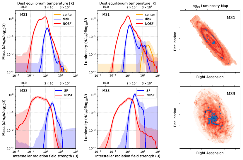
Figure 1 shows our best estimates of dust equilibrium temperature, , equilibrium IR luminosity surface density, , and dust mass surface density, , for each target.111These maps are available in FITS file at https://www.asc.ohio-state.edu/astronomy/dustmaps/ In the SMC, LMC, and M33, we find high dust temperatures in regions of active star formation, consistent with previous works (e.g., Xilouris et al., 2012; Gordon et al., 2014). In M31, the highest dust temperatures coincide with the low dust mass surface density in the inner, bulge-dominated part of the galaxy. Previous work has demonstrated that this hot dust in the inner part of M31 results from heating by the old stellar population (Groves et al., 2012; Draine et al., 2014; Viaene et al., 2014).
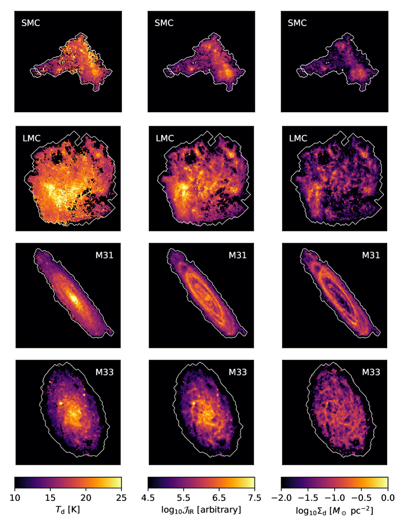
The dust mass surface density maps show the same features as gas mass surface density maps in these galaxies. In the SMC, the ISM material is concentrated along the bar, with an extension to the east into the wing, hosting the bright star-forming complex N83/N84. The LMC shows a prominent ridge of material south of 30 Doradus along the eastern edge of the galaxy and shells through the rest of the galaxy. The dust in M31 is concentrated into a series of rings that may be tightly wound spirals (e.g., Nieten et al., 2006; Gordon et al., 2006). And in M33, the dust mass maps show flocculent spiral structures.
Atomic hydrogen, Hi, makes up most of the neutral ISM in each of our targets. As a result, our maps resemble Hi 21-cm maps of these galaxies (see Kim et al., 1998; Stanimirovic et al., 1999; Staveley-Smith et al., 2003; Braun et al., 2009; Braun, 2012; Koch et al., 2018). In detail, our maps should also reflect the presence of molecular gas and variations of the dust-to-gas ratio. Even accounting for dust-to-gas ratio variations, Figure 1 gives among the most uniform views of the ISM in Local Group galaxies up to date.
The luminosity maps () show the brightest regions where most infrared light comes from. These bright regions are due to high , high , or both (excluding emission from hot, small grains). The star forming regions are still bright because they have both warm and dense . M31 shows distinctive feature, where the bulge (that shows a ‘hole’ in the map) is luminous because of its high .
Based on these maps, we calculate the distributions of dust mass and luminosity as functions of local illuminating radiation field, (in 4.1), and local dust mass surface density, (in 4.2). We compare those distributions in star-forming regions against the rest of area in galaxies in 4.3.
4.1 Distributions of Dust Mass and Luminosity as a Function of Illuminating Radiation Field
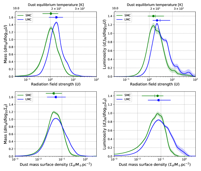
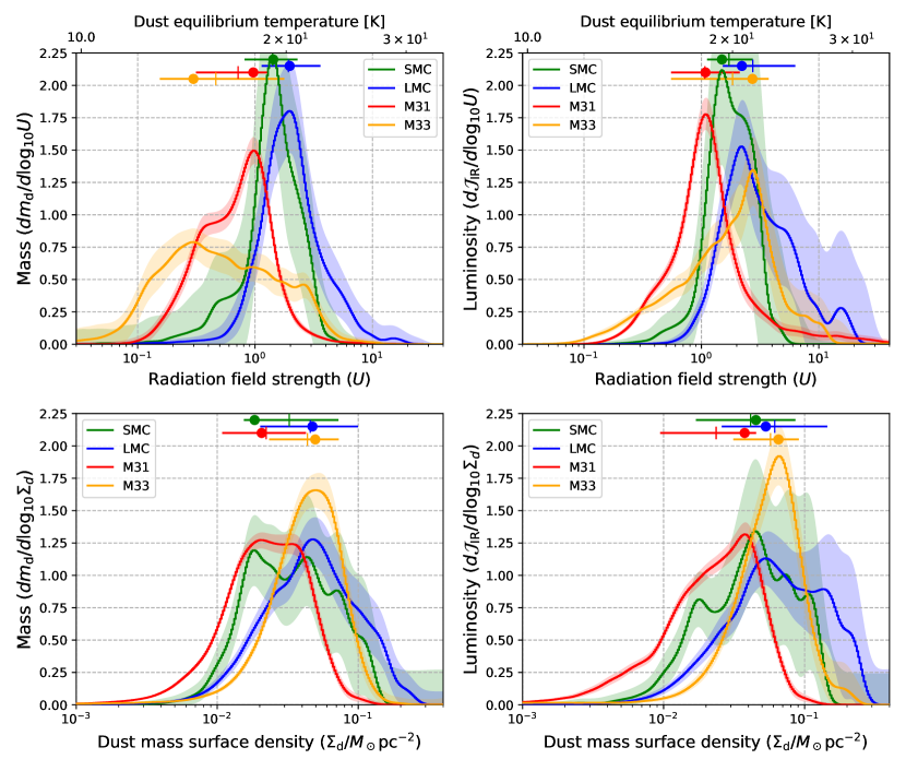
The dust mass distribution as a function of illuminating interstellar radiation field, , strongly affects the integrated SED of a galaxy. Though we cannot measure the sub-resolution scale distribution (e.g., photo-dissociation region or Hii region structure), our maps allow us to measure the dust mass distribution as a function of on galactic scales. We measure and plot these distributions in the top panels of Figure 2 (for the Magellanic Clouds at 13 pc resolution) and the top panels of Figure 3 (for all targets at pc resolution).
Following Dale et al. (2001), we write these distributions as , where is the amount of dust mass heated by within a range of . We choose dex, which is fine enough to capture the details of the distribution function, but not too fine that noise dominates the plots.
We normalize by the total dust mass, , in each galaxy, and define the mass fraction as . Then, the normalized distribution function is
| (12) |
We interpret this normalized distribution function, , as the fraction of the total dust mass per dex of , calculated in a bin with width of and centered at . Less formally, this is the normalized probability density of dust mass as a function of .
Uncertainty: To assess the uncertainty in the measured distributions, we calculate the scatter in the distribution function across a set of 100 realizations of the fitting results (following Gordon et al., 2014; Chiang et al., 2018). We indicate this uncertainty by a shaded area in Figures 2 and 3, which shows the percentile across all realizations. The uncertainty appears larger at 167 pc resolution because lower number of pixels leads to more statistical noise.
To create the realizations, we use the relative likelihoods for each point in our grid space, and randomly draw values from that grid weighted by those relative likelihoods. We repeat this process 100 times for each pixel in each galaxy. This yields 100 realizations of the maps of and for each galaxy.
We construct the distribution functions as described above for each realized map. In each bin of the distribution function, we define the uncertainty as the difference between the and percentile value across all realizations in that bin.
Parameters of the distribution: For each distribution, we measure three quantities described as follows.
-
1.
, defined as the value of that corresponds to the peak of the distribution of mass or luminosity. This is the most common value in the distribution function. It often, but not always lies, near the center of the distribution.
-
2.
, defined as the median value of in the distribution of mass or luminosity.
-
3.
, defined as the logarithmic width in dex of , that covers the 16th-to-84th percentile of mass or luminosity sorted by .
We indicate and for each galaxy by a circle and a tick above the distributions in Figures 2 and 3, and the width as the horizontal line, color coded by galaxy. We record their values in Table 3.
| Galaxies | Resolutions | |||||||||
|---|---|---|---|---|---|---|---|---|---|---|
| Radiation Field | Dust Equilibrium Temperature | Dust Mass Surface Density | ||||||||
| log | log | Width [dex] | [K] | [K] | Width [K] | log | log | Width [dex] | ||
| Distribution of Mass | ||||||||||
| SMC | 13 pc | |||||||||
| LMC | ||||||||||
| SMC | 167 pc | |||||||||
| LMC | ||||||||||
| M31 | ||||||||||
| M33 | ||||||||||
| Distribution of Luminosity | ||||||||||
| SMC | 13 pc | |||||||||
| LMC | ||||||||||
| SMC | 167 pc | |||||||||
| LMC | ||||||||||
| M31 | ||||||||||
| M33 | ||||||||||
Note. — We use Equation 10 to convert to (assuming ). See text for the definition of each parameter. is in pc-2.
4.1.1 Distribution of Dust Mass as a function of Radiation Field
In practice, we calculate by summing the dust mass within each 0.01 dex-wide bin of log. Then, we divide the mass in each bin by the total dust mass in the galaxy and by the 0.01 dex of bin width. For bins of that have no mass in it, we assign the value of in those bins through linear interpolation. Before plotting, we apply Gaussian smoothing with width of five bins. We plot these distributions in the top left panels of Figures 2 and 3.
Because our estimate of depends directly on our best-fit of dust temperature, , via Equation 10, our measured distribution function can also be converted to the distribution of mass as a function of via
| (13) |
In the top left panels of Figures 2 and 3, we show these distribution functions in SMC and LMC at a common 13 pc resolution and in four targets at a common 167 pc resolution.
At 167 pc resolution, M31 has log dex (corresponds to K). This is very close to the Solar neighborhood value of log dex. But, as the top left plot in Figure 3 shows, in M31 lies at the upper end of a wide distribution (i.e. ). Therefore, M31 includes a large amount of mass illuminated by radiation fields below the Solar Neighborhood value. This agrees with the well-known result that the integrated SED in M31 indicates cooler dust temperatures than those in the other Local Group galaxies (e.g., Haas et al., 1998; Groves et al., 2012; Smith et al., 2012; Draine et al., 2014). As Figure 1 shows, much of this cooler material lies in the outer part of the galaxy.
At pc resolution, M33 shows the lowest log in our sample222Keep in mind that we use a constant value of the dust emissivity index, , for all galaxies. Since and are anti-correlated, a lower value of in M33 (; Xilouris et al., 2012) would lead to higher . Conversely, a higher value of in M31 (; Smith et al., 2012) would lead to a lower . ( dex), but this peak lies towards the low end of a wide distribution (i.e. ). M33 has both more mass at high and more mass at low compared to M31 (shown as their horizontal lines), consistent with strong dust temperature gradient (e.g., Xilouris et al., 2012) and extended gas disk in that galaxy (e.g, Koch et al., 2018). Again, Figure 1 shows that the temperature and luminosity have a stronger concentration towards the inner part of the galaxy than the dust mass.
At pc resolution, both Magellanic Clouds show narrower distributions and higher than M31 and M33. The LMC has the highest log (0.30 dex) in our sample, while the SMC has log of 0.16 dex. These values are close to their log values (0.28 dex for LMC and 0.15 dex for SMC). Hence, both galaxies have most of their mass above the Solar neighborhood value (). The LMC includes a significant “tail” toward high , indicating a substantial fraction of its dust mass in high radiation field regions like that around 30 Doradus (see §4.3 and the maps in Figure 1). Compared to the two spirals (M31 and M33), the maps of the Magellanic Clouds show less mass in an extended, cool disk (Figure 1).
4.1.2 Distribution of Luminosity as a function of Radiation Field
We calculate the distribution of equilibrium IR luminosity as a function of , , analogous to the calculation of mass distribution as a function of . We normalize the distribution by the integrated luminosity for the whole galaxy, . The resulting distribution shows the fraction of the equilibrium luminosity per dex of log. We plot these distributions in the top right panels of Figures 2 and 3.
As one might expect, given the dependence of on (Equation 11), higher fraction of the luminosity distributions shift towards higher compared to the mass distributions. This strongly affects in M33, which has the lowest and by mass but has the highest by luminosity (0.44 dex). The other galaxies show modest shifts in and , but the shape of their luminosity distributions around the peak change significantly (compared to that in the mass distribution). In both Magellanic Clouds, the luminosity distribution shows more prominent “bumpy” features at high than in the mass distribution. These reflect large contributions to the luminosity, but smaller contributions to the mass, from hot star forming regions (see §4.3).
At 167 pc resolution, M31 has the lowest log (0.04 dex) and lowest log (0.03 dex), again, close to the Solar neighborhood value. Compared to the mass, less luminosity comes from the low temperature, extended part of the galaxy. This is evident where log for luminosity is , but only for the mass distribution (i.e. lower value of means low- regions contribute more toward the overall distribution). The prominent low- feature in the mass distribution appears dramatically suppressed in the luminosity distribution. Meanwhile, the central part of the distribution (), that maps to the star-forming 10 kpc ring in M31 (Figure 1), increases in prominence. The high- bulge region contributes much more luminosity than mass, but still represents only a small fraction of the galaxy’s total luminosity (1.6%; see §4.3 for detailed discussions).
M33 shows the most striking change between the mass and luminosity distributions. Its shifts from the lowest by mass ( dex) to the highest by luminosity ( dex). Its also increases by 0.60 dex. This reflects the strong dust temperature gradient (Xilouris et al., 2012), which creates a wide range of and , along with the extended gas and dust surface density distributions (Koch et al., 2018). As the maps in Figure 1 show, the mass in M33 extends out to large radii, while the luminosity appears more centrally concentrated, coincides with active star formation (§4.3).
We note that in SMC and LMC, there is a fraction of IR luminosity that comes from dust with K in the star forming regions (high end tail in the top right panel of Figure 2). Even though warm dust component can contribute towards these hot regions, it only contributes a negligible fraction in the mass distribution and lies outside 68% of the mass distribution (top left panel of Figure 2). Hence, the accuracy of our modeling for this warm dust component does not affect the main results of this paper.
4.1.3 The Width of the Distributions
At 167 pc resolution in the Magellanic Clouds and M31, of both the mass and IR luminosity are concentrated within a dex range ( dex, or about a factor of two). In the SMC, the distribution of luminosity appears even narrower, with coming from a dex wide range.
M33 yields the widest distributions of both mass (1.04 dex) and luminosity (0.82 dex) as a function of . As discussed above, these wide distributions reflect the structure of M33 that is visible in Figure 1. High extend into the outer disk, while tends to drop with radius. Meanwhile, in the inner part of the galaxy, multiple knots of star formation activity exhibit both high and .
At pc resolution, available only for the Magellanic Clouds (Figure 2), the distributions appear wider than at pc resolution. These distributions at 13 pc resolution show more material at low radiation fields. This could be expected if the convolution to coarser resolution blurs together warm and cool dust. At their coarser resolution, the light from nearby warmer dust would make it harder to isolate the cool component, leading to the lower amount of low-, low- materials at pc resolution. This idea of relatively “hidden” cool dust, masked by the presence of more luminous material nearby, has appeared many times in the literature (e.g., Galliano et al., 2005). We explore this effect quantitatively in 6.1.
4.2 Distributions of Dust Mass and Luminosity as a Function of Dust Mass Surface Density
We also build the distributions of mass and luminosity as a function of the dust mass surface density, . We plot these and in the lower panels of Figures 2 and 3. We construct these distributions in the same way as those treating as the independent variable (in 4.1), but here, we bin it by log instead of log.
As in 4.1, we characterize the distributions with three parameters, at the peak of the distribution (), the median of the distribution (), and the logarithmic width of the distribution, , defined as the 16th-to-84th percentile range of the distribution. We show these and as the dots and ticks above the distributions in Figures 2 and 3.
4.2.1 Mass Distribution as a function of Dust Mass Surface Density
The bottom left panel in Figure 3 shows the dust mass distribution for our targets at 167 pc resolution. Dust mixed with atomic gas, molecular gas, and even ionized gas are all contribute to these histograms, weighted by the local gas-to-dust ratio. In that sense, this plot also shows the column density distribution of the whole ISM across the Local Group.
Almost all dust mass in all four targets lies in the range pc-2. For a Galactic gas-to-dust ratio (GDR) of , this range equates to a gas mass surface density of pc-2. The metallicities of the LMC, SMC, and M33 are all lower than that in the Milky Way (e.g., Russell & Dopita, 1992; Rosolowsky & Simon, 2008), so the associated range of gas mass surface densities should in fact be more like pc-2. This range is consistent with the fact that the ISM in all of these galaxies is known to be dominated by atomic gas across the disk, with a few dense regions (e.g., the inner part of M33 and the LMC’s ridge region) locally dominated by molecular gas (e.g., Druard et al., 2014; Wong et al., 2011).
The LMC and M33 show similar mass distributions. They exhibit the highest of pc-2 in our sample (their ) and widths of dex. These two dwarf spirals have comparable metallicity, (Russell & Dopita, 1992; Rosolowsky & Simon, 2008), and the distribution appears consistent with dust being mostly mixed with high column density of Hi in both targets.
The SMC shows low and low of and pc-2, respectively. The SMC has a lower metallicity and higher GDR of , compared to those in M33 and the LMC (; Roman-Duval et al., 2014). The lower in the SMC could thus be expected if the gas mass surface density in SMC were comparable to that in LMC. In reality, the SMC’s elongated structure along the line of sight (Stanimirovic et al., 1999; Staveley-Smith et al., 2003) leads to higher Hi column densities than one finds in the other Local Group targets. These effects combine to produce the multi-components distribution (bumps) that mostly overlaps the other targets in the bottom left panel of Figure 3. We emphasize that this overlap is at least partially a coincidence due to the SMC’s orientation.
M31 also shows low and pc-2, again indicating a large amount of mass in an extended disk with relatively low column densities and a GDR that increases with radius (e.g., Draine et al., 2014). Note that M31’s appearance in the plot depends on the substantial correction that we have applied to account for M31’s high inclination (; Corbelli et al., 2010).
4.2.2 Luminosity Distribution as a function of Dust Mass Surface Density
The distribution of luminosity, , shifts toward higher compared to the distribution of mass. The contribution of mass from low is suppressed in the luminosity distribution, changing the shape of distribution in M31 and M33 from symmetric, flat/roundish top, to have narrow peak with tail at low end (positively skewed). The main peak in the luminosity distribution for M31 mostly comes from the star-forming ring and less from the low in the outer disk. The tail towards low shows the influence of the hot bulge.
In the LMC, the distinct components (bumps) in the mass distribution become more pronounce in the luminosity distribution, reflecting the fact that warm dust in high- star-forming regions contribute a lot to the IR luminosity. In the SMC, the distribution changes from negatively skewed in mass to a more symmetric in luminosity, because the high mass surface density regions also tend to have warmer temperature that emits a large fraction of the luminosity.
Because IR luminosity proportional to , the difference between the mass and luminosity distributions implies that temperature correlates with , i.e. part of the luminosity distribution from low is suppressed (because they also have lower ), while luminosity distribution from high is enhanced (because they also have higher ). In 5.1 we show that this appears to be the general case in high signal-to-noise regions, though with some notable exceptions.
4.2.3 Widths Comparisons
At 167 pc resolution, the SMC and LMC have similar width in the distributions of mass and luminosity ( dex), and only slightly larger than the width for M31 and M33 ( dex). This means the SMC and LMC have the largest variations in where 68% of the mass is distributed. As in the mass distribution, the width of luminosity distribution at 167 pc is smaller than that at 13 pc resolution (Table 3) because of convolution between regions with low and high mass surface density.
The shapes of the mass distributions somewhat resemble the distributions of molecular gas mass as a function of in nearby galaxies seen at similar spatial resolution by Sun et al. (2018). They also found signature of multiple components, usually related to distinct dynamical regions (bulge vs. disk). The distributions that we find show more width and more components, perhaps reflecting the wider mixture of environments (e.g. spiral arms and star-forming regions) that is incorporated into our distribution.
In §4.3, we will see that the distributions for any isolated region may appear roughly lognormal in shape. This would agree with the observation that the column density distribution of diffuse neutral gas density in the Milky Way and other Local Group galaxies has a lognormal shape (Berkhuijsen & Fletcher, 2008, 2015; Corbelli et al., 2018). The same shape also emerges from simulations (Wada & Norman, 2007). Making a more rigorous measurement of the shape of the distribution after controlling for regional variations is a subject for future work.
4.2.4 Implications
These mass and luminosity distributions as a function of have two implications: low infrared optical depth and no evidence for opaque Hi, as described below.
Low Infrared Optical Depth: The dust mass surface densities in our targets almost never exceed M⊙ pc-2. Given our adopted value of at 160 µm, this implies that at our resolutions, the optical depth throughout our targets at 100 and 160 µm will be and , respectively. This validates our assumption of optically thin dust that is used in the model (i.e. approximating Equation 1 by Equation 2).
The opacity at µm appears small at both pc (for the Magellanic Clouds) and pc (for all targets). The importance of pressure from reprocessed IR emission scales as the infrared opacity, (e.g., see Thompson et al., 2005), and should exceed the UV-driven radiation pressure when . Thus, we expect radiation pressure from long wavelength infrared photons will contribute an insignificant amount of feedback over essentially all of the area in these targets.
The highest that we observe in the LMC (Figure 2) imply significant opacity at shorter IR wavelengths (e.g., µm). We do not consider emission at these wavelength. However, given the surface densities that we observe and the fact that star forming regions often produce significant emission at these mid-IR wavelengths, our observations are consistent with a significant effect from reprocessed infrared photons in the hottest, highest density parts of our targets (Lopez et al., 2011, 2014). To see this, note that at pc resolution, the LMC by luminosity includes a small, but noticeable, contribution at M⊙ pc-2 (bottom right panel of Figure 2). This M⊙ pc-2 implies of only . If we extrapolate to µm, though, (the extrapolation using is quite approximate but not unreasonable, see Draine 2011). Then, even at the extreme tail of the LMC distribution, we should see a non-trivial, and perhaps even dominant, contribution to the radiation pressure from IR-reprocessed photons.
No Evidence for Hidden Opaque Hi: The modest values that we observe and the smooth appearance of our maps provide evidence against the existence of the patchy, high column density, opaque Hi clouds posited by Braun et al. (2009) and Braun (2012). Braun presented opacity-corrected Hi column density maps in three of our targets; the LMC, M31, and M33. The 21-cm maps that were used to create these Hi maps have comparable angular resolution to our maps. In Braun’s maps, the high gas column density features ( cm-2) appear as small patches sprinkled throughout the maps.
In contrast, our maps do not have a similar patchy appearance, nor do the values of that we find support the presence of gas with column densities approaching cm-2, scattered through the Local Group at this resolution. For the LMC, M33, and M31, we expect the gas to dust ratios of (Leroy et al., 2011; Roman-Duval et al., 2014). In those cases, the that we find corresponds to column densities of cm-2. In order for the opaque Hi features posited by Braun (2012) to exist but not appear in our maps, they would need to be unusually dust poor (i.e. gas to dust ratio of ). To our knowledge, there is no plausible mechanism to produce dense, opaque atomic gas clouds that are preferentially depleted in dust.
Our results do not rule out 21-cm line opacity playing an important role in galaxies, even in these galaxies. More modest effects that operate smoothly across the maps would be hard to distinguish from variations of the gas-to-dust ratio or the presence of CO-dark molecular gas. This issue certainly remains an open topic. Our maps simply do not support with specific structure found by the Braun’s analysis.
4.3 Regional Comparisons
As we see in Figures 2 and 3, there are clear differences in the shape of distribution between mass (left panels) and luminosity (right panels). There are also multiple components in some of the distributions. Comparing the distributions to the maps in Figure 1 suggests that some of these features arise from prominent star-forming regions. Features associated with ongoing massive star formation appear particularly prominent in the luminosity maps of all four targets.
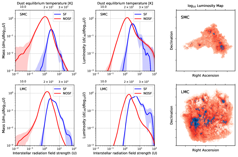
To make a quantitative connection between the structure in the maps and the distribution functions, we divide each galaxy into “star-forming” and “non star-forming” regions and build separate distribution functions for each. We normalize these mass and luminosity distributions by the total mass and total luminosity for the whole galaxy (as in §4.1 and §4.2). For M31, we also build separate distributions for the hot, low central region (inside 1 kpc from the nucleus).
Selection of Regions: We define “star-forming” (SF) regions as areas with Spitzer MIPS (Werner et al., 2004; Rieke et al., 2004) 24 µm intensity MJy sr-1 (shown as the blue regions in the right panels of Figures 4 and 5). This intensity is equivalent to yr-1 kpc-2 (using the calibration from Calzetti et al., 2007). We choose this particular value because it selects the bright regions in the star-forming ring of M31 (Tabatabaei & Berkhuijsen, 2010) and star-forming complexes in the Magellanic clouds and M33 (Relaño & Kennicutt, 2009).
This cutoff also selects the bulge of M31, which shows hot dust (in Figure 1) that Groves et al. (2012) and Smith et al. (2012) argued to be heated by the older stellar population. Therefore, we build separate distributions for this central region (defined as the area within 1 kpc from the nucleus, based on a position angle of from Corbelli et al., 2010).
Resulting Distributions: We show the mass and luminosity distribution functions for star-forming regions (blue) and the rest of area in the galaxy (red) in Figures 4 and 5 (with a log-scale in the vertical axis).
In all four galaxies, both the mass and the luminosity distributions from star-forming regions appear distinct compared to the rest of area in the galaxy. The star forming regions tend to show narrower distributions with a few prominent peaks. As expected, in all four galaxies, the star-forming regions tend to have warmer dust temperature than the rest of area in the galaxy.
Those figures also show that multi-component distributions in Figures 2 and 3 are a result from superimposing physically distinct regions. Star-forming regions, which also tend to be the regions rich in molecular gas, contribute many of the high- and high- features in the full-galaxy distributions. Because the star forming regions have both high and high , they appear even more prominent in the luminosity distribution.
To be concrete, for our adopted definition, the fraction of dust mass that resides in the star forming regions is 10.0% in the SMC, 28.4% in the LMC, 10.2% in M31, and 13.9% in M33. The fraction of luminosity from the star-forming regions is higher, i.e. 24.3% in SMC, 51.4% in LMC, 19.4% in M31, and 44.8% in M33.
The bulge in M31 has higher dust temperature than the star-forming ring or the rest of the galaxy ( K vs. 17 K), but it only captures very small fraction of the total dust mass (). However, this central region (orange histogram in Figure 5) becomes more prominent in the luminosity distribution, with luminosity fraction of . This more prominent contribution in the luminosity distribution, in general, is also true for star-forming regions.
5 Resolved Correlations Among Dust Parameters
5.1 Correlation between Dust Temperature and Mass Surface Density
Both the maps (Figure 1) and the distributions (Figures 2 to 5) suggest a correlation between and , so that high mass surface density regions also tend to be hotter and more luminous. Figure 6 shows this relationship directly, where we plot dust temperature against the dust mass surface density pixel-by-pixel at 13 pc resolution for the Magellanic Clouds and 167 pc resolution for M31 and M33.
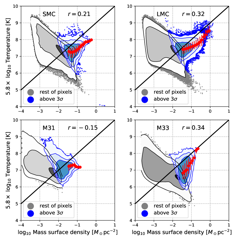
At low signal to noise, we expect the correlated uncertainties to drive an apparent anti-correlation between the best fit and . This reflects that for higher temperature, less mass will be required to produce any given intensity (Equation 5). To suppress this effect, we plot pixels with signal-to-noise less than in either or as gray points and contours. For the rest of this section, we focus our attention on the blue points and contours, which have in both quantities and should be less affected by noise.
Because the maps contain many individual pixels, we use the Gaussian kernel density estimate in Scipy (with bandwidth estimate following Scott, 1992) to calculate the probability density of data points in grids between the minimum and maximum values of those data points. The contours in Figure 6 mark the probability density of 0.005, 0.01, 0.05, and 0.1 data points per grid.
For the SMC, LMC, and M33, the red points show the median temperature in 0.1 dex bin of log, in regions where log. Even though the Spearman (1904) rank correlation coefficient, , is low for all blue points (S/N ), the weak correlation between temperature and dust mass surface density is highly significant because the -value is almost zero. This means warm regions also tend to have high mass surface densities. As we saw in the last section, star forming regions in the maps tend to have both high mass surface density and high temperature.
At some degrees, a correlation between and should be expected on large scales for dust internally heated by star formation. Following Schmidt (1959) and Kennicutt (1998), gas with high mass surface density forms stars more rapidly. If the light from young stars is reprocessed into equilibrium IR emission, then the emergent luminosity should track this star formation. If we approximate and , then the correlation between and appears when the relationship is steeper than linear. Indeed, these galaxies are all mostly Hi-dominated, and the scaling relation does have a super-linear slope (e.g., Bigiel et al., 2008; Schruba et al., 2011), but also has an important dependency on other parameters (Leroy et al., 2008). This one-to-one correlation between and is shown as the black line in Figure 6 (with an arbitrary normalization).
This scaling would be expected for dust heated by star formation. But our sample also includes several cases where this should not be a good approximation. As mentioned several times, the bulge of M31 has hot, low surface density dust. This stands out in the bottom left panel of Figure 6. This dust has been shown to be externally heated by the old stellar population (Groves et al., 2012; Draine et al., 2014).
At pc resolution, the approximation of internal heating may break down due to time evolution of star forming regions. Following Schruba et al. (2010) for M33, at such high resolution the heating sources and gas peaks resolve into discrete features. This effect can also be seen in the Magellanic Clouds (Jameson et al., 2016). In this case, the local will no longer be directly correlated to the amount of heating.
5.2 Intensity at 500 µm and Dust Mass Surface Density
With powerful sub-millimeter telescopes like ALMA, it has become common to estimate the dust mass from only one or a few measurements on the Rayleigh-Jeans tail of the SED. This approach assumes a dust temperature, either implicitly or explicitly. Here, we compare from our five bands fitting, which leverages information from the µm SED to the monochromatic intensity at µm. This offers a check on the reliability of sub-mm intensities as a dust mass tracer.
Figure 7 shows the correlation between resolved and over three orders of magnitude in both axes. We only select pixels above uncertainty for both and . Contours show the density of data points, generated using the Gaussian kernel density estimate with a kernel size of dex. In each panel, the diagonal lines show relations with power law index of 1 with normalization set by the median of measured for each galaxy. The value of this median ratio is for the LMC, for the SMC, for M31, and for M33, where is in units of pc-2 and is in units of MJy sr-1. The lower and upper limits are the 16th and 84th percentiles, respectively. Among all of our targets, the variation of this ratio roughly agrees with the simple expectation based on our measured variations in .
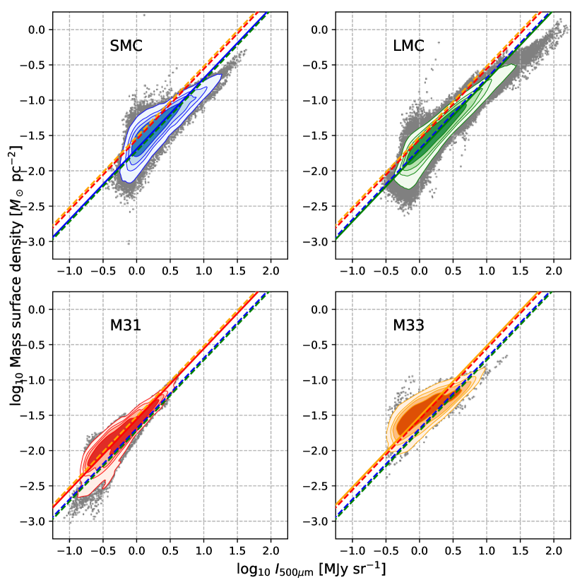
Both contours of M31 and M33 show a shallow slope in Figure 7 (compared to one-to-one relation). These reflect the temperature gradients discussed above (Xilouris et al., 2012). In these galaxies, taking to linearly trace would give a bias so that the dust appears to be more centrally concentrated than it actually is. In other words, the temperature gradient causes the inner part of M33, and the star-forming ring and bulge of M31, to glow more brightly than the rest of the galaxy, while the cooler outer regions are fainter. This effect appears less pronounced in the Magellanic Clouds at high resolution.
Overall, this exercise confirms that predicts within an accuracy of about for our sample, but with systematic biases in the two disk galaxies with temperature gradients. We emphasize that this only tests the ability to recover the dust surface density. We have taken no account here for variations in the gas-to-dust ratio.
5.3 Infrared Color and Temperature
Finally, we compare the 100-to-250 µm or 100-to-350 µm infrared color to the from our five band fits. This allows us to check how well our model reproduces this IR color and to verify how well we would have predicted from only a single band ratio. We focus on and as colors because those wavelengths bracket the peak of the dust SED at µm.
Figure 8 shows as a function of IR color for data with in both color and temperature. Contours indicate data density as in §5.2. We also plot the relation between temperature and colors as expected from the modified blackbody models with 1.4, 1.8, and 2.2.
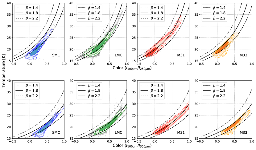
The data broadly follow the model, although with some notable deviations. The plots suggest that LMC and M33 may be better described by closer to than our adopted . Both the SMC and the LMC show points covering a range of , with the regions with redder IR color are more consistent with higher , while the rest of the pixels is in good agreement with our adopted value of . Note that despite the shift in , these features are as likely come from multiple dust populations unresolved by our observation (mixing of multiple populations within the beam) and the influence of out-of-equilibrium heating at short wavelengths, so that they appear as variations in dust properties (changing ). These reflect deviations from our model. The strength of this feature in the SMC appears consistent with previous observations that hot, small grains contribute heavily to the SED in this galaxy (e.g., Bot et al., 2004).
Lastly, we note that in the range of K, the modified blackbody models still show a curvature in the colortemperature relation (black curves in Figure 8). This means we can still constrain the dust temperature well within that temperature range. A vertical slope would mean the temperature loses its sensitivity to the IR color (i.e. approaching Rayleigh-Jeans tail), and this is clearly not the case in our study. Therefore, the high-temperature tail in the distributions (Figure 2) is real.
6 The Dependence of Dust Mass and Temperature on Physical Resolutions
6.1 Dust Temperature as a Function of Physical Scale
We study four of the closest star-forming galaxies at the diffraction limit of the best infrared telescope to date. This high physical resolution is not available for distant galaxies. Still, as discussed in §1, there remains considerable interest in using dust as a tracer of gas in more distant systems. Therefore, we explore the effects of physical resolution on the derived dust temperature and mass.
We choose the weighting methodology (described below) to create coarser resolution maps. This is different than convolving the SED first and then fitting that convolved SED. The reason behind this choice is we lose the background area gradually in the coarser resolution maps. This would make the covariance matrix calculation (Equation 7) becomes difficult and leading to non-robustness of the fitting results of the convolved SED (see Appendix A).
Method: Observing at coarse resolution tends to emphasize the sources of luminosity, rather than mass. To investigate the effects of resolution, we compare our high resolution results to what we would derive from luminosity (rather than mass) weighted averages at some coarser resolutions. We compare any results at coarser resolutions to the mass-weighted average at the finest resolution, because we consider the latter as a quantity closest to the true temperature from the majority of dust mass.
Specifically, we calculate the luminosity-weighted temperature, , and the luminosity-weighted mass surface density, , at resolutions coarser than our original maps. To calculate , we begin with our highest resolution map, weight that map by luminosity, convolve that map to lower resolution, and then, divide the result by the convolved luminosity map. Mathematically, this is expressed as
| (14) |
where is a quantity proportional to the equilibrium dust luminosity per unit area in the highest resolution map (as defined by Equation 11), denotes convolution, and is the Gaussian kernel to convolve from the finest resolution to the target coarser resolution.
Similarly, we calculate the luminosity-weighted mass surface density, , via
| (15) |
In Equations 14 and 15, we calculate and for each pixel at coarser resolution. To represent the temperature for a single galaxy, we also calculate the mean value of temperature (weighted by mass) at each resolution via
| (16) |
Similarly, the luminosity-weighted mean temperature for a single galaxy at coarser resolution is
| (17) |
Here, the sum runs over all pixels inside the region of interest.
As we have seen in 4.3, weighting by luminosity leads to higher because more weight is attached to hot, high luminosity star-forming regions. Because we use the luminosity-weighting to convolve the data to coarser resolutions, information below the resolution is irrevocably “washed out.” Comparing mass-weighted results at different resolutions shows how much this “sub-resolution” luminosity-weighting changes our inferences about the dust temperature and mass. This gives us an empirical estimate of how much the implicit luminosity-weighting in low resolution observations will wash out information on the true dust mass.
Results for temperature: In Figure 9, we plot (black dots) for each galaxy as a function of physical resolution. We also mark at the finest resolution as blue lines. This is the quantity that is closest to the true mass-weighted mean of temperature in a galaxy. Any other measurements should be compared to this line. Due to different physical sizes among galaxies, LMC and SMC are convolved to resolutions from pc to pc, while M31 and M33 are convolved to resolutions from pc to kpc.
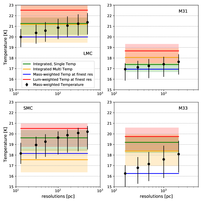
In general, rises as the resolution becomes coarser. This has the expected sense, because convolving cool, low surface density regions with warm, high surface density regions would bias towards higher temperatures. We already saw an indication of this effect when comparing the distributions of mass by radiation field at pc and pc resolution for the Magellanic Clouds (Figures 2 and 3).
This trend of with spatial resolution is weakest in M31; the inferred mean temperature only changes by K as we blur the maps by a factor of in resolution. We identify two likely causes. First, we see a weak correlation between temperature and mass surface density in Figure 6. Second, much of the variation in temperature occurs radially on kpc scales or larger, so that blurring together the distinct physical conditions is less of an issue in M31.
The SMC and M33 show the largest increases in with coarser spatial resolutions. The implied temperature in both galaxies increases by K as the resolution degrades by a factor of . The LMC shows an intermediate case. We again attribute the magnitude of this resolution effect to the spatial structure and dynamic range in temperature variations in the galaxy. In general, the smaller, more star-formation dominated systems show more systematic effects, and more information loss, from blurring the data.
The red and blue horizontal lines in Figure 9 indicate the luminosity weighted temperature, , and mass-weighted temperature, , respectively, at the finest resolution. By construction, the black point lies on the blue line at the finest resolution. As we blur the galaxy towards a single resolution element, the black points should approach the red line. The difference between the red and blue lines shows the maximum effect of interchanging luminosity and mass weighting. This difference is K, or about change in , or a factor of change in .
Implication for the total mass measurement: Luminosity weighting tends to bias towards higher temperature. An overestimate of temperature will lead to an underestimate of the mass. To see this, consider a point on the Rayleigh-Jeans tail, for which . As the luminosity-weighting biases toward higher temperature, it will also lead to an underestimate of the mass.
To first order, the mass will be biased low by the same fraction as the temperature is biased high. This is change over the range of resolutions that we study. However, this does not capture the effects of any distributions of mass or temperature beneath our finest resolution (13 pc for Magellanic Clouds and 167 pc for M31 and M33).
For the LMC, Galliano et al. (2011) considered exactly this effect and estimated that the mass inferred from the integrated SED is biased low by . They included shorter wavelength bands than what we study here, which likely accounts for that stronger bias than what we found. The effect of luminosity weighting should be stronger for these shorter wavelength bands because they are more sensitive to the dust temperature.
In general, following Dale et al. (2001), accounting for distributions of temperatures in modeling the SED is crucial for a correct mass estimation. Emphasizing longer wavelengths, as we do here, somewhat diminishes this resolution effect. Even at 13 pc resolution, mass estimations in SMC and LMC are still less accurate because a significant portion of blending populations (unresolved by our study) must still occur even below that resolution.
6.2 Fits to the Integrated SED and Comparison with Resolved Mapping
We also fit the integrated SED, equivalent to unresolved observation. Even in the local universe, this is often the only type of measurement available for a galaxy. In particular, poor resolution options remain the main way to study high redshift galaxies (e.g., Magdis et al., 2010, 2012; Genzel et al., 2015) and there has been some controversy about how to best estimate dust mass in these galaxies. Here, following Galliano et al. (2011), we check how the temperature and dust mass derived from the integrated SED compared to those derived from the highly resolved maps.
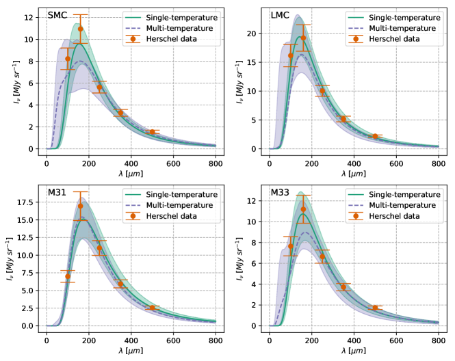
We calculate the integrated SED by taking the mean surface brightness within the region of interest. We report the mean intensity for each target at each band in Table 4. We also note the averaging area, in steradians. To calculate the integrated SED in units of specific flux, we multiply the area by the intensities. Then, we fit the SED with two approaches; single-temperature and multi-temperature modified blackbodies. Figure 10 shows these integrated SEDs as red points, along with the best-fit models (curves). Uncertainty in the best-fit models, visualized by drawing 100 realizations in proportion to their likelihood, are shown as shaded areas.
In Table 4, we compare the dust temperature and total mass between galaxies from three different approaches; (1) integrated SED, fitted using single-temperature modified blackbody, (2) integrated SED, fitted using multi-temperature modified blackbody, and (3) the mass-weighted mean of temperature, , calculated from the finest resolution map.
Single-Temperature Model: First, we use the same single-temperature modified blackbody model as adopted for the resolved observations. The best-fit models are shown as the solid green curves in Figure 10. Despite the simplicity of our model, it offers a good fit to the integrated SED of each galaxy. Mathematically, this is different than the luminosity-weighted mean of temperature, , because in the integrated SED, we take average of intensity without any weighting. Therefore, we do not expect to be the same as the temperature derived from the integrated SED fitting (red vs. green lines in Figure 9).
| Galaxies | Flux Density [ Jy] | Dust Equilibrium Temperature [K] | Total Dust Mass [] | ||||||||
|---|---|---|---|---|---|---|---|---|---|---|---|
| 100 µm | 160 µm | 250 µm | 350 µm | 500 µm | Single | Multi | Resolved | Single | Multi | Resolved | |
| SMC | |||||||||||
| LMC | |||||||||||
| M31 | |||||||||||
| M33 | |||||||||||
The expected value of from fitting these integrated fluxes are shown as the green lines in Figure 9. Dust temperature from fitting the integrated SED is higher than the mass-weighted temperature of the most highly resolved observations. This means the unresolved observations would overestimate the temperature of the majority of the dust by K or a factor of for 18 K temperature. If using a single flux at 500 µm to measure the dust mass (Equation 1 in Scoville et al., 2014), this translates to an underestimate of dust mass also by for an object with 18 K dust temperature.
Multi-temperature Model: We also fit the integrated SED by adopting a sub-resolution multi-temperature distribution in the form of (for ; Draine & Li, 2007)
| (18) |
where is Dirac’s delta function. Here, a fraction of the dust mass within a resolution element is heated by a power law distribution field between and , while the rest is heated by the ambient ISRF of .
We use the same grid-based fitting procedure as before (§3.2). The grid for is from to with an increment of , the grid for log is from to with an increment of , and the grid for log from to with an increment of . The grids for dust temperature and mass surface density are the same as in the single temperature modified blackbody model (§3.2). The value of is fixed at . The adoption of this value does not affect the outcome of fitting parameters.
The best-fit models are shown as the dashed purple curves in Figure 10. The expected values for , , and are listed in Table 5. The value of represents the ambient ISRF that illuminate the majority () of dust mass. Hence, it is not surprising that it is highest in the LMC, in general agreement with the distribution of dust mass as a function of (4.1). The rest of dust mass (a fraction of ) is heated by ISRF in the range between and .
| Galaxies | log | ||
|---|---|---|---|
| [dex] | [%] | ||
| SMC | |||
| LMC | |||
| M31 | |||
| M33 |
The value of shows the relative contribution of dust mass at the high-end tail of , compared to that in the low-end tail of , where . A shallower slope (lower ), such as in the SMC and M33, means the low-end tail of (originated from star-forming regions) contributed more to the dust mass spectrum between and . Hence, this multi-temperature fit is not only adding free parameters, but also physically more reasonable than a single-temperature fit of modified blackbody.
Following Draine & Li (2007), we calculate the mass-weighted mean of via
| (19) |
Then, we convert to the dust temperature by inverting Equation 10.
Comparison between methods: In SMC and M33, the temperature derived from integrated SED multi-temperature is lower than those derived from the integrated SED single-temperature model by K, while the opposite happens in M31. The best-fit temperature from two methods above matches in LMC. Compared to , the temperature derived from integrated SED (using both single- and multi-temperature model) has higher temperature than by K (except for integrated multi-temperature in the SMC). This difference is because the integrated SED convolves together many regions so it is biased toward warm regions (for single-temperature model), and the limitation in modeling the integrated SED to recover the true distribution of as seen in the highly resolved map (for multi-temperature model).
For the total dust mass, all three methods (integrated SED with single-temperature, integrated SED with multi-temperature, and by summing mass from all pixels in the finest resolution map) agree remarkably well in M31. In the Magellanic Clouds and M33, the mass from the finest resolution map is in between results from the single- and multi-temperature methods. In the Magellanic Clouds, the single-temperature method gives better agreement (but with lower mass) compared to the total mass from resolved map, while in M33, we find better agreement (but with higher mass) between the total masses from multi-temperature method and the resolved map.
7 Summary
Using the archival Herschel maps covering from to µm and a fitting algorithm developed by Gordon et al. (2014) and implemented by Chiang et al. (2018), we derive maps of equilibrium dust temperature (), dust mass surface density (), and equilibrium infrared luminosity () for four Local Group galaxies: the Small and Large Magellanic Cloud, M31, and M33. We show these maps, which we make publicly available, in Figure 1. We construct the maps at pc resolution, the common physical resolution available for the Magellanic Clouds, and pc resolution, the common physical resolution available for all four targets.
We use these maps to measure how the dust mass and luminosity are distributed as functions of (or equivalently, the interstellar radiation field strength, ), and , in each target. We show these distributions in Figures 2 and 3.
Based on these calculations, we gauge the median dust temperatures and surface densities by mass and luminosity and note the characteristic widths of these distributions. We report these values in Table 3. We highlight the following key points.
-
1.
At pc resolution, the distribution of dust mass as a function of radiation field implies a median K. If we instead consider the distribution of luminosity, the median appears higher, K. On average, the peak of weighting by luminosity is only K higher than the peak of weighting by mass, but in M33, this shift is about K, reflecting the strong radial structure in that galaxy.
-
2.
At pc resolution, of the dust mass is spread over dex in radiation field, . The luminosity spans a lower range, dex. Again, the strong radial structure and extended disk in M33 lead to a wider distribution, dex, than we see in the other galaxies ( dex).
-
3.
Also at pc resolution, the dust mass as a function of surface density (i.e., the dust mass surface density PDF) has median value to , i.e., M⊙ pc-2. This agrees well with observation that the neutral ISM in all of our targets is mostly Hi with dust to gas ratios of a few hundred to a thousand. The median for the distribution of luminosity is usually dex lower than the distribution by mass.
- 4.
Both the dust mass and luminosity PDFs show significant structure. This structure relates to features visible in the temperature, luminosity, and surface density maps. For example, M33’s strong radial temperature gradient leads to a wide, multi-component distribution in dust mass as a function of temperature. Similarly, M31’s star-forming ring and hot but low-surface density bulge region manifest as clear features in the distribution.
To further quantify how regional features contribute to the global distribution, we identify the active star-forming part of each galaxy and construct a separate distribution for this region and the quiescent region (Figures 4 and 5). We find the following.
-
5.
As expected, the star-forming parts of galaxies have warmer dust temperature and higher dust mass surface density than the rest of the regions in the galaxy. In our sample, the notable exception is M31, where dust in the central region is heated by older stellar populations (Groves et al., 2012; Smith et al., 2012). This dust stands out in our sample because of its combination of low mass surface density but high dust temperature.
-
6.
Although these star-forming regions contribute a small fraction to the total dust mass (), they produce a significant fraction of the equilibrium luminosity in the infrared ().
Furthermore, we see a more general form of these results by directly plotting the correlation between and for the points with high (Figure 6). We find the following.
-
7.
Dust temperature () correlates with dust mass surface density () in SMC, LMC, and M31 (Spearman rank correlation coefficients are weak, but highly significant). In M31, a weak correlation is evident in the dust associated with the star-forming ring, but the hot, low surface density bulge dust heated by the old stellar population leads to an overall anti-correlation between and .
-
8.
Very roughly, the sense of the correlation between and agrees with expectations from an approximately quadratic gas-star formation scaling relation (), as might be roughly expected in the Hi-dominated regime appropriate for our targets.
The Herschel Space Observatory observed the Local Group galaxies at high physical resolutions. We compare our results to those expected for the same galaxies at farther distances (higher redshift) by progressively convolving the galaxies to coarser resolutions. We find the following.
-
9.
The luminosity-weighted mean temperature typically exceeds the mass-weighted mean temperature, , by K, an increase of about 10% (or about a factor of in ). Progressively blurring the maps with a luminosity weighting causes the low resolution to increase, approaching this higher value (Figure 9).
-
10.
The best-fit temperature derived from the integrated SED (equivalent to unresolved source) is higher than from the finest resolution map (Table 4). This bias is somewhat reduced when a sub-resolution multi-temperature distribution (e.g., the approach in Dale et al., 2001; Draine & Li, 2007) is used.
-
11.
Both points above quantify how severely the temperature from low resolution IR-SED fitting in distant galaxies may overestimate their true mass-weighted mean temperature. As a consequence, the inferred total dust mass in distant galaxies would be underestimated. This is particularly important when the gas mass is determined based on the dust mass.
Lastly, we compare our five-bands fitting results to those that would be obtained by using only one or two bands, as is now commonly required with ALMA (Scoville et al., 2014). We test how the 500 µm intensity, , performs as a tracer for dust mass surface density, . We also test how well our best-fit matches individual infrared color ( or ). We find the following.
-
11.
A median radio of over can recover the trend between and in our data (Figure 7). There are two subtleties. First, there is offset in this median ratio from galaxy-to-galaxy. Second, real temperature variations, e.g., as seen in M33 gradient, lead to systematic bias and a modestly sublinear slope between and . The sense is that without accounting for radial trend in dust temperature, one would estimate that dust in M33 to be more confined to the galaxy center than it actually is.
-
12.
Although it is an implication of our modeling method to determine the dust temperature, the modified black-body model with a single-temperature and a constant emissivity index, , can adequately relate the infrared color and dust temperature (Figure 8), provided that the wavelengths (used as the IR-color) bracket the peak wavelength of the cold dust emission. We observe scatter in this color–temperature relation, particularly in the low temperature. Also, the color–temperature relation in the SMC looks steeper than the prediction from the model, probably due to variation of from region-to-region (Gordon et al., 2014).
We make the maps of dust temperature and mass surface density in the FITS file to be publicly available at https://www.asc.ohio-state.edu/astronomy/dustmaps.
Appendix A Challenge in comparing across physical resolutions
One challenge in fitting the dust properties across physical resolutions is computing the covariance matrix of the background fluxes (3.2) for the low-resolution images. The convolution process blurs the image. Therefore, to conserve flux from a galaxy, the background area decreases and the region of interest area increases in the low resolution maps. This means we can only compute the covariance matrix of background flux correctly down to certain resolution. In this study, this lower limit in resolution is selected to be where there are at least ten resolution elements across the target image.
It is shown in Chiang et al. (2018) that the choice of covariance matrix heavily affects the results of fitting. Thus without the covariance matrix of background fluxes, we are unable to fit dust properties at coarser resolutions. Several attempts have been made to extrapolate the covariance matrix to coarser resolutions. So far, none of the methods we try are proved to give the correct matrix mainly due to two reasons. (1) The background flux consists of both random noise and real signal from background objects. (2) The observed correlations between Herschel bands are not constant across resolutions. Whether it is possible to extrapolate the covariance matrix for low-resolution images from high-resolution images remains an open question for future study.
References
- Aniano et al. (2011) Aniano, G., Draine, B. T., Gordon, K. D., & Sandstrom, K. 2011, PASP, 123, 1218
- Balog et al. (2014) Balog, Z., Müller, T., Nielbock, M., et al. 2014, Experimental Astronomy, 37, 129
- Bendo et al. (2017) Bendo, G., Conversi, L., Fulton, T., et al. 2017, SPIRE Handbook v3.1, Herschel Science Centre, Paris, France, hERSCHEL-DOC-0798
- Berkhuijsen & Fletcher (2008) Berkhuijsen, E. M., & Fletcher, A. 2008, MNRAS, 390, L19
- Berkhuijsen & Fletcher (2015) —. 2015, MNRAS, 448, 2469
- Bianchi (2013) Bianchi, S. 2013, A&A, 552, A89
- Bigiel et al. (2008) Bigiel, F., Leroy, A., Walter, F., et al. 2008, AJ, 136, 2846
- Boquien et al. (2011) Boquien, M., Calzetti, D., Combes, F., et al. 2011, AJ, 142, 111
- Bot et al. (2004) Bot, C., Boulanger, F., Lagache, G., Cambrésy, L., & Egret, D. 2004, A&A, 423, 567
- Braine et al. (2010) Braine, J., Gratier, P., Kramer, C., et al. 2010, A&A, 518, L69
- Braun (2012) Braun, R. 2012, ApJ, 749, 87
- Braun et al. (2009) Braun, R., Thilker, D. A., Walterbos, R. A. M., & Corbelli, E. 2009, ApJ, 695, 937
- Calzetti et al. (2007) Calzetti, D., Kennicutt, R. C., Engelbracht, C. W., et al. 2007, ApJ, 666, 870
- Chastenet et al. (2017) Chastenet, J., Bot, C., Gordon, K. D., et al. 2017, A&A, 601, A55
- Chiang et al. (2018) Chiang, I.-D., Sandstrom, K. M., Chastenet, J., et al. 2018, ApJ, 865, 117
- Clements et al. (2010) Clements, D. L., Dunne, L., & Eales, S. 2010, MNRAS, 403, 274
- Corbelli et al. (2018) Corbelli, E., Elmegreen, B. G., Braine, J., & Thilker, D. 2018, A&A, 617, A125
- Corbelli et al. (2010) Corbelli, E., Lorenzoni, S., Walterbos, R., Braun, R., & Thilker, D. 2010, A&A, 511, A89
- Dale & Helou (2002) Dale, D. A., & Helou, G. 2002, ApJ, 576, 159
- Dale et al. (2001) Dale, D. A., Helou, G., Contursi, A., Silbermann, N. A., & Kolhatkar, S. 2001, ApJ, 549, 215
- Draine (2003) Draine, B. T. 2003, ARA&A, 41, 241
- Draine (2011) —. 2011, Physics of the Interstellar and Intergalactic Medium
- Draine & Li (2007) Draine, B. T., & Li, A. 2007, ApJ, 657, 810
- Draine et al. (2007) Draine, B. T., Dale, D. A., Bendo, G., et al. 2007, ApJ, 663, 866
- Draine et al. (2014) Draine, B. T., Aniano, G., Krause, O., et al. 2014, ApJ, 780, 172
- Druard et al. (2014) Druard, C., Braine, J., Schuster, K. F., et al. 2014, A&A, 567, A118
- Dunne & Eales (2001) Dunne, L., & Eales, S. A. 2001, MNRAS, 327, 697
- Freedman et al. (1991) Freedman, W. L., Wilson, C. D., & Madore, B. F. 1991, ApJ, 372, 455
- Fritz et al. (2012) Fritz, J., Gentile, G., Smith, M. W. L., et al. 2012, A&A, 546, A34
- Galliano et al. (2005) Galliano, F., Madden, S. C., Jones, A. P., Wilson, C. D., & Bernard, J.-P. 2005, A&A, 434, 867
- Galliano et al. (2011) Galliano, F., Hony, S., Bernard, J.-P., et al. 2011, A&A, 536, A88
- Genzel et al. (2015) Genzel, R., Tacconi, L. J., Lutz, D., et al. 2015, ApJ, 800, 20
- Gordon et al. (2006) Gordon, K. D., Bailin, J., Engelbracht, C. W., et al. 2006, ApJ, 638, L87
- Gordon et al. (2014) Gordon, K. D., Roman-Duval, J., Bot, C., et al. 2014, ApJ, 797, 85
- Graczyk et al. (2014) Graczyk, D., Pietrzyński, G., Thompson, I. B., et al. 2014, ApJ, 780, 59
- Griffin et al. (2010) Griffin, M. J., Abergel, A., Abreu, A., et al. 2010, A&A, 518, L3
- Groves et al. (2012) Groves, B., Krause, O., Sandstrom, K., et al. 2012, MNRAS, 426, 892
- Haas et al. (1998) Haas, M., Lemke, D., Stickel, M., et al. 1998, A&A, 338, L33
- Jameson et al. (2016) Jameson, K. E., Bolatto, A. D., Leroy, A. K., et al. 2016, ApJ, 825, 12
- Jenkins (2009) Jenkins, E. B. 2009, ApJ, 700, 1299
- Kelly et al. (2012) Kelly, B. C., Shetty, R., Stutz, A. M., et al. 2012, ApJ, 752, 55
- Kennicutt (1998) Kennicutt, Jr., R. C. 1998, ApJ, 498, 541
- Kim et al. (1998) Kim, S., Staveley-Smith, L., Dopita, M. A., et al. 1998, ApJ, 503, 674
- Klein (2014) Klein, C. R. 2014, PhD thesis, University of California, Berkeley
- Koch et al. (2018) Koch, E. W., Rosolowsky, E. W., Lockman, F. J., et al. 2018, MNRAS, 479, 2505
- Leroy et al. (2008) Leroy, A. K., Walter, F., Brinks, E., et al. 2008, AJ, 136, 2782
- Leroy et al. (2011) Leroy, A. K., Bolatto, A., Gordon, K., et al. 2011, ApJ, 737, 12
- Lopez et al. (2011) Lopez, L. A., Krumholz, M. R., Bolatto, A. D., Prochaska, J. X., & Ramirez-Ruiz, E. 2011, ApJ, 731, 91
- Lopez et al. (2014) Lopez, L. A., Krumholz, M. R., Bolatto, A. D., et al. 2014, ApJ, 795, 121
- Magdis et al. (2010) Magdis, G. E., Elbaz, D., Hwang, H. S., et al. 2010, MNRAS, 409, 22
- Magdis et al. (2012) Magdis, G. E., Daddi, E., Béthermin, M., et al. 2012, ApJ, 760, 6
- Mathis et al. (1983) Mathis, J. S., Mezger, P. G., & Panagia, N. 1983, A&A, 128, 212
- McMullin et al. (2007) McMullin, J. P., Waters, B., Schiebel, D., Young, W., & Golap, K. 2007, in Astronomical Society of the Pacific Conference Series, Vol. 376, Astronomical Data Analysis Software and Systems XVI, ed. R. A. Shaw, F. Hill, & D. J. Bell, 127
- Meixner et al. (2013) Meixner, M., Panuzzo, P., Roman-Duval, J., et al. 2013, AJ, 146, 62
- Nieten et al. (2006) Nieten, C., Neininger, N., Guélin, M., et al. 2006, A&A, 453, 459
- Paturel et al. (2003) Paturel, G., Petit, C., Prugniel, P., et al. 2003, A&A, 412, 45
- Pilbratt et al. (2010) Pilbratt, G. L., Riedinger, J. R., Passvogel, T., et al. 2010, A&A, 518, L1
- Planck Collaboration et al. (2011) Planck Collaboration, Abergel, A., Ade, P. A. R., et al. 2011, A&A, 536, A25
- Poglitsch et al. (2010) Poglitsch, A., Waelkens, C., Geis, N., et al. 2010, A&A, 518, L2
- Relaño & Kennicutt (2009) Relaño, M., & Kennicutt, Jr., R. C. 2009, ApJ, 699, 1125
- Rieke et al. (2004) Rieke, G. H., Young, E. T., Engelbracht, C. W., et al. 2004, ApJS, 154, 25
- Roman-Duval et al. (2014) Roman-Duval, J., Gordon, K. D., Meixner, M., et al. 2014, ApJ, 797, 86
- Rosolowsky & Simon (2008) Rosolowsky, E., & Simon, J. D. 2008, ApJ, 675, 1213
- Russell & Dopita (1992) Russell, S. C., & Dopita, M. A. 1992, ApJ, 384, 508
- Schmidt (1959) Schmidt, M. 1959, ApJ, 129, 243
- Schruba et al. (2010) Schruba, A., Leroy, A. K., Walter, F., Sandstrom, K., & Rosolowsky, E. 2010, ApJ, 722, 1699
- Schruba et al. (2011) Schruba, A., Leroy, A. K., Walter, F., et al. 2011, AJ, 142, 37
- Scott (1992) Scott, D. W. 1992, Multivariate Density Estimation
- Scoville et al. (2014) Scoville, N., Aussel, H., Sheth, K., et al. 2014, ApJ, 783, 84
- Smith et al. (2012) Smith, M. W. L., Eales, S. A., Gomez, H. L., et al. 2012, ApJ, 756, 40
- Spearman (1904) Spearman, C. 1904, The American Journal of Psychology, 15, 72
- Stanimirovic et al. (1999) Stanimirovic, S., Staveley-Smith, L., Dickey, J. M., Sault, R. J., & Snowden, S. L. 1999, MNRAS, 302, 417
- Staveley-Smith et al. (2003) Staveley-Smith, L., Kim, S., Calabretta, M. R., Haynes, R. F., & Kesteven, M. J. 2003, MNRAS, 339, 87
- Subramanian & Subramaniam (2012) Subramanian, S., & Subramaniam, A. 2012, ApJ, 744, 128
- Sun et al. (2018) Sun, J., Leroy, A. K., Schruba, A., et al. 2018, ApJ, 860, 172
- Tabatabaei & Berkhuijsen (2010) Tabatabaei, F. S., & Berkhuijsen, E. M. 2010, A&A, 517, A77
- Thompson et al. (2005) Thompson, T. A., Quataert, E., & Murray, N. 2005, ApJ, 630, 167
- van der Marel & Cioni (2001) van der Marel, R. P., & Cioni, M.-R. L. 2001, AJ, 122, 1807
- Viaene et al. (2014) Viaene, S., Fritz, J., Baes, M., et al. 2014, A&A, 567, A71
- Vilardell et al. (2010) Vilardell, F., Ribas, I., Jordi, C., Fitzpatrick, E. L., & Guinan, E. F. 2010, A&A, 509, A70
- Wada & Norman (2007) Wada, K., & Norman, C. A. 2007, ApJ, 660, 276
- Werner et al. (2004) Werner, M. W., Roellig, T. L., Low, F. J., et al. 2004, ApJS, 154, 1
- Wong et al. (2011) Wong, T., Hughes, A., Ott, J., et al. 2011, ApJS, 197, 16
- Xilouris et al. (2012) Xilouris, E. M., Tabatabaei, F. S., Boquien, M., et al. 2012, A&A, 543, A74