Could the Hilbert Space Be a Smaller Place?
A Neural Network Perspective

Abstract

In quantum many-body problems, one of the main difficulties comes from the description of non-negligible interactions which require, at least in principle, an exponential amount of information. Recently, in the context of spin glasses and Boltzmann machines, it has been demonstrated that systematic machine learning of the wave function can reduce these issues to a tractable computational problem. In this work, we apply this approach to a different situation, i.e. the problem of finding the ground state of a given quantum system made of electrons, entirely described by its Hamiltonian operator, and by utilizing feedforward neural networks. Although still in the shape of a proof of concept, one can already observe that this seminal idea is able to substantially simplify the complexity of this peculiar, and important, problem.

1 Introduction

The motto ”Hilbert space is a big place” is well known by the practitioners of quantum mechanics. It describes, in a few words, how the complexity of this space increases rapidly when approached either theoretically or numerically. The purpose of this paper is to show that neural networks can help to reduce such difficulties. Specifically, we focus on the problem of finding the ground state of typical quantum systems such as one or more electrons in the presence of a given external potential. This is twofold: it shows that single-electron problems can be efficiently dealt by neural networks, and that it also can be applied to the context of quantum many-body problems in both density functional theory and first-principle approaches. This is a problem which is not only of theoretical importance, but also of technological, economical and even sociological relevance. In fact, quantum mechanics is the theory which has made possible things such as laser beams, integrated circuits, microprocessors, and has even improved our comprehension of the DNA.

Recently, Carleo et al. introduced a very general method based on neural networks to represent the state of a quantum system. As a practical instance, this approach has been applied to the specific case of Boltzmann machines representing the state of a spin glass [1], [2]. Although at a seminal stage, this method proves to be very robust and accurate. Inspired by these results, we hereby take advantage of the tenets of such approach and apply them to the problem of finding the ground state of a quantum system consisting of one, or more, electrons immersed in an external potential. To the best of the author’s knowledge, such attempt has not been tried yet and, therefore, the potential benefits of the application of feedforward neural networks in such physical context remains substantially unknown. Due to the impressive capacities of neural networks to efficiently explore spaces with exponential complexity, and therefore represent very complex function mappings with relatively small resources, [13], [14] this might eventually allow one to tackle regimes which have traditionally been forbidden to other more standard numerical approaches. As a matter of fact, it is possible to report examples of systems in which both stochastic and deterministic approaches fail (a good example being represented by the sign problem in Quantum Monte Carlo methods).

More specifically, the method suggested in this paper is based on representing wave functions by means of feedforward neural networks (similar to [1] but not necessarily Boltzmann machines), and for different quantum systems (i.e. not necessarily spin glasses). The network is then trained by means of a minimization of the total energy which is performed by a genetic algorithm. Such representation is mathematically guaranteed to behave properly due to the existence of the universal approximation theorem [3], [4], [5] (although the reader should note that this theorem does not specify the amount of resources required for such task). It turns out that this idea, although quite simple, seems to be effective and robust for a wide range of quantum systems as we will show in this paper. In fact, comparisons between this novel approach and known exact solutions, along with numerical solutions, show a good agreement, although many aspects of this approach still need to be investigated and understood.

This paper is organized as follows. First, we introduce the method in details. Afterwards, it is applied to a series of situations where the exact solution is known. Finally, comparisons with numerical solutions are presented as well. To conclude, various directions for further investigations to improve and better understand this seminal idea are discussed.

2 The Ground State Problem

Although, nowadays, many different formulations of quantum mechanics nowadays exist (e.g. [8], [9], [10], [11], [12]), we focus on the Schrödinger formalism which represents the standard approach. Therefore, for the sake of self consistency, we start by briefly recalling the main tenets of this theory which is based on the concept of wave functions (for simplicity, in the following exposition we limit ourselves to the non-relativistic case). We, then, present the problem of finding the ground state of a system in this approach.

The time-independent Schrödinger equation. The time-independent Schrödinger equation is an eigenproblem which eigenvalues represent the allowed energy levels of a system and which eigenfunctions (or wave functions) represent a complete mathematical description of the physical system. This equation, in the presence of a time-independent external potential $V=V({\bf{x}})$, and for a particle with charge $-q$, reads:

$$\hat{H}\psi\left({\bf{x}}\right)=E\psi\left({\bf{x}}\right),$$ (1)

where $\hat{H}$ is known as the Hamiltonian operator and reads:

$$\hat{H}=\frac{\hat{p}^{2}}{2m}-qV({\bf{x}})=-\frac{\hbar^{2}}{2m}\nabla_{{\bf{x}}}^{2}-qV({\bf{x}}),$$ (2)

with $m$ the mass of the particle and the operator $\nabla_{{\bf{x}}}^{2}=\frac{\partial^{2}}{\partial x^{2}}+\frac{\partial^{2}}{\partial y^{2}}+\frac{\partial^{2}}{\partial z^{2}}$.

The solution of the eigenproblem (1) can be formally written as a set of ordered couples $(E_{n},\psi_{n})$ for $n=0,1,2,\dots$ (ordered by increasing values of $E_{n}$), where the wave function $\psi_{n}=\psi_{n}({\bf{x}})$ represents a stationary state, i.e. not depending on time. Among all wave functions obtained in this way, the function $\psi_{0}=\psi_{0}({\bf{x}})$ and its corresponding energy $E_{0}$ (i.e. the minimum eigenvalue) have a special place in the theory and are known as the ground state wave function and energy respectively. Finding the ground state and energy of a given quantum system, i.e. solving the eigenproblem (1), represents the fundamental problem of this work.

3 Neural Network Representation of Wave Functions

A common practice in the numerical treatment of quantum systems consists in expressing a wave function in terms of some given orthonormal basis (usually chosen according to the problem at hand). Classically, one expands the wave function in terms of a series which reads:

$$\psi(x)=\sum_{l=1}^{N}a_{l}\phi_{l}(x),$$ (3)

for some arbitrarily fixed integer $N$, where the coefficients $a_{l}$ are complex numbers, and:

$$\int dx\phi_{l}^{*}(x)\phi_{m}(x)=\delta_{lm},$$ (4)

for any integers $l$ and $m$ in the interval $[1,N]$ (with $\delta_{lm}$ the Kronecker delta function). In other words, this amounts to describe the wave function by means of constants. Such a practice, on one hand, highly simplifies the computational problem but, on the other hand, it can introduce limitations in the representation.

The use of neural networks in this specific situation is relatively new and is justified by the universal approximation theorem [3], [4], [5]. In a few words, this theorem states that a feedforward network with only one single hidden layer containing a finite number of non-linear units, or neurons, can approximate a given continuous function defined on a compact subsets of the $n$-dimensional real space, under mild assumptions on the activation function. Therefore, a simple neural network can represent a wide variety of interesting functions when given appropriate parameters (i.e. weights and biases) and, in particular, it can represent a quantum state or wave function. However, the Reader should note that this theorem does not specify the actual number of parameters needed to accurately approximate such functions.

Specifically, in this work, we utilize a simple feedforward neural network consisting of an input layer, one hidden layer with non-linear units and one linear output, and two alternative approaches are depicted and utilized. In the first case, the input layer receives the position coordinates in the configuration space (i.e. $(x,y,z)$ for a single-electron in a three-dimensional space) and the output layer returns two scalar values representing the real and complex part of the corresponding probability amplitude (see Fig. 1, left-hand side). In the second case, the output provides the coefficients of the series (3) instead (see Fig. 1, right-hand side). In this work, both representations have been utilized and we have observed that, even if they both practically provide the same results, the second representation is obviously faster to converge (as expected). Moreover, in both cases the hidden layer can have as many units as the computational resources allow.

As a final comment, the Reader should also note that these approaches are suitable for both one-, two- and three-dimensional spaces since the structure of the network is simple and does not require important resources. As a matter of fact, these approaches have been tested in these dimensionalities and have always provided the right answers (see the numerical experiments discussed below).

4 Energy Minimization Principle

It is relatively easy to show that, by algebraically manipulating equation (1), the total energy of a quantum system can be analitically expressed as:

$$E=\frac{\int_{0}^{L}dx\psi^{*}(x)\hat{H}\psi(x)}{\int_{0}^{L}dx\psi^{*}(x)\psi(x)}$$ (5)

In the context of representing wave functions by means of feedforward neural networks, one can quickly see that the total energy becomes a function of the weights of the network, i.e.

$$E=E({\bf{w}}),$$ (6)

where by ${\bf{w}}$ one intends the set of weights and biases of the network. Moreover, in order to enforce the wave function to have a value equal to zero at the boundaries, in other words closed boundary conditions, an extra term is added to the energy (5) which reads:

$$E=E({\bf{w}})+\lambda\times[\psi^{*}({\bf{w}},0)\psi({\bf{w}},0)+\psi^{*}({\bf{w}},L)\psi({\bf{w}},L)]$$ (7)

(with $\lambda$ a constant) which naturally ensures that the wave function is decreased at the boundaries of the spatial domain. An fact of paramount importance to note is that the integral involved in the total energy (5) can be calculated analitically when approached by a single-hidden-layer neural network with tractable activation functions. This fact seems to suggest that we might be able to completely by-pass the problem of the sign which affects very advanced methods such as the quantum Monte Carlo one [1].

Since we are interested in finding the ground state of a system, our strategy consists in simply varying the weights of the network representing the wave function until a (hopefully global) minimum is reached. This can be achieved in different ways, for instance by means of Monte Carlo importance sampling and gradient descent. In this work, we utilize the covariance matrix adaptation evolution strategy (CMA-ES), which in contrast with the vast majority of evolutionary algorithms, is quasi parameter-free, while keeping the very useful feature of being embarassingly parallelizable. Moreover, the CMA-ES has been empirically successful in hundreds of applications [15]. For the sake of completeness, the main tenets of this method are provided below and the interested Reader can refer to [15] for more details.

CMA-ES genetic strategy. Evolution strategies are stochastic, derivative free methods with applications in non-linear or non-convex continuous optimization problems. Such methods belong to the class of optimizers known as evolutionary algorithms which are broadly based on the principle of biological evolution. In more specific details, at each iteration new individuals are randomly generated (i.e. candidate solutions denoted by $x$) from current parental individuals. Then, the best individuals are selected to become, in turn, the parents for the next iteration based on their fitness or objective function value $f=f(x)$ (which, in our specific case, consist of the total energy of the system (5)). In this way, a sequence of individuals is generated, and individuals with smaller and smaller energy are generated. Such approach is particularly useful in situations where the function $f=f(x)$ is ill-conditioned (which, for instance, cannot be treated by deterministic algorithms).

Two main precepts for the adaptation of parameters are exploited in the CMA-ES algorithm. The first one consists of a maximum-likelihood principle which is based on the idea of increasing the probability of successful candidate solutions. A covariance matrix of the distribution is accordingly updated which guarantees that the likelihood of previously successful search steps is increased. The second one consists of recording two paths of the time evolution of the distribution mean of the strategy, called search or evolution paths. The evolution paths are exploited in two ways. One path is used for the covariance matrix adaptation procedure. The other path is used to conduct an additional step-size control. In particular, the step-size control effectively prevents premature convergence while allowing fast convergence to an optimum solution.

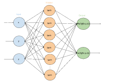
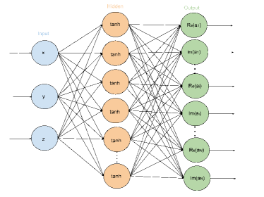
Figure 1: Architectures of the networks used in this work. They both consist of an input layer which gets the coordinates of the position, a non-linear hidden layer, and an output layer which in the first case (left-hand side) provides the real and imaginary part of the probability amplitude, or wave function, and, in the second case(right-hand side) provides the complex coefficients of the series (3).

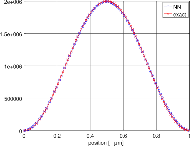
Figure 2: Comparison between the exact solution - (red) cross curve - and the neural network based approach - (blue) circle curve - for the one-dimensional particle in a box problem. Although this is a seminal work, good agreement can already be observed between the numerical and exact probability densities.

5 Numerical Validation

We now present a series of validation tests to show that the method suggested in this paper, although in a preliminary shape, is already in good agreement with the theory. Specifically, these tests consist in finding the ground state of systems made of a single or two-electrons, and compare it with exact or numerically available solutions. The systems taken into account are: one or more electrons 1) in a closed box, 2) inside a finite potential well, and 3) in the presence of a single potential barrier. The numerical details and results are presented in the rest of this section.

An interesting (heuristic) point to keep in mind is that, in all experiments presented in this section, the CMA-ES genetic algorithm has never ended in a local extremum. It has always converged to the ground state of any system that has been approached in this seminal work. Although more investigation is still needed, it represents an initial encouraging sign that it might be utilized in more complex situations. Moreover, all experiments described in this section have been approached by networks with only $16$ hidden units and, yet, they were able to provide the correct answer. To the author, this is a clear indication that this approach might actually be able to reduce the complexity of the Hilbert space.

Particle in a box. The particle in a box model, also known as the infinite potential well, describes a free particle in a finite domain surrounded by two infinite barriers. This problem is one of the very few in quantum mechanics which exact (or analytical) solution is known. Due to its simplicity, this situation represents a good initial benchmark test to validate our approach. The potential energy in this model reads (for simplicity we hereby refer to the one-dimensional case, its generalization to higher dimensions being trivial):

$$V(x)=0,\forall x\in D,$$

where $D$ is a finite spatial domain represented by an interval $[0,L]$. It is possible to show that, in this case, the exact solution of the eigenproblem (1) reads:

$$\psi_{n}(x)=\sqrt{\frac{2}{L}}\sin{(k_{n}x)},$$ (8)

with $k_{n}=\frac{n\pi}{L}$, and

$$E_{n}=\frac{n^{2}\pi^{2}\hbar^{2}}{2mL^{2}},$$ (9)

where $m=9.10938356\times 10^{-31}$ Kg is the mass of the particle (i.e. a free electron). The ground state is, obviously, represented by the case $n=1$.

Below, we report the results of applying the approach discussed in this work along with a comparison with the exact solution. A good agreement can be observed (see Fig. 2) for a domain with $L=1\mu$m. The exact ground state energy can be computed by means of formula (9) and, in this particular case, is equal to $3.7603\times 10^{-7}$ eV. The energy found by our method is equal to $3.7254\times 10^{-7}$ eV, in good agreement with the theory.

A similar test is then performed in a two dimensional space as well (with dimensions $1\mu$m $\times 1\mu$m) and Fig. 3 shows the ground state wave function obtained. One can clearly observe that the expected symmetry of the ground state is respected. The energy found is equal to $7.40031\times 10^{-7}$ eV which is in good agreement with the theoretical value of $7.52061\times 10^{-7}$ eV. Finally, the same test is performed in a three dimensional space with dimensions $1\mu$m $\times 1\mu$m $\times 1\mu$m. The ground state energy is, in this case, expected to be equal to $1.12809\times 10^{-6}$ eV while we obtain a value equal to $1.11548\times 10^{-6}$ eV, again, in good agreement with the theory. Fig. 4 shows the cuts of the three-dimensional ground state on the planes $x=\frac{L_{x}}{2}$, $y=\frac{L_{y}}{2}$ and $z=\frac{L_{z}}{2}$. A very good symmetry structure can be observed.

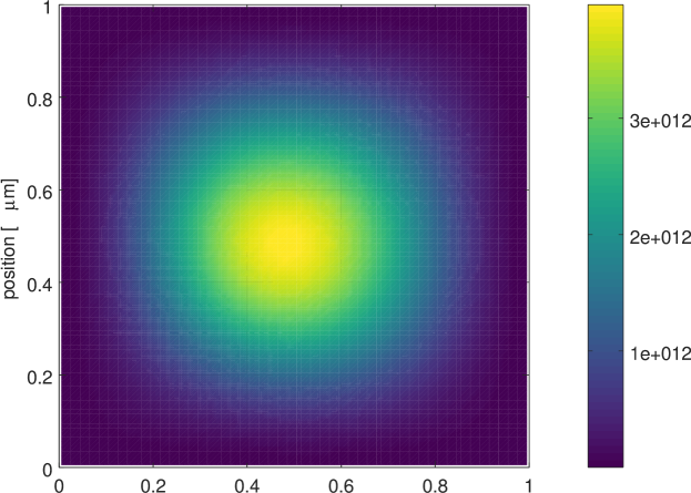
Figure 3: Ground state of a two-dimensional particle in a box found by means of the neural network based approach. One can clearly observe how the expected symmetries of the ground state are respected by this method.

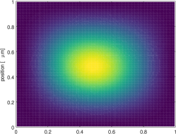
Figure 4: Cut of the three-dimensional ground state for a particle in a box computed by means of a feedforward neural network. The cuts are performed on the planes $x=\frac{L_{x}}{2}$ (left), $y=\frac{L_{y}}{2}$ (middle) and $z=\frac{L_{z}}{2}$ (right) respectively. The symmetry is very well respected on every plane.

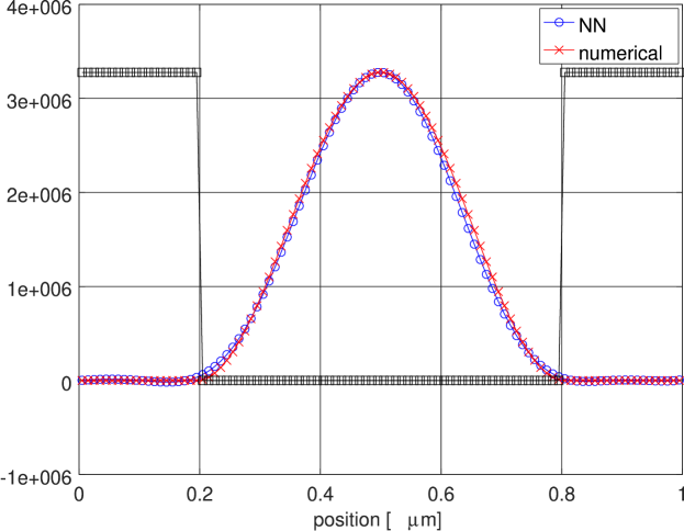
Figure 5: Comparison between a numerically computed solution - (red) cross curve - and the suggested neural network based approach - (blue) circle curve - for the one-dimensional particle in a finite potential well - (black) square curve. A good agreement can be observed.

Finite potential well. The finite potential well is a typical problem of quantum mechanics which can be seen as a generalization of the particle in a box problem. It consists of two barriers placed at the right-hand and left-hand sides of the spatial domain. In such context, if the total energy of the particle is smaller than the energy of the barriers then it cannot be found outside of the box. The results obtained by exploiting a neural network representation of the quantum state are compared to a deterministic eigensolver [6] implemented in the LAPACK library [7], and reported in Fig. 5. The computed numerical value for the energy is equal $3.2363\times 10^{-6}$ eV while the value found by the network approach is equal to $3.2872\times 10^{-6}$ eV. It is clear that a good agreement is reached between two very different approaches.

Single step barrier. In quantum mechanics, the single step potential barrier is a standard problem which illustrates the phenomena of quantum tunneling and reflection. In practice, it consists of solving the time-independent Schrödinger equation (1) in the presence of a potential which reads:

$$V(x)=V_{0},\forall x\in[a,b],$$

and $0$ elsewhere for some value $V_{0}\neq 0$ and $0\leq a<b\leq L$. In particular, for the results presented here, we used $a=\frac{L}{2}$, $b=L$ and $V_{0}=-0.1$ eV. The same domain length as the previous test is utilized. The comparison between the numerically computed solution and the one based on our approach can be seen in Fig. 6. The agreement remains satisfying. In fact, the peaks are found in the same position, and the shape of the two wave functions is practically the same, although some differences between the two solutions can be observed. This could be due to the very different nature of the two methods, being one essentially stochastic and the other deterministic (further investigations are required). In any case, this initial agreement remains promising. Energy-wise, the value found by the standard eigensolver is equal to $1.4450\times 10^{-6}$ eV while the one found with our neural network approach is equal to $1.5872\times 10^{-6}$ eV, another indication that the two methods are in acceptable agreement.

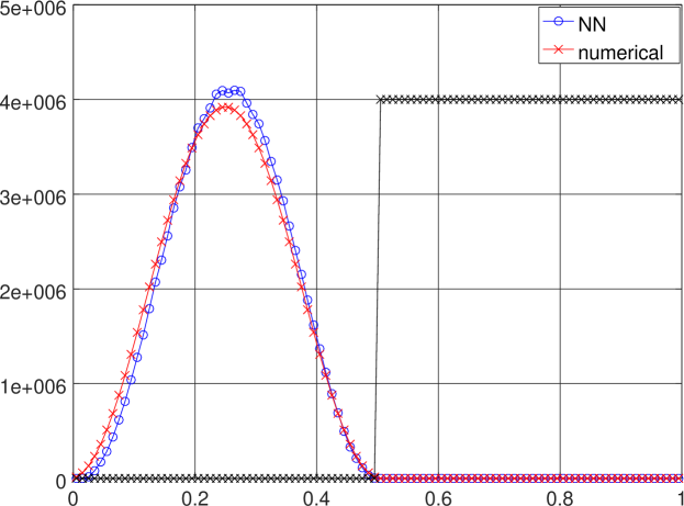
Figure 6: Comparison between the exact solution - (red) cross curve - and the neural network based approach - (blue) circle curve - for the one-dimensional single potential barrier problem. Some differences are noticeable between the numerical and exact probability densities.

Non-interacting particles. An important validation test is represented by the simulation of a quantum system made of $N$ non-interacting electrons. In fact, although it involves a very particular situation, it is one of the few many-body systems which exact solution is known and which can be simply written as the product of single-electron wave functions (Hartree products). In more mathematical details, such a system is characterized by an Hamiltonian which reads:

$$\hat{H}(x_{1},\dots,x_{n})=\sum_{i=1}^{n}\hat{h}_{i}=\sum_{i=1}^{n}[-\frac{\hbar^{2}\partial}{2m_{i}\partial x_{i}}-qV(x_{i})],$$ (10)

where $\hat{h}_{i}$ is an operator acting on the $i$-th particle only, $m_{i}$ is its mass and $q$, as usual, its charge. The exact solution for this problem is well known and can be written in the shape of an Hartree product. The Hartree product is a many-body wave function, given as a combination of wave functions of the individual particles. It assumes that the particles are independent and, therefore, is unsymmetrized. Mathematically, a two-body Hartree product reads:

$$\psi(x_{1},x_{2})=\psi_{1}(x_{1})\psi_{2}(x_{2}),$$

where $\psi_{1}=\psi_{1}(x_{1})$ and $\psi_{2}=\psi_{2}(x_{2})$ are the solutions of the problem

$$\hat{h}_{i}\psi_{i}(x)=\epsilon_{i}\psi_{i}(x).$$

Finally, it can be proven that the total energy of the problem is equal to the sum $\epsilon_{1}+\epsilon_{2}$. This provides a simple way to check the validity of the energy found by the method presented in this work. Moreover, the probability density $n=n(x_{1},x_{2})$ in the configuration space reads:

$$n(x_{1},x_{2}) = \psi^{*}(x_{1},x_{2})\psi(x_{1},x_{2})$$

$$= \psi^{*}_{1}(x_{1})\psi^{*}_{2}(x_{2})\psi_{1}(x_{1})\psi_{2}(x_{2})$$

$$= \psi^{*}_{1}(x_{1})\psi_{1}(x_{1})\psi^{*}_{2}(x_{2})\psi_{2}(x_{2})$$

$$= n_{1}(x_{1})n_{2}(x_{2})$$

which clearly highlights the fact that the two-body density $n=n(x_{1},x_{2})$ is equal to the product of the two one-body densities $n_{1}=n_{1}(x_{1})$ and $n_{2}=n_{2}(x_{2})$. This provides a simple way to check the validity of the wave functions found by our approach.

In this validation test, the spatial domain is now equal to $[0,1.0]$ nm and the theoretical expected energy is equal to the sum of the energies of the single particles, i.e. $0.7520$ eV. The value found with our approach is equal to $0.7537$ eV in excellent agreement with the theory. Fig. 7. We then performed a second numerical experiment still involving two non-interacting particles, one feeling no potential and the other feeling a step potential barrier in the domain $[0,1.0]\mu$m. In this situation, the energy is expected to be lower than $3.7603\times 10^{-7}+1.5041\times 10^{-6}=1.8801\times 10^{-6}$ eV (which corresponds to the energy of a particle confined to the domain length $1.0\mu$m and $0.5\mu$m respectively). Our approach finds a value equal to $1.8603\times 10^{-6}$ eV. Fig. 8 shows the squared magnitude of the computed two-body wave functions defined over the configuration space where one electron feels a step potential barrier and the are does not, and vice-versa. Clearly, the shape of the function corresponds to the one expected. A final test is presented in Fig. 9 showing the probability density for two electrons both feeling the presence of a step potential barrier. The shape of the wave function is, again, the one expected. The energy expected in such system is equal to $2\times 1.5041\times 10^{-6}=3.0082\times 10^{-6}$ eV while the value found with by our approach is equal to $3.2741\times 10^{-6}$ eV, in good agreement with what expected.

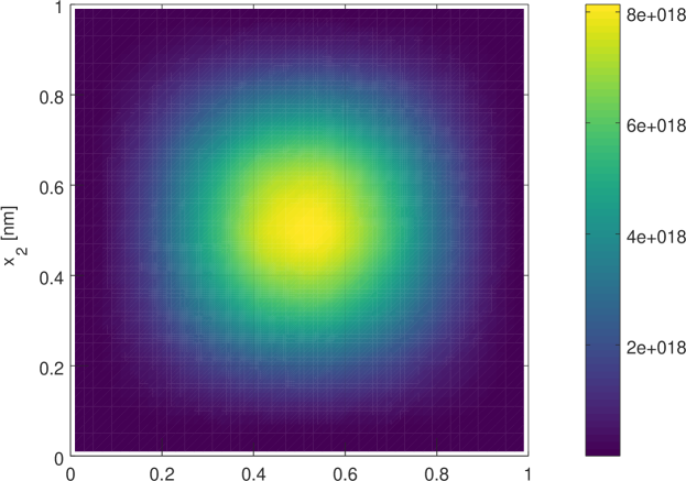
Figure 7: Solution of the 2-body particle-in-a-box problem in the two-dimensional configuration space. A very good symmetry can be observed, in good agreement with the theoretical solution.

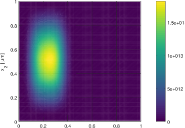
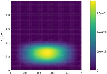
Figure 8: Two solutions of the 2-body problem in the two-dimensional configuration space corresponding to a particle which feels a step barrier and one which does not feel any potential. A very good symmetry can be observed, in good agreement with the theoretical solution.

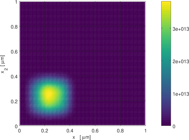
Figure 9: Two solutions of the 2-body problem in the two-dimensional configuration space corresponding to two non-interacting particles in the presence of a step barrier.

Interacting particles. This final validation test represents an important step since it involves exchange effects happening in quantum systems of Fermions. In this context, the Hamiltonian of such systems cannot be expressed as in (10) since they contain an extra term modeling the interaction between particles and which, for the case of electrons, reads:

$$V(x_{1},x_{2})=\frac{q^{2}}{4\pi\epsilon_{0}}\frac{1}{|x_{1}-x_{2}|},$$

and where the constant $\epsilon_{0}$ is the permittivity of vacuum. One should note that in every numerical experiments performed in the context of interacting particles, one expects the total energy of the system to be always bigger than the one involving non-interacting particles, due to the fact that interacting particles are strongly confined not only by the dimensions of the box but also by the Coulombic potential created by the other particles in such system. This is clearly observed from the results obtained by the approach suggested in this work.

The tests consist of finding the ground state of two interacting particles in an empty box first (i.e. two interacting particles in a box), and, then, in the presence of a step potential barrier. The energies found in both cases are $3$ orders of magnitude bigger than their corresponding non-interacting counterparts (i.e. $1.7619\times 10^{-3}$ eV and $4.6467\times 10^{-3}$ eV respectively). The probability density functions for these tests are shown in Fig. 10 (left-hand side is the empty box case, right-hand side corresponds to particles in the presence of a step potential barrier) where the confinement of the electrons is clearly visible (as expected).

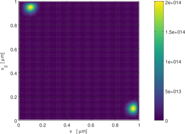
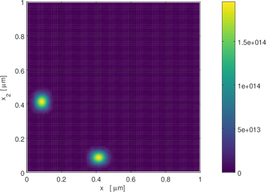
Figure 10: Probability density functions of two interacting Fermions in a empty box (left-hand side) and in the presence of a step potential barrier (right-hand side).

6 Conclusions and Future Works

In this paper, a new method to represent the state of a quantum system, based on the universal representation theorem has been suggested. The method is similar, in its tenets, to the one discussed in [1] but applies to systems beyond spinglasses and exploits feedforward neural networks rather than Boltzmann machines. Several validation tests, involving interacting and non-interacting electrons have been presented which hold the promise of more complex simulations. Many directions still need to be investigated though. For instance, nothing has been said about the non-linear activation functions of the hidden layer and it would be of high interest to see what the effects of such non-linearities (ReLU, etc.) would be on the accuracy of the ground state. The same question could be asked for the depth and width of the network (in this work we have been using single-hidden layer neural networks only). In the same way, the plethora of sampling methods available should be explored to clarify if any further advantage can be obtained. These will be the subject of next future works.

Acknowledgments. The author would like to thank G. Marceau Caron and S. Blackburn for their very fruitful and valuable conversations. A special thanks goes to M. Anti for her loving support and encouragement.

References

- [1] G. Carleo, M. Troyer, Solving the Quantum Many-body Problem with Artificial Neural Networks, Science 355, pp. 602–606, (2017).
- [2] G. Carleo, Y. Nomura, M. Imada, Constructing Exact Representations of Quantum Many-body Systems with Deep Neural Networks, Nature Communications 9, 5322, (2018).
- [3] A.N. Kolmogorov, On the Representation of Continuous Functions of Several Variables by Superposition of Continuous Functions of one Variable and Addition, Doklady Akademii. Nauk USSR, 114, pp. 679-681, (1957).
- [4] G. Cybenko, Approximations by Superpositions of Sigmoidal Functions, Mathematics of Control, Signals, and Systems, 2(4), pp. 303–314, (1989).
- [5] K. Hornik, Approximation Capabilities of Multilayer Feedforward Networks, Neural Networks, 4(2), pp. 251–257, (1991).
- [6] J. Demmel, Computing Small Singular Values of Bidiagonal Matrices with Guaranteed High Relative Accuracy, Forgotten Books, (2018).
- [7] E. Anderson, Z. Bai, C. Bischof, S. Blackford, J. Demmel, J. Dongarra, J. Du Croz, A. Greenbaum, S. Hammarling, A. McKenney, D. Sorensen, LAPACK Users Guide, Society for Industrial and Applied Mathematics, (1999).
- [8] E. Schrödinger, Quantisierung als Eigenwertproblem, Ann. Phys. 385, pp. 437–490, (1926).
- [9] L.V. Keldysh, Zh. Eksp. Teor. Fiz., Sov. Phys. JETP 20, (1965).
- [10] R.P. Feynman, Space–time Approach to Non-relativistic Quantum Mechanics, Rev. Modern Phys. 20, p. 367, (1948).
- [11] E. Wigner, On the Quantum Correction for Thermodynamic Equilibrium, Physical Review 40, no. 5, 749, (1932).
- [12] J.M. Sellier, A Signed Particle Formulation of Non-Relativistic Quantum Mechanics, Journal of Computational Physics 297, pp. 254-265, (2015).
- [13] C.M. Bishop, Neural Networks for Pattern Recognition, Oxford University Press, (1995).
- [14] I. Goodfellow, Y. Bengio, A. Courville, Deep Learning, The MIT Press, (2016).
- [15] N. Hansen, The CMA Evolution Strategy: a Comparing Review, Towards a New Evolutionary Computation. Studies in Fuzziness and Soft Computing, vol 192, Springer, (2006).