A Matrix-Less Method to Approximate the Spectrum and the Spectral Function of Toeplitz Matrices with Real Eigenvalues

Abstract

It is known that the generating function $f$ of a sequence of Toeplitz matrices $\{T_{n}(f)\}_{n}$ may not describe the asymptotic distribution of the eigenvalues of $T_{n}(f)$ if $f$ is not real. In this paper, we assume as a working hypothesis that, if the eigenvalues of $T_{n}(f)$ are real for all $n$, then they admit an asymptotic expansion of the same type as considered in previous works [13, 1, 12, 10], where the first function $g$ appearing in this expansion is real and describes the asymptotic distribution of the eigenvalues of $T_{n}(f)$. After validating this working hypothesis through a number of numerical experiments, drawing inspiration from [12], we propose a matrix-less algorithm in order to approximate the eigenvalue distribution function $g$. The proposed algorithm is tested on a wide range of numerical examples; in some cases, we are even able to find the analytical expression of $g$. Future research directions are outlined at the end of the paper.

1 Introduction

Given a function $f\in L^{1}([-\pi,\pi])$, the $n\times n$ Toeplitz matrix generated by $f$ is defined as

$$T_{n}(f)=\left[\begin{array}[]{ccccccccc}\hat{f}_{0}&\hat{f}_{-1}&\cdots&\hat{f}_{n-1}\vphantom{\vdots}\\ \hat{f}_{1}&\ddots&\ddots&\vdots\\ \vdots&\ddots&\ddots&\hat{f}_{-1}\\ \hat{f}_{n-1}&\cdots&\hat{f}_{1}&\hat{f}_{0}\vphantom{\vdots}\\ \\[-6.00006pt] \end{array}\right],$$ (6)

where the numbers $\hat{f}_{k}$ are the Fourier coefficients of $f$, that is,

$$\hat{f}_{k}=\frac{1}{2\pi}\int_{-\pi}^{\pi}f(\theta)e^{-\mathbf{i}k\theta}\mathrm{d}\theta,\qquad f(\theta)=\sum_{k=-\infty}^{\infty}\hat{f}_{k}e^{\mathbf{i}k\theta}.$$ (7)

It is known that the generating function $f$, also known as the symbol of $\{T_{n}(f)\}_{n}$, describes the asymptotic distribution of the singular values of $T_{n}(f)$; if $f$ is real or if $f\in L^{\infty}([-\pi,\pi])$ and its essential range has empty interior and does not disconnect the complex plane, then $f$ also describes the asymptotic distribution of the eigenvalues of $f$; see [8, 15, 20] for details and [15, Section 3.1] for the notion of asymptotic singular value and eigenvalue distribution of a sequence of matrices. We will write $\{T_{n}(f)\}_{n}\sim_{\sigma}f$ to indicate that $\{T_{n}(f)\}_{n}$ has an asymptotic singular value distribution described by $f$ and $\{T_{n}(f)\}_{n}\sim_{\lambda}f$ to indicate that $\{T_{n}(f)\}_{n}$ has an asymptotic eigenvalue distribution described by $f$. The cases of interest in this paper are those in which $\{T_{n}(f)\}_{n}\not\sim_{\lambda}f$ and the eigenvalues of $T_{n}(f)$ are real for all $n$. We believe that in these cases there exist a real function $g$ such that $\{T_{n}(f)\}_{n}\sim_{\lambda}g$ and the eigenvalues of $T_{n}(f)$ admit an asymptotic expansion of the same type as considered in previous works [13, 1, 12, 10]. We therefore formulate the following working hypothesis.

Working Hypothesis.

Suppose that the eigenvalues of $T_{n}(f)$ are real for all $n$. Then, for every integer $\alpha\geq 0$, every $n$ and every $j=1,\ldots,n$, the following asymptotic expansion holds:

$$\lambda_{j}(T_{n}(f)) =g(\theta_{j,n})+\sum_{k=1}^{\alpha}c_{k}(\theta_{j,n})h^{k}+E_{j,n,\alpha},$$

$$=\sum_{k=0}^{\alpha}c_{k}(\theta_{j,n})h^{k}+E_{j,n,\alpha},$$ (8)

where:

• the eigenvalues of $T_{n}(f)$ are arranged in non-decreasing order, $\lambda_{1}(T_{n}(f))\leq\ldots\leq\lambda_{n}(T_{n}(f))$;

• $\{g\coloneqq c_{0},c_{1},c_{2},c_{3},\ldots\}$ is a sequence of functions from $(0,\pi)$ to $\mathbb{R}$ which depends only on $f$;

• $h=\frac{1}{n+1}$ and $\theta_{j,n}=\frac{j\pi}{n+1}=j\pi h$;

• $E_{j,n,\alpha}=O(h^{\alpha+1})$ is the remainder (the error), which satisfies the inequality $|E_{j,n,\alpha}|\leq C_{\alpha}h^{\alpha+1}$ for some constant $C_{\alpha}$ depending only on $\alpha,f$.

Remark 1.

In the working hypothesis, we arrange the eigenvalues of $T_{n}(f)$ in non-decreasing order, however, using a non-increasing order would result in another function $g$. The case where the eigenvalues of $T_{n}(f)$ can be described by a complex-valued or non-monotone function $g$ is out of the scope of this article and warrants further research.

2 Motivation and illustrative examples

In this section we present four examples in support of our working hypothesis. We also discuss the fact that standard double precision eigenvalue solvers (such as LAPACK, eig in Matlab, and eigvals in Julia) fail to give accurate eigenvalues of certain matrices $T_{n}(f)$; see, e.g., [3, 21]. High-precision computations, by using packages such as GenericLinearAlgebra.jl [16] in Julia can compute the true eigenvalues, but they are very expensive from the computational point of view. Therefore, approximating $g$ on the grid $\theta_{j,n}$ and using matrix-less methods [12] to compute the spectrum of $T_{n}(f)$ can be computationally very advantageous. Also, the presented approaches can be a valuable tool for the analysis of the spectra of non-normal Toplitz matrices having real eigenvalues.

Here is a short description of the four examples we are going to consider. In what follows, we denote by $\xi_{j,n}$ a “perfect” sampling grid, typically not equispaced, such that $\lambda_{j}(T_{n}(f))=g(\xi_{j,n})$ for $j=1,\ldots,n$; such grids are discussed in [9].

• Example 1: $T_{n}(f)$ is non-symmetric tridiagonal, $g$ is known, and the eigenvalues $\lambda_{j}(T_{n}(f))=g(\theta_{j,n})$ are known explicitly;

• Example 2: $T_{n}(f)$ is symmetric pentadiagonal, $g=f$, and the eigenvalues $\lambda_{j}(T_{n}(f))=g(\xi_{j,n})$ are not known explicitly;

• Example 3: $T_{n}(f)$ is non-symmetric, $g$ is known, and the eigenvalues $\lambda_{j}(T_{n}(f))=g(\xi_{j,n})$ are not known explicitly;

• Example 4: $T_{n}(f)$ is non-symmetric, $g$ is not known, and the eigenvalues $\lambda_{j}(T_{n}(f))=g(\xi_{j,n})$ are not known explicitly.

Example 1.

Consider the symbol

$$f(\theta) =\hat{f}_{1}e^{\mathbf{i}\theta}+\hat{f}_{0}+\hat{f}_{-1}e^{-\mathbf{i}\theta}.$$ (9)

The matrix $T_{n}(f)$ is tridiagonal, and there exist a function

$$g(\theta)=\hat{f}_{0}+2\sqrt{\hat{f}_{1}}\sqrt{\hat{f}_{-1}}\cos(\theta),$$ (10)

such that $T_{n}(f)\sim T_{n}(g)$, that is, they are similar and hence have the same eigenvalues. The eigenvalues are given explicitly by

$$\lambda_{j}(T_{n}(f))=g(\theta_{j,n}),$$ (11)

where $\theta_{j,n}$ is defined in the working hypothesis. Now, choose the Fourier coefficients $\hat{f}_{1}=-1$, $\hat{f}_{0}=2$, and $\hat{f}_{-1}=-2$. In this case, we have

$$f(\theta) =-e^{\mathbf{i}\theta}+2-2e^{-\mathbf{i}\theta},$$

$$g(\theta) =2-2\sqrt{2}\cos(\theta),$$ (12)

and the spectrum of $T_{n}(f)$ is real, even though the symbol $f$ is complex-valued. The Toeplitz matrices generated by $f$ and $g$ are given by

$$T_{n}(f)=\left[\begin{array}[]{rrrrr}2&-2\\ -1&2&-2\\ &\ddots&\ddots&\ddots\\ &&\ddots&\ddots&-2\\ &&&-1&2\end{array}\right],\quad T_{n}(g)=\left[\begin{array}[]{rrrrr}2&-\sqrt{2}\\ -\sqrt{2}&2&-\sqrt{2}\\ &\ddots&\ddots&\ddots\\ &&\ddots&\ddots&-\sqrt{2}\\ &&&-\sqrt{2}&2\end{array}\right],$$ (23)

We also note that $T_{n}(g)$ is a symmetrized version of $T_{n}(f)$, in the sense that there exists a decomposition $T_{n}(g)=DT_{n}(f)D^{-1}$ where $D$ is a diagonal matrix with elements $(D)_{i,i}=\gamma^{i-1}$, and $\gamma=\sqrt{\hat{f}_{-1}}/\sqrt{\hat{f}_{1}}$; see [17].

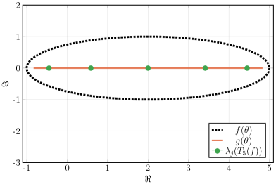
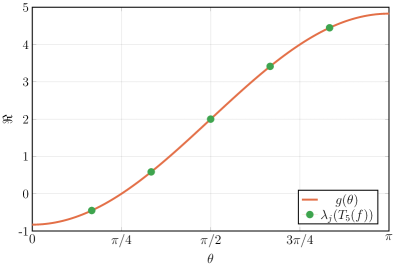
Figure 1: [Example 1: Symbol $f(\theta)=-e^{\mathbf{i}\theta}+2-2e^{-\mathbf{i}\theta}$] Left: Representations of $f(\theta)$ (dashed black line), and $g(\theta)=2-2\sqrt{2}\cos(\theta)$ (red line), and $\lambda_{j}(T_{n}(f))=\lambda_{j}(T_{n}(g))$ for $n=5$ (green dots). Right: Representations of $g$ and $\lambda_{j}(T_{5}(f))=\lambda_{j}(T_{5}(g))=g(\theta_{j,n})$.

In the left panel of Figure 1 we represent the function $f$ (dashed black line), and $g$ (red line), and the eigenvalues $\lambda_{j}(T_{n}(f))=\lambda_{j}(T_{n}(g))$ (green dots) for $n=5$. In the right panel of Figure 1 we show the function $g$ (red line) on the interval $[0,\pi]$ only (since it is even on $[-\pi,\pi]$) and the eigenvalues $\lambda_{j}(T_{5}(f))=\lambda_{j}(T_{5}(g))=g(\theta_{j,5})$ (green dots).

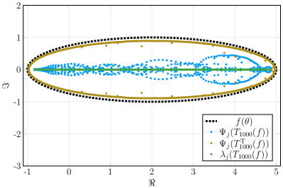
Figure 2: [Example 1: Symbol $f(\theta)=-e^{\mathbf{i}\theta}+2-2e^{-\mathbf{i}\theta}$] Symbol $f(\theta)$ (dashed black line), the numerically computed spectra (using a standard double precision eigenvalue solver) $\Psi_{j}(T_{1000}(f))$ (blue dots), $\Psi_{j}(T_{1000}^{\mathrm{T}}(f))$ (beige dots), and the analytical spectrum $\lambda_{j}(T_{1000}(f))=g(\theta_{j,1000})$ (green dots).

In Figure 2 we present the numerically computed spectra $\Psi_{j}(T_{n}(f))$ (blue dots) and $\Psi_{j}(T_{n}^{\mathrm{T}}(f))$ (beige dots), for $n=1000$, using a standard double precision eigenvalue solver. The analytical spectrum, defined by (11) and (12) is also shown (green dots). These numerically computed eigenvalues $\Psi_{j}(A_{n})$ are related to the pseudospectrum, discussed for example in [21, 3, 18].

Example 2.

In this example we consider the symbol

$$f(\theta) =(2-2\cos(\theta))^{2}=6-8\cos(\theta)+2\cos(\theta)$$

which generates a Toeplitz matrix $T_{n}(f)$ associated with the second order finite difference approximation of the bi-Laplacian,

$$T_{n}(f)=\left[\begin{array}[]{rrrrrrrrrrr}6&-4&1\vphantom{\ddots}\\ -4&6&-4&1\vphantom{\ddots}\\ 1&-4&6&-4&1\vphantom{\ddots}\\ &\ddots&\ddots&\ddots&\ddots&\ddots\\ &&\ddots&\ddots&\ddots&\ddots&1\\ &&&\ddots&\ddots&\ddots&-4\\ &&&&1&-4&6\vphantom{\ddots}\end{array}\right].$$ (31)

The matrices $T_{n}(f)$ are all Hermitian and sothey have a real spectrum. Moreover, we have $f(\theta)=g(\theta)$, and $\{T_{n}(f)\}_{n}\sim_{\sigma,\lambda}f$. In Figure 3 we represent the symbol $g=f$ and the eigenvalues of $T_{n}(f)$ for $n=5$. The “perfect” sampling grid $\xi_{j,n}$ such that $\lambda_{j}(T_{n}(f))=g(\xi_{j,n})$ is not equispaced, but can in this case be obtained by either computing $\xi_{j}=2\sin^{-1}\left((\lambda_{j}(T_{n}(f)))^{1/4}/2\right)$ (since $f(\theta)=16\sin^{4}(\theta/2)$), finding the roots in $(0,\pi)$ of $g(\theta)-\lambda_{j}(T_{n}(f))$, or using the expansion described in [9] for large $n$.

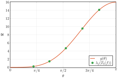
Figure 3: [Example 2: Symbol $f(\theta)=6-8\cos(\theta)+2\cos(2\theta)$] Symbol $g(\theta)=f(\theta)$ and $\lambda_{j}(T_{5}(f))=g(\xi_{j,5})$.

Example 3.

In this example we consider the following symbol

$$f(\theta) =e^{\mathbf{i}\theta}-4+6e^{-\mathbf{i}\theta}-4e^{-2\mathbf{i}\theta}+e^{-3\mathbf{i}\theta}$$

$$=e^{-\mathbf{i}\theta}\left(6-8\cos(\theta)+2\cos(\theta)\right).$$

The Toeplitz matrix $T_{n}(f)$ is a shifted version of the matrix considered in Example 2 (that is, the matrix associated with the second order finite difference approximation of the bi-Laplacian), and it is given by

$$T_{n}(f)=\left[\begin{array}[]{rrrrrrrrrrr}-4&6&-4&1\vphantom{\ddots}\\ 1&-4&6&-4&1\vphantom{\ddots}\\ &\ddots&\ddots&\ddots&\ddots&\ddots\\ &&\ddots&\ddots&\ddots&\ddots&1\\ &&&\ddots&\ddots&\ddots&-4\\ &&&&\ddots&\ddots&6\\ &&&&&1&-4\vphantom{\ddots}\end{array}\right].$$ (39)

We note that

$$f(\theta) =e^{-\mathbf{i}\theta}\left(2-2\cos(\theta)\right)^{2}$$

$$=e^{-3\mathbf{i}\theta}\left(1-e^{\mathbf{i}\theta}\right)^{4},$$

which is equivalent to (41) in [19, Example 3.] with $z=e^{\mathbf{i}\theta}$, $a=-1,r=3$, and $s=1$. Hence by (43) in the same article we have that

$$g(\theta)=-\frac{\sin^{4}(\theta)}{\sin(\theta/4)\sin^{3}(3\theta/4)},$$ (40)

and the matrix $T_{n}(g)$ would be full with $\lambda_{j}(T_{n}(f))\approx\lambda_{j}(T_{n}(g))\in(-\frac{(r+s)^{r+s}}{r^{r}s^{s}},0)=(-\frac{256}{27},0)$ for all $j$.

In the left panel of Figure 4 we represent the functions $f$ (dashed black line), $g$ (red line) and the eigenvalues $\lambda_{j}(T_{n}(f))$ (green dots) for $n=5$. In the right panel of Figure 4 we show the function $g$ (red line) on the interval $[0,\pi]$ only (since it is even on $[-\pi,\pi]$) and the eigenvalues $\lambda_{j}(T_{5}(f))=g(\xi_{j,5})$ (green dots).

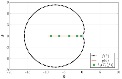
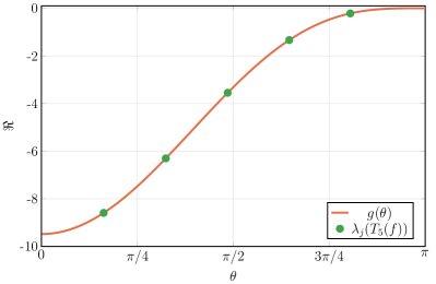
Figure 4: [Example 3: Symbol $f(\theta)=e^{-\mathbf{i}\theta}\left(6-8\cos(\theta)+2\cos(\theta)\right)$] Left: Representations of $f(\theta)$ (dashed black line), $g(\theta)=-\sin^{4}(\theta)/(\sin(\theta/4)\sin^{3}(3\theta/4))$ (red line), and $\lambda_{j}(T_{n}(f))$ for $n=5$ (green dots). Right: Representation of $g$ and $\lambda_{j}(T_{5}(f))=g(\xi_{j,5})$.

In Figure 5 we present the numerically computed spectra $\Psi_{j}(T_{n}(f))$ (blue dots) and $\Psi_{j}(T_{n}^{\mathrm{T}}(f))$ (beige dots), for $n=1000$, using a standard double precision eigenvalue solver. The approximations of the true eigenvalues $\lambda_{j}(T_{1000}(f))=g{\xi_{j,1000}}$ (green dots) are also shown, computed with 128 bit precision.

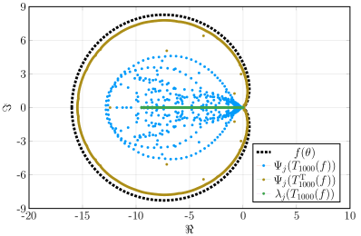
Figure 5: [Example 3: Symbol $f(\theta)=e^{-\mathbf{i}\theta}\left(6-8\cos(\theta)+2\cos(\theta)\right)$] Symbol $f(\theta)$ (dashed black line), the numerically computed spectra (using a standard double precision eigenvalue solver) $\Psi_{j}(T_{1000}(f))$ (blue dots), $\Psi_{j}(T_{1000}^{\mathrm{T}}(f))$ (beige dots), and approximated spectrum $\lambda_{j}(T_{1000}(f))=g(\xi_{j,1000})$ (green dots).

Example 4.

In this example we consider a symbol $f$ where the explicit formula for $g$ is not known explicitly. Let

$$f(\theta)=e^{3\mathbf{i}\theta}-e^{2\mathbf{i}\theta}+7e^{\mathbf{i}\theta}+9e^{-1\mathbf{i}\theta}-2e^{-2\mathbf{i}\theta}+2e^{-3\mathbf{i}\theta}-e^{-4\mathbf{i}\theta},$$

which generates the matrix

$$T_{n}(f)=\left[\begin{array}[]{rrrrrrrrrrrrrrr}0&9&-2&2&-1\vphantom{\ddots}\\ 7&0&9&-2&2&-1\vphantom{\ddots}\\ -1&7&0&9&-2&2&-1\vphantom{\ddots}\\ 1&-1&7&0&9&-2&2&-1\vphantom{\ddots}\\ &\ddots&\ddots&\ddots&\ddots&\ddots&\ddots&\ddots&\ddots\\ &&\ddots&\ddots&\ddots&\ddots&\ddots&\ddots&\ddots&-1\\ &&&\ddots&\ddots&\ddots&\ddots&\ddots&\ddots&2\\ &&&&\ddots&\ddots&\ddots&\ddots&\ddots&-2\\ &&&&&\ddots&\ddots&\ddots&\ddots&9\\ &&&&&&1&-1&\hphantom{-}7&0\vphantom{\ddots}\\ \end{array}\right].$$ (51)

From [19, Example 4.] we have strong indications that approximately $\lambda_{j}(T_{n}(f))\in[-22.09,14.96]$ for all $j$.

In the left panel of Figure 6 we represent the symbol $f$ (dashed black line) and the eigenvalues $\lambda_{1000}(T_{n}(f))$, computed with a 256 bit eigenvalue solver (dashed red line) since $g$ is not known. The eigenvalues $\lambda_{j}(T_{n}(f))$ (green dots) for $n=5$ are also shown. In the right panel of Figure 6 show again the eigenvalues $\lambda_{1000}(T_{n}(f))$ arranged in non-decreasing order (dashed red line) since $g$ is not known on the interval $[0,\pi]$, since it is even on $[-\pi,\pi]$. Also the eigenvalues $\lambda_{j}(T_{5}(f))=g(\xi_{j,5})$ (green dots) are represented. The “perfect” grid $\xi_{j,n}$ is computed using data from Example 8. Numerically we have $\lambda_{j}(T_{1000}(f))\in[-22.0912,14.9641]$ in agreement with [19].

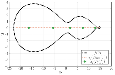
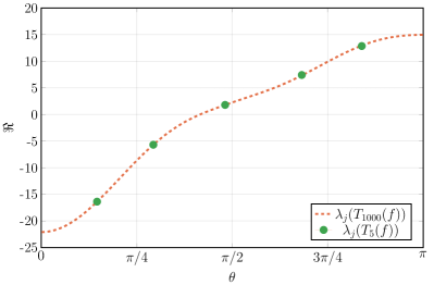
Figure 6: [Example 4: Symbol $f(\theta)=e^{3\mathbf{i}\theta}-e^{2\mathbf{i}\theta}+7e^{\mathbf{i}\theta}+9e^{-1\mathbf{i}\theta}-2e^{-2\mathbf{i}\theta}+2e^{-3\mathbf{i}\theta}-e^{-4\mathbf{i}\theta}$] Left: Symbol $f(\theta)$ (dashed black line) and $\lambda_{j}(T_{1000}(f))$ (dashed red line) since $g(\theta)$ is unknown, and $\lambda_{j}(T_{n}(f))$ for $n=5$ (green dots). Right: Eigenvalues $\lambda_{j}(T_{1000}(f))$ ordered in non-decreasing order and $\lambda_{j}(T_{5}(f))=g(\xi_{j,5})$.

In Figure 7 we present the numerically computed spectra $\Psi_{j}(T_{n}(f))$ (blue dots) and $\Psi_{j}(T_{n}^{\mathrm{T}}(f))$ (beige dots), for $n=1000$, using a standard double precision eigenvalue solver. The true eigenvalues $\lambda_{j}(T_{1000}(f))=g(\xi_{j,1000})$ (green dots) are approximated using a 256 bit precision computation.

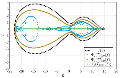
Figure 7: [Example 4: Symbol $f(\theta)=e^{3\mathbf{i}\theta}-e^{2\mathbf{i}\theta}+7e^{\mathbf{i}\theta}+9e^{-1\mathbf{i}\theta}-2e^{-2\mathbf{i}\theta}+2e^{-3\mathbf{i}\theta}-e^{-4\mathbf{i}\theta}$] Symbol $f(\theta)$ (dashed black line), the numerically computed spectra $\Psi_{j}(T_{1000}(f))$ (blue dots), $\Psi_{j}(T_{1000}^{\mathrm{T}}(f))$ (beige dots), and $\lambda_{j}(T_{1000}(f))=g(\xi_{j,n})$ (green dots).

3 Describing the real-valued eigenvalue distribution

Assuming that $g$ is a real cosine trigonometric (RCTP) symbol associated with a symbol $f$ as in the working hypothesis, we introduce in Section 3.1 a new matrix-less method to accurately compute the expansion functions $c_{k},k=0,\ldots,\alpha$, where we recall that $c_{0}=g$. Subsequently, in Section 3.2 we present procedures to obtain an approximation or even the analytical expression of $g$.

3.1 Approximating the expansion functions $c_{k}$ in grid points $\theta_{j,n_{0}}$

An asymptotic expansion of the eigenvalue errors $E_{j,n,0}\coloneqq E_{j,n}$, when sampling the symbol $f$ with the grid $\theta_{j,n}$ defined in the working hypothesis, under certain assumptions on $f$ implying that $g=f$, was discussed in a series of papers [5, 6, 7]; such expansion can be deduced from

$$\lambda_{j}(T_{n}(f))=f(\theta_{j,n})+\underbrace{\sum_{k=1}^{\alpha}c_{k}(\theta_{j,n})h^{k}+E_{j,n,\alpha}}_{E_{j,n}},$$ (52)

where $\theta_{j,n}$, $h$, and $E_{j,n,\alpha}$ are defined in the working hypothesis.

An algorithm was proposed in [13] to approximate the functions $c_{k}(\theta)$, which was subsequently extended to other types of Toeplitz-like matrices $A_{n}$ possessing an asymptotic expansion such as (52); see [1, 11, 10, 12]. We call this type of methods matrix-less, since they do not need to construct the large matrix $A_{n}$ to approximate its eigenvalues; indeed, they approximate the functions $c_{k}(\theta)$ from $\alpha$ small matrices $A_{n_{1}},\ldots,A_{n_{\alpha}}$ and then they use this approximations to compute the approximate spectrum of $A_{n}$ through the formula

$$\lambda_{j}(A_{n})\approx\tilde{\lambda}_{j}(A_{n})=f(\theta_{j,n})+\sum_{k=1}^{\alpha}\tilde{c}_{k}(\theta_{j,n})h^{k}.$$ (53)

Assuming that the eigenvalues of $T_{n}(f)$ admit an asymptotic expansion in terms of an unknwn function $g$ instead of $f$, as in our working hypothesis, we can use a slight modification of Algorithm 1 in [14, Section 2.1] in order to find approximations of both $g$ and the eigenvalues of $T_{n}(f)$ through the following formula, analogous to (53):

$$\lambda_{j}(T_{n}(f))\approx\tilde{\lambda}_{j}(T_{n}(f)) =\sum_{k=0}^{\alpha}\tilde{c}_{k}(\theta_{j,n})h^{k}$$

$$=\tilde{g}(\theta_{j,n})+\sum_{k=1}^{\alpha}\tilde{c}_{k}(\theta_{j,n})h^{k},$$ (54)

where the approximation $\tilde{g}(\theta)\coloneqq\tilde{c}_{0}(\theta)$ of $g(\theta)\coloneqq c_{0}(\theta)$ is obtained from $\alpha+1$ small matrices $T_{n_{0}}(f),\ldots,T_{n_{\alpha}}(f)$ as mentioned above.

Here follows an implementation in Julia of the algorithm that computes the approximations $\tilde{c}_{k}(\theta)$ for $k=0,\ldots,\alpha$; the algorithm is written for clarity and not performance. All computations in this article are made with Julia 1.1.0 [4], using Float64 and BigFloat data types, and the GenericLinearAlgebra.jl package [16].

Algorithm 1.

Approximate expansion functions $c_{k}(\theta)$ for $k=0,\ldots,\alpha$ on the grid $\theta_{j,n_{0}}$.

⬇

using LinearAlgebra, GenericLinearAlgebra

setprecision(BigFloat,128)

# Example: computeC(100, 4, BigFloat[2, -1], BigFloat[2, -2])

function computeC(n0 :: Integer, # Number of grid points in grid theta_{j,n0}

alpha :: Integer, # Number of c_k to approximate, k=0,...,alpha

vc :: Array{T,1}, # First column of T_n(f)

vr :: Array{T,1}, # First row of T_n(f)

revorder :: Bool=false # Reverse ordering of eigenvalues of T_n(f)

) where T

j0 = 1:n0

E = zeros(T,alpha+1,n0)

hs = zeros(T,alpha+1)

for kk = 1:alpha+1

nk = 2^(kk-1)*(n0+1)-1

jk = 2^(kk-1)*j0

hs[kk] = convert(T,1)/(nk+1)

Tnk = Toeplitz(nk,vc,vr)

eTnk = eigvals(Tnk)

if !isreal(eTnk)

error("Spectrum not real. Decrease n0 or alpha, or use BigFloat with higher precision.")

end

eTnk = sort(real.(eTnk),rev=revorder)

E[kk,:] = eTnk[jk]

end

V = zeros(T,alpha+1,alpha+1)

for ii = 1:alpha+1, jj = 1:alpha+1

V[ii,jj] = hs[ii]^(jj-1)

end

return C=V\E # Output: Matrix C, size (alpha+1,n0), with approximations c_k(theta_{j,n0})

end

# Example: Toeplitz(100, Float64[2, -1], Float64[2, -2])

function Toeplitz(n :: Integer, # Order of Toeplitz matrix T_n(f)

vc :: Array{T,1}, # First column of T_n(f)

vr :: Array{T,1} # First row of T_n(f)

) where T

Tn = zeros(T,n,n)

for ii = 1:length(vc)

Tn = Tn + diagm(-ii+1 => vc[ii]*ones(T,n-ii+1))

end

for jj = 2:length(vr)

Tn = Tn + diagm( jj-1 => vr[jj]*ones(T,n-jj+1))

end

return Tn # Output: Toeplitz matrix of order n, defined by vectors vc and vr

end

Using the output $\tilde{c}_{k}(\theta_{j,n_{0}})$, we can employ the interpolation–extrapolation technique described in [12] to efficiently compute very accurate approximations of $\tilde{c}_{k}(\theta)$ and, through (54), the eigenvalues of $T_{n}(f)$ for an arbitrarily large order $n$. In the next section, we focus on the use of the approximations $\tilde{c}_{0}=\tilde{g}$ to describe $g$.

3.2 Constructing a function $g$ from approximations $\tilde{g}(\theta_{j,n_{0}})=\tilde{c}_{0}(\theta_{j,n_{0}})$

We here assume, for the sake of simplicity, that the sought function $g$ is real and even, so that it admits a cosine Fourier series of the form

$$g(\theta)=\hat{g}_{0}+2\sum_{k=1}^{\infty}\hat{g}_{k}\cos(k\theta),\qquad\hat{g}_{k}\in\mathbb{R}.$$ (55)

As we shall see, if $g$ is a real cosine trigonometric polynomial (RCTP), that is, a function of the form

$$g(\theta)=\hat{g}_{0}+2\sum_{k=1}^{m}\hat{g}_{k}\cos(k\theta),\qquad\hat{g}_{k}\in\mathbb{R},$$ (56)

then we will be able to recover the exact expression of $g$ (see Examples 5 and 6); otherwise, we will get a truncated representation of the Fourier expansion of $g$ in (55) (see Examples 7 and 8). More specifically, what we do is the following: we consider the approximations $\tilde{c}_{0}(\theta_{j,n_{0}})$ provided by Algorithm 1 and we approximate the first $n_{0}$ Fourier coefficients $\hat{g}_{0},\ldots,\hat{g}_{n_{0}}$ with the numbers $\tilde{\hat{g}}_{0},\ldots,\tilde{\hat{g}}_{n_{0}}$ obtained by solving the linear system

$$\tilde{\hat{g}}_{0}+2\sum_{k=1}^{n_{0}}\tilde{\hat{g}}_{k}\cos(k\theta_{j,n_{0}})=\tilde{c}_{0}(\theta_{j,n_{0}}),\qquad j=1,\ldots,n_{0}.$$ (57)

Algorithm 2.

Compute approximations $\tilde{\hat{g}}_{k}$ of the Fourier coefficients $\hat{g}_{k}$ of $g(\theta)$.

⬇

# Example: computeghattilde(C[1,:])

function computeghattilde(c0 :: Array{T,1}) where T # Array of approximations c_0(theta_{j,n0})

n0 = length(c0)

t = LinRange(convert(T,pi)/(n0+1),n0*convert(T,pi)/(n0+1),n0)

G = zeros(T,n0,n0)

G[:,1] = ones(T,n0)

for jj = 2:n0

G[:,jj] = 2*cos.((jj-1)*t)

end

return ghattilde = G\c0 # Output: Coefficients ghattilde in (13)

end

4 Numerical examples

We now employ the proposed Algorithms 1 and 2 on a the symbols $f$ discussed in Examples 1–4 to highlight the applicability of the approach, in the respective Examples 5–8.

• Example 5: Only $\tilde{c}_{0}$ is non-zero, since $\theta_{j,n}$ gives exact eigenvalues, and the function $g$ is constructed.

• Example 6: Symbol $f=c_{0}$, and $c_{k},k=1,\ldots,4$, are recovered accurately, and the function $g=f$ is constructed.

• Example 7: Symbol $g=c_{0}$, and $c_{k},k=1,\ldots,4$, are recovered accurately, and a truncated RCTP representation of of $g$ is constructed.

• Example 8: Symbol $g=c_{0}$, and $c_{k},k=1,\ldots,4$, are constructed, and a truncated RCTP representation of of $g$ is constructed.

Example 5.

We return to the non-symmetric symbol $f(\theta)=-e^{\mathbf{i}\theta}+2-2e^{-\mathbf{i}\theta}$ of Example 1, and first use the proposed Algorithm 1. Note that care has to be taken when using for example standard Matlab eig command, since already for $n=160$ the returned eigenvalues are complex-valued (and wrong). In such a circumstance a choice of $n_{0}$ and $\alpha$ needs to be such that $n_{\alpha}=2^{\alpha}(n_{0}+1)-1<160$. However, we here also use an arbitrary precision solver, GenericLinearAlgebra.jl in Julia, so we can increase precision such that theoretically any combination of $n_{0}$ and $\alpha$ can be chosen. The performance however decreases fast as we increase the computational precision, showing the need for the current proposed algorithms.

In Figure 8 we present the computation of $\tilde{c}_{k}(\theta_{j,n_{0}})$, for $n_{0}=31$, and different precision and $\alpha$. In the left panel we show the approximated expansion functions $\tilde{c}_{k}$, $k=0,\ldots,\alpha$, where $\alpha=4$, and 128 bit precision computation. As is seen, the only non-zero $\tilde{c}_{k}$ is $\tilde{c}_{0}$, which is expected since the exact eigenvalues are given by $g(\theta_{j,n_{0}})=c_{0}(\theta_{j,n})$. In the right panel of Figure 8 we show the absolute error in the approximation of $c_{0}(\theta_{j,n_{0}})$ for double precision computation, with $\alpha=2$, and 128 bit computation, with $\alpha=4$.

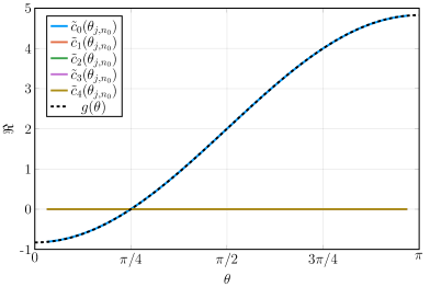
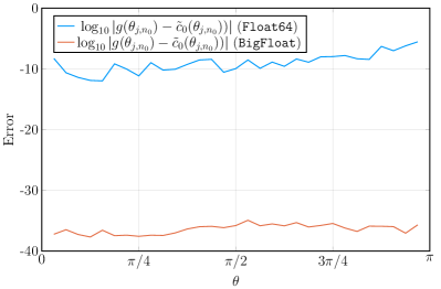
Figure 8: [Example 5: Symbol $f(\theta)=-e^{\mathbf{i}\theta}+2-2e^{-\mathbf{i}\theta}$] The computed $\tilde{c}_{k}(\theta_{j,n_{0}})$, $k=0,\ldots\alpha$, $n_{0}=31$ using Algorithm 1. Left: Computation using 128 bit precision with $\alpha=4$. Only $\tilde{c}_{0}(\theta_{j,n_{0}})=\tilde{g}(\theta_{j,n_{0}})$ are non-zero. Right: The absolute errors of $\tilde{c}_{0}(\theta_{j,n})$ compared with $g(\theta_{j,n})$ for double precision computation, with $\alpha=2$, and 128 bit precision, with $\alpha=4$.

Now we employ Algorithm 2 to compute the Fourier coefficients of $g$. For illustrative purposes we only show a subset of the system (57). If we choose $n_{0}=2^{\beta}-1$, we have three grid points $\theta_{j_{\beta},n_{0}}$ equal to $\pi/4,\pi/2$ and $3\pi/4$, corresponding to indices $j_{\beta}=2^{\beta-2}\{1,2,3\}$. We then have

$$\left[\begin{array}[]{ccc}1&\sqrt{2}&0\\ 1&0&-1\\ 1&-\sqrt{2}&0\end{array}\right]\left[\begin{array}[]{c}\tilde{\hat{g}}_{0}\\ \tilde{\hat{g}}_{1}\\ \tilde{\hat{g}}_{2}\end{array}\right]\approx\left[\begin{array}[]{c}\tilde{c}_{0}(\pi/4)\\ \tilde{c}_{0}(\pi/2)\\ \tilde{c}_{0}(3\pi/4)\end{array}\right].$$ (67)

We construct the following system with $\tilde{c}_{0}$ computed with $n_{0}=31$ (that is, $\beta=5$ and $\alpha=2$ above) using double precision, and subsequently we compute $[\tilde{\hat{g}}_{0},\tilde{\hat{g}}_{1},\tilde{\hat{g}}_{2}]^{\mathrm{T}}$,

$$\left[\begin{array}[]{ccc}1&\sqrt{2}&0\\ 1&0&-1\\ 1&-\sqrt{2}&0\end{array}\right]\left[\begin{array}[]{c}\tilde{\hat{g}}_{0}\\ \tilde{\hat{g}}_{1}\\ \tilde{\hat{g}}_{2}\end{array}\right]\approx\left[\begin{array}[]{r}0.000000000006924\\ 1.999999999889880\\ 3.999999989588136\end{array}\right],\quad\left[\begin{array}[]{c}\tilde{\hat{g}}_{0}\\ \tilde{\hat{g}}_{1}\\ \tilde{\hat{g}}_{2}\end{array}\right]\approx\left[\begin{array}[]{r}1.999999994797530\\ -1.414213558689498\\ -0.000000005092350\end{array}\right].$$ (83)

We conclude from this computation that $g(\theta)=\hat{g}_{0}+2\hat{g}_{1}\cos(\theta)+2\hat{g}_{2}\cos(2\theta)=2-2\sqrt{2}\cos(\theta)$, which is the already known analytical expression; see (11) and (12). Note also that, in this simple example, the vector containing $\tilde{c}_{0}(\theta_{j_{\beta},n_{0}})$ can be assumed to be equal to $[0,2,4]^{\mathrm{T}}$, which would yield the exact solution (to machine precision). Using the full system (57) in Algorithm 2 yields the same result. If we now would approximate the monotonically non-increasing $g$ (instead of the non-decreasing) in Algorithm 1 the vector containing $\tilde{c}(\theta_{j_{\beta},n_{0}})$ would be $[4,2,0]^{\mathrm{T}}$ and would yield the symbol $g(\theta)=2+2\sqrt{2}\cos(\theta)$. Obviously, the eigenvalues of $T_{n}(g)$ are the same for both versions of $g$.

Example 6.

We here return to the symmetric symbol $f(\theta)=(2-2\cos(\theta))^{2}=6-8\cos(\theta)+2\cos(2\theta)$, as in Example 2. Since we know $\{T_{n}(f)\}_{n}\sim_{\sigma,\lambda}f=g$, employing Algorithm 1 will return as $\tilde{c}_{0}$ an approximation of $g$, and as $\tilde{c}_{k}$, $k>0$ the expansion functions previously obtained and studied in [2, 14].

In Figure 9 we show in the left panel the approximated expansion functions $\tilde{c}_{k}(\theta_{j,n_{0}})$ for $k=0,\ldots,\alpha$, computed using $n_{0}=100$, $\alpha=4$. Computations are made with double precision. In the right panel of Figure 9 we show the absolute error of the approximation of $g$, that is, $\log_{10}|g(\theta_{j,n_{0}})-\tilde{c}_{0}(\theta_{j,n_{0}})|$.

The erratic behavior of $\tilde{c}_{4}(\theta)$ close to $\theta=0$ in the left panel, and the increased error close to to $\theta=0$ in the right panel are due to the fact that the symbol $f$ violates the so-called simple-loop conditions, discussed in [2, 14].

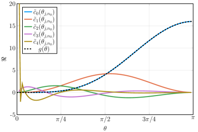
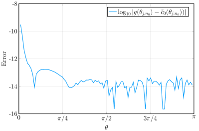
Figure 9: [Example 6: Symbol $f(\theta)=6-8\cos(\theta)+2\cos(2\theta)$] Left: The approximated expansion functions $\tilde{c}_{k}(\theta_{j,n_{0}}),k=0,\ldots,\alpha$ for $n_{0}=100$ and $\alpha=4$. Right: The absolute error $\log_{10}|g(\theta_{j,n_{1}})-\tilde{c}_{0}(\theta_{j,n_{1}})|$.

Using Algorithm 2 we compute approximations of the Fourier coefficients of the mononically increasing $g$ to be $\tilde{\hat{g}}_{0}=6,\tilde{\hat{g}}_{1}=-4$, $\tilde{\hat{g}}_{2}=1$, and $\tilde{\hat{g}}_{k}=0$ for $k>2$. We thus recover the true symbol $g(\theta)=f(\theta)=\hat{g}_{0}+2\hat{g}_{1}\cos(\theta)+2\hat{g}_{2}\cos(2\theta).$ If Algorithm 1 was used to compute $\tilde{c}_{k}$ for the monotonically decreasing $g$ instead, the computed Fourier coefficients would be $\tilde{\hat{g}}_{0}=6,\tilde{\hat{g}}_{1}=4$, and $\tilde{\hat{g}}_{2}=1$. In fact, for $g(\theta)=6\pm 8\cos(\theta)+2\cos(2\theta)$ we have the same eigenvalues for $T_{n}(f)$ and $T_{n}(g)$.

Example 7.

In this example we continue the investigation of $f(\theta)=e^{-\mathbf{i}\theta}(6-8\cos(\theta)+2\cos(2\theta))$ from Example 3. In Figure 10 we show in the left panel the approximated expansion functions $\tilde{c}_{k}(\theta_{j,n_{0}})$ for $n_{0}=100$ and $\alpha=4$. Computations are made with 256 bit precision and the approximation $\tilde{c}_{0}(\theta_{j,n_{0}})$ overlaps well with $g$, defined in (40). Note the erratic behavior of $\tilde{c}_{4}$ close to $\theta=\pi$. In the right panel of Figure 10 we show the absolute values of the first one houndred approximated Fourier coefficients $\tilde{\hat{g}}_{k}$, given by Algorithm 2. In Table 1 we present the first ten true Fourier coefficients, $\hat{g}_{k}$, computed with $g$ defined in (40) and (7), and the approximations $\tilde{\hat{g}}_{k}$ from Algorithm 2. Since $g$ is not an RCTP we can not recover the original simple expression of the symbol (40), but we can anyway obtain an approximated expression of $g$ through our Algorithm 2.

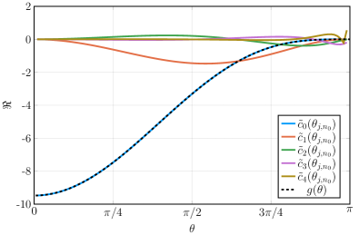
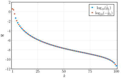
Figure 10: [Example 7: Symbol $f(\theta)=e^{-\mathbf{i}\theta}(6-8\cos(\theta)+2\cos(2\theta))$] Left: The approximated expansion functions $\tilde{c}_{k}(\theta_{j,n_{0}}),k=0,\ldots,\alpha$ for $n_{0}=100$ and $\alpha=4$. The approximation $\tilde{c}_{0}(\theta_{j,n_{0}})$ overlaps well with $g(\theta)=-\sin^{4}(\theta)/(\sin(\theta/4)\sin^{3}(3\theta/4))$. Note the erratic behaviour of $\tilde{c}_{4}$ close to $\theta=\pi$. Right: The absolute value of the approximated first one houndred Fourier coefficients, $\log_{10}|\tilde{\hat{g}}_{k}|$.

Table 1: [Example 7: Symbol $f(\theta)=e^{-\mathbf{i}\theta}(6-8\cos(\theta)+2\cos(2\theta))$] First ten true ($\hat{g}_{k}$) and computed ($\tilde{\hat{g}}_{k}$) Fourier coefficients of $g$. Approximations computed using $n_{0}=100$ and $\alpha=4$, and 256 bit precision.

$k$	$\hat{g}_{k}$	$\tilde{\hat{g}}_{k}$
0	$-4.000000000000000$	$-3.999999999436239$
1	$-2.423215805461417$	$-2.423215806024005$
2	$-0.354481702999765$	$-0.354481702436023$
3	$0.046583829909932$	$0.046583829347381$
4	$-0.013008232443064$	$-0.013008231879376$
5	$0.004790313798591$	$0.004790313236114$
6	$-0.002068441503570$	$-0.002068440939976$
7	$0.000995276400689$	$0.000995275838326$
8	$-0.000518988396995$	$-0.000518987833535$
9	$0.000288215823752$	$0.000288215261541$

Example 8.

Finally, we return to the non-symmetric symbol discussed in Example 4, that is, $f(\theta)=e^{3\mathbf{i}\theta}-e^{2\mathbf{i}\theta}+7e^{\mathbf{i}\theta}+9e^{-1\mathbf{i}\theta}-2e^{-2\mathbf{i}\theta}+2e^{-3\mathbf{i}\theta}-e^{-4\mathbf{i}\theta}$. Again, we employ Algorithms 1 and 2 to study the symbols $f$ and $g$. In the left panel of Figure 11 we present the approximated expansion functions in the working hypothesis, for $n_{0}=100$ and $\alpha=4$. Computations are made with 512 bit precision. The blue line, $\tilde{c}_{0}(\theta_{j,n_{0}})$ corresponds to the approximation of the unknown symbol $g$. Recall the curve of $\lambda_{j}(T_{1000}(f))$ in the right panel of Figure 6, which in principal matches the current $\tilde{c}_{0}$. Note how all $\tilde{c}_{k}$, for $k>0$, are zero in apparently the same point $\theta_{0}\in[\frac{55\pi}{101},\frac{56\pi}{101}]$. In the right panel of Figure 11 we see the first one houndred approximated Fourier coefficients of $g$, by using Algorithm 2. In Table 2 is presented the first ten approximated Fourier coefficients, $\tilde{\hat{g}}_{k}$.

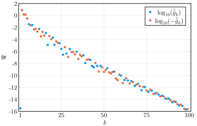
Figure 11: [Example 8: Symbol $f(\theta)=e^{3\mathbf{i}\theta}-e^{2\mathbf{i}\theta}+7e^{\mathbf{i}\theta}+9e^{-1\mathbf{i}\theta}-2e^{-2\mathbf{i}\theta}+2e^{-3\mathbf{i}\theta}-e^{-4\mathbf{i}\theta}$] Left: The approximated expansion functions $\tilde{c}_{k}(\theta_{j,n_{0}}),k=0,\ldots,\alpha$ for $n_{0}=100$ and $\alpha=4$. The approximation $\tilde{c}_{0}(\theta_{j,n_{0}})$ correspond well with $\lambda_{j}(T_{1000}(f))$ in the right panel of Figure 6 (since $g$ is unknown). Right: The absolute value of the approximated first one houndred Fourier coefficients, $\log_{10}|\tilde{\hat{g}}_{k}|$.

Table 2: [Example 8: Symbol $f(\theta)=e^{3\mathbf{i}\theta}-e^{2\mathbf{i}\theta}+7e^{\mathbf{i}\theta}+9e^{-1\mathbf{i}\theta}-2e^{-2\mathbf{i}\theta}+2e^{-3\mathbf{i}\theta}-e^{-4\mathbf{i}\theta}$] First ten computed ($\tilde{\hat{g}}_{k}$) Fourier coefficients of the unknown $g$. Approximations computed using $n_{0}=100$ and $\alpha=4$, and 512 bit precision.

k	$\tilde{\hat{g}}_{k}$
0	$-0.000000000000003$
1	$-7.931536795875190$
2	$-1.429849731406187$
3	$-1.393034471115375$
4	$-0.321121280053002$
5	$0.035288447846840$
6	$-0.023038821632295$
7	$0.026692519463291$
8	$-0.004916206049977$
9	$-0.006047350374789$

5 Conclusions

The working hypothesis in this article concerns the existence of an asymptotic expansion, such that there exists of a function $g$ describing the eigenvalue distribution of the Toeplitz matrices $T_{n}(f)$ generated by a symbol $f$. We have shown numerically that we can recover an approximation of the function $g$. This is done by a matrix-less method described in Algorithm 1, which in principle can be modified so as to work without any information on $f$ or the way in which the eigenvalues of the smaller versions of $T_{n}(f)$ are computed. Algorithm 1 can also be used to fast and accurately compute the eigenvalues of $T_{n}(f)$ for an arbitrarily large order $n$, as highlighted in (54). However, in this article we have focused only on using the obtained approximation of $g$ to find an approximation of its truncated Fourier series; and if $g$ is an RCTP, we have shown that it we are able to recover the original function $g$ analytically. These approaches can be a valuable tool for the exploration of the spectrum of Toeplitz and Toeplitz-like matrices previously not easily understood, because of high computational cost. For future research we propose the extension to complex-valued functions $g$ of the results presented herein, and also the study of matrices more general than $T_{n}(f)$.

6 Acknowledgments

The author would like to thank Carlo Garoni and Stefano Serra-Capizzano for valuable insights and suggestions during the preparation of this work. The author is financed by Athens University of Economics and Business.

References

- [1] F. Ahmad, E. S. Al-Aidarous, D. A. Alrehaili, S.-E. Ekström, I. Furci, and S. Serra-Capizzano, Are the eigenvalues of preconditioned banded symmetric Toeplitz matrices known in almost closed form?, Numerical Algorithms, 78 (2017), pp. 867–893.
- [2] M. Barrera, A. Böttcher, S. M. Grudsky, and E. A. Maximenko, Eigenvalues of even very nice Toeplitz matrices can be unexpectedly erratic, in The Diversity and Beauty of Applied Operator Theory, Springer International Publishing, 2018, pp. 51–77.
- [3] R. M. Beam and R. F. Warming, The Asymptotic Spectra of Banded Toeplitz and Quasi-Toeplitz Matrices, SIAM Journal on Scientific Computing, 14 (1993), pp. 971–1006.
- [4] J. Bezanson, A. Edelman, S. Karpinski, and V. B. Shah, Julia: A Fresh Approach to Numerical Computing, SIAM Review, 59 (2017), pp. 65–98.
- [5] J. M. Bogoya, A. Böttcher, S. M. Grudsky, and E. A. Maximenko, Eigenvalues of Hermitian Toeplitz matrices with smooth simple-loop symbols, Journal of Mathematical Analysis and Applications, 422 (2015), pp. 1308–1334.
- [6] J. M. Bogoya, S. M. Grudsky, and E. A. Maximenko, Eigenvalues of Hermitian Toeplitz Matrices Generated by Simple-loop Symbols with Relaxed Smoothness, in Large Truncated Toeplitz Matrices, Toeplitz Operators, and Related Topics, Springer International Publishing, 2017, pp. 179–212.
- [7] A. Böttcher, S. M. Grudsky, and E. A. Maxsimenko, Inside the eigenvalues of certain Hermitian Toeplitz band matrices, Journal of Computational and Applied Mathematics, 233 (2010), pp. 2245–2264.
- [8] A. Böttcher and B. Silbermann, Introduction to Large Truncated Toeplitz Matrices, Springer New York, 1999.
- [9] S.-E. Ekström, Approximating the Perfect Sampling Grids for Computing the Eigenvalues of Toeplitz-like Matrices Using the Spectral Symbol, 2019. arXiv:1901.06917 (submitted).
- [10] S.-E. Ekström, I. Furci, C. Garoni, C. Manni, S. Serra-Capizzano, and H. Speleers, Are the eigenvalues of the B-spline isogeometric analysis approximation of known in almost closed form?, Numerical Linear Algebra with Applications, 25 (2018), p. e2198.
- [11] S.-E. Ekström, I. Furci, and S. Serra-Capizzano, Exact formulae and matrix-less eigensolvers for block banded symmetric Toeplitz matrices, BIT Numerical Mathematics, 58 (2018), pp. 937–968.
- [12] S.-E. Ekström and C. Garoni, A matrix-less and parallel interpolation–extrapolation algorithm for computing the eigenvalues of preconditioned banded symmetric Toeplitz matrices, Numerical Algorithms, (2018). https://doi.org/10.1007/s11075-018-0508-0 (in press).
- [13] S.-E. Ekström, C. Garoni, and S. Serra-Capizzano, Are the Eigenvalues of Banded Symmetric Toeplitz Matrices Known in Almost Closed Form?, Experimental Mathematics, 27 (2017), pp. 478–487.
- [14] S.-E. Ekström, Matrix-Less Methods for Computing Eigenvalues of Large Structured Matrices, PhD thesis, Uppsala University, Uppsala: Acta Universitatis Upsaliensis, 2018.
- [15] C. Garoni and S. Serra-Capizzano, Generalized Locally Toeplitz Sequences: Theory and Applications (Volume 1), Springer International Publishing, 2017.
- [16] A. Noack, GenericLinearAlgebra.jl. https://github.com/JuliaLinearAlgebra/GenericLinearAlgebra.jl.
- [17] S. V. Parter and J. Youngs, The symmetrization of matrices by diagonal matrices, Journal of Mathematical Analysis and Applications, 4 (1962), pp. 102–110.
- [18] L. Reichel and L. N. Trefethen, Eigenvalues and pseudo-eigenvalues of Toeplitz matrices, Linear Algebra and its Applications, 162-164 (1992), pp. 153–185.
- [19] B. Shapiro and F. Štampach, Non-Self-Adjoint Toeplitz Matrices Whose Principal Submatrices Have Real Spectrum, Constructive Approximation, (2017). https://doi.org/10.1007/s00365-017-9408-0 (in press).
- [20] P. Tilli, Some results on complex Toeplitz eigenvalues, Journal of Mathematical Analysis and Applications, 239 (1999), pp. 390–401.
- [21] L. N. Trefethen and M. Embree, Spectra and pseudospectra: the behavior of nonnormal matrices and operators, Princeton University Press, Princeton, N.J, 2005.