Refined Meshless Local Strong Form solution of
Cauchy-Navier equation on an irregular domain

Abstract

This paper considers a numerical solution of a linear elasticity problem, namely the Cauchy-Navier equation, using a strong form method based on a local Weighted Least Squares (WLS) approximation. The main advantage of the employed numerical approach, also referred to as a Meshless Local Strong Form method, is its generality in terms of approximation setup and positions of computational nodes. In this paper, flexibility regarding the nodal position is demonstrated through two numerical examples, i.e. a drilled cantilever beam, where an irregular domain is treated with a relatively simple nodal positioning algorithm, and a Hertzian contact problem, where again, a relatively simple h-refinement algorithm is used to extensively refine discretization under the contact area. The results are presented in terms of accuracy and convergence rates, using different approximations and refinement setups, namely Gaussian and monomial based approximations, and a comparison of execution time for each block of the solution procedure.

1 Introduction

Linear elasticity problems, governed by the Cauchy-Navier equation, are typically addressed in their weak form with the Finite Elements Method (FEM) [1]. However, the problem has also been addressed in its strong form in the past, e.g. component-wise iterative solution with the Finite Differences Method (FDM) [2] and with the Finite Volumes Method (FVM) [3]. Besides mesh based methods, meshless methods have also been employed for solving solid mechanics problems in strong and weak form [4, 5]. The conceptual difference between meshless methods and mesh based methods is in the treatment of relations between nodes. In the mesh based methods the nodes need to be structured into polygons (mesh) that cover the whole computational domain, while on the other hand, meshless methods fully define relations between nodes through the relative inter nodal positions [6], with an immediate consequence of greater generality of the meshless methods.

Strong form meshless methods can be understood as generalizations of FDM, where instead of predetermined interpolation over a local support, a more general approach with variable support and basis is used to evaluate partial differential operators [7], e.g. collocation using Radial Basis Functions [5, 8] or approximation with monomial basis  [9]. There are many other methods with more or less similar methodology introducing new variants of the strong form meshless principle [10]. On the other hand, weak form meshless methods are generalizations of FEM. Probably the most known method among weak form meshless methods is the Meshless Local Petrov Galerkin Method (MLPG) [11], where for each integration point a local support is used to evaluate field values and weight functions of a Moving Least Squares (MLS) approximation are used as test functions. In last few decades there have been many variants of MLPG introduced to mitigate numerical instabilities and to improve accuracy and convergence rate, etc. [10].

In general, recent developments in meshless community are vivid, ranging from analyses of computer execution on different platforms [6, 12], reducing computational cost by introducing a piecewise approximation [13] to implementation of more complex multi-phase flow [14], and many more.

This paper extends the spectra of published papers with a generalized formulation of a local strong form meshless method, termed Meshless Local Strong Form Method (MLSM) enriched with h-refinement [15] and ability to discretize arbitrary domains [7].

The introduced meshless approach is demonstrated on a solution of a benchmark cantilever beam case [16] and a Hertzian contact problem [17]. The results are presented in terms of displacement and stress plots, comparison against closed form solutions, convergence analyses, and execution time analyses.

The goal of this paper is to demonstrate generality of MLSM that is driven by the fact that all the building blocks of the method depend only on the relative positions between the computational nodes. This is a very useful feature, especially when dealing with problems in multidimensional spaces, complex geometries, and moving boundaries. This feature can be also exploited to write elegant generic code [18].

The rest of the paper is organized as follows: in section 2 the MLSM principle is explained, in section 3 the governing problem is introduced, section 4 is focused on solution procedure, section 5 focuses on discussing the results, and finally, the paper offers some conclusions and guidelines for future work in the last section.

2 MLSM formulation

The core of the spatial discretization used in this paper is a local approximation of a considered field over the overlapping local support domains, i.e. in each node we use approximation over a small local subset of neighbouring $n$ nodes. The trial function $\hat{u}$ is thus introduced as

$$\hat{u}(\vec{p})=\sum_{i=1}^{m}\alpha_{i}b_{i}(\vec{p})=\boldsymbol{b}(\vec{p})^{\mathsf{T}}\boldsymbol{\alpha},$$ (1)

with $m$, $\boldsymbol{\alpha}$, $\boldsymbol{b}$ and $\vec{p}$ standing for the number of basis functions, approximation coefficients, basis functions and the position vector, respectively. In cases when the number of basis functions and the number of nodes in the support domain are the same, $n=m$, the determination of coefficients $\boldsymbol{\alpha}$ simplifies to solving a system of $n$ linear equations, resulting from evaluating equation (1) in each support node and setting it equal to a true value $u(\vec{p}_{j})$, for $j$ from 1 to $n$:

$$u_{j}:=u(\vec{p}_{j})=\boldsymbol{b}(\vec{p}_{j})^{\mathsf{T}}\boldsymbol{\alpha},$$ (2)

where $\vec{p}_{j}$ are positions of support nodes and $u_{j}$ is the actual value of considered field in the support node $\vec{p}_{j}$. The above system can be written in matrix form as

$$\boldsymbol{u}=\boldsymbol{B}\boldsymbol{\alpha},$$ (3)

where $\boldsymbol{B}$ stands for coefficient matrix with elements $B_{ji}=b_{i}(\vec{p}_{j})$. The most known method that uses such an approach is the Local Radial Basis Function Collocation Method (LRBFCM) that has been recently used in various problems [5, 8].

In cases when the number of support nodes is higher than the number of basis functions ($n>m$) a WLS approximation is chosen as a solution of equation (3), which becomes an overdetermined problem. An example of this approach is DAM [9] that was originally formulated to solve fluid flow in porous media. DAM uses six monomials for basis and nine noded support domains to evaluate first and second derivatives of physical fields required to solve the problem at hand, namely the Navier Stokes equation. To determine the approximation coefficients $\boldsymbol{\alpha}$, a norm

$$R^{2}=\sum_{j}^{n}{w(\vec{p}_{j})(u(\vec{p}_{j})-\hat{u}(\vec{p}_{j}))}^{2}=(\boldsymbol{B\alpha}-\boldsymbol{u})^{\mathsf{T}}\boldsymbol{W}^{2}(\boldsymbol{B\alpha}-\boldsymbol{u}),$$ (4)

is minimized, where $\boldsymbol{W}$ is a diagonal matrix with elements $W_{jj}=\sqrt{w(\vec{p}_{j})}$ with

$$w(\vec{p})=\exp\left(-\left(\frac{\|\vec{p}_{0}-\vec{p}\|}{\sigma p_{\text{min}}}\right)^{2}\right),$$ (5)

where $\sigma$ stands for weight shape parameter, $\vec{p}_{0}$ for centre of support domain and $p_{\text{min}}$ for the distance to the nearest support domain node. There are different computational approaches to minimizing (4). The most intuitive and also computationally effective is to simply compute the gradient of $R^{2}$ with respect to $\boldsymbol{\alpha}$ and setting it to zero, resulting in a positive definite system

$$\boldsymbol{B}^{\mathsf{T}}\boldsymbol{W}^{2}\boldsymbol{B}\boldsymbol{\alpha}=\boldsymbol{B}^{\mathsf{T}}\boldsymbol{W}^{2}\boldsymbol{u}.$$ (6)

The problem of this approach is bad conditioning, as the condition number of $\boldsymbol{B}^{\mathsf{T}}\boldsymbol{W}^{2}\boldsymbol{B}$ is the square of the condition number of $\boldsymbol{WB}$, unnecessarily increasing numerical instability. A more stable and more expensive approach is QR decomposition. An even more stable approach is SVD decomposition, which is of course even more expensive. Nevertheless, the solution of equation (6) can be written generally in matrix form as

$$\boldsymbol{\alpha}=(\boldsymbol{W}\boldsymbol{B})^{+}\boldsymbol{W}\boldsymbol{u},$$ (7)

where $\boldsymbol{A}^{+}$ stands for a Moore–Penrose pseudo inverse of matrix $\boldsymbol{A}$. By explicitly inserting equation (7) for $\boldsymbol{\alpha}$ into (1), the equation

$$\hat{u}(\vec{p})=\boldsymbol{b}(\vec{p})^{\mathsf{T}}(\boldsymbol{W}\boldsymbol{B})^{+}\boldsymbol{W}\boldsymbol{u}=\boldsymbol{\chi}(\vec{p})\boldsymbol{u},$$ (8)

is obtained, where $\boldsymbol{\chi}=\boldsymbol{b}(\vec{p})^{\mathsf{T}}(\boldsymbol{W}\boldsymbol{B})^{+}\boldsymbol{W}$ is called a shape function. Now, we can apply a partial differential operator $\mathcal{L}$ to the trial function, and get

$$(\mathcal{L}\hat{u})(\vec{p})=(\mathcal{L}\boldsymbol{\chi})(\vec{p})\boldsymbol{u}.$$ (9)

In this paper we deal with a Cauchy-Navier equation and therefore following shape functions are needed, expressed explicitly as

$$\boldsymbol{\chi}^{\partial x}(\vec{p}) =\frac{\partial\boldsymbol{b}}{\partial x}(\vec{p})^{\mathsf{T}}(\boldsymbol{W}\boldsymbol{B})^{+}\boldsymbol{W},$$ (10)

$$\boldsymbol{\chi}^{\partial y}(\vec{p}) =\frac{\partial\boldsymbol{b}}{\partial y}(\vec{p})^{\mathsf{T}}(\boldsymbol{W}\boldsymbol{B})^{+}\boldsymbol{W},$$ (11)

$$\boldsymbol{\chi}^{\partial x\partial x}(\vec{p}) =\frac{\partial^{2}\boldsymbol{b}}{\partial x^{2}}(\vec{p})^{\mathsf{T}}(\boldsymbol{W}\boldsymbol{B})^{+}\boldsymbol{W},$$ (12)

$$\boldsymbol{\chi}^{\partial x\partial y}(\vec{p}) =\frac{\partial^{2}\boldsymbol{b}}{\partial x\partial y}(\vec{p})^{\mathsf{T}}(\boldsymbol{W}\boldsymbol{B})^{+}\boldsymbol{W},$$ (13)

$$\boldsymbol{\chi}^{\partial y\partial y}(\vec{p}) =\frac{\partial^{2}\boldsymbol{b}}{\partial^{2}y}(\vec{p})^{\mathsf{T}}(\boldsymbol{W}\boldsymbol{B})^{+}\boldsymbol{W}.$$ (14)

The shape functions depend only on the numerical setup, namely nodal distribution, shape parameter, basis and support selection, and can as such be precomputed for a specific computation.

3 Governing problem

The goal in this paper is to numerically determine the stress and displacement distributions in a solid body subjected to the applied external force. To obtain a displacement vector field $\vec{u}$ throughout the domain, a Cauchy-Navier equation is solved, which can expressed concisely in vector form as

$$(\lambda+\mu)\nabla(\nabla\cdot\vec{u})+\mu\nabla^{2}\vec{u}=0,$$ (15)

where $\mu$ and $\lambda$ stand for Lamé constants. In two dimensions we express $\vec{u}=(u,v)$ and the equation reads

$$(\lambda+\mu)\frac{\partial}{\partial x}\left(\frac{\partial u}{\partial x}+\frac{\partial v}{\partial y}\right)+\mu\left(\frac{\partial^{2}u}{\partial x^{2}}+\frac{\partial^{2}u}{\partial y^{2}}\right) =0$$ (16)

$$(\lambda+\mu)\frac{\partial}{\partial y}\left(\frac{\partial u}{\partial x}+\frac{\partial v}{\partial y}\right)+\mu\left(\frac{\partial^{2}v}{\partial x^{2}}+\frac{\partial^{2}v}{\partial y^{2}}\right) =0$$ (17)

Two types of boundary conditions are commonly used when solving these types of problems, namely essential boundary conditions and traction (also called natural) boundary conditions. Essential boundary conditions specify displacements on some portion of the boundary of the domain, i.e. $\vec{u}=\vec{u}_{0}$, while traction boundary conditions specify surface traction $\sigma\vec{n}=\vec{t}_{0}$, where $\vec{n}$ is an outside unit normal to the boundary of the domain and

$$\sigma=\begin{bmatrix}\sigma_{xx}&\sigma_{xy}\\ \sigma_{xy}&\sigma_{yy}\end{bmatrix}$$ (18)

is the stress tensor. In terms of displacement vector $\vec{u}$ the traction boundary conditions read

$${t_{0}}_{1} =\mu n_{2}\frac{\partial u}{\partial y}+\lambda n_{1}\frac{\partial v}{\partial y}+(2\mu+\lambda)n_{1}\frac{\partial u}{\partial x}+\mu n_{2}\frac{\partial v}{\partial x}$$ (19)

$${t_{0}}_{2} =\mu n_{1}\frac{\partial u}{\partial y}+(2\mu+\lambda)n_{2}\frac{\partial v}{\partial y}+\lambda n_{2}\frac{\partial u}{\partial x}+\mu n_{1}\frac{\partial v}{\partial x}$$ (20)

where ${t_{0}}_{i}$ and $n_{i}$ denote the Cartesian components of $\vec{t}_{0}$ and $\vec{n}$.

4 Solution procedure

4.1 Discretization of the problem

The elliptic boundary value problem at hand is discretized into a linear system of $2N$ algebraic equations by approximating the differential operations using MLSM, as described in section 2. A block system of linear equations for two vectors $\boldsymbol{u}$ and $\boldsymbol{v}$ of unknowns representing values $u(\vec{p_{i}})$ and $v(\vec{p_{i}})$, respectively, is constructed. This system is a discrete analogy of PDE (15) and can symbolically be represented as

$$\begin{bmatrix}U1&V1\\ U2&V2\end{bmatrix}\begin{bmatrix}\boldsymbol{u}\\ \boldsymbol{v}\end{bmatrix}=\begin{bmatrix}\boldsymbol{b_{1}}\\ \boldsymbol{b_{2}}\end{bmatrix},$$ (21)

where $\boldsymbol{u}$ and $\boldsymbol{v}$ stand for unknown displacements, $\boldsymbol{b_{1}}$ and $\boldsymbol{b_{2}}$ for values of boundary conditions and blocks $U1,V1,U2,V2$ contain precomputed shape functions (10–14). With $\mathcal{N}(i)$ standing for a list of indices of the chosen $n$ neighbours of a point $\vec{p}_{i}$, as introduced in the beginning of section 2, we can, for all indices $i$ of internal nodes, express

$$\left.\begin{aligned} U1_{i,\mathcal{N}(i)_{j}}&=\left[(\lambda+2\mu)\boldsymbol{\chi}^{\partial x\partial x}(\vec{p}_{i})+\mu\boldsymbol{\chi}^{\partial y\partial y}(\vec{p}_{i})\right]_{j}\\ V1_{i,\mathcal{N}(i)_{j}}&=\left[(\lambda+\mu)\boldsymbol{\chi}^{\partial x\partial y}(\vec{p}_{i})\right]_{j}\\ {\boldsymbol{b}_{1}}_{i}&=0\end{aligned}\right\},$$ (22)

$$\left.\begin{aligned} U2_{i,\mathcal{N}(i)_{j}}&=\left[(\lambda+\mu)\boldsymbol{\chi}^{\partial x\partial y}(\vec{p}_{i})\right]_{j}\\ V2_{i,\mathcal{N}(i)_{j}}&=\left[\mu\boldsymbol{\chi}^{\partial x\partial x}(\vec{p}_{i})+(\lambda+2\mu)\boldsymbol{\chi}^{\partial y\partial y}(\vec{p}_{i})\right]_{j}\\ {\boldsymbol{b}_{2}}_{i}&=0\\ \end{aligned}\right\},$$ (23)

for each $j=1,\ldots,n$. Note that equation (22) represents direct discrete analogue of (16) and, likewise, (23) of (17).

Similarly, for all indices $i$ of boundary nodes with traction boundary conditions we express

$$\left.\begin{aligned} U1_{i,\mathcal{N}(i)_{j}}&=\left[\mu n_{2}\boldsymbol{\chi}^{\partial y}(\vec{p}_{i})+(2\mu+\lambda)n_{1}\boldsymbol{\chi}^{\partial x}(\vec{p}_{i})\right]_{j}\\ V1_{i,\mathcal{N}(i)_{j}}&=\left[\lambda n_{1}\boldsymbol{\chi}^{\partial y}(\vec{p}_{i})+\mu n_{2}\boldsymbol{\chi}^{\partial x}(\vec{p}_{i})\right]_{j}\\ {\boldsymbol{b}_{1}}_{i}&={t_{0}}(\vec{p}_{i})_{1}\end{aligned}\right\},$$ (24)

$$\left.\begin{aligned} U2_{i,\mathcal{N}(i)_{j}}&=\left[\mu n_{1}\boldsymbol{\chi}^{\partial y}(\vec{p}_{i})+\lambda n_{2}\boldsymbol{\chi}^{\partial x}(\vec{p}_{i})\right]_{j}\\ V2_{i,\mathcal{N}(i)_{j}}&=\left[\mu n_{1}\boldsymbol{\chi}^{\partial x}(\vec{p}_{i})+(2\mu+\lambda)n_{2}\boldsymbol{\chi}^{\partial y}(\vec{p}_{i})\right]_{j}\\ {\boldsymbol{b}_{2}}_{i}&={t_{0}}(\vec{p}_{i})_{2}\end{aligned}\right\},$$ (25)

for each $j=1,\ldots,n$, where $n_{i}$ are the Cartesian components of the outside unit normal to the boundary in node $\vec{p}_{i}$. Again, equation (24) is a direct analogue of (19) and (25) of (20). And finally, for indices $i$ of nodes with essential boundary condition, we express

$$\begin{aligned} U1_{i,i}&=1\\ {\boldsymbol{b}_{1}}_{i}&={u_{0}}(\vec{p}_{i})_{1}\end{aligned} \begin{aligned} U2_{i,i}&=1\\ {\boldsymbol{b}_{2}}_{i}&={u_{0}}(\vec{p}_{i})_{2}\end{aligned}\quad.$$ and (26)

System (21) is sparse with nonzero ratio of less then $2n/N$. An example of the matrix of this system for the cantilever beam problem described in section 5.1 is shown in Figure 1, where the block structure and different patterns for boundary and internal nodes are clearly visible.

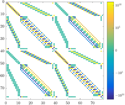
Figure 1: Matrix of the final system of equations in cantilever beam case with $N=39$ and 22 % nonzero elements.

4.2 Positioning of nodes in a complex domain

Meshless methods are advertised as the methods that do not require any topological relations among nodes. That implies that even randomly distributed nodes could be used [19]. However, it is well-known that with regularly distributed nodes one achieves much better results in terms of accuracy and stability [20]. This has also been recently reported for MLSM in a solution of a Navier-Stokes problem [7]. The reason behind the sensitivity regarding the distribution of nodes lies in the generation of shape functions. To construct a stable method well balanced support domains are needed, i.e. the nodes in support domain need to be distributed evenly enough [7]. This condition is obviously fulfilled in regular nodal distributions, but when working with more interesting geometries, the positioning of nodes requires additional treatment. In literature one can find several algorithms for distributing the nodes within the domain of different shapes [21, 22]. In this paper we will use an extremely simple algorithm, introduced in [7] to minimize the variations in distances between nodes in the support domain. The basic idea is to “relax” the nodes based on a potential between them. Since a Gaussian function is a suitable potential and already used as weight in the shape functions, the nodes are translated simply as

$$\delta\vec{p}(\vec{p})=-\sigma_{k}\sum_{i=1}^{N_{S}}\nabla w(\vec{p}-\vec{p_{i}}),$$ (27)

where $\delta\vec{p}$, $\vec{p}_{i}$, $\sigma_{k}$ and $N_{S}$ stand for the translation step of the node, position of $i$-th support node, relaxation parameter and number of support nodes, respectively (Figure 2(a)). After offsets in all nodes are computed, the nodes are repositioned as

$$\vec{p}\leftarrow\vec{p}+\delta\vec{p}(\vec{p}).$$ (28)

Presented iterative process procedure begins by positioning the boundary nodes, which are considered as the definition of the domain and are kept fixed throughout the process.

4.3 h-refinement

Besides flexibility regarding the shape of the domain, nodal refinement is often mandatory to achieve desired accuracy in cases with pronounced differences in stress within the domain. A typical example of such situation is a contact problem [17]. To mitigate the error in areas with high stresses the h-refinement scheme is used., which has already been introduced into different meshless solutions [23, 24]. In context of local RBF approximation the h-refinement has been used in the solution of the Burger’s equation [15], where a quad-tree based algorithm has been used to add and remove child nodes symmetrically around the parent node in transient solution of Burgers’ equation. However, the algorithm presented in  [15] supported only regular nodal distribution. In this paper we generalize it also to irregular nodal distribution.

In each node to be refined, new nodes are added on the half distances between the node itself and its support nodes

$$\vec{p}_{j}^{\;new}=\frac{\vec{p}+\vec{p}_{j}}{2},$$ (29)

where index $j$ indicates $j$-th support node. When adding new nodes, checks are performed if the newly added node is too close to any of the existing nodes; in that case the node is not added. Moreover, if the refined node and support node are both boundary nodes, newly added node is positioned on the boundary (Figure 2(b)). This procedure can be repeated several times if an even more refined domain is desired. These subsequent refinements will be called levels of refinement and will be denoted as level $i$ for the refinement that resulted from $i$ applications of the described algorithm.

(a) Scheme of the relax algorithm.

(b) Scheme of the h-refinement algorithm.

Figure 2: Schemes of algorithms used to improve the quality of the discretization.

The described algorithm follows the concept of meshless methods and as such does not require any special topological relations between nodes to refine a certain part of the computation domain. It is also flexible regarding the dimensionality of the domain, i.e. there is no difference in implementation of 2D or 3D variant of the algorithm.

An example on a non-trivial refinement is demonstrated in Fig. 3, where a domain with a hole is considered. The vicinity of the hole is four times refined and then, to mitigate possible irregularities during refinement, relaxed.

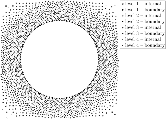
Figure 3: Four levels of the refinement algorithm applied around a hole in a domain after relaxation.

4.4 Asymptotic complexity of MLSM

The asymptotic complexity analysis begins with an assumption that evaluations of basis functions, weights, linear operators and boundary conditions take $O(1)$ time. For simple domain discretization, such as the uniform grid in a rectangle or random positioning, $O(N)$ time is required, where $N$ stands for number of computational nodes. To find the neighbours of each point, a tree based data structure such as kd-tree [6], taking $O(N\log N)$ time to construct and $O(n\log N)$ time to query $n$ closest nodes, is used. The relaxation of nodal positions (see section 4.2) with $I$ iterations costs additional $O(InN\log^{2}N)$ time. Re-finding the support nodes by rebuilding the tree and querying for support nodes once again, requires another $O((N+n)\log N)$ time. Calculation of the shape functions requires $N$ SVD decompositions, each taking $O(nm^{2})$ time, as well as some matrix and vector multiplication of lower complexity. Assembling the matrix takes $O(nN)$ time and assembling the right hand side takes $O(N)$ of time. Then, the system is solved using BiCGSTAB iterative algorithm. The final time complexity is thus $O(InN\log^{2}N+(N+n)\log N+m^{2}nN)+T$, where $T$ stands for the time spent by BiCGSTAB.

For comparison, the complexity of a well-known weak form Element Free Galerking method (EFG) [25] differs from MLSM in construction of the shape functions, whose computation requires $O(Nn_{q}m^{2}n)$ time using EFG method, with $n_{q}$ standing for the number of Gauss integration points per node. Additionally, the number of nonzero elements in the final system of EFG is of order $n_{q}$ times higher than that of MLSM, again increasing the complexity of EFG.

5 Numerical examples

5.1 Cantilever beam

First, the standard cantilever beam test is solved to assess accuracy and stability of the method. Consider an ideal thin cantilever beam of length $L$ and height $D$ covering the area $[0,L]\times[-D/2,D/2]$. Timoshenko beam theory offers a closed form solution for displacements and stresses in such a beam under plane stress conditions and a parabolic load on the left side. The solution is widely known and derived in e.g. [16], giving stresses in the beam as

$$\sigma_{xx} =\frac{Pxy}{I},\quad\sigma_{yy}=0,\quad\sigma_{xy}=\frac{P}{2I}\left(\frac{D^{2}}{4}-y^{2}\right),$$ (30)

and displacements as

$$u =\frac{Py\left(3D^{2}(\nu+1)-4\left(3L^{2}+(\nu+2)y^{2}-3x^{2}\right)\right)}{24EI},$$ (31)

$$v =-\frac{P\left(3D^{2}(\nu+1)(L-x)+4(L-x)^{2}(2L+x)+12\nu xy^{2}\right)}{24EI},$$

where $I=\frac{1}{12}D^{3}$ is the moment of inertia around the horizontal axis, $E$ is Young’s modulus, $\nu$ is the Poisson’s ratio and $P$ is the total load force.

In the numerical solution, traction free boundary conditions are used on the top and bottom of the domain, essential boundary conditions given by (31) are used on the right and traction boundary conditions given by (30) on the left

$$u(L,y) =\frac{Py(2D^{2}(1+\nu)-4(2+\nu)y^{2})}{24EI}$$ (32)

$$v(L,y) =-\frac{L\nu Py^{2}}{2EI}$$ (33)

$$\mu\frac{\partial u}{\partial y}(x,D/2)+\mu\frac{\partial v}{\partial x}(x,D/2)) =0$$ (34)

$$\lambda\frac{\partial u}{\partial x}(x,D/2)+(\lambda+2\mu)\frac{\partial v}{\partial y}(x,D/2) =0$$ (35)

$$-\mu\frac{\partial u}{\partial y}(x,-D/2)-\mu\frac{\partial v}{\partial x}(x,-D/2)) =0$$ (36)

$$-\lambda\frac{\partial u}{\partial x}(x,-D/2)-(\lambda+2\mu)\frac{\partial v}{\partial y}(x,-D/2) =0$$ (37)

$$-\lambda\frac{\partial v}{\partial y}(0,y)-(\lambda+2\mu)\frac{\partial u}{\partial x}(0,y) =0$$ (38)

$$-\mu\frac{\partial u}{\partial y}(0,y)-\mu\frac{\partial v}{\partial x}(0,y) =\frac{P}{2I}((D/2)^{2}-y^{2}).$$ (39)

The problem is solved using MLSM method with $n=9$ or $n=13$ support nodes and Gaussian weight with $\sigma=1$ (see (5)). Two sets of basis functions are considered, 9 monomials

$$\boldsymbol{b}=\{1,x,y,x^{2},y^{2},xy,x^{2}y,xy^{2},x^{2}y^{2}\}$$ (40)

and 9 Gaussian basis functions (see (5) for definition) centred in support nodes. In the following discussions these two choices of basis functions will be referred to as M9 and G9, respectively.

System (21) is solved with BiCGSTAB iterative algorithm [26] with ILUT preconditioning [27]. Values of $L=30\,\mathrm{m}$, $D=5\,\mathrm{m}$, $E=72.1\,\mathrm{GPa}$, $\nu=0.33$ and $P=1000\,\mathrm{N/m}$ were chosen as physical parameters of the problem.

The acquired numerical solution of the cantilever beam problem is shown in Figure 4.

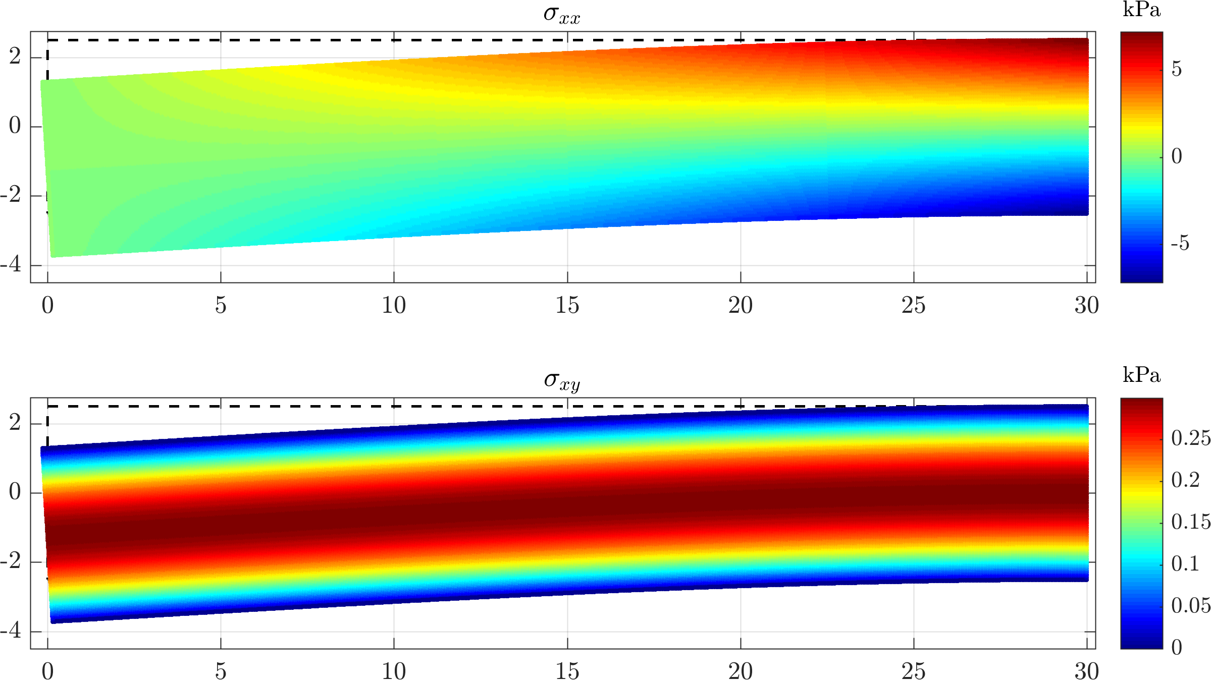
Figure 4: Numerical solution of cantilever beam case. Note that for the sake of visibility the displacements are multiplied by factor $10^{5}$.

The error of the numerical approximation of stresses and displacements is measured in relative discrete $L_{\infty}$ norm, using

$$e_{\infty}(\vec{u}) =\frac{\max_{x\in X}\{\max\{|u(x)-\hat{u}(x)|,|v(x)-\hat{v}(x)|\}\}}{\max_{x\in X}\{\max\{|u(x)|,|v(x)|\}\}}\qquad\text{and}$$ (41)

$$e_{\infty}(\sigma) =\frac{\max_{x\in X}\{\max\{|\sigma_{xx}(x)-\hat{\sigma}_{xx}(x)|,|\sigma_{yy}(x)-\hat{\sigma}_{yy}(x)|,|\sigma_{xy}(x)-\hat{\sigma}_{xy}(x)|\}\}}{\max_{x\in X}\{\max\{|\sigma_{xx}(x)|,|\sigma_{yy}(x)|,|\sigma_{xy}(x)|\}\}},$$ (42)

as error indicators, with $X$ representing the set of all nodes. Convergence with respect to the number of computational nodes is shown in Figure 5. The numerical approximations converge towards the correct solution in stress $(e_{\infty}(\sigma))$ norm as well, with approximately the same convergence rate.

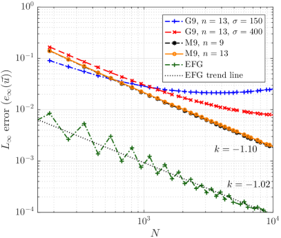
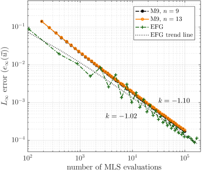
Figure 5: Accuracy of different MLSM setups compared to EFG per number of computational nodes (left) and number of MLS evaluations (right).

It can be seen that monomials converge very regularly with order 1 as expected, while Gaussian functions exhibit slightly worse convergence. Such behaviour has already been reported in solution of diffusion equation, where MLSM with Gaussian basis failed to obtain accurate solution with a high number of computational nodes. More details about the phenomenon and further reading can be found in [28].

The method was compared to the standard Element Free Galerkin (EFG) method [29]. The EFG method used circular domains of influence with radius $d_{I}$ equal to 3.5 times internodal distance, a cubic spline

$$w(\vec{p})=\tilde{w}\left(\frac{\|\vec{p}-\vec{p}_{i}\|}{d_{I}}\right),\quad\tilde{w}(r)=\begin{cases}\frac{2}{3}-4r^{2}+4r^{3}&0\leq r<\frac{1}{2}\\ \frac{4}{3}-4r+4r^{2}-\frac{4}{3}r^{3}&\frac{1}{2}\leq r<1\\ 0&1\leq r\\ \end{cases}$$ (43)

for a weight function, $n_{q}=4$ Gaussian points for approximation of line integrals and $n_{q}=16$ points for approximating area integrals. Lagrange multipliers were used to impose essential boundary conditions.

The performance of EFG with respect to the number of nodes is much better than MLSM. However, a more fair comparison would take into account also a higher complexity of the EFG. This can be achieved by comparing error with respect to the number of MLS evaluations, which is the most time consuming part of the solution procedure. In Figure 5 it is demonstrated that although EFG provides much better results in comparison to MLSM at a given number of nodes, its accuracy becomes comparable to MLSM, when compared per number of MLS evaluations.

To asses the stability of the method regarding the nodal distribution, the following analysis was performed. A regular distribution of points as used in the solution in Figure 4 was distorted by adding a random perturbation to each internal node. Its position is altered by

$$\hat{\vec{p}}\leftarrow\vec{p}+\sigma\vec{U},\qquad\vec{U}\sim\text{Uniform}([0,\delta]^{2}),$$ (44)

where $\delta$ is the distance to the closest node, and measuring the accuracy of the solution with respect to $\sigma$, representing magnitude of the perturbation. An example of original and perturbed node distributions are shown in Figure 6.

Accuracy of the solution with respect to the perturbation magnitude is presented in Figure 7. It is demonstrated that using monomials as a basis with 9 support nodes results in an unstable setup. On the other hand monomials with 13 support nodes are much more stable and equally accurate, while using Gaussian basis with high shape parameter is the most unstable setup. To mitigate the stability issue, a lower shape parameter can be chosen, however, at the cost of accuracy. Regardless of the setup one can expect the solution to be stable at least up to $\sigma\approx 0.1$. Note that using more nodes in support domain can also increase stability. Refer to [7] for more details.

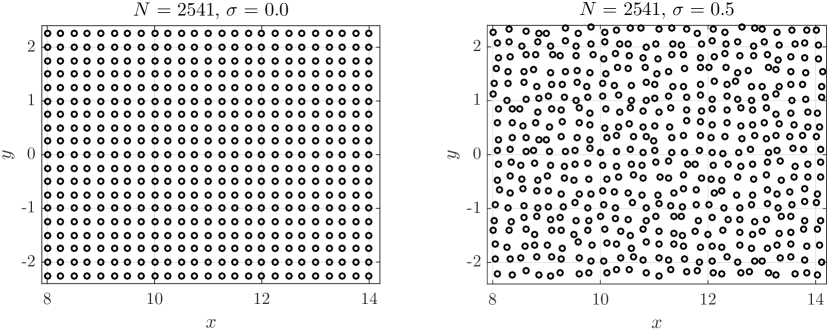
Figure 6: Regular and perturbed node positions, as used in stability analysis.

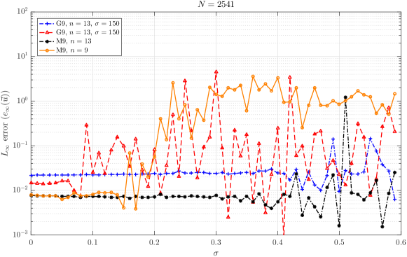
Figure 7: Stability of MLSM with respect to nodal perturbations.

Time spent on each part of the solution procedure is shown in Figure 8. All measurements were performed on a laptop computer with an Intel(R) Core(TM) i7-4700MQ @2.40GHz CPU and with 16 GiB of DDR3 RAM. MLSM is implemented in C++ [18] and compiled using g++ 7.1.7 for Linux with -std=c++14 -O3 -DNDEBUG flags.

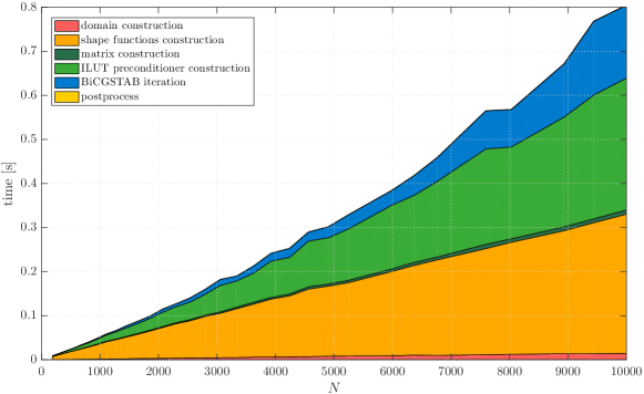
Figure 8: Execution time for different parts of the solution procedure with respect to the number of computational nodes.

It can be seen that solving the system (21) makes up for more than 50 % of total time spent. Around 70 % of that time is spent on computing the preconditioner. The only other significant factor is computing the shape functions taking approximately 40 % of total time. Domain construction and matrix assembly take negligible amounts of time, matching the predictions made by complexity analysis in section 4.4.

To emphasize the generality of MLSM method, a “drilled” domain is considered in the next step. Arbitrarily positioned holes are added to the rectangular domain. The positioning algorithm described in section 4.2 and h-refinement algorithm described in section 4.3 are used to distribute the nodes inside the domain and refine the areas around the holes. The boundary conditions in this example are $\vec{u}=0$ on the right, traction free on the inside of the holes and on top and bottom and uniform load of $P/D$ on the left. The computed solution is shown in Figure 9 along with the ordinary cantilever beam example.

Figure 9: Numerical solution of a drilled cantilever beam case using $N=177618$ nodes. Note that for the sake of visibility the displacements are multiplied by factor $10^{5}$.

Both solutions are coloured using von Mises stress $\sigma_{v}$, computed for the plane stress case as

$$\sigma_{v}=\sqrt{\sigma_{xx}^{2}-\sigma_{xx}\sigma_{yy}+\sigma_{yy}^{2}+3\sigma_{xy}^{2}}.$$ (45)

To further illustrate the generality of the method, an even more deformed domain is considered (Figure 10).

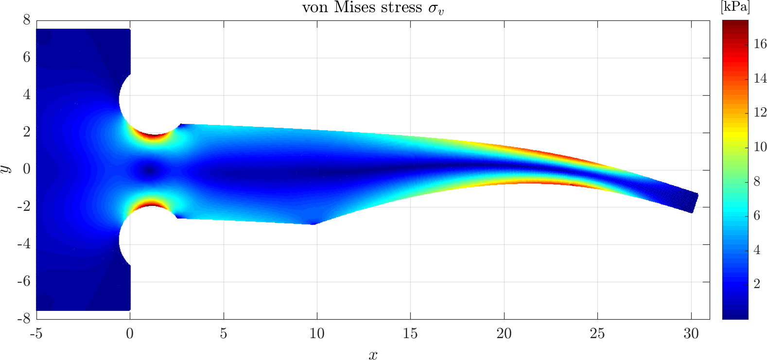
Figure 10: Numerical solution of a irregular cantilever beam using $N=67887$ nodes. Note that for the sake of visibility the displacements are multiplied by factor $10^{5}$.

5.2 Hertzian contact

Another more interesting case arises from basic theory of contact mechanics, called Hertzian contact theory [30]. Consider two cylinders with radii $R_{1}$ and $R_{2}$ and parallel axes pressed together by a force per unit length of magnitude $P$. The theory predicts they form a small contact surface of width $2b$, where

$$b=2\sqrt{\frac{PR}{\pi E^{*}}}$$ (46)

and

$$\frac{1}{R} =\frac{1}{R_{1}}+\frac{1}{R_{2}},$$ (47)

$$\frac{1}{E^{*}} =\frac{1-{\nu_{1}}^{2}}{E_{1}}+\frac{1-{\nu_{2}}^{2}}{E_{2}}.$$ (48)

Elastic modulus and Poisson’s ratio for the first material are denoted with $E_{1}$ and $\nu_{1}$, and with $E_{2}$ and $\nu_{2}$ for the second material. The pressure distribution between the bodies along the contact surface is semi-elliptical, i.e. of the form

$$p(x)=\begin{cases}p_{0}\sqrt{1-\frac{x^{2}}{b^{2}}};&|x|\leq b\\ 0;&\text{otherwise}\end{cases},\qquad p_{0}=\sqrt{\frac{PE^{*}}{\pi R}}.$$ (49)

A problem can be reduced to two dimensions using plane stress assumption. A special case of this problem is when $E_{1}=E_{2}$, $\nu_{1}=\nu_{2}$ and $R_{2}\to\infty$, describing a contact of a cylinder and a half plane. This is the second numerical example tackled in this paper. The setup is ideal for testing the refinement, since a pronounced difference in behaviour of numerical solution near the contact in comparison to the rest of the domain is expected.

A displacement field $\vec{u}$ satisfying (15) on $(-\infty,\infty)\times(-\infty,0)$ with boundary conditions

$$\vec{t}(x,0)=-p(x)\vec{\jmath}$$ (50)

$$\lim_{x,y\to\infty}\vec{u}(x,y)=0.$$ (51)

is sought. Vector $\vec{t}$ represents traction force on the surface and $\vec{\jmath}=(0,1)$ the upwards direction. Analytical solution for internal stresses in the plane in general point $(x,y)$ is calculated using the method of complex potentials [31] and the stresses are given in terms of $m$ and $n$, defined as

$$m^{2} =\frac{1}{2}\left(\sqrt{\left(b^{2}-x^{2}+y^{2}\right)^{2}+4x^{2}y^{2}}+b^{2}-x^{2}+y^{2}\right),$$ (52)

$$n^{2} =\frac{1}{2}\left(\sqrt{\left(b^{2}-x^{2}+y^{2}\right)^{2}+4x^{2}y^{2}}-(b^{2}-x^{2}+y^{2})\right),$$ (53)

where $m=\sqrt{m^{2}}$ in $n=\operatorname{sgn}(x)\sqrt{n^{2}}$. The stresses are then expressed as

$$\sigma_{xx} =-\frac{p_{0}}{b}\left[m\left(1+\frac{y^{2}+n^{2}}{m^{2}+n^{2}}\right)+2y\right]$$ (54)

$$\sigma_{yy} =-\frac{p_{0}}{b}m\left(1-\frac{y^{2}+n^{2}}{m^{2}+n^{2}}\right)$$ (55)

$$\sigma_{xy} =\sigma_{yx}=\frac{p_{0}}{b}n\left(\frac{m^{2}-y^{2}}{m^{2}+n^{2}}\right).$$ (56)

Numerically the problem is solved by truncating the infinite domain to a rectangle $[-H,H]\times[-H,0]$ for large enough $H$ and setting the essential boundary conditions $\vec{u}=0$ everywhere but on the top boundary. The top boundary has a traction boundary condition with normal traction given by $p(x)$ and no tangential traction. An illustration of the problem domain along with the boundary conditions is given in Figure 11.

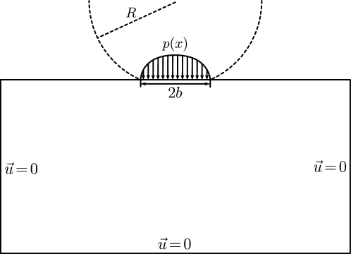
Figure 11: Domain and boundary conditions of considered contact problem.

The described contact problem is solved numerically and the error is measured between calculated and given stresses in relative $L_{\infty}$ norm as before, using

$$e_{\infty}=\max_{x\in X}\{\max\{|\sigma_{xx}(x)-\hat{\sigma}_{xx}(x)|,|\sigma_{yy}(x)-\hat{\sigma}_{yy}(x)|,|\sigma_{xy}(x)-\hat{\sigma}_{xy}(x)|\}\}/p_{0}$$

as an error indicator. Values $P=543\,\mathrm{N/m}$, $E_{1}=E_{2}=72.1\,\mathrm{GPa}$, $\nu_{1}=\nu_{2}=0.33$, $R_{1}=R=1\,\mathrm{m}$ were chosen for the physical parameters of the problem. These values yield contact half-width $b=0.13\,\mathrm{mm}$ and peak pressure $p_{0}=2.6\,\mathrm{MPa}$. A value of $H=10\,\mathrm{mm}$ for domain height is chosen, approximately 38 times greater than width of the contact surface. Convergence of the method is shown in Figure 12.

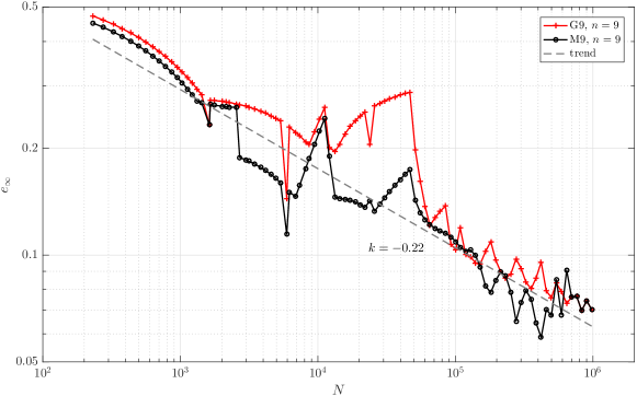
Figure 12: Convergence of MLSM when solving the described Hertzian contact problem.

It is clear that the convergence of the method is very irregular and slow. This is to be expected, as $N=10^{6}$ means only approximately 30 nodes positioned within the contact surface, and that naturally leads to large changes as a change of a single node bears a relatively high influence. Another problem is that the boundary conditions are only continuous, and exhibit no higher regularity, not even Lipschitz continuity. The accuracy of the approximation may seem bad, but is in fact comparable to the cantilever beam case. Using the comparable value of $N=30\cdot 15=450$ nodes in the contact area $[-b,b]\times[-b,0]$ it can be seen from Figure 5 that the approximation using this number of nodes in cantilever beam case achieved very similar results.

The total error of the approximation is composed of two main parts, the truncation error due to the non-exact boundary conditions and the discretization error, due to solving a discrete problem instead of the continuous one. First, we analyse the total error in terms of domain height $H$. A graph showing the total error with respect to domain height $H$ is shown in Figure 13.

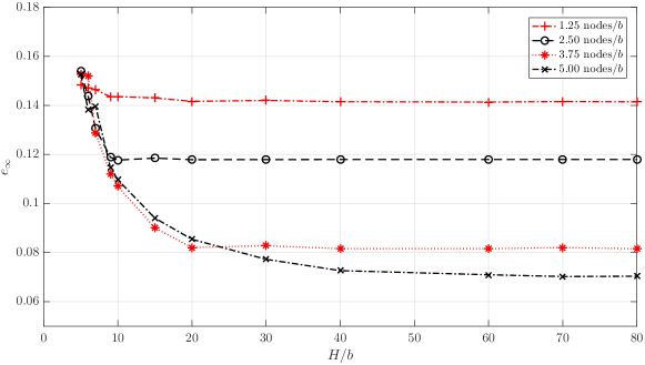
Figure 13: Total error with respect to domain size at different discretization densities.

The total error decreases as domain height increases, regardless of the discretization density used. However, as soon as truncation error becomes lower than discretization error, increasing the height further yields little to no gain in total error. The higher the discretization density is, the later this happens. When convergence of a method stops or significantly decreases in order, an error limit imposed by the truncation error was reached.

It soon becomes impossible to uniformly increase discretization density due to limited resources, and the immediate solution is to refine the discretization in the contact area with the h-refinement algorithm introduced in section 4.3. A domain of height $H=1\,\mathrm{m}\approx 75\,000b$ is chosen. Primary refinement is done in rectangle areas of the form

$$[-hb,hb]\times[0,hb],\text{ for }h\in\{1000,500,200,100,50,20,10,5,4,3,2\},$$

and secondary refinement around points $\pm b$ on the surface is done in rectangle areas

$$[c-hb,c+hb]\times[-hb,0],\text{ for }c=\pm b\text{ and }h\in\{0.4,0.3,0.2,0.1,0.05,0.0025\}.$$

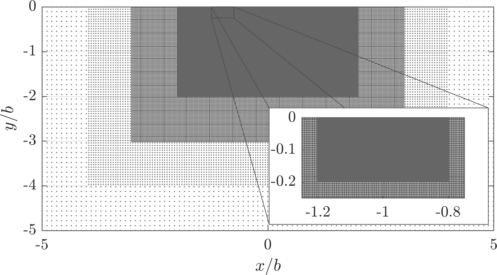
(a) A part of the refined domain.

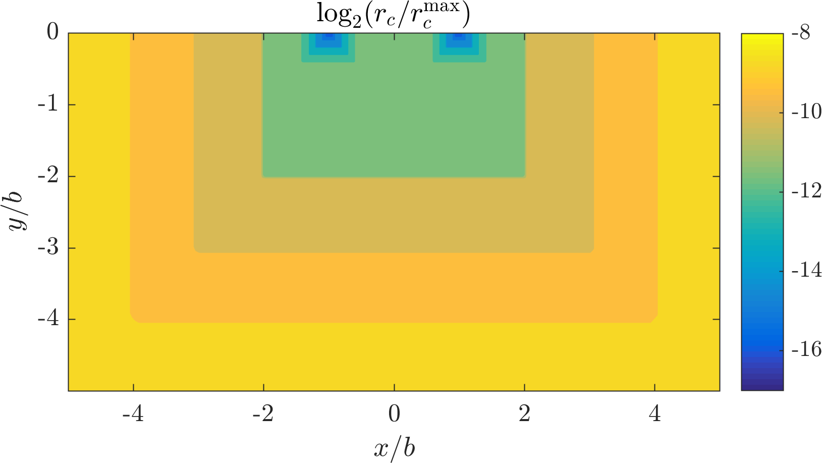
(b) Discretization density of the refined domain.

Figure 14: An example of 17-times refined domain used in solution of the described Hertzian contact problem.

The refined domain as described above is shown in Figure 14. This domain was used to solve the considered contact problem. Different levels of secondary refinement were tested to prove that refinement helps with accuracy. Convergence of the method on the refined domain is shown in Figure 15.

Figure 15: Convergence of MLSM at different refine levels.

Comparing Figure 15 to Figure 12, it can be seen that refinement greatly improves the accuracy of the method. Using $N=10^{6}$ nodes without refinement yields worse results than $N=10^{4}$ nodes with only primary refinement. Each additional level of secondary refinement helps to decrease the error even further while keeping the same order of convergence. A solution of the problem on the final mesh is shown in Figure 16.

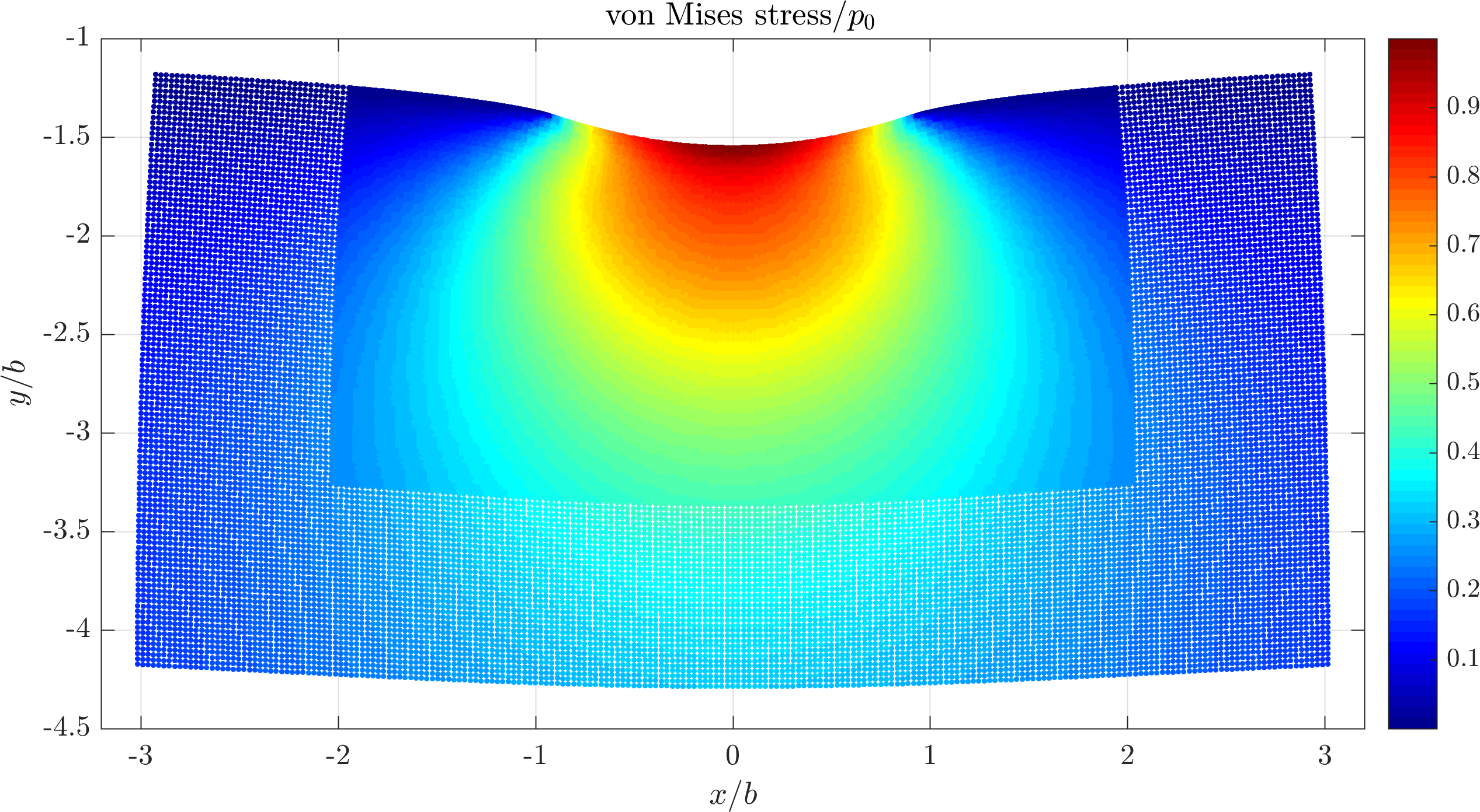
Figure 16: Numerical solution of the described Hertzian contact problem. Note that for the sake of visibility the displacements are multiplied by factor of $5\cdot 10^{3}$.

6 Conclusions

A MLSM solution of a linear elasticity problem on regular and irregular domains with a refined nodal distribution of two different numerical examples is presented in this paper. The method is analysed in terms of accuracy by comparison against available closed form solutions and by comparison against weak form EFG method. The convergence of the method is evaluated with respect to the number of computational nodes, selection of different basis functions, different refinement strategies and different boundary conditions. MLSM is also analysed from complexity point of view, first, theoretically, and then also experimentally by timing the computer execution time of all main blocks of the method. It is clearly demonstrated that the method is accurate and stable. Furthermore, it is demonstrated that nodal adaptivity is mandatory when solving contact problems in order to obtain accurate results and that the proposed MLSM method can handle extensive refinement with the smallest internodal distance being $2^{17}$ times smaller than the initial one. It is also demonstrated that proposed MLSM configuration can handle computations in complex domains.

In our opinion the presented meshless setup can be used, not only to solve academic cases with the sole goal to show excellent convergences, but also in more complex engineering problems. The C++ implementation of presented MLSM is freely available at [18].

In future work we will continue to develop a meshless solution of a contact problem with a final goal to simulate a crack propagation due to the fretting fatigue [17] in a general 3D domain with added p-adaptivity to treat singularities near the crack tip.

References

- [1] O. C. Zienkiewicz, R. L. Taylor, The Finite Element Method: Solid Mechanics, Butterworth-Heinemann, 2000.
- [2] J. H. Hattel, P. N. Hansen, A control volume-based finite difference method for solving the equilibrium equations in terms of displacements, Applied Mathematical Modelling 19 (1994) 210–243.
- [3] Y. D. Freyer, C. Bailey, M. Cross, C.-H. Lai, A control volume procedure for solving the elastic stress-strain equations on an unstructured mesh, Applied Mathematical Modelling 15 (1991) 639–645.
- [4] Y. Chen, J. D. Lee, A. Eskandarian, Meshless methods in solid mechanics, Springer, New York, NY, 2006.
- [5] B. Mavrič, B. Šarler, Local radial basis function collocation method for linear thermoelasticity in two dimensions, International Journal of Numerical Methods for Heat and Fluid Flow 25 (2015) 1488–1510.
- [6] R. Trobec, G. Kosec, Parallel scientific computing: theory, algorithms, and applications of mesh based and meshless methods, Springer, 2015.
- [7] G. Kosec, A local numerical solution of a fluid-flow problem on an irregular domain, Advances in Engineering Software.
- [8] G. Kosec, R. Trobec, Simulation of semiconductor devices with a local numerical approach, Engineering Analysis with Boundary Elements 50 (2015) 69–75.
- [9] C. A. Wang, H. Sadat, C. Prax, A new meshless approach for three dimensional fluid flow and related heat transfer problems, Computers and Fluids 69 (2012) 136–146.
- [10] S. Li, K. W. Liu, Meshfree and particle methods and their applications, Applied Mechanics Reviews 55 (2002) 1–34.
- [11] S. N. Atluri, The Meshless Method (MLPG) for Domain and BIE Discretization, Tech Science Press, Forsyth, 2004.
-
[12]
J. Zhang, H. Chen, C. Cao,
A graphics processing
unit-accelerated meshless method for two-dimensional compressible flows,
Engineering Applications of Computational Fluid Mechanics 11 (1) (2017)
526–543.
arXiv:http://dx.doi.org/10.1080/19942060.2017.1317027, doi:10.1080/19942060.2017.1317027.
URL http://dx.doi.org/10.1080/19942060.2017.1317027 -
[13]
W. Li, G. Song, G. Yao,
Piece-wise
moving least squares approximation, Applied Numerical Mathematics 115 (2017)
68–81.
doi:10.1016/j.apnum.2017.01.001.
URL http://linkinghub.elsevier.com/retrieve/pii/S0168927417300016 -
[14]
K. Kovářík, S. Masarovičová, J. Mužík, D. Sitányiová,
A
meshless solution of two dimensional multiphase flow in porous media,
Engineering Analysis with Boundary Elements 70 (2016) 12–22.
doi:10.1016/j.enganabound.2016.05.008.
URL http://linkinghub.elsevier.com/retrieve/pii/S0955799716300911 - [15] G. Kosec, B. Šarler, H-adaptive local radial basis function collocation meshless method, CMC: Computers, Materials, and Continua 26 (3) (2011) 227–253.
- [16] W. S. Slaughter, The linearized theory of elasticity, Springer Science & Business Media, 2012.
- [17] K. Pereira, S. Bordas, S. Tomar, R. Trobec, M. Depolli, G. Kosec, M. Abdel Wahab, On the convergence of stresses in fretting fatigue, Materials 9 (8) (2016) 639.
-
[18]
G. Kosec, M. Kolman, J. Slak,
Utilities for solving pdes
with meshless methods (2016).
URL https://gitlab.com/e62Lab/e62numcodes.git - [19] K. Reuther, B. Sarler, M. Rettenmayr, Solving diffusion problems on an unstructured, amorphous grid by a meshless method, International Journal of Thermal Sciences 51 (2012) 16–22.
- [20] J. Amani, M. Afshar, M. Naisipour, Mixed discrete least squares meshless method for planar elasticity problems using regular and irregular nodal distributions, Engineering Analysis with Boundary Elements 36 (2012) 894–902.
- [21] R. Löhner, E. Oñate, A general advancing front technique for filling space with arbitrary objects, International Journal for Numerical Methods in Engineering 61 (12) (2004) 1977–1991.
- [22] Y. Liu, Y. Nie, W. Zhang, L. Wang, Node placement method by bubble simulation and its application, CMES: Computer Modeling in Engineering & Sciences 55 (1) (2010) 89.
- [23] N. A. Libre, A. Emdadi, E. J. Kansa, M. Rahimian, M. Shekarchi, A stabilised rbf collocation scheme for neumann type boundary conditions., CMES: Computer Modeling in Engineering & Sciences 24 (2008) 61–80.
- [24] G. C. Bourantas, E. D. Skouras, G. C. Nikiforidis, Adaptive support domain implementation on the moving least squares approximation for mfree methods applied on elliptic and parabolic pde problems using strong-form description, CMES: Computer Modeling in Engineering & Sciences 43 (2009) 1–25.
- [25] T. Belytschko, Y. Y. Lu, L. Gu, Element-free galerkin methods, Int. J. Numer. Methods Eng. 37 (2) (1994) 229–256.
- [26] H. A. Van der Vorst, Bi-CGSTAB: A fast and smoothly converging variant of Bi-CG for the solution of nonsymmetric linear systems, SIAM Journal on scientific and Statistical Computing 13 (2) (1992) 631–644.
- [27] Y. Saad, ILUT: A dual threshold incomplete LU factorization, Numerical linear algebra with applications 1 (4) (1994) 387–402.
- [28] G. Kosec, P. Zinterhof, Local strong form meshless method on multiple graphics processing units, CMES: Computer Modeling in Engineering & Sciences 91 (5) (2013) 377–396.
- [29] V. P. Nguyen, T. Rabczuk, S. Bordas, M. Duflot, Meshless methods: a review and computer implementation aspects, Mathematics and computers in simulation 79 (3) (2008) 763–813.
- [30] J. A. Williams, R. S. Dwyer-Joyce, Contact between solid surfaces, Modern tribology handbook 1 (2001) 121–162.
- [31] E. M’Ewen, Stresses in elastic cylinders in contact along a generatrix (including the effect of tangential friction), The London, Edinburgh, and Dublin Philosophical Magazine and Journal of Science 40 (303) (1949) 454–459. doi:10.1080/14786444908521733.