The mini-GWAC optical follow-up of the gravitational wave alerts:
results from the O2 campaign and prospects for the upcoming O3 run.

Abstract

The second (O2) observational campaign of gravitational waves (GW) organized by the LIGO/Virgo Collaborations has led to several breakthroughs such as the detection of gravitational wave signals from merger systems involving black holes or neutrons stars. During O2, 14 gravitational wave alerts were sent to the astronomical community with sky regions covering mostly over hundreds of square degrees. Among them, 6 have been finally confirmed as real astrophysical events. Since 2013, a new set of ground-based robotic telescopes called GWAC (Ground Wide field Angle Cameras) and its pathfinder mini-GWAC have been developed to contribute to the various challenges of the multi-messenger and time domain astronomy. The GWAC system is built up in the framework of the ground-segment system of the SVOM mission that will be devoted to the study of the multi-wavelength transient sky in the next decade. During O2, only the mini-GWAC telescope network was fully operational. Due to the wide field of view and fast automatic follow-up capabilities of the mini-GWAC telescopes, they were well adapted to efficiently cover the sky localization areas of the gravitational wave event candidates. In this paper, we present the mini-GWAC pipeline we have set up to respond to the GW alerts and we report our optical follow-up observations of 8 GW alerts detected during the O2 run. Our observations provided the largest coverage of the GW localization areas in a short latency made by any optical facility. We found tens of optical transient candidates in our images, but none of those could be securely associated with any confirmed black hole - black hole merger event. Based on this first experience and the near future technical improvements of our network system, we will be more competitive to detect the optical counterparts from some gravitational wave events that will be detected during the upcoming O3 run, especially those emerging from binary neutron star mergers.

¹Key Laboratory of Space Astronomy and Technology, National Astronomical Observatories, Chinese Academy of Sciences, Beijing 100101
²LAL, Univ. Paris-Sud, CNRS/IN2P3, Université Paris-Saclay, F-91898 Orsay, France
³APC, Univ Paris Diderot, CNRS/IN2P3, CEA/lrfu, Obs de Paris, Sorbonne Paris Cité, France
⁴CEA Saclay, DRF/IRFU/Département d’astrophysique, 91191 Gif-sur-Yvette, France
⁵School of Astronomy and Space Science, University of Chinese Academy of Sciences, 101408 Beijing
⁶Université de Toulouse, IRAP 14 Av. Edouard Belin, F-31000 Toulouse France
⁷Institut de Recherche en Astrophysique et Planétologie (IRAP), UPS-OMP, Toulouse, France
⁸Department of Physics and GXU-NAOC Center for Astrophysics and Space Sciences, Guangxi University, Nanning 530004, China
⁹Institute of High Energy Physics/CAS, 19B YuquanLu, Beijing, 100049 , China
¹⁰School of Physics and Electronic Information, Huaibei Normal University, Huaibei 235000, China
^† dturpin@nao.cas.cn

accepted on Aug. 2019 in Research in Astronomy and Astrophysics

Key words: gravitational waves – methods: observational – stars: optical transients – (stars:)

1 Introduction

The new generation of gravitational wave (GW) LIGO/Virgo detectors have given us an access to a new physics on the compact and extreme objects in the Universe such as the black holes (BH) or the neutron stars (NS) with unprecedented details, see for example (Abbott et al., 2016a). In 2015, the O1 GW observational campaign, marked the birth of the gravitational wave astronomy with the first two detections of GW signals produced by the coalescence of black holes bounded in binary systems (BBH) (Abbott et al., 2016b, c). A search for electromagnetic counterparts from these merger systems was performed without any significant result. While any electromagnetic counterpart from a BBH merger event is very unlikely, it has not been completely ruled out by some models under particular conditions (Loeb, 2016; Zhang et al., 2016; Zhang, 2016; Perna et al., 2016; de Mink & King, 2017). In addition to that, the poor localization of these GW events and the long delay of the alert communication dramatically reduced the detection capabilities of the electromagnetic facilities. From November 2016 to August 2017, the O2 run has been effective for almost one year with a release of 14 alerts to the external partners of the LIGO/Virgo Collaborations (LVC). This leads to new discoveries of gravitational waves from compact mergers (Abbott et al., 2019). In particular, on 17^th August 2017, the discovery of the GW signal GW170817 emitted, for the first time, from the inspiral and the merger of two neutrons stars (BNS) marked the dawn of the multi-messenger astronomy (Abbott et al., 2017a, b, c). Two matter ejecta were identified after this merger. First, almost simultaneously to the GW signal, a short gamma-ray burst (sGRB), GRB170817A (Goldstein et al., 2017), and much later its associated X-ray and radio afterglows as long as the relativistic ejecta heats up its surrounding environment (for a review on sGRB see Berger, 2014, and references therein). Secondly, about 10 hours after the GW trigger time, thanks to the intensive follow-up observations made by various optical facilities, an isotrotropic ejecta was also clearly identified as the signature of r-processes occuring in a so-called kilonova ejecta as predicted years ago by several authors (Li & Paczyński, 1998; Kulkarni, 2005; Metzger et al., 2010; Metzger, 2017, for a recent review). GW170817 permits to validate for the first time the merger model proposed decades ago to explain the short gamma-ray burst phenomena (Paczyński, 1986; Eichler et al., 1989; Paczyński, 1991). Beyond this remarkable result, the O2 run demonstrated the importance of having a third detector with the advanced Virgo, entering in science mode, to significantly reduce the error on the localization of some GW events (Abbott et al., 2017a, d). However, the Virgo detector only joined the last month of the O2 run, thus, a large majority of the O2 GW candidates remained poorly localized. According to the online LVC detection pipeline, the median size of the sky localization error box of the O2 GW alerts was $\mathrm{\sigma_{90\%}=1725\leavevmode\nobreak\ deg^{2}}$ (Abbott et al., 2019). Practically speaking, in the electromagnetic domain, with such localization constraint and depending on the distance of the event, the discovery potential of the telescopes having relatively small field of views (typically FoV $<$1 sq.deg.) and usually operated in pointing mode is very low. As a consequence, it was primordial to conduct efficient electromagnetic follow-ups using optimized strategies for both small and wide field of view telescopes. The electromagnetic counterpart searches were therefore performed through various observational strategies including archival data analysis, prompt searches with all-sky instruments, wide-field tiled searches, targeted searches of potential host galaxies with small field of view facilities, and deep follow-up of individual sources. In the optical domain, the wide field instruments have the advantage of being able to cover a large fraction of the GW error boxes in a minimum amount of time.
Since 2013, the Ground-based Wide field Angle Cameras (GWAC) telescopes are under development at the Xinglong Observatory in China to prepare the future ground segment of the SVOM mission dedicated to the study of the transient sky in 2021 with both spaced-based and ground-based multi-wavelength instruments (Wei et al., 2016). Due to the design of its extreme wide field of view ($25^{\circ}\times 25^{\circ}$), the GWAC telescopes are well suited for the optical follow-up of the GW candidates. They have the capability to perform routine observations of the transient sky every night and, as being robotic, they are able to cover very rapidly a significant portion of the GW localization regions. These two specificities allowed us to conduct the first extensive optical follow-up of gravitational wave events, searching for early optical counterparts, from China. For the O2 GW run, our optical follow-up campaign was performed with the pathfinder telescopes mini-GWAC.

In this paper we present our optical follow-up system of the O2 GW alerts and the results of our campaign. We will firstly describe, in section 2, our mini-GWAC telescopes used during O2. We then present, in section 3, our transient research program set up to respond to any multi-messenger alerts. The results of our follow-up observations of the gravitational wave alerts are shown in section 4. In section 5, we will discuss the improvements of our detection capabilities for the upcoming O3 run. Finally, we draw our conclusion in section 6.

2 The mini-GWAC telescopes

In 2013, a GWAC pathfinder, called mini-GWAC, has been developed in order to test and validate both the hardware and the data processing pipeline of the future GWAC system.
Located at the Xinglong Observatory (lat = 40^∘23’39”N, lon = 117^∘34’30”E) and founded by the National Astronomical Observatories (NAOC, Chinese Academy of Sciences), the mini-GWAC network is composed of 6 mounts. Each mount is equipped with 2 Canon 85/f1.2 cameras with an aperture of 7 cm, as shown in Figure 1.

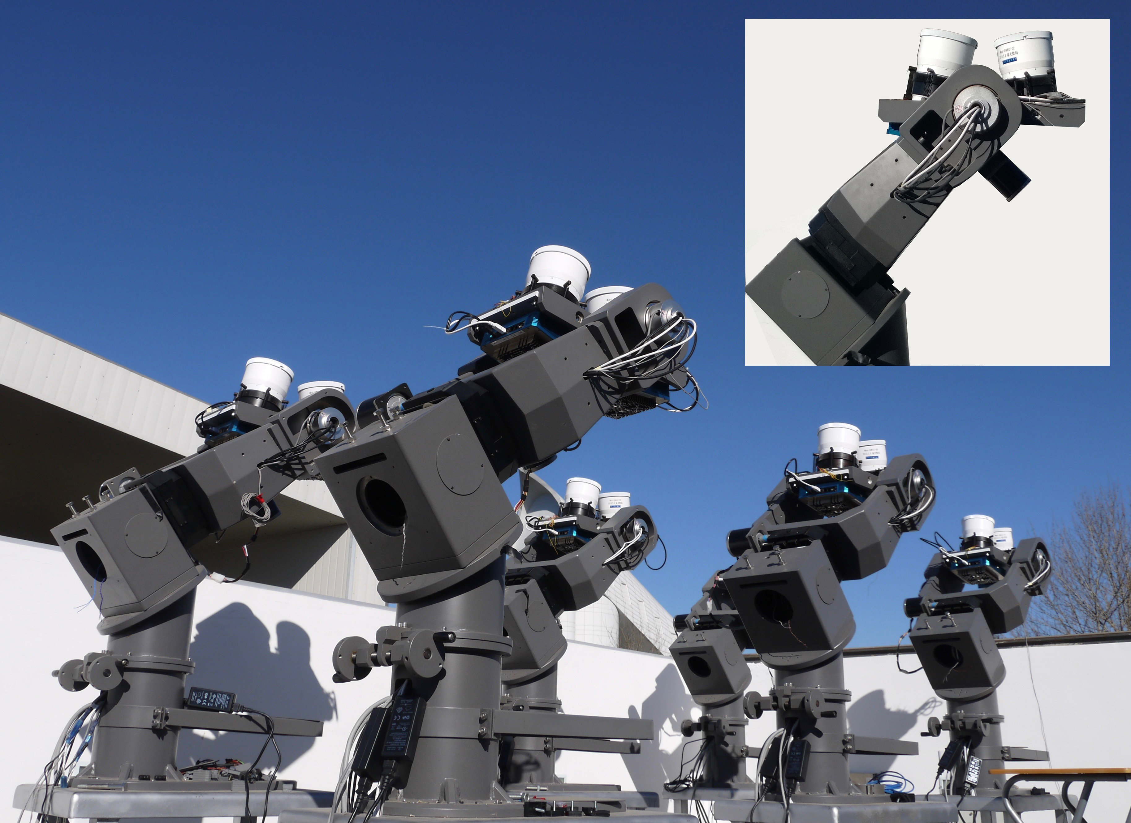
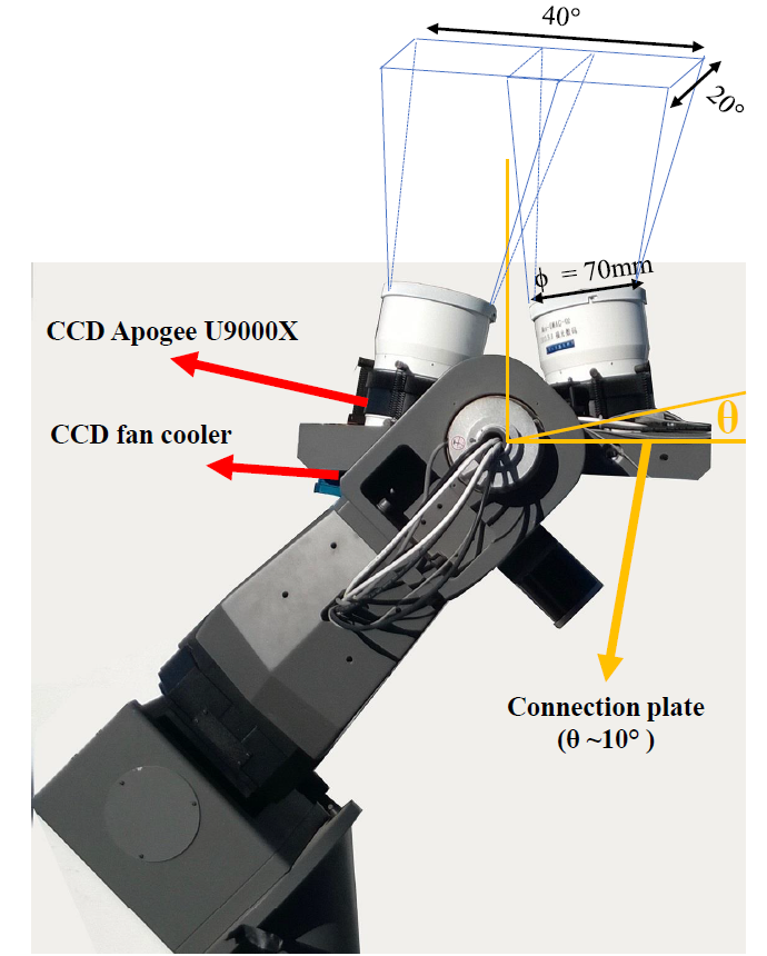
Figure 1: (left) The mini-GWAC telescope farm, located at the Xinglong Observatory, includes 6 mounts and 12 Canon 85/f1.2 cameras. (Right) Each mount is equipped with 2 cameras with a field of view (FoV) of 20${}^{\circ}\times 40^{\circ}$ for a total FoV for the whole system of about 5000 sq.deg (about 1/4 of the Northern sky). The image cadency is 15 seconds.

For each camera, the detector is a CCD Apogee U9000X with an image cadence of 15 seconds (exposure=10s, read-out=5s) and a readout noise of 12 electrons RMS at 1 MHz. Each camera is cooled down to -45^∘ C with respect to the local environment temperature with a thermoelectric cooler system with forced air. Two cameras are installed on a connection plate with a fix angle and are paved in a rectangle sky field. With such a configuration, one mount has a field of view of 20 degrees along the longitude direction and 40 degrees along the latitude one. This results in a field of view (FoV) of 800 square degrees per mount. Combining the network of the 6 mini-GWAC mounts, the overall FoV is about 5000 square degrees. From the mini-GWAC single images, a typical limiting (unfiltered) magnitude of about 12 is obtained in a dark night without clouds. The mini-GWAC telescopes have been designed with an extreme wide field of view and a small imaging cadence in order to mainly search for short-time scale optical transients (OTs). The first light of mini-GWAC was obtained on October 2015 during the O1 GW science run and the first follow-up of a GW event was made for GW151226 (Wei et al., 2015). A specific data processing pipeline has been developed to automatically detect in real-time OT candidates in the images.

Each mini-GWAC telescope is operated in a sky survey mode. A pre-planed sky monitoring strategy is adopted, so that the all sky is partitioned into several fixed grids whose sizes are based on each mount’s FoV, see Figure 2.

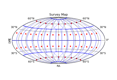
Figure 2: The sky, in Equatorial coordinates, fragmented in grids of equal area according to the mini-GWAC per mount’s field of view. Each night, observations are performed in a survey mode following the grid pointings (red dots) with a maximum of three grids per mount to be visited. At the position of the Xinglong observatory the grids with declination $\delta<20^{\circ}$ S are never observable.

During a night, each telescope starts to monitor one assigned sky grid until this one is no longer observable. For a given mount, each observed grid is chosen to optimize its observational conditions, i.e. a high elevation above the horizon, a minimum distance to the moon of 20^∘ when the moon phase is lower than 0.5 (half moon, 1 is the full moon phase) and 30^∘ otherwise and also having no overlap with the other grid pointings observed by other mini-GWAC telescopes. Once the first grids are no longer observable, the mounts automatically slew to observe new grids following the same observational strategy. Typically, no more than three different grids are usually monitored by a single mount in a single night. During the observations, each camera is automatically focused to make the image quality at its best level following the method developed by Huang et al. (2015). The images taken by all the mini-GWAC cameras are then analyzed in real-time and independently camera per camera.

3 The mini-GWAC optical transient search program

During the mini-GWAC survey, we simultaneously run a program dedicated to the discovery of new optical transient sources in our images. This search program relies on two main steps: the detection of the OT candidates and then their classification using various filters. The OTs that can be detected in our mini-GWAC images originate from two classes of triggers: the external triggers such as the GW alerts or the internal triggers, i.e the alerts produced by the GWAC system itself after the detection of an OT in real-time by chance in our images. Typically, in the external trigger case, we expect to catch the early phases of the GRB afterglow emission, some supernovae previously discovered by other groups, galactic explosive events such as cataclysmic variables (CVs), tidal disruption events or the optical counterparts from GW events. For the internal triggers, we expect to rather detect near-Earth objects, uncatalogued flaring stars, supernovae, galactic transients and also many unexpected optical transients as the time-domain covered by mini-GWAC/GWAC (less than the minute timescale) is still largely unexplored yet in the optical domain.
The analysis of the images is performed in real-time using two transient search methods, i.e. the catalog cross-matching method and the difference image analysis (DIA). These methods usually yield the detection of dozens of optical transient candidates by each mini-GWAC telescope every night. In the following section, we briefly describe our two detection pipelines.

3.1 The online mini-GWAC data processing

3.1.1 The catalog cross-matching method

A specific pipeline to detect short-living transients in the mini-GWAC images has been developed mainly from the IRAF package and SourceExtractor software (Bertin & Arnouts, 1996). The method is based on the comparison of the transient candidate positions found in the images with those of objects already catalogued in public archives. The catalog used in our pipeline is a mixture of the USNO B1.0 catalog and the stellar catalog produced by SourceExtractor using our reference images. The USNO B1.0 catalog has been chosen because of its all-sky coverage with reasonable astrometric measurements and a high completeness down to V=16, corresponding to the nominal design for the GWAC sensitivity. The reference images are obtained by co-adding 10 images of high quality from the same grid region. These images are automatically picked-up in the mini-GWAC image database and selected based on the quality of their stellar point spread function (PSF), background brightness and atmospheric transparency.
Note that the coma is quite serious at the extreme edge of the mini-GWAC images which affect our detection efficiency. We estimated a loss of about 0.5 mag in our sensitivity threshold between OTs detected in the extreme edge of the image, where the PSF of stars can slightly deviate from a 2D gaussian profile, and the inner part of it (typically the 2k x 2k part of the image). A new optical source is detected in our images if it fulfills the following criteria:

• (i) The candidate must not be detected in the reference image with a signal-to-noise ratio greater than SNR = 5, while it is in the night images.

• (ii) In order to exclude some moving objects, the candidate shall be detected in at least two continuous images without any apparent shift in its position.

• (iii) There is no any minor planet object with a brightness larger than 13 mag near the location of the candidate. The choice of this limiting magnitude is made according to the sensitivity of the mini-GWAC telescopes.

• (iv) There is no any defect in the CCD camera at the location of the candidate.

• (v) The PSF and the ellipticity of any candidate shall be stellar-like profile (2D gaussian profile with a limited deviation). At the edge of the image, this criterion reduces our detection efficiency for faint sources.

If an OT candidate is confirmed as being an uncatalogued source, then our pipeline allows to sample the optical emission of the transient in a short time resolution of 15 seconds. In order to improve our detection capabilities, a stacking analysis based on a group of ten images is also processed in parallel. This allows to increase the signal to noise ratio (SNR) of faint objects to detect them at the edge of our camera sensitivity but with a lower time resolution. For these faint OTs we will finally reach a time resolution from several minutes to a few hours.

3.1.2 Differential image analysis

The difference image analysis (DIA) is made by following three steps:

• (i) an image alignment between the reference and the night images.

• (ii) the difference between the two images to obtain a residual image.

• (iii) the transient candidate selection after the residual analysis.

First, for the image alignment method, we used the Becker implementation of the Alard (2000) algorithm finely tuned for the mini-GWAC data. All the images (reference and night) used for DIA are truncated from the $3056\times 3056$px of the raw image to $2001\times 2001$px to avoid the bad PSF quality near the edge of the images. Before the subtraction, flux and PSF calibrations are operated on both images to obtain the best residuals possible. Once the subtraction is made, the transient selection program employs a supervised machine learning routine based on a random forest algorithm to preliminary classify the spurious points in the residual images. The reference images are taken days before the trigger time to ensure, as much as possible, that no optical precursor is present in our data at the OT candidate position. Then, the OT selection criteria follow the same rules than the ones described above for the catalog cross-matching method. With such DIA method we can also apply a stacking analysis in the images to enhance our optical flux sensitivity.

3.2 Optical transient classification

Once an image is processed, a list of preliminary OT candidates is automatically established by comparing the subsequent results of the two detection pipelines. These candidates, labeled as OT1 candidates, are usually composed of non astrophysical sources, fake optical transients such as minor planets or variable stars and a few amount of possibly genuine optical transient sources either in a rising or a fading phase.
The search for OTs then implies to carefully filter the OT1 candidates sample out of all the fakes through several steps. The first series of selection criteria mostly rely on the PSF analysis of the candidates, additional checks in other all sky catalogs such as 2MASS, SDSS9, DSS2, and their detection in a time series of at least 2 images. From this step, most of the OT1 candidates are mainly classified as non-astrophysical sources ( i.e hot pixel, crosstalk, cosmic-rays, dust and CCD artifacts, moving debris etc.) or astrophysical sources but identified as moving objects like minor planets. The candidates that pass these series of filters are then labeled as OT2 candidates, the others are automatically rejected.
The OT2 candidates can still be a mix of fake OTs that were not well filtered during the first steps and few (or even zero) real OTs. Therefore, we analyze them one by one through a human-eye check (PSF matching, lightcurve and public archive check). For the candidates judged by our duty scientist as being promising, we trigger fast extra multi-wavelength follow-up observations (Yang et al., 2019, in prep.) at deeper magnitudes (typically R $\sim$ 19 for an exposure = 120 seconds) with two dedicated 60 cm robotic telescopes (GWAC-F60A/B, UBVRI filters, jointly operated by the NAOC and the Guangxi University). Based on this set of informations, we may confirm some of the OT2 candidates as being genuine optical transients, while the others are finally rejected. The remaining confirmed OTs are therefore labeled OT3 candidates. At this stage, we usually reduce the initial number of candidates per night and per telescope from dozens to a very few (including zero) for the mini-GWAC system.
The OT3 candidates are automatically followed-up as long as possible during the night to better characterize the color evolution of their optical emission. According to the evolution of their lightcurves, we may associate some of these OTs to the astrophysical event (a GW merger event for example) that had triggered such observations. If so, we will then publish an alert using the Gamma-ray Coordinates Network (GCN) system and also quickly ask for spectroscopic follow-ups to the larger telescopes in China (2.16m at the Xinglong Observatory, 2.4m telescope at the Lijiang station of the Yunnan Observatory). Such very promising OT candidates constitute our final sample labeled OT4 candidates. Our detection pipeline is summarized in Figure 3.

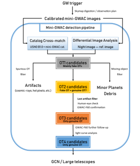
Figure 3: A schematic view of the mini-GWAC detection pipeline for optical transients. Our pipeline identifies the optical transient candidates through different steps using both automatic and human actions.

After our selection process, the transient candidates are classified under six categories in our database:

• Category A / The sources already catalogued: This category groups together the OT candidates that have finally matched the positions of known catalogued stars in the SIMBAD database (Wenger et al., 2000). This database is complete for the limiting magnitude of the mini-GWAC telescopes (V=12).
  

• Category B / The suspected variable/flaring stars: These OT candidates are tagged as variable stars when their positions matched the one of an already catalogued variable star and their lightcurves evolution is in good agreement with the one of the associated variable star.
  

• Category C / The moving objects: The candidates are identified as moving objects by their tracks in several images or if they are already catalogued in the Minor Planet data center.
  

• Category D / The spurious points: This category groups together the OT candidates as being cosmic rays, instrument defects like hot pixels and noise in the residual images. The classification criteria are based on the occurrence rate of the source in our images. Typically, an OT candidate with an occurrence of less than twice in the image time series, its historical data and the residual image is identified as noise.
  

• Category E / The OTs with a host galaxy: This category groups the OT3 candidates that have matched, within a circle region of 90 arcsec around the mini-GWAC position (corresponding to $\sim$3 mini-GWAC pixels), the position of very nearby galaxies of the RC3 catalog (Corwin et al., 1994). This catalog is complete enough at the mini-GWAC limiting magnitude. This category actually may gather kilonovas (for the purpose of GW optical follow-up), supernovae, bright tidal disruption events, etc.
  

• Category F / The host-less OTs: This category groups the OT3 candidates having no match with the RC3 galaxy catalog. Typically, these candidates may correspond to host-less astrophysical events or extragalactic/cosmological events such as Gamma-ray Burst afterglows.

3.3 The detection efficiency of mini-GWAC system

The optical transient search program has run for several years from 2014 to 2017 (not continuously) and being updated every year. In this section, we aim to estimate the number optical transients the mini-GWAC telescopes are able to serendipitously detect in single frames according to our archival data. Our analysis is based on the latest period of mini-GWAC operation when the detection pipeline was upgraded to its last version so that the perfomances could be compared to the period covered by the O2 run. We selected six months of data between Oct. 2016 and Mar. 2017 which corresponds to a total amount of 1673607 images.
Within this period of archival data, 75 individual optical transient sources (typically flaring stars and few unclassified astrophysical optical transients) were detected by mini-GWAC in several hundreds of single frames. We therefore estimate that the expected number of new transients per single frame is on average $\mathrm{N_{OT/frame}=4.5\times 10^{-5}\leavevmode\nobreak\ OT/frame}$. In other words, the mini-GWAC network is able to detect a new optical transient such as flaring stars brighter than $\rm{m_{R}}\sim$ 12 about every 11.5 days assuming that on average a night at Xinglong lasts 8 hours. For a single camera, one night corresponds to about 1920 frames (including the readout time of 5 seconds for each frame). The OTs detected by one mini-GWAC camera can be considered as Poissonian events in our sky survey observations with a typical rate per night given by $\mathrm{\lambda=N_{OT/frame}\times 1920\leavevmode\nobreak\ OT/night}$. As a consequence, we estimate that the Poissonian probability of detecting at least one OT, brighter than $\rm{m_{R}}\sim$ 12, during a night with one camera is $\mathrm{P[N_{OT,night}\geq 1|\lambda=8.6\times 10^{-2}]\sim 8.2\%}$.
A single frame catches a sky pattern of about 400 square degrees which finally gives the number of optical transient per square degree per frame exposure time one may expect to detect by chance with one mini-GWAC camera:

$$\begin{split}\mathrm{N_{OT/sq.deg/\Delta T_{frame}}=\frac{N_{OT/frame}}{FoV_{RA}\times FoV_{dec}}=1.1\times 10^{-7}}\\ \mathrm{\leavevmode\nobreak\ OT\cdot deg^{-2}\cdot\Delta T^{-1}_{frame}}\end{split}$$ (1)

where $\mathrm{\Delta T_{frame}}$ = 10 seconds and $\mathrm{FoV_{RA}=FoV_{dec}=20^{\circ}}$. We emphasize that these statistics have to be taken as rough estimates of the mini-GWAC perfomances since they are averaged on very different observational conditions (weather, sky brightness, moon distance, airmass, duration of the observations per night, etc.) and random source positions in the images for which the detection efficiency can vary between the edge and the inner part of the image, see 3.1. However, these statistics give the right order of magnitude and will be useful to understand the significance of any association of an OT detected in spatial coincidence with a gravitational wave event.

4 The O2 follow-up campaign of mini-GWAC

During the O2 GW observational campaign, 14 alerts have been sent to the external partners of the LIGO/Virgo Collaborations (LVC). The GW candidates were classified into two categories of potential astrophysicals events able to emit gravitational waves: the compact binary mergers including black holes and/or neutron stars on one hand, and the collapse of a massive star or magnetars instabilities (Kotake et al., 2006; Ott, 2009; Gossan et al., 2015; Mereghetti, 2008) (mentionned as Burst) on the other hand.
The alerts with false alarm rates less than one per two months were distributed in the format of notices and circulars via private GCNs. The latency of the initial alert dissemination was ranging from 30 minutes to few hours due to the necessary human validation of the data quality. Regular updates of the localization error box of the candidates were sent by LIGO/Virgo few hours up to few months. All the events were finally classified much later through an offline analysis performed by the LVC (Abbott et al., 2019). All of the confirmed events originated from compact binary mergers and except GW170817, the only BNS merger, they were classified as BBH mergers.

4.1 Alert reception system with mini-GWAC

The GW alerts were received through the GCN system as described in (Abbott et al., 2019) and then recomposed in a VOEvent format. The GW bayesian probability skymaps were decomposed using the predefined mini-GWAC sky grids. A list of tiles were therefore scheduled for observations by order of priority based on their respective probability of containing the GW event. The observation plan was performed for each telescope so that the different tiles can be observed several times during the night.
The recomposed alerts were produced by our french science center located at the Laboratoire de l’Accélérateur Linéaire (LAL) institute in Paris-Orsay and transmitted to the NAOC at Beijing into the chinese science center that operates our telescopes at the Xinglong Observatory. The message transfer connection was built with our own scripts developed in python language based on pub/sub mode of zeroMQ, which has features of authentication, encryption, and validation of the messages. The connection protocol also supports automatic re-connection and re-sending message. The typical latency time is $\sim 0.16$ s. Taking into account the additional delays due to the parsing and the rewriting of the VOEvent alert as well as the response delay of the telescopes, the total latency for the alert receipt by mini-GWAC was typically less than 2 minutes.

4.2 Our observations with mini-GWAC

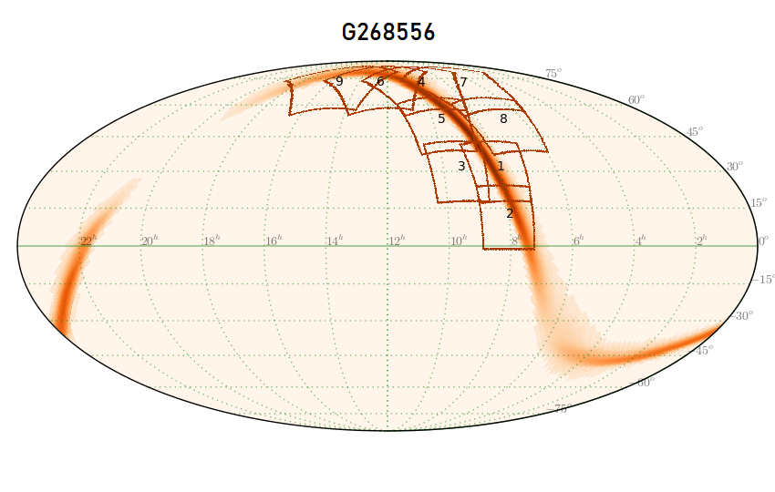
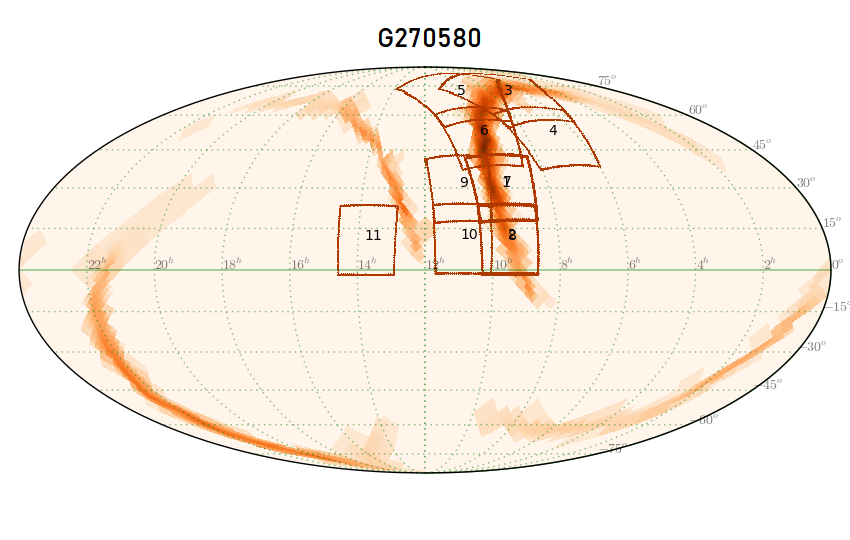
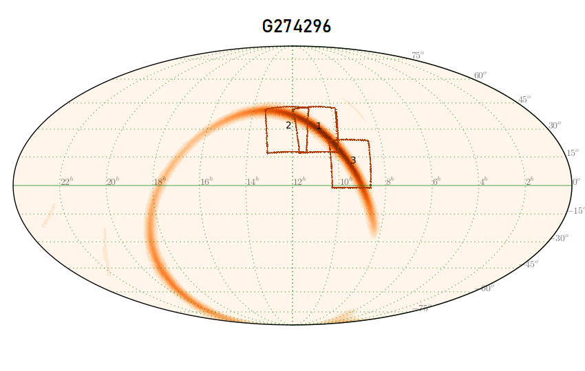
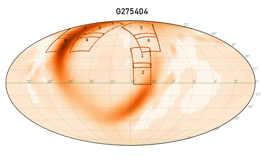
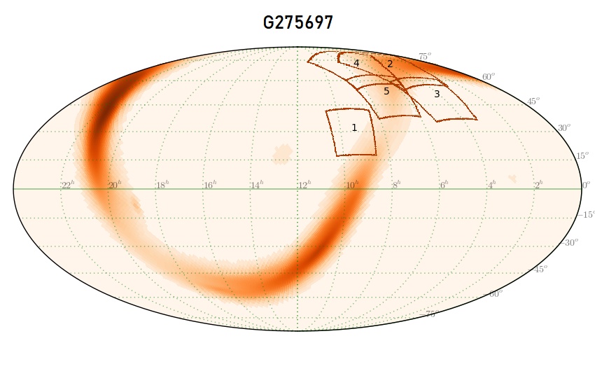
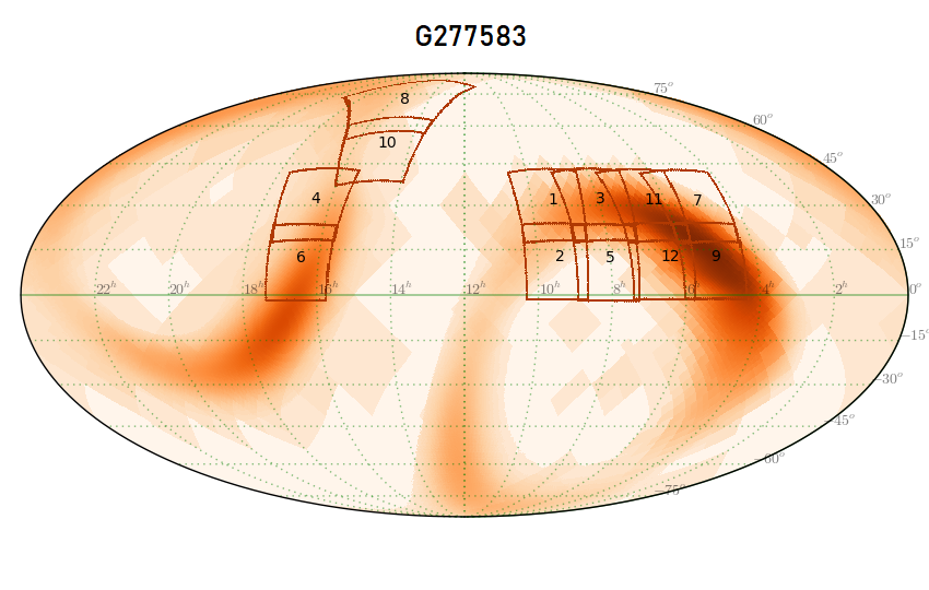
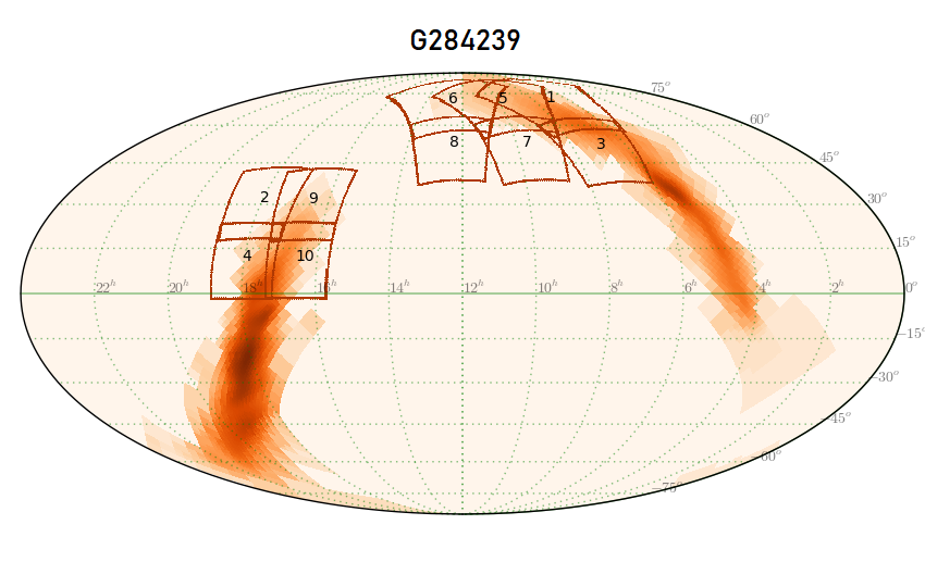
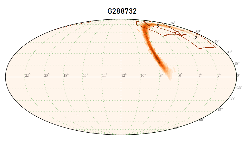
Figure 10: The bayesian probability skymaps of the eight gravitational wave events we followed-up during the O2 run. Our observation grids are shown with the red squares, each of them are identified with a grid ID. All these grids were not necessarily scheduled at the same period because of observational constraints but it shows how we paved the GW error boxes all along our periods of observation.

During the O2 campaign, the mini-GWAC telescopes followed-up 8/14 gravitational waves alerts as shown in Figure 10. The localization regions of the six other GW alerts were not visible at the Xinglong Observatory at all.

From our eight successful follow-ups, two of them (GW170104, GW170608) were confirmed as GW sources originated from the inspiral and the merger of two black holes. The six remaining events were later retracted (Abbott et al., 2019). The main results of our observational campaign are summarized in Table 1.

Table 1: Summary of the observations made at the Xinglong observatory during the O2 GW run with the mini-GWAC telescopes.

Gravitational wave triggers					mini-GWAC observations
ID	Trigger date	Loc. error	confirmed/type		$\leavevmode\nobreak\ \leavevmode\nobreak\ \leavevmode\nobreak\ \leavevmode\nobreak\ \leavevmode\nobreak\ \leavevmode\nobreak\ \leavevmode\nobreak\ \leavevmode\nobreak\ \mathrm{T_{start}}$	$\mathrm{\Delta T_{obs}}$	$\mathrm{P_{GW,cov}}$	NOT2	GCN Reference
	(UTC)	(90%) deg2				(h)	on $\mathrm{\Delta T_{obs}}$	(MP tag)
(1)	(2)	(3)	(4)		(5)	(6)	(7)	(8)	(9)
G268556(1)	2017-01-04 10:11:58	1630	Yes / BBH		$\mathrm{T_{GW}+2.3\leavevmode\nobreak\ h}$	$\sim$10.0	62.4$\%$	273 (2)	Wei et al. 2017a
G270580	2017-01-20 12:30:59.35	3120	No / Burst		$\mathrm{T_{GW}+20\leavevmode\nobreak\ min}$	$\sim$9.5	53.8$\%$	30 (1)	Wei et al. 2017b
G274296	2017-02-17 06:05:55.05	2140	No / Burst		$\mathrm{T_{GW}+6.3\leavevmode\nobreak\ h}$	$\sim$5.0	63.8$\%$	5 (3)	Wei et al. 2017c
G275404	2017-02-25 18:30:21	2100	No / NS-BH		$\mathrm{T_{GW}-5.5\leavevmode\nobreak\ h}$	$\sim$9.0	31.7$\%$	88 (3)	Wei et al. 2017d
G275697	2017-02-27 18:57:31	1820	No / BNS		$\mathrm{T_{GW}+2.7\leavevmode\nobreak\ d}$	$\sim$7.0	6.4$\%$	0	Wei et al. 2017e
G277583	2017-03-13 22:40:09.59	12140	No / Burst		$\mathrm{T_{GW}+12.5\leavevmode\nobreak\ h}$	$\sim$10.0	46.2$\%$	198 (8)	Wei et al. 2017f
G284239	2017-05-02 22:26:07.91	3590	No / Burst		$\mathrm{T_{GW}+2.6\leavevmode\nobreak\ d}$	$\sim$8.0	22.0$\%$	47 (0)	Xin et al. 2017
G288732(2)	2017-06-08 02:01:16.492	860	Yes / BBH		$\mathrm{T_{GW}+15\leavevmode\nobreak\ h}$	$\sim$2.5	18.5$\%$	8 (0)	Leroy et al. 2017

Note: The latency of the first image with the GW trigger time takes into account the GW alert transmission delay by the LVC to the multi-messenger community as well as the delay due to our own system and the local weather conditions. (3) See (Abbott et al., 2019). (6) is the duration of the mini-GWAC observations related to each trigger. (7) is the bayesian probability (integrated over our observation time) that the GW source is in our images based on the final release of the GW Bayestar skymap. (8) is the number of optical transient candidates (OT2) found during $\mathrm{\Delta T_{obs}}$ in the GW sky localization area (90% C.L.). None of these candidates were finally classified as real OT and so be credibly related to any GW event. The numbers of OT candidates identified as minor planets are indicated in parenthesis. ⁽¹⁾ renamed GW170104; ⁽²⁾ renamed GW170608.

4.2.1 Response latencies to the O2 GW alerts

Except for two events (G275697 and G284239) where the weather conditions prevented us from observing as soon as the GW trigger was received, we responded with a short latency to the GW alerts, typically within few minutes after the receipt of the alert messages. We then continuously monitored the sky localization areas during several hours in the first night following the GW trigger times. For half of the followed-up GW alerts (G268556, G270580, G274296 and G275404), we were actually already observing a part of their sky localization areas during our survey program prior to the alert receipt (and even before the GW event for G275404), see Figure 4.

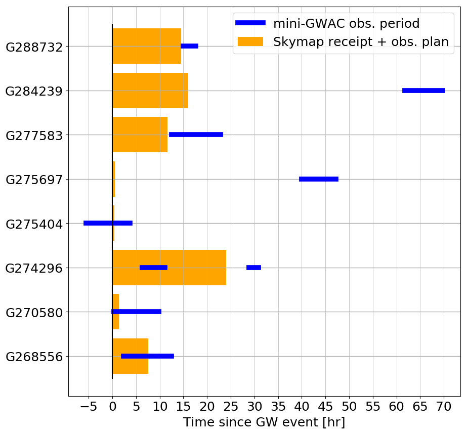
Figure 4: The mini-GWAC response latencies to the GW alerts. For each GW event followed-up by mini-GWAC during O2, the orange bars correspond to the delivery time of the alert at the Xinglong Observatory. This delivery time is mainly due to the time for the LIGO/Virgo Collaboration to send the circular alerts plus the time for our alert system to digest the GW skymap and produce an observation plan for mini-GWAC. The blue bars show the period of our observations with respect to the GW trigger time.

This highlights two major advantages of such wide field of view telescopes observing in survey mode. First, for a significant amount of alerts, they can make simultaneous (even prior for possible precusors) observations based on their regular observational schedule. This also prevents from having no prompt image in case of a failure of the alert receiver system. During our O2 campaign, we experienced two failures of our alert receiver system. For G274296, it had no impact on our follow-up as our mini-GWAC telescopes were actually already monitoring a sky area that covered the full GW error box visible at the Xinglong Observatory. However, for G277583, we underwent an additional delay due to an internet connection loss to start our observations. Once the connection came back, we immediately pointed our mini-GWAC mounts to the GW sky regions.
In a second hand, some images can usually be taken few hours and even days before the GW events in the survey mode, when no electromagnetic counterpart is much expected. Therefore, the wide field of view telescopes have a considerable amount of reference images available for a large fraction of the sky which offers the possibility to make a quick vetting or confirmation of the optical transient candidates that may be found after some merger events by several other facilities.

4.2.2 Coverage of the GW sky localization area

From the GW bayesian probability skymaps, we estimate that the median probability of having the GW events in our images during our periods of observation is 38.9$\%$. For some events, mainly located in the Northern hemisphere, our observations covered more than 60$\%$ of the bayesian localization. This is the largest coverage (based on a GW localization of several thousands of square degrees) performed by any optical telescope on a single night during the O2 campaign. We also computed the real-time performance of our follow-up system concerning the coverage of the bayesian probability skymaps as shown in Figure 5.

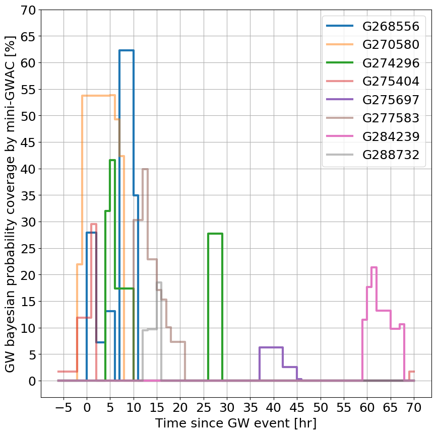
Figure 5: The evolution of our eight GW skymap coverages (bayesian probability) with mini-GWAC as function of time expressed with the delay since the GW trigger time.

During O2, our median instantaneous (based on periods of 1h of observation) bayesian probability coverage of the initial GW alert skymaps was $P_{cov,med}=14.2\%$. This quantity is much more representative of the real capabilities of our mini-GWAC instruments to cover the GW localization area provided by only two interferometers (LIGO Handford and Livingston here). It shows that despite the active participation of the wide field of view telescopes to the follow-up campaign, such as the mini-GWAC telescopes, the need to reduce the GW sky localization area is still crucial to optimise the scientific returns.

4.3 Results

The number of transient candidates found in our images and spatially correlated with the GW events depends on several parameters such as the size of the GW error box and our subsequent coverage of it, the duration of the observations of each grid as well as the local weather conditions (moon brightness, sky transparency, weather status, etc.). Taking these factors into consideration, we ended with more than 200 hundreds OT2 candidates for G268556 while, for example, we could not detect any credible transient source in our follow-up of G275697 (having the poorest coverage of all the GW events of our sample). In Appendix B, we give the details of our observations, grids per grids for each GW event. Our OT2 candidates are detected within a wide range of unfiltered magnitudes (calibrated in R-band Johnson Vega system) $m_{R}\in[12.3-6.8]$ see Figure 6.

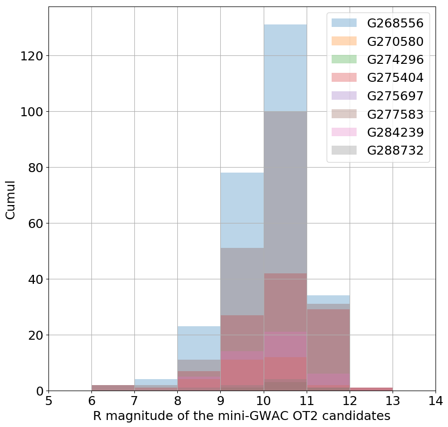
Figure 6: Distribution of the R-band magnitude (unfiltered calibrated with the USNO B1.0 R2mag catalog) of the optical transient (OT2) candidates found in mini-GWAC images for each GW event. These magnitudes are computed at the time of the detection of the OT candidates.

Concerning the two confirmed BBH merger events, GW170104 and GW170608, none of our OT2 candidates (273 and 8, respectively). were classified as real OTs and hence, no OT3 candidates emerged from this step. All of our OT2 candidates were finally classified in the category A (catalogued stars), category C (Minor planets) as shown in Figure 7 or category D (spurious points). As a consequence we could unambiguously reject any association with the two merger events. These null results can be explained both by observational constraints (sensitivity of our telescope, partial coverage of the GW error boxes) and by the physics of the BBH mergers that, if they truly radiate an electromagnetic emission, may power too faint optical transient emissions to be detected by our set of telescopes.

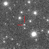
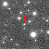
Figure 7: The reference (left) and the first and last night images (middle and right) of a moving object detected by mini-GWAC during our follow-up of G274296 on 2017-02-17 12:18:28 (V = 11.1). Note that this minor planet (471 Papagena) is also present in the reference image (red arrow) a day before with an angular distance of about 13 arcmin with respect to its position measured during our observations.

We compared these null results with the number of optical transients we expected to find spatially correlated with the GW skymaps by chance in our period of observations. To do so, we used the following expression:

$$\begin{split}\mathrm{N^{serendipitous}_{OT,GW}=N_{OT/sq.deg/\Delta T_{frame}}\times f_{GW}\cdot\sigma^{90\%}_{GW}\times N_{frame}}\end{split}$$ (2)

where $\mathrm{N_{OT/sq.deg/\Delta T_{frame}}}$ has been defined in equation 1, $\rm{f_{GW}}$ is the fraction of the GW skymap we covered by our observations, $\mathrm{\sigma^{90\%}_{GW}}$ is the contour of the GW probability skymap given at the 90% confidence level and $\mathrm{N_{frame}}$ is the number of single frames we took during our periods of observation. For each GW event, we actually computed this expression for every single tile covering a portion of the skymap during a certain amount of time, see our observation log in Appendix B. For a given GW event, the final result is the addition of the expectations given in all the individual tiles for those that predict at least one event. Otherwise, if none of the tiles predict any OT detection, we took the best expectation among all the tiles. Concerning our observational campaign of the two BBH merger GW170104 and GW170608 we finally end up with $\mathrm{N^{serendipitous}_{OT,GW}\sim 2.6\times 10^{-2}}$ and $\mathrm{6.0\times 10^{-3}}$ expected OT, respectively. These estimates highlight the fact that any single OT detected in spatial coincident with any of these two GW events would have been of very great interest as a serendipitous OT detection by the mini-GWAC telescopes is strongly unfavored. For completeness we draw the same estimates for all the GW alerts we followed-up and summarize the results in Table 2.

Table 2: Comparison study between the number of OTs we may expect to detect during our follow-up campaign and those we actually detected. For each GW event, no OT has been found in agreement with our expectations. As a consequence, one OT detection would immediately lead to a strong probability of association with the real GW merger events (G268556 and G288732).

GW	$\mathrm{N^{ser.}_{OT,GW}}$ /
event	(OT detected)
G268556	$\mathrm{2.6\times 10^{-2}}$ / (0)
G270580	$\mathrm{1.6\times 10^{-1}}$ / (0)
G274296	$\mathrm{3.5\times 10^{-2}}$ / (0)
G275404	$\mathrm{6.8\times 10^{-3}}$ / (0)
G275697	$\mathrm{7.7\times 10^{-3}}$ / (0)
G277583	$\mathrm{1.5\times 10^{-1}}$ / (0)
G284239	$\mathrm{4.4\times 10^{-2}}$ / (0)
G288732	$\mathrm{2.6\times 10^{-2}}$ / (0)

We tentatively set an upper limit (U.L.) on the optical flux of GW170104 during our period of observations but under the hypothesis that the event was located in the portion of the sky we have monitored. This 3$\sigma$ U.L., lying in the range $m_{R}\in[12.3-11.4]$, varies from a grid to an other one as the sky brightness can significantly change. For GW170608, the limiting magnitude of our images are less stringent because of a cloudy sky. The optical flux upper limit of GW176008 finally lie in the range $m_{R}\in[10.9-9.9]$, again assuming that the event was localized in our images.

5 Towards the next LIGO-Virgo O3 run

The next GW scientific run on April 2019 (O3) promises to be prolific in terms of the number of GW detections that will need extensive electromagnetic follow-up campaigns too. Thanks to the sensitivity improvement of the LIGO-Virgo detectors, one can expect, in the most optimistic scenario, one BNS merger per month and most likely few BBH mergers per week. The localization uncertainties of the GW O3 events will be largely reduced due to the combination of the LIGO-Virgo detectors with a median localization region comprised in the range 120-170 deg² within the 90$\%$ confidence level contours for LIGO only. Despite such significant improvement of the localizations, the need for wide field of view telescopes will be still crucial for some events. Furthermore, according to the expected high GW alert rate, the availability of world-wide networks of telescopes dedicated to the electromagnetic follow-up of the GW events will be a key factor to make the O3 run a scientific success as O2 was.

5.1 From the mini-GWAC to the GWAC system

Since the end of 2017, mini-GWAC have been totally replaced by the nominal design of the GWAC telescopes and are no longer used. Each GWAC mount is equipped with 5 cameras (4 x JFoV camera: 4k x 4k CCD E2V camera with an aperture of 180 mm each + 1 FFoV: 3k x 3k CCD camera with an aperture of 35 mm), see Figure 8. With such a system, each mount will have a field of view of about $25^{\circ}\times 25^{\circ}$ ($\sim$500 square degrees) with an optical flux coverage extended from V $\sim$ 6 magnitude up to 16 magnitude in the visible domain $\mathrm{\lambda\in}$ [500-850 nm]. As for mini-GWAC, an image cadence of 15 seconds is set. For the O3 run, four GWAC mounts will be available at the Xinglong Observatory. We summarize, in Table 3, some parameters of the GWAC telescopes and compare them with those of the mini-GWAC telescopes to highlight the improvements. The major improvements are the increase of the GWAC sensitivity and the angular resolution compared with the mini-GWAC system.

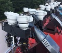
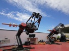
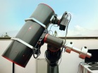
Figure 8: (Left) The GWAC observation system in its test bench at the Xinglong observatory. For O3, it will be composed of 4 mounts. The total FoV of such configuration is about 2000 sq.deg. The imaging time resolution is 15 sec for single frames. (Center) Two GWAC-F60 telescopes (60cm) are used to quickly confirm GWAC optical transients and perform deeper follow-up observations if needed. (Right) A 30 cm telescope (GWAC-F30) will be also used during the O3 campaign (FoV = 1.8${}^{o}\times$ 1.8^o).

Table 3: Comparison between some parameters of mini-GWAC and GWAC.

Parameter	mini-GWAC	GWAC	GWAC
	value	value	improvement factor
Network FoV (sq.deg)	5000	5000	1
Tel. diameter (cm)	7.0	18 (JFOV)	$\sim$ 2.5
Pixel size ($\mu$m)	12	13	$\sim$ 1
Pixel scale (arcsec)	29.5	11.7	2.5
Readout noise (e-)	10	14	0.7
FWHM (center)	1.2	1.5	1.25
$\mathrm{R_{lim}}$ (mag/single frame)	12	16	$\sim$ 40
			(in flux sensitivity)

In association with the GWAC telescopes, our two fully robotized 60 cm telescopes (GWAC-F60A/B) will be also used to automatically confirm the genuineness of the GWAC OT candidates with a localization accuracy of the source of $\sigma\sim 1$ arcsec. They will also provide multi-wavelength (Johnson UBVRI) observations of the galaxies targeted in the GW probability skymaps. Finally, the GWAC system will be completed by the GWAC-F30 robotic telescope (30 cm) operated with a substantial field of view of 1.8${}^{o}\times$ 1.8^o using different filters (Johnson UBVRI). As a whole, this GWAC system offer multiple capabilities of observations and strategies for the optical follow-up of the gravitational wave alerts.

5.1.1 Real-time stacking analysis and search for slow transient

Once data will be taken, we will conduct a stacking analysis of our images to reach a maximum sensitivity of V$\sim$18 (a gain of six magnitude with respect to the mini-GWAC system) in a time-resolution of several hours while keeping a high imaging quality as shown in Figure 9.

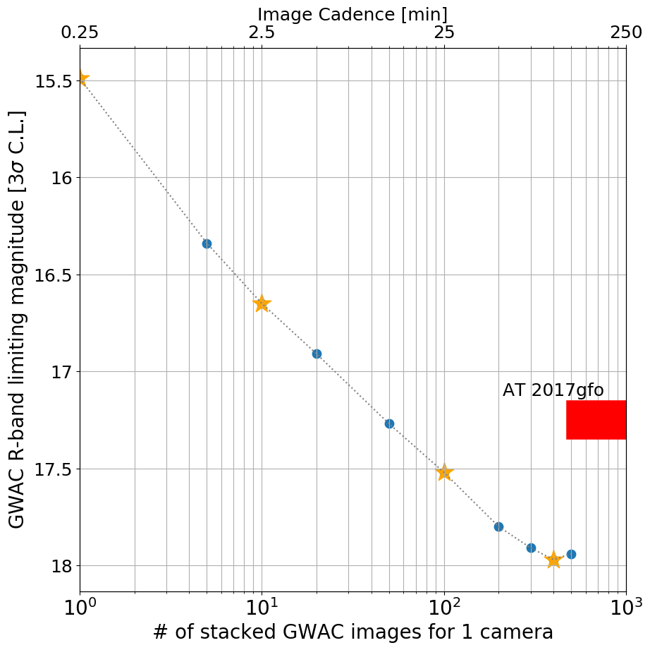
Figure 9: (Top) Series of stacked GWAC sub-images using N = 1 (single image), 10, 100 and 400 images, respectively from left to right. From the left to the right images the limiting magnitude goes from R = 15.49 to R = 17.97 (calibrated with the USNO B1.0 R2mag stars). (Bottom ) Limiting magnitudes of GWAC (3$\sigma$ confidence level) as function of the number of stacked images. The orange stars represent the limiting magnitude of the GWAC images shown above. The kilonova (AT 2017gfo) associated with the GW170817 event is shown assuming a minimum typical timescale of 10 hours for the optical emission. Our stacking analysis would allow us to reach the detection threshold for such kind of event.

This kind of set-up is built to search for moderately slow fading and faint transients having low signal-to-noise ratios in our single images. The stacking analysis of GWAC images would permit to reach the detection threshold of the kilonova optical emisison near its maximum brightness if such events are as close and bright as AT 2017gfo, the kilonova optical counterpart of the BNS merger GW 170817, (m${}_{R,peak}\sim 17.2$). The discovery potential of GRB optical afterglow emission is also highly enhanced with such increase of our sensitivity. However, in the case of the GRB afterglows, the geometry of the emission can significantly affect our detection capability, whether the electromagnetic emission is isotropically radiated or through a narrow jet. If a jet is involved, its viewing angle will also play a significant role. If it is seen largely off-axis compared to our line of sight, the electromagnetic flux we may receive will be strongly reduced and delayed, hence disfavoring an optical detection by our telescopes. On the contrary, for a jetted emission seen on-axis at the BNS distance range of LIGO-Virgo for O3 (120Mpc - 60Mpc), we will very likely detect the optical emission that is expected to be significantly brighter than the GWAC sensitivity (R = 16 mag) at early time post merger.

5.1.2 Automatic and quick classification of the transient candidates

A key challenge of the wide field of view telescopes is to be able to quickly identify and classify the numerous transient sources they detect each night. Despite the field of view of the mini-GWAC telescopes was very large, their limiting sensitivities prevented them from detecting a huge number of optical transients every night (few dozens of OT candidates per mount). Therefore, it was still possible to fully involved humans in the loop of the source classification. For GWAC, it will be no longer the case as the sensitivity of each mount is significantly increased and especially considering the real-time stacking analysis. Typically, in one dark night, the GWAC detection pipeline can be triggered (at the very basic level of OT1) hundreds of times using only single images and the cameras of one mount. As explained in 3.1, the preliminary sample of OT candidates is usually composed of artifacts and possibly few genuine astrophysical sources. A new method of OT classification has been developed in the frame work of the GWAC data processing pipeline based on a machine learning approach. This new classification method, that will be described in detail in a separate paper, will use Convolutional Neural Networks (CNN). This approach is now widely used for telescopes having wide field of views (e.g. Gieseke et al., 2017; Sánchez et al., 2018; Mahabal et al., 2019; Jia et al., 2019) and is particularly efficient in detecting bogus in images such as cosmic-rays, hot pixels, etc. (the category D of our own classification ranking, see 3.2) which constitute the major fraction of our false detections at the OT1 level. The goal is to filter out around 95% of the false positives detected in our OT1 candidate sample. It is crucial for such telescopes in order to be efficient in detecting "the good ones" and to ensure that our optical transient candidates will be of a great interest for the astronomical community when we will release public GWAC alerts.

5.1.3 The first training of the SVOM ground follow-up system.

In 2021, the SVOM mission will be endowed with a network of ground optical/NIR telescopes devoted to the follow-up of the SVOM triggers or ToO triggers approved by the SVOM Collaboration (Wei et al., 2016). At completion, this ground segment should be composed of the SVOM/COLIBRI telescope located at the Observatory of San Pedro Mártir (Mexico), a set of ten GWAC mounts located out of China (the location is still under discussion) and some telescopes located in China: ten GWAC mounts, two GWAC-F60, one GWAC-F30 and the C-GFT telescope (1.2m). For the O3 run, only the chinese part of the SVOM segment will be available with four operational GWAC telescopes and also including the C-GFT telescope. The goal of this chinese network is to pave the GW skymap in the most efficient way by combining different observational strategies such as tiling observations of the GW skymap or galaxy targeting. This strategies will take into account the individual characteristics of our telescopes that will be connected to the SVOM chinese science center (CSC) for O3 at the National Astronomical Observatories of China (NAOC), CAS. The CSC will be in charge of collecting all the observational results and producing the public reports. This centralized database system will allow us to adapt our strategy almost in real time depending whether we need to explore new fields, make some revisit observations or confirm optical transient candidates with multi-band photometric observations. With such system, we will provide, as fast as possible and publicly through the GCN network, the list of the most interesting OT candidates we have found: the so-called OT4 candidates according to our internal labeling system described above. In order to better characterize these promising OTs, based on their temporal behavior and their color evolution, we will conduct spectroscopic follow-up observations using the 2.16m telescope at the Xinglong Observatory and the 2.4m telescope at the Lijiang station of the Yunnan Observatory. Note that we can also perform deep color photometry with such telescopes with a limiting magnitude B/V/R $\sim$ 22 for 10 minute exposure time (under an airmass = 1.3) with the BFOSC instrument mounted on the 2.16m telescope (Fan et al., 2016). For the same exposure time, we can reach a R $\sim 24$ limiting magnitude with the 2.4 m telescopes. During the O2 run, we performed such deep follow-up observations with the 2.16m telescope at Xinglong for an optical transient detected by Swift/UVOT related to the GW trigger G299232 (Meng et al., 2017). We could not detect this transient down to a magnitude r $\sim$ 22 confirming its fading behavior compared to the Swift/UVOT data and consistent with observations performed by other teams. This example shows how these moderately large telescopes will allow us to extend our follow-up capabilities for faint sources (r $<22$) to possibly detect sources similar to the GW170817/AT 2017gfo kilonova (Villar et al., 2017) days after the merger event.

6 Conclusion and Perspectives

The O2 GW observational campaign has opened a new window to study the extreme objects in the Universe. It helped us to validate the capability of the mini-GWAC telescope network as being a fast follow-up system dedicated to the multi-messenger astronomy. So far, our O2 observation campaign represents the largest coverage of the GW sky localization areas made by optical telescopes in short latencies. No credible optical transient was found in our images which we attribute to two main reasons. First, the confirmed GW events we have followed-up, were all originating from BBH mergers from which an electromagnetic emission is highly uncertain. Secondly, the sensitivity of the mini-GWAC telescopes ($m_{R}=12$) was too low to detect faint transient sources such as the kilonova emission like the one observed for GW170817/AT2017gfo or any GRB afterglow emission. Based on this experience, we have presented our new plan for the upcoming O3 run. We showed that the improvement of our observational capabilities by combining both a migration from the mini-GWAC to the GWAC system, with a much higher sensitivity in the visible domain, and the extension of our network will permit us to be more competitive in our searches for optical counterparts from GW events, especially those emerging from the BNS mergers. The O3 run will be also a unique opportunity to build the first blocks of the ground follow-up system of the future SVOM mission that embedded the GWAC system.

Appendices

Appendix A The mini-GWAC follow-up observations of eight O2 GW alerts.

Appendix B The Log. tables of the mini-GWAC observation performed for eight GW events during the O2 LIGO/Virgo run.

Table 4: The observation logs of the mini-GWAC follow-up of G268556 (trig. date: 2017-01-04 10:11:58).

mini-GWAC	$\mathrm{T_{start}}$	$\mathrm{T_{end}}$	mid time	center RA	center dec	$\mathrm{P_{GW,cov}}$	$\mathrm{N_{im}}$ / $\mathrm{N_{OT2}}$	$\mathrm{M_{R,OT2}}$
grid / cam ID	2017-01-04	2017-01-04	(hour)	(h:m:s)	(deg:m:s)			[min - max]
1 / C1	12:30:41.1	13:49:41.5	$\mathrm{T_{GW}+2.9704}$	07:46:49.578	+29:35:33.46	18.5$\%$	316 / 50	[12.3 - 8.7]
2 / C2	12:30:41.1	13:49:49.5	$\mathrm{T_{GW}+2.9715}$	07:48:54.239	+10:34:56.09	13.4$\%$	317 / 36	[11.9 - 8.2]
3 / C1	13:50:29.3	15:14:52.1	$\mathrm{T_{GW}+4.3452}$	09:10:51.599	+29:36:54.60	3.1$\%$	338 / 0	–
7 / C5	14:55:58.2	17:57:22.7	$\mathrm{T_{GW}+6.2451}$	06:34:42.357	+69:28:01.79	3.9$\%$	726 / 0	–
8 / C6	14:56:10.4	17:57:35.7	$\mathrm{T_{GW}+6.2486}$	06:40:16.529	+50:28:28.89	0.3$\%$	726 / 0	–
6 / C3	16:21:28.7	17:57:31.9	$\mathrm{T_{GW}+6.9590}$	11:52:01.006	+70:06:03.83	11.0$\%$	384 / 0	–
4 / C1	19:14:27.3	22:39:37.7	$\mathrm{T_{GW}+10.7513}$	09:17:21.644	+69:37:03.40	17.7$\%$	821 / 142	[11.4 - 6.8]
5 / C2	19:14:27.3	22:39:25.3	$\mathrm{T_{GW}+10.7495}$	09:21:25.794	+50:35:59.26	16.7$\%$	820 / 1	9.9
6 / C5	19:14:32.9	22:39:31.9	$\mathrm{T_{GW}+10.7512}$	11:52:01.006	+70:06:03.83	11.0$\%$	820 / 159	[11.4 - 6.8]
1 / C3	19:14:39.9	21:17:22.8	$\mathrm{T_{GW}+10.0676}$	07:46:49.578	+29:35:33.46	18.5$\%$	490 / 2	[11.1 - 10.5]
2 / C4	19:14:39.9	21:17:36.8	$\mathrm{T_{GW}+10.0695}$	07:48:54.239	+10:34:56.09	13.4$\%$	492 / 24	[11.1 - 8.3]
9 / C7	19:14:55.3	22:39:18.3	$\mathrm{T_{GW}+10.7524}$	14:34:10.239	+70:01:52.84	7.1$\%$	818 / 110	[11.4 - 6.8]

Note: The time of each observation is given in UTC. $\mathrm{T_{start}}$ and $\mathrm{T_{end}}$ correspond to the interval time during which the mini-GWAC telescopes were taking images (with a cadence of 15s). The mid time of the whole mini-GWAC observations is computed in the interval [$\mathrm{T_{start}}-\mathrm{T_{end}}$]. The RA and dec coordinates of the images stand for the center of each image (FoV $\sim 20^{\circ}\times 40^{\circ}$). The number of images as well as the number of optical transient candidates detected during the whole observation period are given for information with $\mathrm{N_{im}}$ and $\mathrm{N_{OT2}}$, respectively. Note that several OT candidates might be detected by different cameras as there are significant overlaps between the observed fields. Finally, $\mathrm{M_{R,OT2}}$ corresponds to the range of magnitudes where the OT candidates were found in single images (unfiltered calibrated with R/Johnson).

Table 5: The observation logs of the mini-GWAC follow-up of G270580 ( trig. date: 2017-01-20 12:30:59.35). Same caption as for table 4.

mini-GWAC	$\mathrm{T_{start}}$	$\mathrm{T_{end}}$	mid time	center RA	center dec	$\mathrm{P_{GW,cov}}$	$\mathrm{N_{im}}$ / $\mathrm{N_{OT2}}$	$\mathrm{M_{R,OT2}}$
grid / cam ID	2017-01-20	2017-01-20	(hour)	(h:m:s)	(deg:m:s)			[min - max]
1 / C1	12:50:28.3	14:15:07.6	$\mathrm{T_{GW}+1.0302}$	09:10:23.301	+29:35:57.71	16.2$\%$	339 / 1	8.6
2 / C2	12:50:28.3	22:14:58.6	$\mathrm{T_{GW}+5.0289}$	09:12:26.259	+10:35:26.10	8.3$\%$	2258 / 0	–
3 / C5	13:50:51.4	19:47:59.1	$\mathrm{T_{GW}+4.3072}$	06:36:32.060	+69:30:22.27	12.7$\%$	1429 / 20	[11.7 - 9.6]
4 / C6	13:50:51.4	19:48:01.2	$\mathrm{T_{GW}+4.3072}$	06:42:03.137	+50:31:15.23	0.2$\%$	1429 / 0	–
5 / C1	14:15:35.4	22:19:45.5	$\mathrm{T_{GW}+5.7781}$	09:17:48.639	+69:36:41.75	12.9$\%$	1937 / 6	[11.8 - 10.2]
6 / C2	14:15:35.4	22:19:48.5	$\mathrm{T_{GW}+5.7785}$	09:21:16.884	+50:34:54.73	23.0$\%$	1937 / 2	[10.3 - 10.2]
1 / C3	14:16:01.4	21:24:39.2	$\mathrm{T_{GW}+5.3224}$	09:08:57.610	+30:01:54.06	16.4$\%$	1715 / 4	[11.8 - 8.4]
2 / C4	14:16:01.4	21:25:03.9	$\mathrm{T_{GW}+5.3259}$	09:13:11.448	+09:57:30.75	8.0$\%$	1716 / 3	[11.5 - 11.1]
9 / C5	19:49:04.7	21:36:13.2	$\mathrm{T_{GW}+8.1943}$	10:34:34.322	+29:30:16.35	5.3$\%$	429 / 1	8.4
10 / C6	19:49:27.9	22:19:41.5	$\mathrm{T_{GW}+8.5598}$	10:37:18.165	+10:30:56.78	0.1$\%$	601 / 0	–
11 / C4	21:32:19.1	22:19:53.1	$\mathrm{T_{GW}+9.4185}$	13:29:12.042	+10:00:17.26	0.1$\%$	190 / 0	–

Table 6: The observation logs of the mini-GWAC follow-up of G274296 ( trig. date: 2017-02-17 06:05:55.05). Same caption as for table 4. ^† For this set of observations the corresponding date is 2017-02-18.

mini-GWAC	$\mathrm{T_{start}}$	$\mathrm{T_{end}}$	mid time	center RA	center dec	$\mathrm{P_{GW,cov}}$	$\mathrm{N_{im}}$ / $\mathrm{N_{OT2}}$	$\mathrm{M_{R,OT2}}$
grid / cam ID	2017-02-17	2017-02-17	(hour)	(h:m:s)	(deg:m:s)			[min - max]
1 / C1	12:20:29.0	13:45:04.7	$\mathrm{T_{GW}+6.1144}$	10:34:48.326	+29:29:08.60	32.0$\%$	338 / 4	[12.2 - 8.5]
2 / C1	13:45:30.2	17:12:33.6	$\mathrm{T_{GW}+8.5519}$	11:58:53.431	+29:29:28.69	17.4$\%$	828 / 1	9.6
3 / C6†	10:53:52.3	12:57:00.8	$\mathrm{T_{GW}+28.9920}$	09:12:10.933	+10:39:50.19	27.7$\%$	493 / 0	–

Table 7: The observation logs of the mini-GWAC follow-up of G275404 ( trig. date: 2017-02-25 18:30:21). Same caption as for table 4.

mini-GWAC	$\mathrm{T_{start}}$	$\mathrm{T_{end}}$	mid time	center RA	center dec	$\mathrm{P_{GW,cov}}$	$\mathrm{N_{im}}$ / $\mathrm{N_{OT2}}$	$\mathrm{M_{R,OT2}}$
grid / cam ID	2017-02-25	2017-02-25	(hour)	(h:m:s)	(deg:m:s)			[min - max]
5 / C7	13:01:04.2	21:37:38.1	$\mathrm{T_{GW}-1.1832}$	09:21:25.5	+69:40:01	1.4$\%$	2066 / 0	–
6 / C8	13:01:04.2	21:37:39.7	$\mathrm{T_{GW}-1.1831}$	09:23:01.6	+50:00:25	0.4$\%$	2066 / 1	12.0
1 / C3	19:23:51.9	20:41:04.7	$\mathrm{T_{GW}+1.5354}$	10:33:59.6	+30:12:22	0.5$\%$	309 / 2	[11.6 - 9.2]
2 / C4	19:23:51.9	20:41:06.2	$\mathrm{T_{GW}+1.5356}$	10:38:05.6	+10:07:57	1.8$\%$	309 / 50	[12.1 - 5.3]
3 / C5	19:23:42.2	22:13:19.6	$\mathrm{T_{GW}+2.3027}$	17:18:04.0	+69:28:00	6.9$\%$	678 / 32	[12.2 - 10.4]
4 / C6	19:23:44.7	22:13:38.0	$\mathrm{T_{GW}+2.3057}$	17:21:47.1	+50:28:32	2.0$\%$	680 / 4	[11.9 - 11.8]
7 / C7	21:39:38.3	22:13:28.5	$\mathrm{T_{GW}+3.4368}$	20:00:36.6	+69:38:42	12.5$\%$	135 / 0	–
8 / C8	21:39:38.3	22:13:25.5	$\mathrm{T_{GW}+3.4364}$	20:01:12.7	+50:00:21	16.4$\%$	135 / 0	–

Table 8: The observation logs of the mini-GWAC follow-up of G275697 ( trig. date: 2017-02-27 18:57:31). Same caption as for table 4.

mini-GWAC	$\mathrm{T_{start}}$	$\mathrm{T_{end}}$	mid time	center RA	center dec	$\mathrm{P_{GW,cov}}$	$\mathrm{N_{im}}$ / $\mathrm{N_{OT2}}$	$\mathrm{M_{R,OT2}}$
grid / cam ID	2017-03-01	2017-03-01	(hour)	(h:m:s)	(deg:m:s)			[min - max]
1 / C1	10:55:43.4	18:11:04.6	$\mathrm{T_{GW}+43.5981}$	09:10:04.5	+29:30:47	0.3$\%$	1741 / 0	–
2 / C3	10:55:26.9	14:04:55.7	$\mathrm{T_{GW}+41.5445}$	03:52:34.0	+68:53:23	5.0$\%$	758 / 0	–
3 / C4	10:55:26.9	14:04:55.7	$\mathrm{T_{GW}+41.5445}$	04:02:12.2	+48:48:08	0.4$\%$	758 / 0	–
4 / C5	10:55:24.5	17:44:07.8	$\mathrm{T_{GW}+43.3709}$	06:34:55.5	+69:32:01	1.5$\%$	1635 / 0	–
5 / C6	10:55:24.5	17:44:07.8	$\mathrm{T_{GW}+43.3709}$	06:40:15.5	+50:32:35	1.3$\%$	1635 / 0	–

Table 9: The observation logs of the mini-GWAC follow-up of G277583 ( trig. date: 2017-03-13 22:40:09.59). Same caption as for table 4.

mini-GWAC	$\mathrm{T_{start}}$	$\mathrm{T_{end}}$	mid time	center RA	center dec	$\mathrm{P_{GW,cov}}$	$\mathrm{N_{im}}$ / $\mathrm{N_{OT2}}$	$\mathrm{M_{R,OT2}}$
grid / cam ID	2017-03-14	2017-03-14	(hour)	(h:m:s)	(deg:m:s)			[min - max]
9 / C6	11:10:11	13:33:39	$\mathrm{T_{GW}+13.6959}$	04:58:00.5	+10:28:12	19.2$\%$	574 / 35	[11.5 - 7.6]
1 / C1	11:10:29	17:59:02	$\mathrm{T_{GW}+15.9100}$	09:10:29.8	+29:50:17	2.4$\%$	1634 / 18	[12.2 - 9.1]
7 / C5	11:10:30	13:33:01	$\mathrm{T_{GW}+13.6933}$	04:55:10.8	+29:25:59	7.3$\%$	570 / 41	[11.7 - 8.9]
3 / C3	11:10:45	16:40:29	$\mathrm{T_{GW}+15.2576}$	07:46:15.6	+29:57:47	6.2$\%$	1319 / 16	[12.0 - 6.8]
5 / C4	11:10:45	16:40:01	$\mathrm{T_{GW}+15.2537}$	07:50:25.4	+09:54:53	1.1$\%$	1317 / 9	[11.8 - 9.8]
2 / C2	11:10:55	17:59:54	$\mathrm{T_{GW}+15.9208}$	09:13:10.6	+10:17:08	1.0$\%$	1635 / 4	[11.4 - 9.9]
12 / C8	12:45:01	15:56:16	$\mathrm{T_{GW}+15.6747}$	06:20:02.3	+10:21:24	8.2$\%$	765 / 52	[11.8 - 9.3]
11 / C7	12:45:41	14:56:37	$\mathrm{T_{GW}+15.1832}$	06:18:37.7	+29:46:06	11.5$\%$	524 / 22	[11.6 - 8.9]
10 / C6	13:34:09	21:30:00	$\mathrm{T_{GW}+18.8653}$	14:40:07.7	+50:29:58	0.4$\%$	1903 / 0	–
8 / C5	13:34:31	21:30:00	$\mathrm{T_{GW}+18.8683}$	14:36:21.1	+69:30:06	0.8$\%$	1902 / 1	10.7
6 / C4	16:50:38	21:30:00	$\mathrm{T_{GW}+20.5026}$	16:18:18.2	+09:59:04	5.3$\%$	1117 / 0	–
4 / C3	16:50:46	21:30:00	$\mathrm{T_{GW}+20.5037}$	16:14:18.2	+30:03:36	1.5$\%$	1117 / 0	–

Table 10: The observation logs of the mini-GWAC follow-up of G284239 ( trig. date: 2017-05-02 22:26:07.91). Same caption as for table 4.

mini-GWAC	$\mathrm{T_{start}}$	$\mathrm{T_{end}}$	mid time	center RA	center dec	$\mathrm{P_{GW,cov}}$	$\mathrm{N_{im}}$ / $\mathrm{N_{OT2}}$	$\mathrm{M_{R,OT2}}$
grid / cam ID	2017-05-05	2017-05-05	(hour)	(h:m:s)	(deg:m:s)
5 / C5	12:10:29	17:09:26	$\mathrm{T_{GW}+64.2304}$	09:15:43.9	+69:29:34	3.2$\%$	1196 / 0	–
7 / C6	12:10:29	17:09:36	$\mathrm{T_{GW}+64.2318}$	09:21:17.0	+50:29:41	0.7$\%$	1196 / 0	–
9 / C7	12:11:12	20:09:24	$\mathrm{T_{GW}+65.7361}$	16:15:56.4	+29:39:59	1.7$\%$	1913 / 0	–
3 / C4	12:15:52	14:07:41	$\mathrm{T_{GW}+62.7607}$	06:44:38.4	+49:45:43	6.9$\%$	447 / 0	–
1 / C3	12:18:07	14:09:34	$\mathrm{T_{GW}+62.7952}$	06:35:33.2	+70:03:11	6.1$\%$	446 / 0	–
10 / C8	12:45:41	20:09:30	$\mathrm{T_{GW}+66.0243}$	16:16:57.1	+10:13:56	6.2$\%$	1775 / 30	[11.8 - 10.3]
4 / C4	14:15:38	20:09:05	$\mathrm{T_{GW}+66.7704}$	17:45:33.4	+10:00:59	5.2$\%$	447 / 17	[11.8 - 9.9]
2 / C3	14:17:02	20:09:33	$\mathrm{T_{GW}+66.7860}$	17:41:40.8	+30:05:48	0.3$\%$	1410 / 0	–
8 / C6	17:10:50	20:04:52	$\mathrm{T_{GW}+68.1953}$	12:01:27.8	+50:23:40	$<0.1\%$	696 / 0	–
6 / C5	19:59:14	20:09:17	$\mathrm{T_{GW}+69.6354}$	11:56:29.8	+69:27:40	0.8$\%$	40 / 0	–

Table 11: The observation logs of the mini-GWAC follow-up of G288732 ( trig. date: 2017-06-08 02:01:16.492). Same caption as for table 4.

mini-GWAC	$\mathrm{T_{start}}$	$\mathrm{T_{end}}$	mid time	center RA	center dec	$\mathrm{P_{GW,cov}}$	$\mathrm{N_{im}}$ / $\mathrm{N_{OT2}}$	$\mathrm{M_{R,OT2}}$
grid / cam ID	2017-06-08	2017-06-08	(hour)	(h:m:s)	(deg:m:s)			[min - max]
1 / C3	16:58:35	19:36:46	$\mathrm{T_{GW}+16.2733}$	01:15:34.8	+70:03:21	9.5$\%$	633 / 4	[9.9 - 8.8]
2 / C4	17:10:44	19:31:01	$\mathrm{T_{GW}+16.3267}$	01:22:21.1	+49:56:18	0.5$\%$	561 / 0	–
3 / C5	19:10:51	19:32:59	$\mathrm{T_{GW}+17.3440}$	03:56:21.7	+69:30:35	16.4$\%$	89 / 4	[10.9 - 9.8]

References

- Abbott et al. (2016a) Abbott, B. P., Abbott, R., Abbott, T. D., et al., 2016a, PRL, 116, 241102
- Abbott et al. (2016b) Abbott, B. P., Abbott, R., Abbott, T. D., et al., 2016b, PRL, 116, 061102
- Abbott et al. (2016c) Abbott, B. P., Abbott, R., Abbott, T. D., et al., 2016c, PRL, 116, 241103
- Abbott et al. (2017a) Abbott, B. P., Abbott, R., Abbott, T. D., et al., 2017a, PRL, 119, 161101
- Abbott et al. (2017b) Abbott, B. P., Abbott, R., Abbott, T. D., et al., 2017b, ApJL, 848, L12
- Abbott et al. (2017c) Abbott, B. P., Abbott, R., Abbott, T. D., et al., 2017c, ApJL, 848, L13
- Abbott et al. (2017d) Abbott, B. P., Abbott, R., Abbott, T. D., et al., 2017d, PRL, 119, 141101
- Abbott et al. (2019) The LIGO Scientific Collaboration and the Virgo Collaboration, 2019, arXiv e-prints, arXiv:1901.03310
- Alard (2000) Alard, C. 2000, A&AS, 144, 363
- Berger (2014) Berger, E., 2014, ARAA, 52, 43-105
- Bertin & Arnouts (1996) Bertin, E. & Arnouts, S., 1996, A&AS, v.117, p.393-404
- Corwin et al. (1994) Corwin, Jr., H. G., Buta, R. J. and de Vaucouleurs, G., 1994, AJ, 108, 2128-2144
- Eichler et al. (1989) Eichler, D., Livio, M., Piran T. & Schramm D. N., 1989, Nature, 340, 126-128
- Fan et al. (2016) Fan, Z., Wang, H., Jiang, X., Wu, H., et al., 2016, PASP, 128, 11
- Gieseke et al. (2017) Gieseke, F., Bloemen, S., van den Bogaard C. & Heskes T., et al., 2017, MNRAS, 472, 3101-3114
- Goldstein et al. (2017) Goldstein, A., Veres, P., Burns, E., Briggs, M. S., et al., 2017, ApJ, 848, L14
- Gossan et al. (2015) Gossan, S., Ott, C., Kalmus, P. & Sutton, P., 2015, APS April Meeting Abstracts, C7.002
- Huang et al. (2015) Huang, L., Xin, L. P., Han X. H. & Wei J. Y., 2015, Optics and Precision Engineering, 23, 174
- Jia et al. (2019) Jia, P., Zhao, Y. F., Xue, G. & Cai, D. M., 2019, ArXiv e-print, arXiv:1904.12987
- Kotake et al. (2006) Kotake, K., Sato, K. & Takahashi K., 2006, Reports on Progress in Physics, 69, 971-1143
- Kulkarni (2005) Kulkarni, S. R, 2005, ArXiv Astrophysics e-prints, astro-ph/0510256
- Li & Paczyński (1998) Li, L.X, Paczyński, B., 1998, ApJL, 507, L59-L62
- Loeb (2016) Loeb, A., 2016, ApJL, 819, L21
- Mahabal et al. (2019) Mahabal, A., Rebbapragada, U., Walters, R. & Masci, F. J., et al., 2019, PASP, 131, 038002
- Meng et al. (2017) Meng, X. M., Xin, L. P., Antier, S., et al.,2017, GRB Coordinates Network, 21762, 1
- Mereghetti (2008) Mereghetti, S., 2008, A&A review, 15, 225-287
- Metzger et al. (2010) Metzger, B. D. and Martínez-Pinedo, G. and Darbha, S., et al., 2010, MNRAS, 406, 2650-2662
- Metzger (2017) Metzger, B. D., 2017, Living Reviews in Relativity, 20, 3
- de Mink & King (2017) de Mink, S. E. and King, A., 2017, ApJL, 839, L7
- Perna et al. (2016) Perna, R. and Lazzati, D. and Giacomazzo, B., 2016, ApJL, 821, L18
- Ott (2009) Ott, C. D, 2009, Classical and Quantum Gravity, 26, 063001
- Paczyński (1986) Paczyński, B., 1986, ApJL, 308, L43-L46
- Paczyński (1991) Paczyński, B., 1991, Acta Astronomica, 41, 257-267
- Sánchez et al. (2018) Sánchez, B., Domínguez R., M. J., Lares, M. & Beroiz, M., et al., 2018, ArXiv e-print, arXiv:1812.10518
- Wei et al. (2015) Wei, J. Y., Wu, C., Leroy, N., et al., 2015, GRB Coordinates Network, 18763, 1
- Wei et al. (2017a) Wei, J. Y., Han, X. H, Leroy, N., et al., 2017a, GRB Coordinates Network, 20369, 1
- Wei et al. (2017b) Wei, J. Y., Han, X. H, Leroy, N., et al., 2017b, GRB Coordinates Network, 20490, 1
- Wei et al. (2017c) Wei, J. Y., Han, X. H, Wu, C., et al., 2017c, GRB Coordinates Network, 20695, 1
- Wei et al. (2017d) Wei, J. Y., Han, X. H., Meng, X. M., et al., 2017d, GRB Coordinates Network, 20745, 1
- Wei et al. (2017e) Wei, J. Y., Han, X. H., Wang, J., et al., 2017e, GRB Coordinates Network, 20793, 1
- Wei et al. (2017f) Wei, J. Y., Han, X. H., Wu, C., et al., 2017f, GRB Coordinates Network, 20870, 1
- Xin et al. (2017) Xin, L. P., Wei, J. Y., Han, X. H., et al., 2017, GRB Coordinates Network, 21073, 1
- Leroy et al. (2017) Leroy, N., Han, X. H., Antier, S., et al., 2017, GRB Coordinates Network, 21229, 1
- Wei et al. (2016) Wei, J. Y., Cordier, B., Antier, S., et al., 2016, ArXiv e-prints, arXiv:1610.06892
- Villar et al. (2017) Villar, V.A., Guillochon, J., Berger, E., et al., 2017, ApJ, 851, L21
- Wenger et al. (2000) Wenger, M., Ochsenbein, F., Egret, D., et al., 2000, A&AS, 143, 9
- Yang et al. (2019) Yang, X., Liping, X. L., Wei, J. Y, Han, X. H, et al., 2019, in preparation
- Zacharias et al. (2013) Zacharias, N., Finch, C.T., Girard, T.M., et al., 2013, AJ, 145, 44
- Zhang et al. (2016) Zhang, S. N., Liu, Y., Yi, S., et al., 2016, ArXiv e-prints, arXiv:1604.02537
- Zhang (2016) Zhang, B., 2016, ApJ, 827, L31