Computers and turbulence

Abstract

This paper briefly reviews the influence that the rapid evolution of computer power in the last decades has had on turbulence research. It is argued that it can be divided into three stages. In the earliest (‘heroic’) one, simulations were expensive and could at most be considered as substitutes for experiments. Later, as computers grew faster and some meaningful simulations could be performed overnight, it became practical to use them as (‘routine’) tools to provide answers to specific theoretical questions. More recently, some turbulence simulations have become trivial, able to run in minutes, and it is possible to think of computers as ‘Monte Carlo’ theory machines, which can be used to systematically pose a wide range of ‘random’ theoretical questions, only to later evaluate which of them are interesting or useful. Although apparently wasteful, it is argued that this procedure has the advantage of being reasonably independent of received wisdom, and thus more able than human researchers to scape established paradigms. The rate of growth of computer power ensures that the interval between consecutive stages is about fifteen years. Rather than offering conclusions, the purpose of the paper is to stimulate discussion on whether machine- and human-generated theories can be considered comparable concepts, and on how the challenges and opportunities created by our new computer ‘colleagues’ can be made to fit into the traditional research process.

1 Introduction

Although, from its title, this paper may seem to be an appeal for a new and unnecessary journal, it is intended as a review of the role that the rapid development of direct numerical simulations has played over the last decades in the elucidation of turbulence physics, and as a meditation on its possible evolution in the immediate future. It does not address the parallel development of turbulence models and large-eddy simulations, which are the mainstay of industry but which owe less to computational power. As the story unfolds, it should be clear to the reader that many of the themes that we meet in tracing turbulence research can be generalised to the role of computers in other branches of science and technology, some of which have led the way, while others have lagged behind [1, 2, 3, 4]. We may use the former as guides to likely future developments in our field, and the latter as warnings of the pitfalls to be avoided. In addition, and even if a definite answer is well beyond the scope of a paper like the present one, we will briefly discuss what could be the consequences of continuing in the present direction, both for the field and for its practitioners, and leave to the readers the decision on what they think is the right course to follow.

It has become customary to start historical reviews of turbulence with a reference to Leonardo da Vinci. Unfortunately, although he wrote extensively on fluid mechanics and on what later came to be regarded as turbulence, I have been unable to trace any reference to computation or automata applicable to the present review. However, to maintain tradition, I offer a quote which is relevant to the general themes discussed in the paper.

It refers to the relation between theory, experience and data, and can be applied to the hopes of some people, including the author, of what could be expected from computers. It can also be taken as a working definition of a successful theory: “There is nothing in nature without a cause; understand the cause and you will have no need for the experiment” [5, Cod. Atlantico, 147va]. This is clearly a dubious statement, and Leonardo hedges it elsewhere by declaring that: “It is my intention first to cite experience, then to demonstrate through reasoning why experience operates in a given way” [6, Ms E Paris, 55r], or that we should “avoid the teaching of speculators whose judgement is not confirmed by experience” [6, Ms B Paris, 4v]. While aiming for the first of these quotes, this review will try to follow the last two.

The paper is organised in terms of the cost of individual simulations. Section 2 deals with simulations which are very expensive, and §3 discusses the consequences of some simulations becoming inexpensive enough to be considered routine. These two sections can be seen as a short historical survey of the field up to now, but §4 speculates on how turbulence research might be affected when simulations become cheap enough to be deemed trivial, and offers an example. The paper is intended to promote discussion among researchers, and offers no conclusions, but a summary and a list of possible open questions are collected in §5.

2 Turbulence and numerical simulation

Humans must have been aware from very early times that the flow of water is not always smooth, and that crossing a river involves dealing with eddies comparable to the mean drift of the stream. The same applies to the wind, and some of the first recorded uses of the word ‘turbulent’ are applied to the weather. Quantitative study of turbulent flows, even if not recognised as such, must also have been commonplace, because the design of the extensive irrigation canals and aqueducts of antiquity had to rest on a correct estimation of the friction coefficient. Both ancient Greek $(\tau\acute{\upsilon}\rho\beta\eta)$ and Latin (turba–æ) have related words meaning disorder, confusion or turmoil. Several Latin languages still maintain the word turba to describe an unruly mob. Latin has the adjective turbulentus–a, applying to anything disordered or confused, as in turbulent times, weather or sea. The adjective and the verb (turbare), rather than the noun, were kept in use during the Middle Ages. In Spanish, Gonzalo de Berceo (circa 1230) uses them to refer to the weather, to visions and to character. In English, they don’t appear to have been introduced until the XVI century. The Oxford dictionary points to a first use of ‘turbulent’ in the Bible of Coverdale (1538), referring to the “attacks of the wicked”, and to a first reference to ‘turbulent weather’ in the letters of G. Harvey in 1573.

In none of these instances, including those referring to the atmosphere or to the ocean, is there any implication that turbulence is a separate kind of flow. Leonardo da Vinci [5, 6] wrote extensively around 1500 on hydraulic applications and machines, and did detailed sketches and descriptions of the wakes behind objects and of the eddying motions on the surface of pools and rivers. He worried about their effect on bed erosion, and had multiple (mostly incorrect) theories about the origin and effects of eddies, but most hydrodynamics up to the late XIX century was essentially laminar, and dealt with the mean properties of the flow without regard to its fluctuations.

The first recognition of the existence of two different flow regimes probably came around the middle of the XIX century from careful measurements of water friction in pipes. This was at the time a classical problem in practical hydraulics which, together with that of the drag of moving bodies, had been the subject of experimental and theoretical investigations for at least 150 years. It was known that it had two components, one linear and the other approximately quadratic in the fluid velocity, and that only the first one depends on the viscosity of the fluid. Hagen [7] and Poiseuille [8] had inaugurated modern rheology by studying the linear regime in capillaries, and by measuring the dependence of the viscosity on temperature. In 1854 Hagen [9] and Darcy [10] independently published careful measurements on larger pipes and noted that the nonlinear component was dominant, and that it came together with disordered motion in the fluid. Both speculated that the increased drag was due to the energy spent in creating the fluctuating eddies.

Soon after that, Boussinesq [11] published a long paper clearly distinguishing between two different kinds of flow, smooth and ‘tumultuous’. It contained many of the ideas that were later associated with turbulence research, such as a modified eddy viscosity and the realisation that turbulent flows were too complicated for a deterministic description, and had to be treated statistically.

The transition between the two states was clarified in the famous experiments of Reynolds [12], in which he introduced dye at the inlet of a long pipe and observed the process by which the flow became disordered; this is the paper in which he introduced what became known as the ‘Reynolds number’, to describe the circumstances at which the transition took place. In his second important paper on the subject [13] he used for the first time the decomposition of the flow into mean and fluctuating parts, and introduced the concept of Reynolds stresses. It is from this paper that much of the modern statistical theory of turbulence derives. A more complete account of this early period of hydrodynamics can be found in [14].

The first recorded reference to the perturbed flow as turbulent is in the second edition of Lamb [15], who attributes the name to Lord Kelvin and warns that it was, at the time, the “chief outstanding difficulty” of hydrodynamics.

Although some would argue that this warning still applies, the subject has advanced substantially over the intervening century, driven intermittently by improvements in instrumentation and in theory. The 1930’s saw the extension to the study of turbulence of the general flowering of physics, especially that of statistical mechanics, culminating in Kolmogorov’s [16] prediction of the form of the energy spectrum. The following years were dominated by the introduction of the hot wire anemometer, which provided unprecedented amounts of experimental detail on the smaller scales of the flow, joined in the late 1960’s by a renewed interest in optical techniques, which partially shifted the emphasis towards larger coherent eddies.

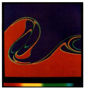
(a)     (b)

Figure 1: (a) Numerical simulation of the roll-up of a vorticity layer. Reproduced with permission from [17]. (b) Laser-induced fluorescent picture of an experimental mixing layer in water. Reproduced with permission from [18].

The first real contribution of computers to turbulence was due to Richardson in the early 1920’s. Up to then, most simulations of turbulence had centred on the mean flow, and on modelling averaged quantities such as drag or mixing efficiency. That was natural, because fluctuations in engineering flows are too fast and too small to be easily observable or relevant. But Richardson was a meteorologist, and the velocity fluctuations in the atmosphere range from weather systems with a lifetime of days and a length scale of the order of a continent, to wind draughts and tornadoes lasting minutes and severely impacting human activity. The mean atmospheric circulation is of great theoretical interest, but its velocity fluctuations are a practical problem.

Besides several seminal contributions to the observation and theory of turbulence, Richardson proposed a way to discretise the equations of weather prediction in terms of centred finite differences [19]. He applied them to an actual simulation of the weather over middle Europe and, although this first experiment did not succeed, his work is now recognised as the foundation of modern prediction schemes [20]. At that time, a computer was a person whose role was to compute, either by hand or with mechanical aids such as a slide rule. Richardson performed his simulation manually while serving at the front during World War I, and he was acutely aware that many more operators would be required to simulate the weather in less than real time. He dedicates the last part of [19] to the ‘coding’ organisation of the work, with a set of forms to be filled by individuals and passed to their neighbours, in an early implementation of parallel multiprocessing and networking. He also estimated the number of workers (64,000) required for a global forecast [21]. He even tried to fund the scheme, but he failed, and meteorological forecasting took a different direction until the advent of electronic computing in the 1950’s.

Not long afterwards, but still before the introduction of electronic computers, Rosenhead [17] presented the numerical simulation of the nonlinear evolution of the Kelvin–Helmholtz instability of a velocity discontinuity. He represented it as a series of point vortices whose motion was traced by a Runge–Kutta scheme, and he was able to describe the formation of the large-scale vortices that later became associated with turbulent shear layers (see figure 1).

Electronic computers began to appear in the 1940’s and became available for scientific research soon afterwards [22]. John von Neumann promoted the design and construction of the first general purpose computers, and organised several groups to exploit them at the Princeton Institute for Advanced Studies [23]. He foresaw that computers would revolutionise the study of nonlinear problems, which were seldom considered at the time for lack of appropriate tools, and identified weather prediction, aerodynamics and turbulence as key areas of application. One of the first weather forecasts resulting from this program is [24], which follows in part the lead of Richardson thirty years before.

The application of computers to the direct simulation of the turbulence fluctuations proceeded quickly after that, mostly driven by the exponential increase in processor speed and memory capacity. The same has been true of experiments, spurred in part by mutual competition with simulations, but it is probably true that, mostly because of their superior observational capabilities, most of the theoretical advances in fundamental turbulence physics now come from simulations.

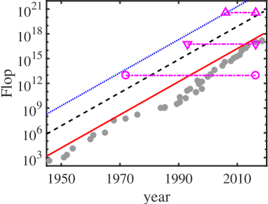
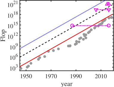
(a)     (b)

Figure 2: (a) The grey closed symbols are the speed of the fastest computer as a function of the year of commission, in floating-point operations (flop) per second. Trend lines are:   , flops per minute;            , overnight;            , three months. They are reduced by a factor of four with respect to nominal values to account for practical inefficiencies [25], and grow by $1000$ every 15 years. The horizontal lines are the number of operations required for simulations of isotropic turbulence, starting at the year of their initial publication: $\circ$, $Re_{\lambda}=35$ [26]; $\scriptscriptstyle\bigtriangledown$, $Re_{\lambda}=150$ [27]; $\scriptstyle\triangle$, $Re_{\lambda}=650$ [28]. (b) As in (a), for turbulent channels: $\circ$, $Re_{\tau}=180$ [29]; $\scriptscriptstyle\bigtriangledown$, $Re_{\tau}=2000$ [30]; $\scriptstyle\triangle$, $Re_{\tau}=5200$ [31].

Estimating when a particular turbulent flow becomes computable depends on the details of the flow and of the code, as well as on economic factors, but some approximate rules can be derived from past experience. Consider the compilations in figure 2. Simulations can be classified as ‘heroic’, lasting for months, ‘routine’, which can be run overnight, and ‘trivial’, which run in a few minutes. The first ones are research projects that are typically performed only once, or at most a few times. The second ones are industrially useful, and although still expensive when measured in terms of researcher’s time, they can be run several times if considered worthy, such as in testing well-developed hypotheses. Trivial simulations can be run many times at little cost, and, as we will discuss below in more detail, may be used to test or propose ideas. The trend lines in figure 2 show that computer speed increases by a factor of 1000 every fifteen years, implying that a heroic job becomes routine in approximately twelve years, and trivial in another twelve.

The cost of turbulence simulations depends primarily on their Reynolds number, which determines the ratio between the largest and the smallest scales, and therefore the number of grid points and operations required. For the simplest case of isotropic turbulence in a triply periodic box, the relevant Reynolds number is $Re_{\lambda}=2K(5/3\varepsilon\nu)^{1/2}$, where $K$ and $\varepsilon$ are, respectively, the kinetic energy and the dissipation per unit volume, and $\nu$ is the kinematic viscosity. It can be shown that the linear range of scales is proportional to $Re_{\lambda}^{3/2}$ [32], so that the number of operations is proportional to $(Re_{\lambda}^{3/2})^{4}=Re_{\lambda}^{6}$ (because there are three spatial dimensions plus time). The first simulation of this flow appeared in 1972 [26], at the marginally turbulent $Re_{\lambda}=35$ in a box of $32^{3}\approx 32,000$ Fourier modes. It is represented in figure 2(a) by the horizontal line with circles starting at the year of its first publication. The other two horizontal lines correspond to later simulations at higher Reynolds number, and it is clear from the figure that each of these simulations was heroic at the time. It is also clear that the first two simulations have by now become trivial, and that the largest one is becoming routine. In fact, $Re_{\lambda}\approx 1000$ is becoming commonplace, and some $Re_{\lambda}\approx 2000$ simulations have been reported at somewhat reduced resolution and shorter evolution times.

More complex flows are more expensive to simulate. Figure 2(b) displays the operation count and publication year for turbulent channels, which are inhomogeneous and anisotropic because of the presence of the wall. The relevant Reynolds number is $Re_{\tau}=u_{\tau}h/\nu\sim Re_{\lambda}^{2}$, where $u_{\tau}$ is the friction velocity and $h$ is the channel half-height. The number of operations scales like $Re_{\tau}^{3}Re_{\tau}^{3/4}=Re_{\tau}^{15/4}$ and, because the anisotropy requires larger computational boxes than the isotropic case, and the numerics are somewhat harder, the first simulation only appeared in 1987 [29], for $Re_{\tau}=180\,(Re_{\lambda}\approx 60)$ using $4\times 10^{6}$ grid points. That case became trivial several years ago. The second simulation in the figure, $Re_{\tau}=2000$, is now routine, but the last one, $Re_{\tau}=5200$, will remain large for some time.

Because the Navier–Stokes equations are generally believed to represent well the motion of fluids, and the theory of numerical approximation is well developed, direct simulations are essentially equivalent to experiments [33]. Some limitations are different in the two cases, but equivalent. For example, the boundary conditions in numerics are equivalent to the details of tripping and of wind tunnel configuration in the laboratory. The question of whether simulations should be pursued at higher Reynolds numbers is thus equivalent to whether experiments should be. The main advantage of the former with respect to the latter is that simulations have less observability limitations. It is essentially impossible to simulate a flow without knowing everything about it. All variables are required to integrate the equations of motion, or can be computed by postprocessing. That is the reason for the high cost of simulations, but it gives them an edge over experiments from the point of view of what can be learned. Even when a high-Reynolds number experiment is performed, what can be measured is usually limited, and the comparison between simulations and experiments should be made at equivalent levels of observability. At present, heroic simulations are probably ahead of experiments in this respect for simple flows, such as the ones mentioned above, and recent results from both simulations [31] and experiments [34] suggest that it is doubtful whether further increasing the Reynolds number would provide more than incremental pay-offs. A rough estimate of the maximum required Reynolds number for channels, based on a separation of scales of two orders of magnitude, is $Re_{\tau}=10^{4}$ [35], and such a simulation is currently under way [36]. For comparison, the Reynolds number of a zero-pressure-gradient boundary layer over the dimensions of a flying bird ($L=0.25$ m, $U=5$ m/s) is $Re_{\tau}\approx 200$, and the one over the fuselage of a medium-sized airliner ($L=25$ m, $U=300$ m/s) is $Re_{\tau}\approx 40000$.

A quick survey of recent large turbulence simulations shows an increase in the number of more complex flows, either from the point of view of geometry [37, 38], or of rheology [39], in detriment of simpler canonical ones.

Two caveats should be mentioned regarding this comparison between simulations and experiments. The first one is that the fuller information from simulations is not always an advantage, because it may not be necessary to know everything about the flow for some particular purpose. If what is required is to answer a specific question, it may be enough to perform an ad-hoc simulation or experiment to answer it, even if other variables are not obtained. These are what we have defined above as ‘routine’ simulations (or experiments), and which technique to choose in each case should be guided by economy and need.

The second caveat is that operation counts may be starting to lose importance as the chief constraint for simulations. Large computations generate huge amounts of data, which, as we will see in the next section, may take a long time to postprocess. Individual flow fields of the largest simulations in figure 2 have file sizes of the order of Terabytes. Minimal statistical significance requires at least 100 such fields, and full advantage of a simulation can only be gained from time-resolved sequences of several thousand files. The resulting multi-Petabyte data sets are not only expensive to store and maintain, but hard to share among interested groups [40, 41], although sharing is one of the main reasons to compile them in the first place. It is becoming increasingly common to process data on the fly [42], without keeping most of them, or to run simulations at full resolution while storing only underesolved data [43]. But doing so detracts from their value. The storage and sharing problem is not restricted to simulations. It is related to the range of scales in high-Reynolds number flows, and is shared by any experiment able to retrieve relatively complete information about a flow [44].

Finally, it should be clear that neither simulations nor experiments should be confused with theoretical understanding. Simulations, by providing detailed flow information, and by catalysing experiments to do the same, is changing our views of turbulence in the same way as the hot wire, the Pitot tube or flow visualisation did before. But taking advantage of these opportunities requires a separate set of activities, which are addressed in the next section.

3 Overnight simulations and conceptual turbulence

It is a welcome characteristic of fluid mechanics that we know the equations of motion, and that we can simulate the subject of our study to any desired precision. Moreover, we saw in the last section that computers have evolved to the point at which simulations can address what is probably the asymptotically relevant set of parameters in simple flows. It follows that, once computers become fast enough for these simulations to become routine, they can provide answers to any concrete question about any specific flow, and that, in that sense, ‘we know everything’ about it.

This knowledge can take several forms. The result of a simulation is a data set, which can be a single number, a collection of space- and time-resolved flow fields, or anything in between.

Consider first the case of a single number, such as the Kármán constant of the logarithmic law of the wall, $\kappa\approx 0.4$ [45], or the prefactor of the Kolmogorov energy spectrum, $C_{K}\approx 1.6$ [46]. These values were originally obtained experimentally but, if we simulate turbulence at high enough Reynolds number, the results are very close to the experiments, and even suggest corrections [47, 31]. Moreover, if we repeat the simulations several times, they always return the same result, and, in this sense, it can be argued that the machine ‘knows’ the value of the constants, and ‘needs’ no further clarification. It is up to us to decide whether this should be interpreted to mean that the machine understands ‘why’ the value of $\kappa$ is 0.4, as opposed to just knowing that it is so.

The question of ‘understanding’ is probably impossible to answer in any general sense [48], but there are phenomenological definitions that may help within the narrower framework of computable physical processes. For example, we may insist in having a simple way of estimating the approximate result of experiments, such as why $\kappa$ is not $10^{-2}$ or $10^{3}$, or we may want to know how to manipulate the flow so that $\kappa=0.8$, or $\kappa=0.2$.

None of these questions can be easily answered by ‘natural’ simulations or experiments. But they are often accessible to conceptual ‘thought’ experiments, which may or may not be physically realisable. Such experiments have a long history in physics, and in some cases require little more than pencil, paper, and imagination. In turbulence, where the outcome of a given modification is often hard to guess, they usually also have to rely on simulations.

The first conceptual computer experiments in turbulence were probably those intended to clarify whether the statistics of isotropic turbulence, an intrinsically dissipative phenomenon, depend on the particular dissipation mechanism of regular viscosity. In a sense, the question had already been answered by large-eddy simulations (LES), which rely on dissipation models very different from viscosity, and which were known to provide accurate answers even in the absence of adjustable parameters [49, 50]. Model simulations using unphysical viscosity [51], or even no viscosity at all [52], soon confirmed that the statistics of the inertial range of scales are independent of the dissipation details.

Conceptual experiments on wall bounded turbulence appeared at approximately the same time. Also in that case, LES reproduces the statistics of the logarithmic and near-wall layers [53], but the related questions about the nature of the interactions between the wall and the flow [54], the interplay between the inner and outer layers [54, 55], or the importance of large-scale chaos as opposed to individual structures [56, 57], required unphysical simulations that would have been difficult to reproduce experimentally.

These conceptual experiments were made possible because the required simulations could be performed in at most a few days, but another type of data sets are useful even when their generation and analysis tends to stretch over months or years. We have already mentioned that an essential difference between simulations and experiments is that the former have no observational problems. Everything can be measured and everything can be stored, permitting iterative interrogation of the data. The results can be processed, conclusions drawn, new questions posed, and the data re-analysed to answer them.

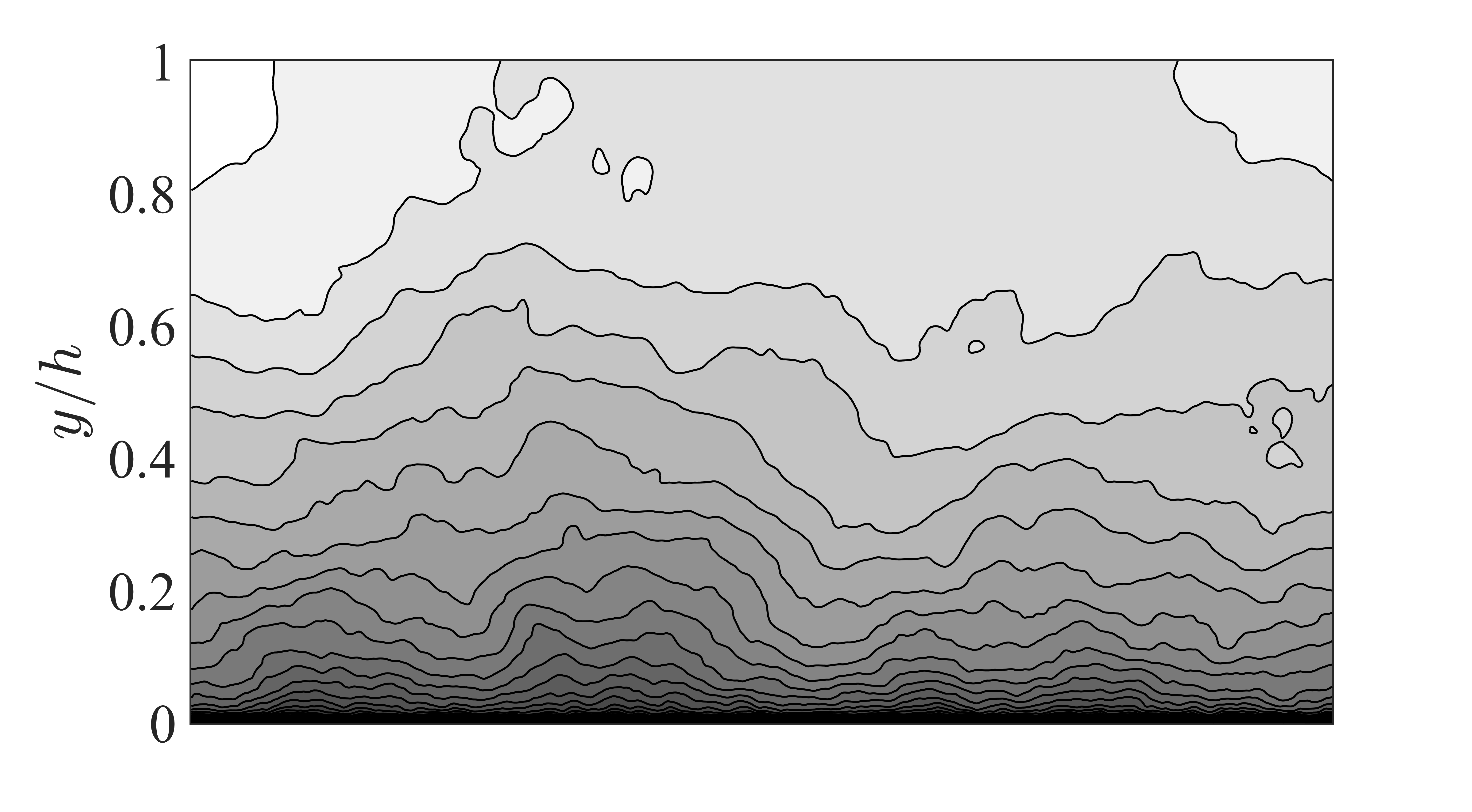
(a)

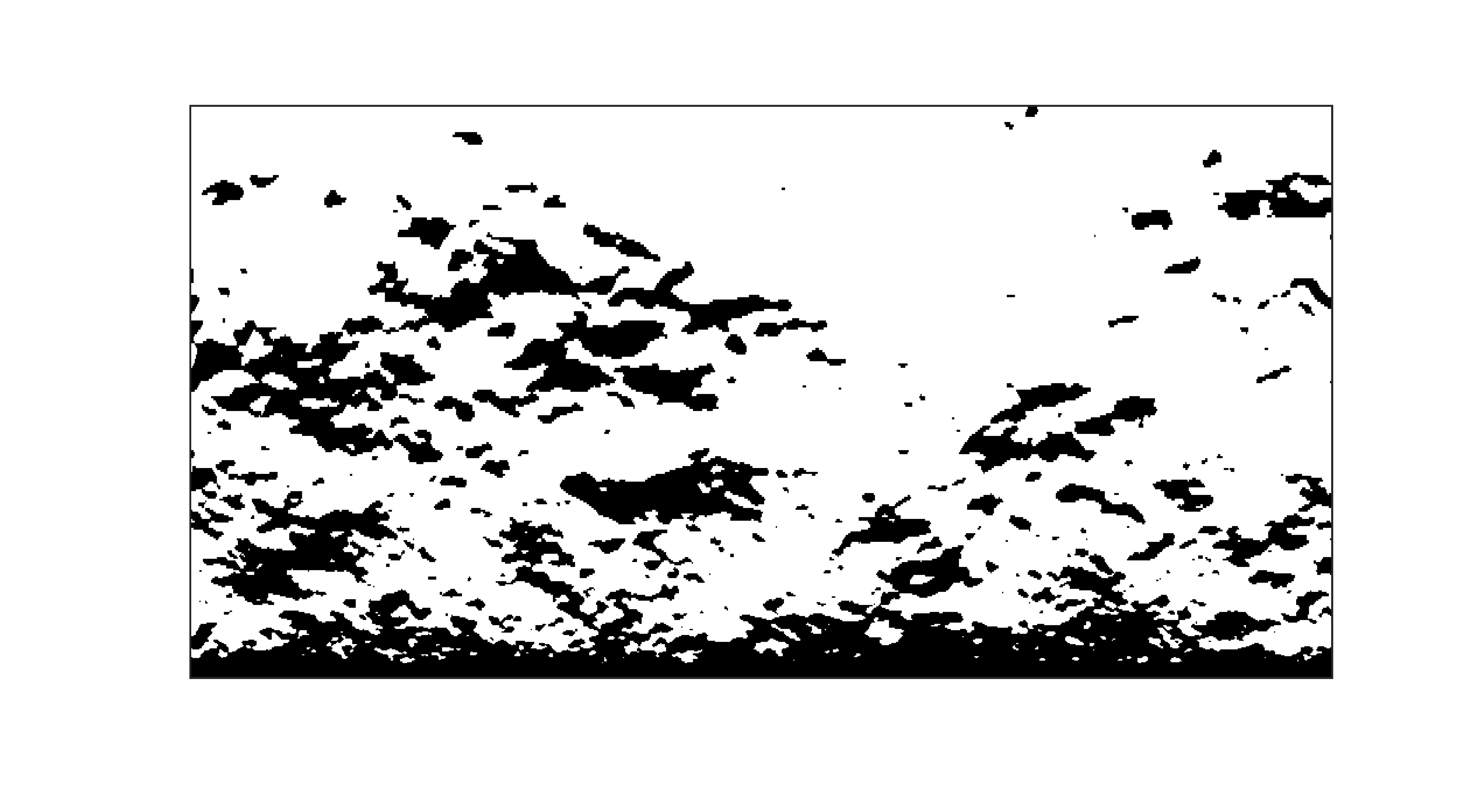
(c)

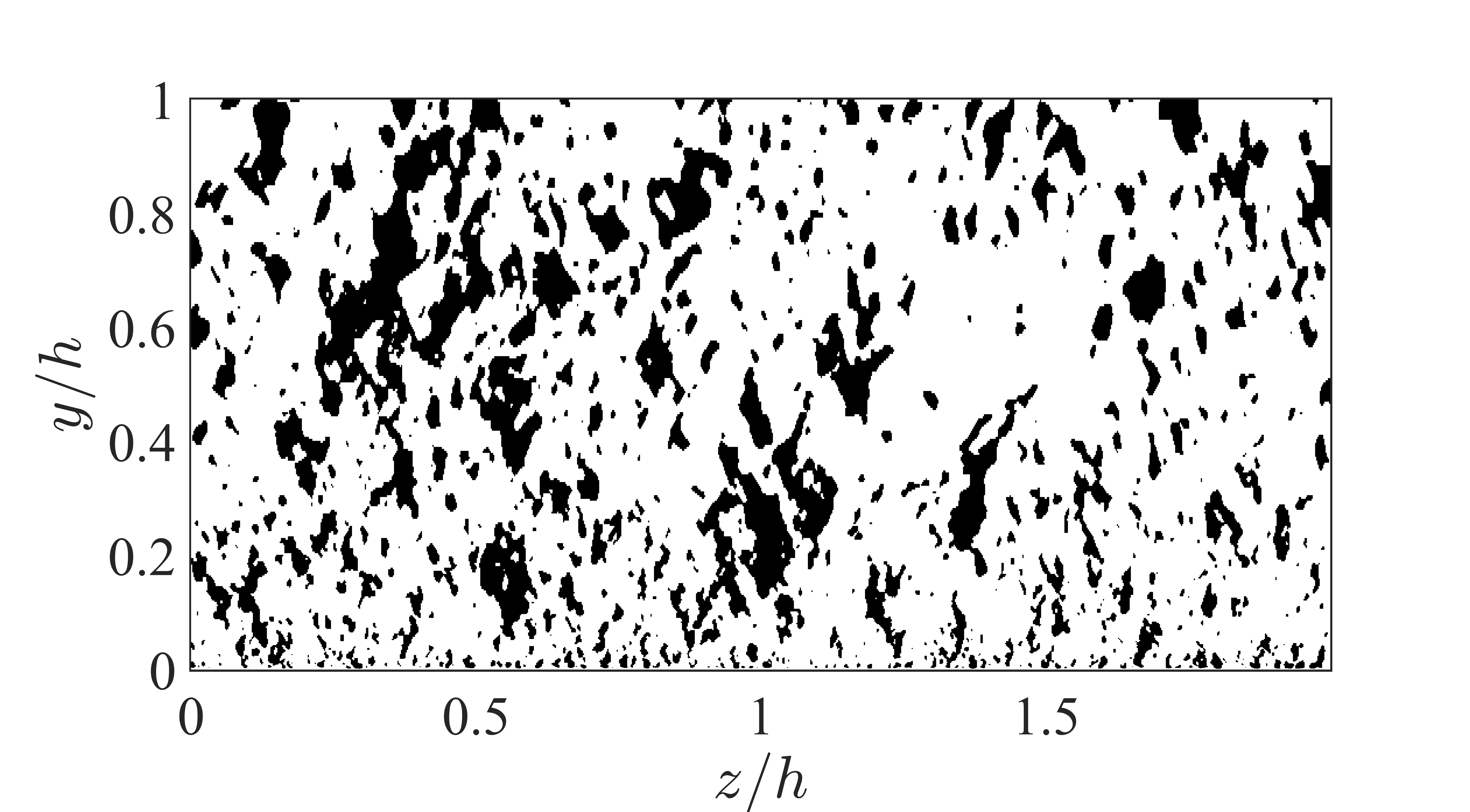
(b)

(d)

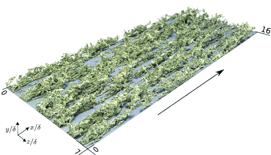
(e)

Figure 3: (a) Cross section of the streamwise velocity, $U$, in a channel at $Re_{\tau}=2000$ [30]. Contours are $U/u_{\tau}=$(0: 0.78: 25), increasing upwards. (b) Vertical derivative of the flow in (a). Dark areas are $\partial_{y}U>3S$ where $S=\langle\partial_{y}U\rangle_{xz}$ is the plane-averaged mean shear. (c) Spanwise derivative. $\partial_{z}U>1.5S$. (d) Magnitude of the cross-plane gradient. $[(\partial_{z}U)^{2}+(\partial_{y}U)^{2}]^{1/2}>3S$. (e) Outer-flow high-velocity streaks, visualised by the perturbation streamwise velocity, $u=2u_{\tau}$. Boundary layer at $Re_{\tau}\approx 1200$–1400. Structures shorter than half the boundary layer thickness, $\delta$, have been removed (reproduced with permission from [58]; credits J.A. Sillero)

This is not necessarily cheap, even if processing a single flow field is usually equivalent to a single time step of the simulation. We have already alluded at the end of the previous section to the difficulty of storing large data sets. Using them is also computationally expensive, because many snapshots have to be analysed, typically iteratively. A rough estimate from the experience of our group is that postprocessing the data set resulting from a simulation requires from two to three times more computer time than the original run. But postprocessing can (and should) be done at leisure over several years, and in collaboration with teams beyond the original simulators, and it provides opportunities that would be unavailable in any other way.

A simple but striking example of how simulation data can help correct misinterpretations due to instrumental limitations is figure 3(a-d), which shows a cross-stream section of the streamwise velocity in a channel, and three versions of the ‘vorticity clefts’ detected by different implementations of the cross-plane gradient. The one-directional gradients in figure 3(b), which simulate the two-dimensional sections in a particular experiment [59, 60], could naively be interpreted as planar fronts separating two-dimensional uniform-momentum layers, and this interpretation has occasionally persisted [61] even if the original group specifically warned otherwise and quantitatively characterised the three dimensional structure [62]. The two-dimensional gradients in figure 3(d) clearly show the tube-like geometry of the uniform-velocity streaks, as is also seen in the three-dimensional representation in figure 3(e). The vertical clefts in figure 3(c) show how easy it is to introduce artefacts from incomplete data.

Another illustrative case is the characterisation of sweeps and ejections in wall-bounded turbulence, which had originally been defined from single-point hot-wire data [63, 64]. The argument was that, because the tangential Reynolds stress can be written as the average of the product of the streamwise and wall-normal velocity fluctuations, $-\langle uv\rangle_{xz}$, where $\langle\rangle_{xz}$ is the average over wall-parallel planes, the regions where both velocities are strong and either $u>0$ and $v<0$ (sweeps) or vice versa (ejections) mark significant locations for momentum transfer. In practice, these two types of regions carry about 60% of the total tangential Reynolds stress in attached wall-bounded turbulent flows [58].

A lot of work has been devoted to such ‘quadrant’ analysis, and a lot has been learned about it from hot wires and particle-image velocimetry [65]. This helped to establish the ‘hairpin packet’ model of wall turbulence [66], although the limited information provided by the experiments, usually at most restricted to two-dimensional sections, resulted in some confusion about the geometrical properties of the objects in question.

It was only when full three-dimensional vorticity and velocity fields became available from direct simulations of turbulent channels and boundary layers that the true geometry of the sweeps and ejections could be clarified [67, 68, 69]. They are three-dimensional structures which separate into wall-attached and wall-detached families, depending of whether their root reaches the wall or not. Most of the momentum transfer is associated with the wall-attached structures, which form a self-similar family of eddies with moderate aspect ratios (length: width: height $\approx$ 3:1:1), organised as spanwise pairs of one sweep and one ejection. These pairs can be interpreted as the two sides of approximately streamwise rollers, which, in turn, are organised as rows along the edges of the streamwise velocity streaks. Sweeps, bringing high-speed fluid towards the wall, are located in the high-velocity streaks, and ejections, moving low-speed fluid away from the wall, are located in the low-speed ones.

These composite objects come in all sizes, from packets of individual vortices near the wall, with spanwise width of the order of 100 wall units and streamwise length of 500–1000 wall units [67], to very large structures of the order of the boundary layer thickness, formed by vortex tangles instead of by single vortices [68, 70, 69].

Given the importance of wall-attached structures, it is a fair question whether they form at the wall and rise, appear away from the wall and sink, or any combination of the two. The resolution of this question either requires the conceptual simulations discussed above, or tracking the structures along their full lifetime. The latter is difficult in the laboratory, because structures travel long distances from the moment they first appear to the point when they can be recognised as strong events, and also because they drift in and out of the two-dimensional sections typically provided by experiments. The answer came from simulation data sets in which the flow variables are stored closely enough in time for individual structures to be followed [42]. It turns out that sweeps are formed away from the wall and move down, and that ejections are formed near the wall and move up. The objects formed by the sweep-ejection pairs do not migrate significantly up or down.

The lack of vertical drift of the pairs suggests that their cause is not the wall but the shear, which, in any case, is the ultimate source of kinetic energy for the turbulent fluctuations [32]. This was confirmed in [71], who repeated the three-dimensional structural analysis for a uniform shear flow with no walls. The results were similar to those in channels, although with some interesting differences. Sweeps and ejections are found in both flows, with similar aspect ratios, and they are located in both cases at the interface between a high- and a low-velocity streak. But the inclination of the associated rollers is different in the two flows. The average inclination in a uniform shear is 45^o, as required by symmetry considerations, but it becomes shallower for detached structures in channels, and almost parallel to the wall for attached pairs. At the same time, the ejection, which is typically located below the sweep, because it comes from the lower-speed fluid below, is of the same size as the sweep in the uniform shear, but shrinks as the pair gets closer to the wall. The same is true for the low-speed streak. The overall conclusion is that the effect of the wall is to hinder the formation of the inclined rollers and of the streaks, rather than to promote them.

Consistent with their location in high- and low-velocity streaks, sweeps advect faster than ejections, and the initially spanwise pair slowly separates in the streamwise direction at the same time as it does vertically. The velocity difference in the two directions is of the order of the friction velocity, $u_{\tau}$, so that the lifetime of the roller can at most be of the order of its turnover time $O(y/u_{\tau})$, where $y$ is both the distance from the wall and the height of the attached eddies. This was confirmed by direct tracking in [42].

It should be clear from the previous discussion that the importance of archived data sets is mainly that they can be used to test theories. Consider a final example. It was known that the main contributor to the evolution equations in shear flows is advection by the mean profile [72], and we have already mentioned that the source of kinetic energy for the fluctuations is their interaction with the mean shear. In that sense, the energy-producing scales of shear turbulence are linear, although nonlinearity dominates further down the cascade. It was established in [73, 74] that the criterion separating the two regimes is the ratio between the eddy turnover time and the deformation time defined by the inverse of the mean shear. When this Corrsin number is large, the shear of the mean velocity profile dominates, and the flow can be considered linearisable. Using only spectral information, the Corrsin number can be defined for the mean flow, or individually for eddies of a given size. The results is that wall-bounded flows are linearisable in the logarithmic and buffer layers, and that the linearisation can only be applied to eddies which are at least as large as their distance from the wall [58]. Geometrically, this suggests that the attached structures, defined above as reaching the wall, are identical to the ‘active’ eddies hypothesised in [75], and that both are just eddies larger than the spectral Corrsin scale. This was tested in [71] using the uniform shear flow. When discussing this flow, we mentioned that the sweeps and ejections in the uniform shear were essentially the same as the attached structures in channels, but this begs the question of which eddies are to be considered attached in a flow without walls. What [71] showed is that the uniform-shear eddies equivalent to the attached ones in channels are those larger than the Corrsin limit. Smaller ones behave like the detached channel structures.

Many similar examples can be mentioned of the use of computers in supporting or falsifying theories or models, from mostly linear ones [76, 77, 78] to the fully nonlinear identification of invariant solutions [79]. Discussing them any further would take us beyond the scope of the present paper, but a recent survey of the properties of structures in wall turbulence and related flows is [58].

4 Trivial simulations and Monte Carlo research

In the previous section we have given examples of how using computers as ‘universal answering’ machines, performing routine searches and conceptual experiments in no more than a few hours, can advance the study of turbulence. The procedure follows the classical scientific method of designing experiments to address a particular question, with the only difference that they are performed computationally. However, because the time spent in each simulation is short, but not trivial, testing more than a few possibilities still requires a ‘heroic’ multi-month effort. A consequence is that experiments tend to be designed carefully, because wild guesses waste valuable simulation time, and that they tend to address incremental questions, rather than revolutionary ones.

A different approach becomes possible once conceptual experiments are cheap enough to be executed at essentially no cost. It is then possible to perform ‘silly’ experiments, just in case they produce something, and to decide a posteriori which results are interesting. In essence, this is equivalent to using a Monte Carlo method to compute the volume of a hypersphere by randomly throwing points and counting which fraction falls within the sphere [80], instead of by careful integration.

Once this level of computational performance has been reached, simulations can be considered tools for creating (or suggesting) questions, rather than just for generating answers. For example, consider a machine that can add ordered pairs of integers by consecutively accumulating units (e.g. $2=1,1\Rightarrow 2+3=1,1,1,1,1$), but which does not know the properties of addition. We can use it to test commutativity by asking whether pairs such as $1+4$ and $4+1$ always give the same result, but this can only be done if we suspect that commutativity exists.

A different approach would be to test a large number of random pairs looking for repetitions, and to ‘notice’ that several pairs give the same result: e.g., $1+9$, $2+8$, etc. Once equivalent pairs are collected into classes (‘10’ in the previous example), somebody, either the machine or the programmer, may look for possible regularities within each class, and wonder, for example, why equivalent pairs tend to come in couples, $2+8=8+2$. It is obvious that such an observation does not constitute a proof of commutativity, but it may be considered as a suggestion that such a property exist, and an invitation to research it more carefully. Although the example is trivial, it illustrates the potential of randomised experiments to be statistically exhaustive, in the sense that they can investigate properties with few preconceived ideas.

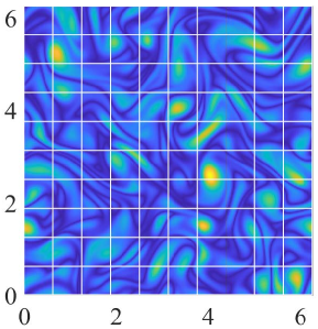
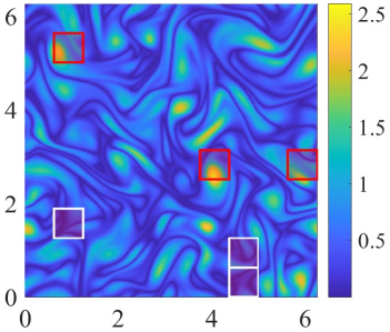
(a)   (b)

Figure 4: (a) Vorticity magnitude in an initial condition to be tested. The overlaid grid is used to select the test subsets. (b) Cells outlined in white are the three least significant ones after $\omega^{\prime}T=7$, where $\omega^{\prime}$ is the root-mean-square vorticity of the initial field. Those outlined in red are the three most significant ones. In this experiment, the vorticity in the subset being modified is substituted by a constant whose magnitude conserves the overall enstrophy, with opposite sign to its original mean.

ProperLabelling$(g,T,A,\mathcal{N})$ Given an initial flow field, $g(\mbox{\boldmath$x$},t=0)$, a target time, $t=T$, and a partition, $A$, of $g$ into subsets. For all subsets $a\in A$ Create a test field by $\overline{g}(a,t=0)\Leftarrow\mathcal{N}(g)$. Evolve $g$ and $\overline{g}$ to $t=T$, using the equations of motion. Compute the perturbation growth, $\varepsilon=\|\overline{g}(T)-g(T)\|$ Iterate over $A$. Output: Label as most (least) significant the $a$’s maximising (minimising) $\varepsilon$. Store $a,\varepsilon$ and all properties of the most (least) significant $a$’s.

Figure 5: Labelling algorithm for selecting the most significant subsets of a flow $g$ under the transformation $\mathcal{N}$.

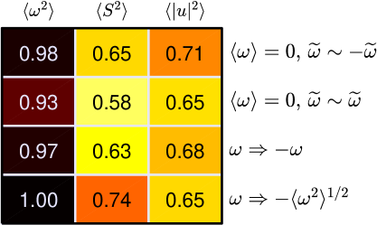
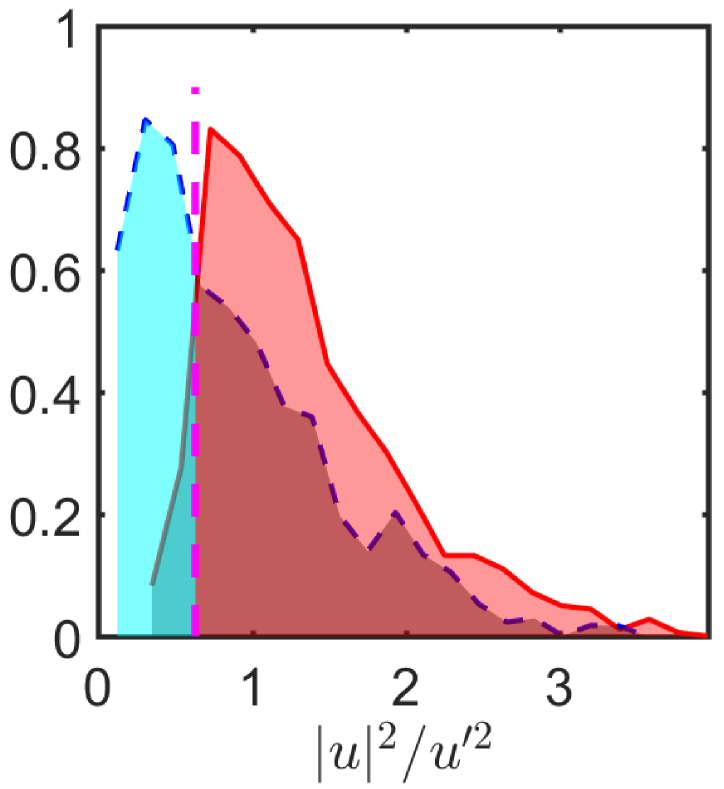
(a)    (b) (c)

Figure 6: (a) Discrimination table for a set of experiments on the flow in figure 5. The labels in the top row are the variables used for discrimination. Those on the right column are the operations used to modify each cell, where $\langle\rangle$ is the average over the cell, and the tilde denotes fluctuations with respect to that average. Values in the table are the discrimination efficiency illustrated in (b,c). (b) Probability density function of the cell enstrophy for:   , most significant cells;            , least significant ones. The vertical line is the optimum discrimination threshold. Conditions are as in figure 5, for the bottom line of the table in (a). (c) As in (b), for the cell kinetic energy.

Consider how such a program could be extended to turbulence, using the example of the identification of coherent structures, which we have already discussed in §3, in relation with sweeps and ejections. The question is how to decide whether there are regions in the flow which are more ‘significant’ than others and, if they are found to exist, to determine their properties. Coherent structures are not natural constructs in fluid mechanics, because the flow is a continuous field with few obvious boundaries along which it can be segmented. Structures have to be defined with some purpose in mind, and tested carefully, because the human mind is prone to impose order even where there is none. A cautionary example are the zodiac constellations, which have been recognised by most cultures in one form or another, and imbued with predictive powers that they are unlikely to have. The fact that most random binary predictions succeed 50% of the time has facilitated the survival of these spurious constructs, even in the absence of supporting evidence, and it should give us pause that this performance is not much worse than the observation, mentioned above, that the sweeps and ejections of wall-bounded flows account for 60% of the total tangential Reynolds stress.

Human researchers, who know the history of a subject, tend to look for incremental improvements on that history, but machines are not biased in the same way. The ability of intelligent machines to ‘reason’ outside human prejudice, even when their intelligence is limited, is probably the most interesting attribute of automatic experimental design.

A simple flow in which to test the automatic identification of structures is decaying isotropic two-dimensional turbulence, where simulations are cheap enough to be run in seconds. There is a wide consensus that this flow is controlled by the interaction of compact vortices [81], and that vortices should probably be found to be the significant flow structures by any reasonable experiment. This ‘ground truth’, together with its relative accessibility to computation, makes two-dimensional turbulence a good example in which to investigate some of the questions posed above. The following discussion follows closely the analysis in [82].

Define significance as the ability of a modification of the initial conditions to change the future behaviour of the flow. In particular, assume that we partition an initial flow field, $g$, into a set of cells $a\in A$, and that we wish to test the effect of modifying in some way the flow within one cell, $g(a,t=0)\Leftarrow\overline{g}=\mathcal{N}(g)$ (see figure 5a). The testing algorithm is sketched in figure 5, and consists of running the reference and modified flows, $g$ and $\overline{g}$, to some target time $T$, and measuring the growth of their separation, $\varepsilon=\|\overline{g}(T)-g(T)\|$. Changes that result in a larger divergence for a given modification procedure are considered to have been applied to more significant regions of the flow. The result is the identification of the (typically three to five) most and least significant cells for each initial flow field and modification procedure (see figure 5b). The final goal is to characterise which properties of a cell can be used to discriminate whether it is significant or not, without running the experiment again.

To that end, we collect as many properties as possible of the most (and least) significant cells, such as the cell enstrophy, kinetic energy, etc., and repeat the process for as many initial conditions (typically 100–200), partitions $(A)$, and experimental transformations $(\mathcal{N})$, as desired. The result is a set of observations, classified into disjoint significance classes, with which to train a human or machine ‘researcher’ to predict significance in terms of cell properties, and to determine which cell properties are most effective as discriminants in each case.

The example in figure 6(a) shows the discrimination table for a set of experiments performed on the flow in figure 5. The columns of the table are possible discriminating variables, which in this case are the mean enstrophy, $\langle\omega^{2}\rangle$, the mean rate of strain, $\langle S^{2}\rangle=\langle 2S_{ij}S_{ij}\rangle$, and the kinetic energy, $\langle|\mbox{\boldmath$u$}|^{2}\rangle=\langle u_{i}u_{i}\rangle$, where $\langle\rangle$ denotes averaging over the cell, and repeated indices imply summation over $i=x,y$. The rows of the table are different modification strategies $(\mathcal{N})$ for the initial conditions, all of which manipulate vorticity. For example, in the bottom line, the vorticity in the cell is substituted by a constant, with opposite sign to the original, and conserving the total enstrophy. The values in the table are the discrimination efficiency illustrated in figure 6(b,c). For each discriminating variable, we construct the probability density function of the most and least significant cells, and determine the threshold that best separates the two histograms. The discrimination index is the fraction of cells that can be correctly classified in this way. In well separated cases, such as the enstrophy in figure 6(b), there are few misclassifications, and the efficiency is close to unity. For variables for which the discrimination is poor, such as the kinetic energy in figure 6(c), approximately half of the cells are misclassified, and the efficiency approaches the random value 0.5.

The table in figure 6(a) shows that the best discriminating variable is always the enstrophy, and that modifying cells with strong vorticity has a stronger effect than modifying weaker ones, confirming our initial guess that intense vortices are the dominant structures in this flow.

 (a)        (b)

Figure 7: (a) Kinetic energy of an initial flow field to be tested, corresponding to the second line from the bottom in (b). Outlined in white are the three least significant cells, and in red are the three most significant ones. In this experiment the velocity in the cell is substituted by a constant with opposite sign to its original mean, with a magnitude that conserves the overall energy. Which velocity component is changed is chosen to maximise the effect. (b) Discrimination efficiency for a set of experiments that change the velocity of individual cells of the flow in (a), as in figure 6(a).

However, figure 7 suggests a more nuanced conclusion. Figure 7(a) is a flow field from the same set of initial conditions as figure 5, but the variable represented is the kinetic energy, which is also intermittent in two-dimensional turbulence [83]. The experiments in figure 7(b) manipulate the velocity. This is more complicated than manipulating the vorticity, because the modified velocity has to satisfy continuity (see [82] for details), and because velocity is a vector, and part of the experimental search is to decide which component to modify. The table in figure 7(b) shows that the best discriminating variable in these cases is the kinetic energy, not the enstrophy, suggesting that there are at least two kinds of coherent structures in two-dimensional turbulence, vortices and high-speed regions, and that they can be identified by different experimental procedures.

Continuing with the interpretation of the above results is beyond the scope of the present paper, whose subject is how computers can contribute to the study of turbulence, not the dynamics of two-dimensional turbulence. But it is interesting that, even in this simple case, random experiments unearth a set of structures that were a priori unexpected. Such results can be considered examples of what we denoted above as machine-generated questions. For example, it is known that high velocities are associated with vortex cores in two-dimensional turbulence [83], suggesting that the two types of features may not be that different, but this does not explain why the optimum discriminating variable is different in the two cases. It is also interesting to highlight the bottom row in figure 7(b), for which the best discriminating variables are the enstrophy and the rate of strain, rather than the energy, even if it represents a velocity manipulation which only differs from the next row by a sign.

In practice, the number of discriminating variables and experimental procedures may be quite higher than in the previous example, and simple threshold discriminators may not be sufficient for a successful classification. There are machine learning algorithms to handle these cases, typically under the name of ensemble learning [84]. Even in the previous example, the joint use of enstrophy and energy as discriminating variables, which can still be done by hand, results in a somewhat better discrimination than the single variables used above. There are also automatic schemes for detecting outliers [85], such as the last line in figure 7(b). Their purpose is often to eliminate them as noise, but, in the present context, it may rather be to highlight interesting cases.

An important aspect of the experiments just described is cost, because trivial turbulence simulations have only recently become possible. Our example uses a $256^{2}$ grid, and each simulation spanning $\omega^{\prime}T=6$ takes about 9 s in a single Xeon core (X5650). Testing each $10\times 10$ partition requires 100 simulations, and each experiment is run 100 times. Each full experiment thus cost 37 core-hours. How many target times and experimental manipulations are tested is up to the researcher. In the present case, it adds another factor of 100, bringing the total to a few thousand core-hours. However, simulations are independent of each other and can be run in parallel, and even a small departmental cluster brings the actual ‘clock’ time to about a week.

To translate these times to three-dimensional isotropic turbulence, consider a $256^{3}$ box. Simulating $u^{\prime}T/L=2$ on a modern GPU (Titan V) takes about two minutes, so that testing a partition of $5^{3}$ cells requires approximately four GPU-hours. Assuming again 100 independent initial conditions brings the cost of a basic experimental test to 15 GPU-days. Again, a small GPU cluster brings it down to a few days, and allows $O(10)$ randomised experiments in a month. While more expensive than the two-dimensional case, this is still affordable.

5 Discussion: competitors or colleagues?

As mentioned in the introduction, the goal of this paper is to promote discussion, and it therefore offers no conclusions. However, we can summarise what we have discussed up to now, and highlight some of the questions that, from the point of view of the author, need to be addressed by the community. The paper has been organised in three sections ordered by the increasing capabilities of computers. The first two sections, which deal with computers as expensive experimental apparatus, or as providers of routine answers to questions posed by the researcher, present few conceptual problems. They represent different ways of doing science as usual. As with all new instruments, computers have led to new discoveries that would have been impossible had they not been available, and we have highlighted some of them. In particular, the availability of four-dimensional data sets, which can be explored in any desired order, and the possibility of performing almost arbitrary conceptual experiments, have advanced our understanding of turbulence well beyond what was available in the 1970’s. The methodology discussed in these two sections can be considered as established.

Section 4 presents a different problem. In essence, the methods discussed there have not yet achieved anything, but they promise to free turbulence research from possible prejudices of the past, and to lead it to fresh territories. In the absence of an ideal ‘very smart graduate student from Mars’, who knows mathematics but does not know enough terrestrial fluid mechanics to be misled by any errors that may have crept into our theoretical models, the suggestion is that we may be able to outsource at least part of our exploratory work to machines which, although not particularly smart, can deal with the Navier–Stokes equations in trivially short times.

In the nomenclature popularised by Kuhn [86], machines do not share the paradigms of trained scientists, and are freer to explore new avenues. While it would be unreasonable to expect what we have called Monte Carlo experimentation to change the paradigms of our discipline, one of the routine roles of research is to collect facts related to the established point of view. The ostensible goal is to reinforce it, but history shows that, occasionally, the resulting observations contradict the established theory, and that the accumulation of such ‘mistakes’ may result in an eventual paradigm shift, or at least in paradigm drift. The hope is that the Monte Carlo research made possible by plentiful computer power can be used as a tool to expedite this process, without prejudging the result, in much the same way as we use machine tools to expedite manufacturing. In essence, if we consider paradigms as optima of understanding, computers can be used to provide the ‘noise’ required to prevent us from getting stuck in a local optimum.

However, we cannot avoid worrying about whether the introduction of this new tool may be different from the previous mechanical ones, and whether it may happen that we do not like the results of machine research. In essence, we have to decide whether we want to cooperate with the machines in this area, or to compete with them.

For example, what about the value of the Kármán constant? We mentioned in §4 that we can compute it quite precisely by blind simulation. Should we allow the machine to conclude that knowing the value of $\kappa$ is the final answer? Should we agree that a better turbulence theory is one that produces a more precise value for that constant? If not, why not? One of the central tenets of science is that the results should be independent of the feelings of the scientist, and it is doubtful from a ‘moral’ perspective whether we should reject useful science, such as a new antibiotic or a better value for a modelling constant, just because we don’t like the way in which it was obtained.

But we also know, or at least this author does, that mathematics are beautiful, and that we may be reluctant to accept, or to be interested in, ugly science. We may need to imbue machines with a sense of aesthetics to make sure that we want to talk to them, or we risk splitting science into useful and beautiful; not necessarily contradictory, but neither necessarily coincident. The problem is more acute if we accept the argument in §4 that the results of randomised experiments are tantamount to questions rather than to answers. Would we be as interested in machine questions as we are in machine answers? Would machine curiosity coincide with human one? Would we even recognise it as such?

Of course, most of these worries are overblown, at least in the short term, because machines are still very far from matching even the most hapless laboratory assistant, but it may not be too early to start discussing how to respond to them when they improve, as they will. Humanity has been through this process before. Javelin throw used to be a useful military skill in which champions were expected to throw as far as possible. It has since been relegated to a sporting event, widely admired but full of restrictive rules intended to prevent ‘ugly’ long throws. Long-range attacks have been outsourced to machines.

We cited at the beginning of §3 a well-known paper whose title asks whether we would be able to understand what is it like to be a bat [48]. The answer in that paper is not very hopeful. The question facing us in the medium term is whether we would be able to recognise a machine as a ‘colleague’.

This work was supported by the European Research Council under the Coturb grant ERC-2014.AdG-669505.

References

- [1] A. E. Brenner, The computing revolution and the physics community, Phys. Today 49 (10) (1996) 24–32.
- [2] M. L. Norman, Probing cosmic mysteries by supercomputer, Phys. Today 49 (10) (1996) 42–48.
- [3] P. Moin, K. Mahesh, Direct numerical simulation: A tool in turbulence research, Ann. Rev. Fluid Mech. 30 (1998) 539–578.
- [4] T. Wu, M. Tegmark, Toward an AI physicist for unsupervised learning (2018). arXiv:1810.10525.
- [5] E. MacCurdy, The notebooks of Leonardo da Vinci, Reynald & Hitchcock, New York, 1939.
- [6] C. Zammattio, A. Marioni, A. M. Brizio, Leonardo, the scientist, McGraw–Hill, New York, 1980.
- [7] G. H. L. Hagen, Über den Bewegung des Wassers in engen cylindrischen Röhren, Poggendorfs Ann. Physik Chemie 46 (1839) 423–442.
- [8] J. M. L. Poiseuille, Recherches expérimentales sur le mouvement des liquides dans les tubes de très petits diamètres, Mém. Savants Etrang. Acad. Sci. Paris 9 (1846) 435–544.
- [9] G. H. L. Hagen, Über den Einfluss der Temperatur auf die Bewegung des Wassers in Röhren, Math. Abh. Akad. Wiss. Berlin (1854) 17–98.
- [10] H. Darcy, Recherches expérimentales rélatives au mouvement de l’eau dans les tuyeaux, Mém. Savants Etrang. Acad. Sci. Paris 17 (1854) 1–268.
- [11] J. Boussinesq, Essai sur la theorie des eaux courantes, Mem. Acad. Sci. Paris 23 (1877) 1–680.
- [12] O. Reynolds, An experimental investigation of the circumstances which determine whether the motion of water shall be direct or sinuous, and of the law of resistance in parallel channels, Phil. Trans. Royal Soc. London 174 (1883) 935–982, papers, ii, 51.
- [13] O. Reynolds, On the dynamical theory of incompressible viscous fluids and the determination of the criterion, Proc. R. Soc. London 56 (1894) 40–45.
- [14] Rouse, H. and Ince, S., History of hydraulics, Dover, New York, 1957.
- [15] H. Lamb, Hydrodynamics, 2nd Edition, Cambridge U. Press, 1895.
- [16] A. N. Kolmogorov, The local structure of turbulence in incompressible viscous fluid for very large Reynolds numbers, Dokl. Akad. Nauk SSSR 30 (1941) 209–303.
- [17] L. Rosenhead, The formation of vortices from a surface of discontinuity, Proc. Roy. Soc. A 134 (1931) 170–192.
- [18] M. M. Koochesfahani, P. E. Dimotakis, Mixing and chemical reactions in a turbulent liquid mixing layer, J. Fluid Mech. 170 (1986) 83–112.
- [19] L. F. Richardson, Weather prediction by numerical process, Cambridge U. Press, 1922.
- [20] J. C. R. Hunt, Lewis Fry Richardson and his contributions to mathematics, meteorology, and models of conflict, Ann. Rev. Fluid Mech. 30 (1998) xiii–xxxvi.
- [21] P. Lynch, Richardson’s forecast-factory: the $64,000 question, Met. Mag. 122 (1993) 69–70.
- [22] R. W. Seidel, From Mars to Minerva: The origins of scientific computing in the AEC labs, Phys. Today 49 (10) (1996) 33–39.
- [23] N. Macrae, John von Neumann – the scientific genius who pioneered the modern computer, Am. Math. Soc., 1999.
- [24] J. G. Charney, R. Fjörtoft, J. von Neumann, Numerical integration of the barotropic vorticity equation, Tellus 2 (1950) 237–254.
- [25] G. Bell, D. H. Bailey, J. Dongarra, A. H. Karp, K. Walsh, A look back on 30 years of the Gordon Bell prize, Int. J. High Speed C. 31 (2017) 469–484.
- [26] S. A. Orszag, G. S. Patterson, Numerical simulation of three-dimensional homogeneous isotropic turbulence, Phys. Rev. Lett. 16 (1972) 76–79.
- [27] J. Jiménez, A. A. Wray, P. G. Saffman, R. S. Rogallo, The structure of intense vorticity in isotropic turbulence, J. Fluid Mech. 255 (1993) 65–90.
- [28] Y. Kaneda, T. Ishihara, High-resolution direct numerical simulation of turbulence, J. Turbul. 7 (2006) N20.
- [29] J. Kim, P. Moin, R. D. Moser, Turbulence statistics in fully developed channel flow at low Reynolds number, J. Fluid Mech. 177 (1987) 133–166.
- [30] S. Hoyas, J. Jiménez, Scaling of the velocity fluctuations in turbulent channels up to , Phys. Fluids 18 (2006) 011702.
- [31] M. Lee, R. D. Moser, Direct numerical simulation of turbulent channel flow up to , J. Fluid Mech. 774 (2015) 395–415.
- [32] H. Tennekes, J. L. Lumley, A first course in turbulence, MIT Press, 1972.
- [33] J. Jiménez, Computing high-Reynolds number flows: Will simulations ever substitute experiments?, J. Turbul. 4 (2003) N22.
- [34] S. Zimmerman, J. Philip, J. Monty, A. Talamelli, I. Marusic, B. Ganapathisubramani, R. J. Hearst, G. Bellani, R. Baidya, M. Samie, et al., A comparative study of the velocity and vorticity structure in pipes and boundary layers at friction reynolds numbers up to , J. Fluid Mech. 869 (2019) 182–213.
- [35] J. Jiménez, Cascades in wall-bounded turbulence, Ann. Rev. Fluid Mech. 44 (2012) 27–45.
- [36] S. Hoyas, M. Oberlack, S. Kraheberger, F. Alcántara-Avila, Turbulent channel flow at , in: Proc. Div. Fluid Dyn., Am. Phys. Soc., 2018, pp. G–38.
- [37] A. Gungor, Y. Maciel, M. Simens, J. Soria, Scaling and statistics of large-defect adverse pressure gradient turbulent boundary layers, Int. J. Heat Fluid Flow 59 (2016) 109–124.
- [38] R. Vinuesa, P. S. Negi, M. Atzori, A. Hanifi, D. S. Henningson, P. Schlatter, Turbulent boundary layers around wing sections up to , Int. J. Heat Fluid Flow 72 (2018) 86–99.
- [39] H. Teng, N. Liu, X. Lu, B. Khomami, Turbulent drag reduction in plane Couette flow with polymer additives: a direct numerical simulation study, J. Fluid Mech. 846 (2018) 482–507. doi:10.1017/jfm.2018.242.
- [40] E. Perlman, R. Burns, Y. Li, C. Meneveau, Data exploration of turbulence simulations using a database cluster, in: Proc. SC07, ACM, New York, 2007, pp. 23.1–23.11.
- [41] J. A. Sillero, J. Jiménez, Editorial opinion: public dissemination of raw turbulence data, J. Physics: Conf. Ser. 708 (2016) 011002.
- [42] A. Lozano-Durán, J. Jiménez, Time-resolved evolution of coherent structures in turbulent channels: characterization of eddies and cascades, J. Fluid Mech. 759 (2014) 432–471.
- [43] A. Vela-Martín, M. P. Encinar, A. García-Gutiérrez, J. Jiménez, A second-order consistent, low-storage method for time-resolved channel flow simulations, (2018). arXiv:1808.06461.
- [44] J. N. Butler, D. R. Quarrie, Data acquisition and analysis in extremely high data rate experiments, Phys. Today 49 (10) (1996) 50–56.
- [45] M. Hultmark, M. Vallikivi, S. C. C. Bailey, A. J. Smits, Turbulent pipe flow at extreme Reynolds numbers, Phys. Rev. Lett. 108 (2012) 094501.
- [46] K. R. Sreenivasan, On the universality of the Kolmogorov constant, Phys. Fluids 7 (1995) 2778–2784.
- [47] Y. Kaneda, T. Ishihara, M. Yokokawa, K. Itakura, A. Uno, Energy dissipation rate and energy spectrum in high resolution direct numerical simulations of turbulence in a periodic box, Phys. Fluids 15 (2003) L21–L24.
- [48] T. Nagel, What is it like to be a bat?, Philos. Rev. 83 (1974) 435–450.
- [49] R. S. Rogallo, P. Moin, Numerical simulations of turbulent flows, Ann. Rev. Fluid Mech. 16 (1984) 99–137.
- [50] M. Germano, U. Piomelli, P. Moin, W. Cabot, A dynamic subgrid-scale eddy viscosity model, Phys. Fluids A 3 (1991) 1760–1765.
- [51] V. Borue, S. A. Orszag, Forced three-dimensional homogeneous turbulence with hyperviscosity, Europhys. Lett. 29 (1995) 687–692.
- [52] Z. She, E. Jackson, Constrained Euler system for Navier–Stokes turbulence, Phys. Rev. Lett. 70 (1993) 1255–1258.
- [53] J. Kim, On the structure of wall-bounded turbulent flows, Phys. Fluids 26 (1983) 2088–2097.
- [54] J. Jiménez, A. Pinelli, The autonomous cycle of near-wall turbulence, J. Fluid Mech. 389 (1999) 335–359.
- [55] Y. Mizuno, J. Jiménez, Wall turbulence without walls, J. Fluid Mech. 723 (2013) 429–455.
- [56] J. Jiménez, P. Moin, The minimal flow unit in near-wall turbulence, J. Fluid Mech. 225 (1991) 213–240.
- [57] O. Flores, J. Jiménez, Hierarchy of minimal flow units in the logarithmic layer, Phys. Fluids 22 (2010) 071704.
- [58] J. Jiménez, Coherent structures in wall-bounded turbulence, J. Fluid Mech. 842 (2018) P1.
- [59] C. D. Meinhart, R. J. Adrian, On the existence of uniform momentum zones in a turbulent boundary layer, Phys. Fluids 7 (1995) 694–696.
- [60] R. J. Adrian, C. D. Meinhart, C. D. Tomkins, Vortex organization in the outer region of the turbulent boundary layer, J. Fluid Mech. 422 (2000) 1–54.
- [61] J. Klewicki, P. Fife, T. Wei, P. McMurtry, A physical model of the turbulent boundary layer consonant with mean momentum balance structure, Phil. Trans. R. Soc. London, Ser. A 365 (2007) 823–839.
- [62] C. D. Tomkins, R. J. Adrian, Spanwise structure and scale growth in turbulent boundary layers, J. Fluid Mech. 490 (2003) 37–74.
- [63] J. M. Wallace, H. Eckelmann, R. S. Brodkey, The wall region in turbulent shear flow, J. Fluid Mech. 64 (1972) 39–48.
- [64] S. S. Lu, W. W. Willmarth, Measurements of the structure of the Reynolds stress in a turbulent boundary layer, J. Fluid Mech. 60 (1973) 481–511.
- [65] K. T. Christensen, R. J. Adrian, Statistical evidence of hairpin vortex packets in wall turbulence, J. Fluid Mech. 431 (2001) 433–443.
- [66] R. J. Adrian, Hairpin vortex organization in wall turbulence, Phys. Fluids. 19 (2007) 041301.
- [67] S. K. Robinson, Coherent motions in the turbulent boundary layer, Ann. Rev. Fluid Mech. 23 (1991) 601–639.
- [68] J. C. del Álamo, J. Jiménez, P. Zandonade, R. D. Moser, Self-similar vortex clusters in the logarithmic region, J. Fluid Mech. 561 (2006) 329–358.
- [69] A. Lozano-Durán, O. Flores, J. Jiménez, The three-dimensional structure of momentum transfer in turbulent channels, J. Fluid Mech. 694 (2012) 100–130.
- [70] O. Flores, J. Jiménez, J. C. del Álamo, Vorticity organization in the outer layer of turbulent channels with disturbed walls, J. Fluid Mech. 591 (2007) 145–154.
- [71] S. Dong, A. Lozano-Durán, A. Sekimoto, J. Jiménez, Coherent structures in statistically stationary homogeneous shear turbulence, J. Fluid Mech. 816 (2017) 167–208.
- [72] J. Jiménez, How linear is wall-bounded turbulence?, Phys. Fluids 25 (2013) 110814.
- [73] S. Corrsin, Local isotropy in turbulent shear flow, Res. Memo 58B11, NACA (1958).
- [74] S. G. Saddoughi, S. V. Veeravali, Local isotropy in turbulent boundary layers at high Reynolds numbers, J. Fluid Mech. 268 (1994) 333–372.
- [75] A. A. Townsend, The structure of turbulent shear flow, Cambridge U. Press, 1976.
- [76] J. C. del Álamo, J. Jiménez, Linear energy amplification in turbulent channels, J. Fluid Mech. 559 (2006) 205–213.
- [77] B. J. McKeon, A. S. Sharma, A critical-layer framework for turbulent pipe flow, J. Fluid Mech. 658 (2010) 336–382.
- [78] J. Jiménez, Direct detection of linearized bursts in turbulence, Phys. Fluids 27 (2015) 065102.
- [79] G. Kawahara, M. Uhlmann, L. van Veen, The significance of simple invariant solutions in turbulent flows, Ann. Rev. Fluid Mech. 44 (2012) 203–225.
- [80] J. M. Hammersley, D. C. Handscomb, Monte Carlo methods, Chapman and Hall, 1964.
- [81] J. C. McWilliams, The vortices of two-dimensional turbulence, J. Fluid Mech. 219 (1990) 361–385.
- [82] J. Jiménez, Machine-aided turbulence theory, J. Fluid Mech. 854 (2018) R1.
- [83] J. Jiménez, Algebraic probability density functions in isotropic two-dimensional turbulence, J. Fluid Mech. 313 (1996) 223–240.
- [84] L. Rokach, Ensemble-based classifiers, Art. Intell. Rev. 33 (2010) 1–39.
- [85] V. J. Hodge, A survey of outlier detection methodologies, Art. Intell. Rev. 22 (2004) 85–126.
- [86] T. S. Kuhn, The structure of scientific revolutions, 2nd Edition, Chicago U. Press, 1970.