Abstract

We propose $\beta$-graph embedding for robustly learning feature vectors from data vectors and noisy link weights. A newly introduced empirical moment $\beta$-score reduces the influence of contamination and robustly measures the difference between the underlying correct expected weights of links and the specified generative model. The proposed method is computationally tractable; we employ a minibatch-based efficient stochastic algorithm and prove that this algorithm locally minimizes the empirical moment $\beta$-score. We conduct numerical experiments on synthetic and real-world datasets.

1 INTRODUCTION

In the past few decades, graph embedding (GE) that learns feature vectors of given graph nodes had high level of demand in a broad range of fields. Just an example among many, embedding social networks whose nodes and link weights represent users and their relationships, respectively, produces user feature vectors. Traditional multivariate statistical methods, such as clustering and classification, can then be applied to these feature vectors (Yan et al.,, 2007; Goyal and Ferrara,, 2018), whereas these analysis methods, in general, cannot be applied directly to unprocessed graph nodes.

Classical GE typified by spectral GE (SGE; see Chung,, 1997; Belkin and Niyogi,, 2001) computes feature vectors so that their inner product similarities represent the link weights, and the locality-preserving projections (LPP; see He and Niyogi,, 2004) extends SGE so that it additionally considers pre-obtained data vectors of nodes. LPP computes feature vectors by linear transformation of data vectors; the local configuration of vectors is partially preserved through the transformation. Although SGE and LPP experimentally demonstrate reasonable performance, their computational complexity is high owing to eigendecomposition.

To reduce the high computational complexity, Tang et al., (2015) proposed a computationally efficient GE named large-scale information network embedding (LINE), which is based on the stochastic maximization of the likelihood over link weights. Although LINE, as well as SGE, does not consider pre-obtained data vectors of nodes, the graph embedding can be extended to utilize the data vectors by incorporating neural networks (Wang et al.,, 2016; Kipf and Welling,, 2017; Dai et al.,, 2018). The graph embedding can be further extended to deal with multi-view setting (Okuno et al.,, 2018), where each vector is assigned to one of multiple types of vectors (e.g. image vectors, text vectors) with different dimensionalities.

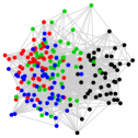
(a) $\beta=0$

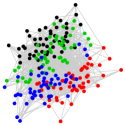
(b) $\beta=0.5$

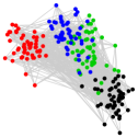
(c) $\beta=1.0$

Figure 1: Proposed $\beta$-GE applied to noisy graph with four clusters. 1(a) corresponds to the existing likelihood-based GE. 1(c) reduces the influence of contamination in noisy link weights. See Section 4.1 for detailed settings.

Although these GEs have been successful in many applications, their performance relies on the quality of observed link weights. However, these observed link weights, in practice, may contain noise. We especially call the link weights with noise as noisy link weights. As shown in Figure 1(a), the noise may degrade the GE’s performance; existing GE is hard to recover the underlying cluster structure from noisy link weights. To overcome this problem, GE should be robustified.

In order to capture the underlying link structure through the noisy link weights, noise-tolerant loss functions can be used. Although a variety of noise-tolerant loss functions have been considered in robust statistics, there have been only a few attempts at using such a noise-tolerant loss function in GE. To the best of the authors’ knowledge, only Pang and Yuan, (2010) and Zhang et al., (2014) have incorporated noise-tolerant $\ell_{1}$- and $\ell_{2,1}$-norm-based loss functions into classical GE. Although these particular types of loss functions are experimentally demonstrated to alleviate the adverse effect of outlier data vectors, they are not theoretically guaranteed to be robust against noisy link weights.

To obtain theoretically-guaranteed robust GE, we attempt to employ $\beta$-score, that robustly measures the difference between two non-negative functions. $\beta$-score is also called as density-power score (Kanamori and Fujisawa,, 2014, 2015), and it is especially called as $\beta$-cross entropy (see, e.g. Futami et al.,, 2018) if the two non-negative functions are limited to probability density function (pdf) or probability mass function (pmf). It is well known that Kullback-Leibler divergence is expressed as the difference of two cross-entropies ($\beta=0$), and quite similarly $\beta$-divergence (Cichocki et al.,, 2010), which is also known as density-power divergence (Basu et al.,, 1998), is expressed as the difference of two $\beta$-cross entropies.

By specifying Poisson distribution for link weights, a probabilistic generative model of GE has been considered (Okuno et al.,, 2018), and $\beta$-score can be applied to this model. However, naively applying $\beta$-score to the probabilistic generative model of GE has two disadvantages: $\beta$-score in this setting is (i) computationally intractable, and (ii) sensitive to distributional misspecification of the generative model, because $\beta$-score measures the difference between two probabilistic models.

In order to avoid these two disadvantages, we introduce moment $\beta$-score that measures the difference in terms of the expected values instead of probability distributions of link weights. The moment $\beta$-score is estimated by empirical moment $\beta$-score (EMBS), which is robust against noise in link weights, and is also carefully designed to be (i) computationally tractable, and (ii) free from the distributional specification. By incorporating EMBS into existing likelihood-based GE using the probabilistic generative model of link weights, we propose a theoretically proven robust GE named $\beta$-graph embedding ($\beta$-GE). This new method naturally extends the likelihood-based GE because the EMBS reduces to the negative log-likelihood of link weights as $\beta\downarrow 0$.

Our contribution is summarized as follows.

1. We propose a novel EMBS, that is a robust score function against noise in link weights as shown in Theorem 3.1. EMBS is also computationally tractable and it is free from the distributional specification.

2. We propose $\beta$-GE by simply incorporating the newly proposed EMBS into existing likelihood-based GE (Section 3.3). As far as we know, $\beta$-GE is the first GE whose robustness is theoretically shown.

3. We propose an efficient minibatch-based stochastic algorithm, which can be proved to locally minimize the EMBS (Section 3.5).

4. We conduct experiments on both synthetic and real-world datasets (Section 4).

2 LIKELIHOOD-BASED GRAPH EMBEDDING

In this section, we review existing likelihood-based GE. Throughout this paper, we consider a setting similar to that presented in Okuno et al., (2018). Although only single-view graph embedding is considered below, its extension to multi-view setting is straightforward as explained in Section 3.7.

Our dataset consists of data vectors $\{\boldsymbol{x}_{i}\}_{i=1}^{n}$ and link weights $\{w_{ij}\}_{(i,j)\in\mathcal{I}_{n}}$, where $\mathcal{I}_{n}:=\{(i,j)\in\mathbb{N}^{2}\mid 1\leq i<j\leq n\}$. The $p$-dimensional data vector $\boldsymbol{x}_{i}\in\mathcal{X}$ takes values in a compact set $\mathcal{X}\subset\mathbb{R}^{p}$. The link weight $w_{ij}\in\{0,1,2,\ldots\}$ is non-negative integer, and it represents the strength of association between $\boldsymbol{x}_{i}$ and $\boldsymbol{x}_{j}$.

Similarly to existing methods (Perozzi et al.,, 2014; Tang et al.,, 2015; Grover and Leskovec,, 2016; Kipf and Welling,, 2016), which employ Bernoulli-based models for considering binary weights, Okuno et al., (2018) employs a Poisson-based model

$$w_{ij}\mid\boldsymbol{x}_{i},\boldsymbol{x}_{j} \overset{\text{indep.}}{\sim}\text{Po}(\mu_{\boldsymbol{\theta}}(\boldsymbol{x}_{i},\boldsymbol{x}_{j}))$$ (1)

by taking $w_{ij}$ as random variables for all $(i,j)\in\mathcal{I}_{n}$. Note that the model (1) does not restrict weights $\{w_{ij}\}$ to be binary. The conditional expected value $E(w_{ij}|\boldsymbol{x}_{i},\boldsymbol{x}_{j})$ is specified by a symmetric, continuous, and non-negative function $\mu_{\boldsymbol{\theta}}(\boldsymbol{x}_{i},\boldsymbol{x}_{j})$, which represents a similarity between two data vectors $\boldsymbol{x}_{i},\boldsymbol{x}_{j}\in\mathcal{X}$, where $\boldsymbol{\theta}\in\boldsymbol{\Theta}$ is a parameter vector and $\boldsymbol{\Theta}\subset\mathbb{R}^{q}$ is a non-empty compact set. Although any symmetric, continuous, and non-negative function can be used as the expected weight function, in this paper, the function is specified as

$$\log\mu_{\boldsymbol{\theta}}(\boldsymbol{x}_{i},\boldsymbol{x}_{j}):=\langle f_{\boldsymbol{\psi}}(\boldsymbol{x}_{i}),f_{\boldsymbol{\psi}}(\boldsymbol{x}_{j})\rangle-\gamma,$$ (2)

where $f_{\boldsymbol{\psi}}:\mathbb{R}^{p}\to\mathbb{R}^{K}$ is arbitrary continuous map whose parameter vector is $\boldsymbol{\psi}$, $\gamma\in\mathbb{R}$ is a scaling parameter regularizing the sparseness of $\{w_{ij}\}$, and $\boldsymbol{\theta}$ denotes $(\boldsymbol{\psi},\gamma)$. Typically, a NN or linear transformation is used as $f_{\boldsymbol{\psi}}$, and the inner product similarity (IPS) between two NNs $\langle f_{\boldsymbol{\psi}}(\boldsymbol{x}_{i}),f_{\boldsymbol{\psi}}(\boldsymbol{x}_{j})\rangle$ is also known as siamese-style similarity (Bromley et al.,, 1994).

IPS is used for a wide variety of GEs (Wang et al.,, 2016; Kipf and Welling,, 2016; Hamilton et al.,, 2017), and has been proven to approximate arbitrary positive-definite (PD) similarities (Okuno et al.,, 2018, Theorem 5.1). In addition, equation (2), which incorporates a new parameter $\gamma\in\mathbb{R}$ into IPS, is specifically called constantly-shifted IPS (C-SIPS), and is proved to approximate conditionally PD similarities, a wider class of similarities than PD similarities (Okuno and Shimodaira,, 2019, Theorem 4.2). Thus, C-SIPS has a sufficiently high representation capability.

Once the optimal $\boldsymbol{\hat{\theta}}=(\boldsymbol{\hat{\psi}},\hat{\gamma})$ is obtained, data vectors $\{\boldsymbol{x}_{i}\}$ can be transformed to feature vectors $\{\boldsymbol{y}_{i}\}$ as

$$\mathbb{R}^{p}\supset\mathcal{X}\ni\boldsymbol{x}_{i}\mapsto\boldsymbol{y}_{i}:=f_{\boldsymbol{\hat{\psi}}}(\boldsymbol{x}_{i})\in\mathbb{R}^{K}$$ (3)

for all $i=1,2,\ldots,n$. The IPS $\langle\boldsymbol{y}_{i},\boldsymbol{y}_{j}\rangle$ of obtained feature vectors $\{\boldsymbol{y}_{i}\}$ indicates the similarity between data vectors $\boldsymbol{x}_{i},\boldsymbol{x}_{j}$. This transformation usually reduces the dimensionality of data vectors from $p$ to $K(\leq p)$. Thus, the obtained vectors are expected to reduce their redundancy while considering the information on link weights. Obtaining the vector representations $\{\boldsymbol{y}_{i}\}$ by considering the link weights $\{w_{ij}\}$ is formally called GE.

One simple way to obtain the optimal parameter $\boldsymbol{\hat{\theta}}$ is to minimize the negative log-likelihood

$$L_{0,n}(\boldsymbol{\theta}) :=-\log\mathbb{P}(\{w_{ij}\}_{(i,j)\in\mathcal{I}_{n}}\mid\{\boldsymbol{x}_{i}\}_{i=1}^{n})$$

(4)

which is based on the Poisson model (1). By minimizing this negative log-likelihood, we obtain the maximum likelihood estimator (MLE)

$$\boldsymbol{\hat{\theta}}_{0}=(\boldsymbol{\hat{\psi}}_{0},\hat{\gamma}_{0}):=\operatorname*{arg\,min}_{\boldsymbol{\theta}\in\boldsymbol{\Theta}}L_{0,n}(\boldsymbol{\theta}),$$

which specifies the optimal NN $f_{\boldsymbol{\hat{\psi}}_{0}}$ and the optimal scaling factor $\hat{\gamma}_{0}\geq 0$. The above-mentioned procedure using MLE to obtain feature vectors is called likelihood-based GE in this paper.

3 $\beta$-GRAPH EMBEDDING

Although the existing likelihood-based GE explained in Section 2 had some success, MLEs in general are susceptible to contamination in data, because log-likelihood can be strongly influenced by noise. In Section 3.1, we review $\beta$-score and related divergence which have been developed in robust statistics for robustifying the log-likelihood. However, naively applying the $\beta$-score to the model (1) has two disadvantages as explained in Section 3.2. To overcome the drawbacks, we introduce moment $\beta$-score that robustly measures the difference between the underlying correct expected weights of links and the specified generative model, and propose its empirical estimation called empirical moment $\beta$-score (EMBS) in Section 3.3. Then, we propose robust $\beta$-GE equipped with EMBS. In Section 3.4, we theoretically prove that EMBS is robust against noise in link weights. In Section 3.5, we introduce a minibatch-based efficient stochastic algorithm, and prove that the algorithm locally minimizes EMBS. In Section 3.6, we discuss the selection of $\beta$. Finally, we extend $\beta$-GE to a multi-view setting in Section 3.7.

3.1 $\beta$-Score for Non-negative Functions

Our idea for robustifying the likelihood-based GE is to employ $\beta$-score, that is originally called as density-power score (Kanamori and Fujisawa,, 2014, 2015). $\beta$-score robustly measures the difference between two non-negative functions as follows.

We consider a random variable $\boldsymbol{z}$ taking a value in some set $\mathcal{Z}$, and consider a set of non-negative functions $\mathcal{P}(\mathcal{Z}):=\{f:\mathcal{Z}\to\mathbb{R}_{\geq 0}\}$. For non-negative functions $g,f,\nu\in\mathcal{P}(\mathcal{Z})$, we define $\beta$-score as

$$\scalebox{0.85}{$\displaystyle u_{\beta}^{\boldsymbol{z}}(g,f;\nu):=$}\begin{cases}\scalebox{0.85}{$\displaystyle-\sum_{\boldsymbol{z}\in\mathcal{Z}}g(\boldsymbol{z})\nu(\boldsymbol{z})\frac{f(\boldsymbol{z})^{\beta}-1}{\beta}+\sum_{\boldsymbol{z}\in\mathcal{Z}}\nu(\boldsymbol{z})\frac{f(\boldsymbol{z})^{1+\beta}}{1+\beta}$}\\ \hskip 100.00015pt(\boldsymbol{z}\text{ is discrete})\\ \scalebox{0.85}{$\displaystyle-\int_{\mathcal{Z}}g(\boldsymbol{z})\nu(\boldsymbol{z})\frac{f(\boldsymbol{z})^{\beta}-1}{\beta}\mathrm{d}\boldsymbol{z}+\int_{\mathcal{Z}}\nu(\boldsymbol{z})\frac{f(\boldsymbol{z})^{1+\beta}}{1+\beta}\mathrm{d}\boldsymbol{z}$}\\ \hskip 90.00014pt(\boldsymbol{z}\text{ is continuous})\\ \end{cases}$$

where $\beta>0$ is a user-specified tuning parameter. For any fixed $g\in\mathcal{P}(\mathcal{Z})$, the minimizer $f\in\mathcal{P}(\mathcal{Z})$ of $u_{\beta}^{\boldsymbol{z}}(g,f;\nu)$ is known to be $f=g$, in the sense that $f(\boldsymbol{z})=g(\boldsymbol{z})$ over the support of $\nu$. If $\nu(\boldsymbol{z})=1$ for all $\boldsymbol{z}\in\mathcal{Z}$, we abbreviate above $\beta$-score by $u_{\beta}^{\boldsymbol{z}}(g,f)$.

Let us consider the special case where the functions $f,g$ are restricted to be pdf or pmf, and they are denoted by $q,p$, respectively. Then, $\beta$-score $u_{\beta}^{\boldsymbol{z}}(q,p)$ is called $\beta$-cross entropy (see, e.g. Futami et al.,, 2018), and $D_{\beta}(q,p):=u_{\beta}^{\boldsymbol{z}}(q,p)-u_{\beta}^{\boldsymbol{z}}(q,q)$ is known as $\beta$-divergence (Cichocki et al.,, 2010) or density-power divergence (Basu et al.,, 1998), which belongs to the Bregman-divergence family (Bregman,, 1967). In particular, $D_{\beta}(q,p)$ reduces to Kullback-Leibler divergence as $\beta\downarrow 0$.

$\beta$-score has also been used for unnormalized models (Kanamori and Fujisawa,, 2015) defined as $cp(\boldsymbol{z})$ where $c\geq 0$ is a scaling parameter and $p(\boldsymbol{z})$ is pdf or pmf. For contaminated $q=c_{0}q_{0}+(1-c_{0})r$ with outlier distribution $r$ and contamination rate $1-c_{0}$, the $\beta$-score $\min_{c\in(0,1]}u_{\beta}^{\boldsymbol{z}}(q,cp)$ is equivalent to the “$\gamma$-divergence” between $q$ and $p$, which robustly measures the difference beween $q_{0}$ and $p$ (Jones et al.,, 2001; Fujisawa and Eguchi,, 2008).

Although $\beta$-score can measure the difference between arbitrary non-negative functions, it has only been applied to probability distributions and unnormalized models as seen above. We call $\beta$-score considering only these cases as probability $\beta$-score. This is different from our usage of $\beta$-score introduced in Section 3.3.

3.2 Two Disadvantages of Naively Applying $\beta$-Score to GE

Probability $\beta$-score can be employed for GE. Considering a conditional pdf $q$ of $w_{ij}\mid\boldsymbol{x}_{i},\boldsymbol{x}_{j}$ and the probabilistic generative model $p_{\boldsymbol{\theta}}$ defined in (1), we may minimize

$$E_{\mathcal{X}^{2}}(u_{\beta}^{(w_{12}\mid\boldsymbol{x}_{1},\boldsymbol{x}_{2})}(q,p_{\boldsymbol{\theta}})),$$ (5)

whose empirical estimation is

$$\frac{1}{|\mathcal{I}_{n}|}\sum_{(i,j)\in\mathcal{I}_{n}}u_{\beta}^{(w\mid\boldsymbol{x}_{i},\boldsymbol{x}_{j})}(\hat{q}_{ij},p_{\boldsymbol{\theta}})$$

$$\hskip 10.00002pt=-\frac{1}{|\mathcal{I}_{n}|}\sum_{(i,j)\in\mathcal{I}_{n}}\frac{p_{\boldsymbol{\theta}}(w_{ij}\mid\boldsymbol{x}_{i},\boldsymbol{x}_{j})^{\beta}-1}{\beta}$$

$$\hskip 30.00005pt+\frac{1}{|\mathcal{I}_{n}|}\sum_{(i,j)\in\mathcal{I}_{n}}\sum_{w\in\mathbb{N}_{0}}\frac{p_{\boldsymbol{\theta}}(w\mid\boldsymbol{x}_{i},\boldsymbol{x}_{j})^{1+\beta}}{1+\beta},$$ (6)

where $\hat{q}_{ij}(w\mid\boldsymbol{x}_{i},\boldsymbol{x}_{j})$ takes value $1$ if $w=w_{ij}$ and $0$ otherwise. (6) is a slight generalization of Ghosh et al., (2013) that applies probability $\beta$-score to linear regression, and it asymptotically converges in probability to (5) as $n\to\infty$. See Lemma A.2 in Supplement A.1 for the convergence.

However, estimating the probabilistic generative model $p_{\boldsymbol{\theta}}$ by minimizing (6) has the following two disadvantages:

1. The last term in (6) is computationally intractable because of the infinite summation $\sum_{w\in\mathbb{N}_{0}}$.

2. $w_{ij}\mid\boldsymbol{x}_{i},\boldsymbol{x}_{j}\sim q$ is required to follow Poisson distribution (1) for correctly estimating the probabilistic model, but the model is only approximation to the underlying distribution in reality.

Regarding (i), many of existing studies such as Ghosh et al., (2013) only consider normal linear regression, so that the corresponding term can be analytically calculated. As for non-normal setting, the infinite-summation in (6) similarly appears in eq. (2.4) of Kawashima and Fujsiawa, (2018), that applies $\gamma$-divergence to sparse Poisson regression, and they compute the term by the finite-sum approximation instead.

Regarding (ii), although other probabilistic model can be used as $p_{\boldsymbol{\theta}}$, its estimation is still sensitive to the distributional misspecification as long as the $\beta$-score is naively applied to the user-specified probabilistic generative model $p_{\boldsymbol{\theta}}$.

3.3 Proposed $\beta$-Graph Embedding

In order to avoid the two disadvantages of probability $\beta$-score explained in Section 3.2, here we introduce moment $\beta$-score that applies $\beta$-score to the expected value of $\boldsymbol{z}$ instead of $p(\boldsymbol{z})$. For graph embedding, we consider the conditional expectation of link weights $g(\boldsymbol{x}_{1},\boldsymbol{x}_{2}):=E(w_{12}\mid\boldsymbol{x}_{1},\boldsymbol{x}_{2})$, and apply $\beta$-sore to it as

$$u_{\beta}^{(\boldsymbol{x}_{1},\boldsymbol{x}_{2})}(g,\mu_{\boldsymbol{\theta}};\nu)=$$

where $\nu$ is pdf of $(\boldsymbol{x}_{1},\boldsymbol{x}_{2})\in\mathcal{X}^{2}$. $\beta>0$ is a user-specified tuning parameter, and $\mu_{\boldsymbol{\theta}}$ is specified as C-SIPS (2).

Moment $\beta$-score can be empirically estimated by empirical moment $\beta$-score (EMBS), that is

$$L_{\beta,n}(\boldsymbol{\theta}):=$$

(7)

in the sense that $L_{\beta,n}(\boldsymbol{\theta})\overset{p}{\to}u_{\beta}^{(\boldsymbol{x}_{1},\boldsymbol{x}_{2})}(g,\mu_{\boldsymbol{\theta}};\nu)$ as $n\to\infty$, under some assumptions. See Lemma A.3 in Supplement A.1 for the convergence.

Noisy link weights can be modeled by defining the conditional expectation $g(\boldsymbol{x}_{i},\boldsymbol{x}_{j})=E(w_{ij}\mid\boldsymbol{x}_{i},\boldsymbol{x}_{j})$ as the sum of underlying weight $\mu_{*}(\boldsymbol{x}_{i},\boldsymbol{x}_{j})$ and noise $\eta_{*}(\boldsymbol{x}_{i},\boldsymbol{x}_{j})$. As moment $\beta$-score robustly measures the difference between $\mu_{*}$ and $\mu_{\boldsymbol{\theta}}$ even if $g$ is contaminated by $\eta_{*}$, EMBS is robust against noise in link weights. See Section 3.4 for details.

In addition to the robustness of EMBS against noisy link weights, EMBS simultaneously avoids the two disadvantages of probability $\beta$-score explained in Section 3.2. Regarding (i), i.e. the computational intractability, the numerical optimization of $L_{\beta,n}(\boldsymbol{\theta})$ is not difficult since infinite summation is not involved. Regarding (ii), i.e. the lack of robustness against distributional misspecification, EMBS is free from this problem because it does not require distributional specification.

We replace the negative log-likelihood $L_{0,n}(\boldsymbol{\theta})$ defined in (4) with EMBS $L_{\beta,n}(\boldsymbol{\theta})$ defined in (7). The remaining procedure is all the same: we define the $\beta$-estimator as a minimizer of EMBS

$$\boldsymbol{\hat{\theta}}_{\beta}=(\boldsymbol{\hat{\psi}}_{\beta},\hat{\gamma}_{\beta}):=\operatorname*{arg\,min}_{\boldsymbol{\theta}\in\boldsymbol{\Theta}}L_{\beta,n}(\boldsymbol{\theta}),$$ (8)

and the $\beta$-estimator defines feature vectors $\boldsymbol{y}_{\beta,i}:=f_{\boldsymbol{\hat{\psi}}_{\beta}}(\boldsymbol{x}_{i})$, $i=1,2,\ldots,n$ by substituting $\boldsymbol{\hat{\psi}}_{\beta}$ into (3). The whole procedure described above, that obtains feature vectors using the $\beta$-estimator (8), is called $\beta$-graph embedding ($\beta$-GE). Since EMBS reduces to the negative log-likelihood as $\beta\downarrow 0$, $\beta$-GE naturally extends the likelihood-based GE, and its robustness can be formally proven as shown in the following section.

3.4 Robustness against Noise in Link Weights

Thus far, we have described likelihood-based GE using the model (1) and proposed $\beta$-GE. However, the model (1) does not explain how noisy link weights are actually produced. For that reason, in this section, we first formally define the probabilistic model that considers noisy link weights. Then, we explain why moment $\beta$-score, that is used in $\beta$-GE, is robust against noise in link weights. The following explanation for moment $\beta$-score is an adaptation of that for probability $\gamma$-score given in Lemma 3.1 of Fujisawa and Eguchi, (2008).

We consider the generative model of $w_{ij}\geq 0$ up to the first and second moments. For describing noisy link weights, expected noise $\eta_{*}(\boldsymbol{x}_{1},\boldsymbol{x}_{2})$ is added to the underlying correct expected weight $\mu_{*}(\boldsymbol{x}_{1},\boldsymbol{x}_{2})$, where $\mu_{*}$ and $\eta_{*}$ are non-negative functions over $\mathcal{X}^{2}$.

$$E(w_{ij}\mid\boldsymbol{x}_{i},\boldsymbol{x}_{j}) =\mu_{*}(\boldsymbol{x}_{i},\boldsymbol{x}_{j})+\eta_{*}(\boldsymbol{x}_{i},\boldsymbol{x}_{j})$$

$$=:g(\boldsymbol{x}_{i},\boldsymbol{x}_{j}),$$ (9)

$$E(w_{ij}^{2}\mid\boldsymbol{x}_{i},\boldsymbol{x}_{j}) <\infty,$$ (10)

$$\boldsymbol{x}_{i} \overset{\text{i.i.d.}}{\sim}Q$$ (11)

for all $(i,j)\in\mathcal{I}_{n}$. The support of the density function $Q(\boldsymbol{x})$ is denoted as $\text{supp}Q\subset\mathcal{X}$. The amount of noise is measured by

$$\alpha:=E_{\mathcal{X}^{2}}(\eta_{*}(\boldsymbol{x}_{1},\boldsymbol{x}_{2})),$$ (12)

where $E_{\mathcal{X}^{2}}$ indicates expectation with respect to the joint density $\nu(\boldsymbol{x}_{1},\boldsymbol{x}_{2}):=Q(\boldsymbol{x}_{1})Q(\boldsymbol{x}_{2})$. We implicitly assume that $\mu_{*}(\boldsymbol{x}_{1},\boldsymbol{x}_{2})$ is sufficiently small when $\eta_{*}(\boldsymbol{x}_{1},\boldsymbol{x}_{2})$ is large. More specifically, supposing

$$E_{\mathcal{X}^{2}}(\eta_{*}(\boldsymbol{x}_{1},\boldsymbol{x}_{2})\mu_{*}(\boldsymbol{x}_{1},\boldsymbol{x}_{2})^{\beta_{0}})<\varepsilon_{*},$$ (13)

we assume that $\varepsilon_{*}$ is sufficiently small for an appropriately large $\beta_{0}>0$. This corresponds to the assumption ($\ast$) for $\nu_{f}$ in Fujisawa and Eguchi, (2008). We also assume that the model $\mu_{\boldsymbol{\theta}}(\boldsymbol{x}_{i},\boldsymbol{x}_{j})$ is correctly specified:

$$\exists\boldsymbol{\theta}_{*}\in\boldsymbol{\Theta}\>\text{such that}\>\mu_{\boldsymbol{\theta}_{*}}(\boldsymbol{x}_{1},\boldsymbol{x}_{2})=\mu_{*}(\boldsymbol{x}_{1},\boldsymbol{x}_{2})$$ (14)

for all $(\boldsymbol{x}_{1},\boldsymbol{x}_{2})\in(\text{supp}Q)^{2}$.

Following the above settings, $\beta$-GE robustly infers the correct expected weight $\mu_{*}$ from noisy link weights $\{w_{ij}\}$ whose conditional expectation is contaminated by noise as (9).

For identifying the robustness of $\beta$-GE, we consider a restricted parameter set

$$\boldsymbol{\Theta}_{\varepsilon}:=\{\boldsymbol{\theta}\in\boldsymbol{\Theta}\mid$$

$$\hskip 50.00008ptE_{\mathcal{X}^{2}}\left(\eta_{*}(\boldsymbol{x}_{1},\boldsymbol{x}_{2})\mu_{\boldsymbol{\theta}}(\boldsymbol{x}_{1},\boldsymbol{x}_{2})^{\beta_{0}}\right)<\varepsilon\}$$ (15)

that satisfies $\boldsymbol{\theta}_{*}\in\boldsymbol{\Theta}_{\varepsilon_{*}}\subseteq\boldsymbol{\Theta}_{\varepsilon}$ for $\varepsilon\geq\varepsilon_{*}$ if (13) and (14) hold.

Theorem 3.1.

Suppose that $\varepsilon\geq\varepsilon_{*},\beta\in(0,\beta_{0}]$, and (9)–(15) hold. Then, there exists a function $M(\boldsymbol{\theta})\geq 0$ such that, for all $\boldsymbol{\theta}\in\boldsymbol{\Theta}_{\varepsilon}$,

$$L_{\beta,n}(\boldsymbol{\theta}) =u_{\beta}^{(\boldsymbol{x}_{1},\boldsymbol{x}_{2})}(\mu_{*},\mu_{\boldsymbol{\theta}};\nu)+\alpha\beta^{-1}$$

$$\hskip 25.00003pt-M(\boldsymbol{\theta})\,\varepsilon^{\beta/\beta_{0}}+O_{p}(1/\sqrt{n}),$$ (16)

$$M(\boldsymbol{\theta}) \leq\alpha^{1-\beta/\beta_{0}}\beta^{-1}.$$ (17)

Proof: The law of large numbers shown in Lemma A.3 of Supplement indicates $L_{\beta,n}(\boldsymbol{\theta})=u_{\beta}^{(\boldsymbol{x}_{1},\boldsymbol{x}_{2})}(g,\mu_{\boldsymbol{\theta}};\nu)+O_{p}(1/\sqrt{n})$, and a simple calculation leads to (16) as

Then (17) follows from the inequality in (15) and Lyapunov’s inequality as shown in Lemma A.4 of Supplement. ∎

Theorem 3.1 asserts that, EMBS $L_{\beta,n}(\boldsymbol{\theta})$ approximates $u_{\beta}^{(\boldsymbol{x}_{1},\boldsymbol{x}_{2})}(\mu_{*},\mu_{\boldsymbol{\theta}};\nu)$ up to the constant $\alpha\beta^{-1}$ as long as $\varepsilon>0$ is specified to be sufficiently small, even if the correct expected weight $\mu_{*}$ is contaminated by expected noise $\eta_{*}$. As $\alpha\beta^{-1}$ is constant with respect to $\boldsymbol{\theta}$, and $u_{\beta}^{(\boldsymbol{x}_{1},\boldsymbol{x}_{2})}(\mu_{*},\mu_{\boldsymbol{\theta}})$ is minimized at $\boldsymbol{\theta}=\boldsymbol{\theta}_{*}$, minimization of EMBS leads to robust estimation of the correct expected weight $\mu_{*}$.

3.5 Minibatch-Based Stochastic Optimization Algorithm

To minimize the EMBS (7), we consider gradient descent-based approaches. However, computing a full-batch gradient in our setting requires summing up $O(|\mathcal{I}_{n}|)=O(n^{2})$ terms for each iteration. In practice, the computational complexity is remarkably high and non-negligible. To reduce this high computational complexity, we employ a minibatch-based stochastic algorithm.

Let $\mathcal{W}_{n}$ be an index set of positive weights $\{(i,j)\in\mathcal{I}_{n}\mid w_{ij}>0\}\subset\mathcal{I}_{n}$. At iteration $t=1,2,\ldots$, we pick up $m_{1},m_{2}\in\mathbb{N}$ elements from $\mathcal{W}_{n},\mathcal{I}_{n}$ uniformly at random, and denote the sets as $\mathcal{W}_{n}^{(t)},\mathcal{I}_{n}^{(t)}$, respectively. Here $\mathcal{W}_{n}^{(t)}$ and $\mathcal{I}_{n}^{(t)}$ can overlap, but no duplication in each set. In the remaining of this section, $E^{(t)},E^{*}$ represent expectations with respect to resampling sets $(\mathcal{W}_{n}^{(t)},\mathcal{I}_{n}^{(t)}),\{(\mathcal{W}_{n}^{(t)},\mathcal{I}_{n}^{(t)})\}_{t=1,2,\ldots}$, respectively.

Similarly to Okuno et al., (2018) Section 4, EMBS is stochastically approximated by

$$h^{(t)}(\boldsymbol{\theta}) :=-\sum_{(i,j)\in\mathcal{W}_{n}^{(t)}}w_{ij}\frac{\mu_{\boldsymbol{\theta}}(\boldsymbol{x}_{i},\boldsymbol{x}_{j})^{\beta}-1}{\beta}$$

$$\hskip 50.00008pt+\lambda\sum_{(i,j)\in\mathcal{I}_{n}^{(t)}}\frac{\mu_{\boldsymbol{\theta}}(\boldsymbol{x}_{i},\boldsymbol{x}_{j})^{1+\beta}}{1+\beta},$$

where $\lambda>0$ is a tuning parameter. Then, our iterative algorithm updates $\boldsymbol{\theta}$ by

$$\boldsymbol{\theta}^{(t+1)}:=\mathcal{P}_{\boldsymbol{\Theta}}\left(\boldsymbol{\theta}^{(t)}-\delta^{(t)}\frac{\partial h^{(t)}(\boldsymbol{\theta})}{\partial\boldsymbol{\theta}}\bigg{|}_{\boldsymbol{\theta}=\boldsymbol{\theta}^{(t)}}\right)$$ (18)

with learning rate $\delta^{(t)}\geq 0$, $t\in\mathbb{N}_{0}$, user-specified initial value $\boldsymbol{\theta}^{(0)}$, and projection function $\mathcal{P}_{\boldsymbol{\Theta}}(\boldsymbol{\theta}^{\prime}):=\operatorname*{arg\,min}_{\boldsymbol{\theta}\in\boldsymbol{\Theta}}\|\boldsymbol{\theta}-\boldsymbol{\theta}^{\prime}\|_{2}^{2}$. This algorithm is a slight modification of minibatch stochastic gradient descent (minibatch SGD; see Goodfellow et al.,, 2016) with a flavor of negative sampling (Mikolov et al.,, 2013). A similar algorithm for likelihood-based GE can be found in Okuno et al., (2018).

Compared with the plain SGD that uses only one sample for computing the gradient in each step, minibatch-based stochastic algorithm is proved to be more stable, in the sense that its asymptotic variance with respect to the number of iterations is smaller (Bonakdarpour and Toulis,, 2016; Toulis et al.,, 2017). Although our proposed algorithm (18) involves the randomness to make sets $\mathcal{W}_{n}^{(t)},\mathcal{I}_{n}^{(t)}\>(t=1,2,\ldots)$, its convergence limit can be established as shown in the following theorem.

Theorem 3.2.

In order to consider the optimization locally, we redefine the parameter set as $\boldsymbol{\Theta}=\{\boldsymbol{\theta}\in\mathbb{R}^{q}\mid\|\boldsymbol{\theta}-\boldsymbol{\theta}_{0}\|_{2}\leq D\}$ with a constant $D>0$ and a fixed parameter value $\boldsymbol{\theta}_{0}\in\mathbb{R}^{q}$. Suppose that $\boldsymbol{\theta}_{*}\in\boldsymbol{\Theta}$ is a solution of $\partial h(\boldsymbol{\theta})/\partial\boldsymbol{\theta}=\boldsymbol{0}$ for $h(\boldsymbol{\theta}):=E^{(1)}(h^{(1)}(\boldsymbol{\theta}))$. We also assume that (i) $\mu_{\boldsymbol{\theta}}(\boldsymbol{x}_{1},\boldsymbol{x}_{2})\in C^{1}(\boldsymbol{\Theta})$ for any $(\boldsymbol{x}_{1},\boldsymbol{x}_{2})\in\mathcal{X}$, (ii) $h(\boldsymbol{\theta})$ is strongly-convex on $\boldsymbol{\Theta}$, and (iii) $\delta^{(t)}=O(t^{-\alpha})$ for some $\alpha\in(0,1]$. Then, the estimator $\boldsymbol{\theta}^{(t)}$ of our proposed algorithm (18) converges to $\boldsymbol{\theta}_{*}$, in the sense that $E^{*}(\|\boldsymbol{\theta}^{(t)}-\boldsymbol{\theta}_{*}\|_{2}^{2})\to 0$ as $t\to\infty$. The solution $\boldsymbol{\theta}_{*}$ is the unique minimizer of $h(\boldsymbol{\theta})$ over $\boldsymbol{\Theta}$, and the equation $\partial h(\boldsymbol{\theta})/\partial\boldsymbol{\theta}=\boldsymbol{0}$ is written as

$$\hskip 40.00006pt\times\scalebox{0.9}{$\displaystyle\mu_{\boldsymbol{\theta}}(\boldsymbol{x}_{i},\boldsymbol{x}_{j})^{\beta}\frac{\partial\log\mu_{\boldsymbol{\theta}}(\boldsymbol{x}_{i},\boldsymbol{x}_{j})}{\partial\boldsymbol{\theta}}\bigg{\}}=\boldsymbol{0},$}$$ (19)

where $v:=|\mathcal{I}_{n}|/|\mathcal{W}_{n}|$, $m_{1}:=|\mathcal{W}_{n}^{(1)}|$, and $m_{2}:=|\mathcal{I}_{n}^{(1)}|$.

As (18) is classified as a standard projected stochastic gradient descent, applying existing theorems such as Moulines and Bach, (2011) Theorem 2 leads to Theorem 3.2. Proof and further explanation are given in Supplement A.3.

Theorem 3.2 indicates that the convergence limit of our proposed algorithm satisfies the estimating equation $\partial L_{\beta,n}(\boldsymbol{\theta})/\partial\boldsymbol{\theta}=\boldsymbol{0}$ if $\lambda m_{2}=vm_{1}$. Then it locally minimizes $L_{\beta,n}(\boldsymbol{\theta})$.

Moreover, even if $\lambda m_{2}\neq vm_{1}$, (19) indicates that $w_{ij}$ is approximated by $k\,\mu_{\boldsymbol{\theta}}(\boldsymbol{x}_{i},\boldsymbol{x}_{j})$ with $k=\lambda m_{2}/vm_{1}$, because (19) is equivalent to replacing $\mu_{\boldsymbol{\theta}}$ by $k\mu_{\boldsymbol{\theta}}$ in (7). Then $\mu_{\boldsymbol{\theta}}(\boldsymbol{x}_{i},\boldsymbol{x}_{j})$ approximates the link weight $w_{ij}$ up to the scaling $k$. In practice, the scaling is not really an issue; we only need the ratio $\mu_{\boldsymbol{\theta}}(\boldsymbol{x}_{i},\boldsymbol{x}_{j})/\mu_{\boldsymbol{\theta}}(\boldsymbol{x}_{k},\boldsymbol{x}_{l})$ to infer which of the pairs $(\boldsymbol{x}_{i},\boldsymbol{x}_{j}),(\boldsymbol{x}_{k},\boldsymbol{x}_{l})$ has a stronger relation. Thus, we can ignore the condition $\lambda m_{2}=vm_{1}$, and we empirically determine $\lambda$ in experiments in order to seek faster convergence of the algorithm.

3.6 Selection of the Parameter $\beta$

In this section, we discuss the selection of $\beta>0$. As Theorem 3.1 shows, the bias term in (16) is $O(\varepsilon^{\beta/\beta_{0}})$ if $\boldsymbol{\theta}\in\boldsymbol{\Theta}_{\varepsilon}$. Thus larger $\beta$ may make the term smaller; a larger $\beta$ enhances the robustness. On the other hand, as $\beta\downarrow 0$, the $\beta$-estimator converges to the MLE, which is known to be asymptotically efficient (Ferguson,, 1996); a smaller $\beta$ enhances the asymptotic efficiency. To simultaneously attain high robustness and high asymptotic efficiency, $\beta$ needs to be specified properly. In fact, specifying a proper $\beta$ has been a central issue when considering UBSF-related methods (Durio and Isaia,, 2011; Ghosh and Basu,, 2015) for the same reason. However, no decisive way has been presented, even when considering simple linear regression.

Referring to existing studies on a tuning parameter selection of the $\beta$-score, an idea worth considering is applying cross-validation (CV) with EMBS using a fixed parameter $\beta_{0}>0$ (independent of $\beta$). By virtue of the robustness of EMBS, this EMBS-based CV is expected to be robust against noisy link weights whereas a negative log-likelihood-based CV may not be. A similar idea can be found in Mollah et al., (2007) and Kawashima and Fujisawa, (2017).

However, CV requires significant computational resources, and existing studies on the UBSF in fact empirically demonstrate that the UBSF with $\beta$ heuristically chosen from $[0.1,1.0]$ even demonstrates a good performance in practice (Jian and Vemuri,, 2005; Dessein et al.,, 2010).

3.7 Extension to the Multi-View Setting

Here, we consider the multi-view setting, that there exist $D$ different types of data vectors, whereas the above-mentioned methods consider only one type. We denote the type of $i$th vector $\boldsymbol{x}_{i}$ as $d_{i}\in\{1,2,\ldots,D\}$, and the dimension $p_{d_{i}}$ of $\boldsymbol{x}_{i}$ depends on the type $d_{i}$. A typical example of multi-view data is images and their text tags, whose associations are represented by links.

To employ such multi-view data vectors, (2) can be simply extended to the multi-view setting as

$$\log\mu_{\boldsymbol{\theta}}(\boldsymbol{x}_{i},\boldsymbol{x}_{j})$$

$$\hskip 30.00005pt=\langle f_{\boldsymbol{\psi}^{(d_{i})}}^{(d_{i})}(\boldsymbol{x}_{i}),f_{\boldsymbol{\psi}^{(d_{j})}}^{(d_{j})}(\boldsymbol{x}_{j})\rangle-\gamma^{(d_{i},d_{j})},$$ (20)

where $f^{(d)}_{\boldsymbol{\psi}^{(d)}}:\mathbb{R}^{p_{d}}\to\mathbb{R}^{K},\>(d=1,2,\ldots,D)$ are different NNs whose parameters are $\{\boldsymbol{\psi}^{(d)}\}_{d=1}^{D}$, and $K$ is specified by users such that $K\leq p_{1},p_{2},\ldots,p_{d}$. As we also consider the scaling parameter $\{\gamma^{(d,e)}\}_{1\leq d<e\leq D}$, the full parameter vector is $\boldsymbol{\theta}=(\{\boldsymbol{\psi}^{(d)}\}_{d=1}^{D},\{\gamma^{(d,e)}\}_{1\leq d<e\leq D})$. This multi-view extension of likelihood-based GE using (20) is proposed recently and it is called probabilistic multi-view GE (PMvGE; see Okuno et al.,, 2018).

By specifying linear transformations for $f^{(d)}_{\boldsymbol{\psi}^{(d)}}$, PMvGE approximates CDMCA (Shimodaira,, 2016) that generalizes various multivariate analysis methods such as principal component analysis (PCA), canonical correlation analysis (CCA; see Hotelling,, 1936), LPP, HIMFAC (Nori et al.,, 2012); see Section 3.6 of Okuno et al., (2018). Thus, PMvGE extends various multivariate analysis methods.

The multi-view setting of PMvGE is easily incorporated into $\beta$-GE by (20). This multi-view $\beta$-GE corresponds to robustification of PMvGE, and therefore it indeed robustifies various existing methods for multi-view analysis.

4 EXPERIMENTS

In order to confirm the robustness of $\beta$-GE, we conduct numerical experiments on a synthetic dataset in Section 4.1 and a real-world dataset in Section 4.2. Feature vectors obtained by graph embedding methods are evaluated by clustering task.

4.1 Experiment on a Synthetic Dataset

Synthetic dataset: For generating $n=200$ data vectors $\{\boldsymbol{x}_{i}\}_{i=1}^{200}$ of $p=20$ dimensions, we first prepared centers of clusters $\boldsymbol{x}^{(0)}_{k}\in\mathbb{R}^{5}$, $k=1,\ldots,4$, and a linear transformation $\boldsymbol{A}\in\mathbb{R}^{20\times 5}$, where all the elements are generated from $N(0,1)$ independently. Then data vectors are generated by $\boldsymbol{x}_{i}\overset{\text{i.i.d.}}{\sim}N(\boldsymbol{A}\boldsymbol{x}^{(0)}_{k_{i}},\boldsymbol{I}_{20})$ for $i=1,2,\ldots,200$, where $k_{i}:=\lceil i/50\rceil$ represents cluster index to which $\boldsymbol{x}_{i}$ belongs. $\{\boldsymbol{x}_{i}\}_{i=1}^{50}$ are finally rescaled such that $\sum_{i=1}^{200}\|\boldsymbol{x}_{i}\|_{2}/200=4$. Then binary link weights $\{w_{ij}\}_{i,j=1}^{200}$ are generated from Bernoulli distribution. For $k_{i}=k_{j}$, $w_{ij}=w_{ji}\sim B(0.05)$ ($i\neq j$) and $w_{ii}=0$. For $k_{i}\neq k_{j}$, $w_{ij}=w_{ji}\sim B(\xi)$ with a specified parameter $\xi\in[0,1]$.

Estimation: Feature vectors $\{\boldsymbol{y}_{i}\}$ are computed by applying likelihood-based GE (corresponding to $\beta=0$) and $\beta$-GE ($\beta=0.1,0.5,1$) to the generated data vectors $\{\boldsymbol{x}_{i}\}$ and link weights $\{w_{ij}\}$. Loss functions are ridge-regularized. For optimization, we utilize the BFGS algorithm (Fletcher,, 2013) with random initialization.

Evaluation: We apply $k$-means clustering to obtained feature vectors, and evaluate the result using the purity score (Manning et al.,, 2008).

Results: Sample average and standard deviation of purity scores over 10 experiments are listed in Table 1 along with noisy link probability $\xi$. The purity score takes a value in $[0,1]$ and a higher value is better. When $\xi$ is small $(\xi=0.01)$, likelihood-based GE achieves the best score, however, if the probability increases ($\xi=0.02,0.03$), $\beta$-GE with larger $\beta$ achieves a better score than likelihood-based GE.

Table 1: Sample average and standard error of purity scores over 10 experiments. Higher score is better.

	$\xi=0.01$	$\xi=0.02$	$\xi=0.03$
Likelihood	$\bf 0.72\pm 0.01$	$0.66\pm 0.01$	$0.58\pm 0.01$
$\beta=0.1$	$0.71\pm 0.01$	$\bf 0.72\pm 0.01$	$0.60\pm 0.01$
$\beta=0.5$	$0.71\pm 0.01$	$0.69\pm 0.01$	$\bf 0.64\pm 0.00$
$\beta=1$	$0.70\pm 0.00$	$0.64\pm 0.01$	$\bf 0.64\pm 0.00$

Discussion: Although Table 1 demonstrates the robustness of $\beta$-GE, the difference between $\beta$-GE and existing GE is not drastic. This may be because the expected noise $\eta_{*}$ is not very different from the correct expected weight $\mu_{*}$. Although $\beta$-GE may improve the likelihood-based GE drastically if some $w_{ij}$ take extremely large values as in the classical setting of robust statistics, we do not investigate such a setting in this paper.

Visualization in Figure 1: Using $\xi=0.03$, feature vectors obtained by the likelihood-based GE ($\Leftrightarrow\beta=0$) and $\beta$-GE with $\beta=0.5,1.0$ are plotted in Figure 1 as an illustrative example. In each figure, nodes are colored by the four clusters, and links are shown as gray segments. Our proposed $\beta$-GE distinguishes the four clusters even when noisy links are included in the synthetic dataset, whereas the clusters are unclear for the likelihood-based GE.

4.2 Experiment on the Cora Citation Network Dataset

Dataset: Cora citation network (Sen et al.,, 2008) consists of 2,708 nodes and 5,278 ordered edges. Each node $v_{i}$ represents a document, which has 1,433-dimensional (bag-of-words) data vector $\boldsymbol{x}_{i}\in\{0,1\}^{1,433}$ and a class label of 7 classes. Each directed edge represents citation from a document $v_{i}$ to another document $v_{j}$. We set the link weight as $w_{ij}=w_{ji}=1$ by ignoring the direction, and $w_{ij}=0$ otherwise. We divide the dataset into a training set consisting of 2,166 nodes ($80\%$) with their edges, and a test set consisting of the remaining $542$ nodes ($20\%$) with their edges. Hyper-parameters are tuned by a validation set consisting of $20\%$ of the training set.

Neural network architecture: We employ a one-hidden-layer fully connected network, which consists of 3,000 tanh hidden units and 100 tanh output units. The dimension of the feature vector is $K=100$. The minibatch-based stochastic algorithm shown in Section 3.5 is used for optimization with batch normalization and dropout ($p=0.5$). The learning rate and momentum are tuned on the validation set.

Evaluation: $k$-means clustering is applied to the obtained feature vectors of nodes representing documents. The number of clusters is set as $7$, and the clustering result is evaluated by normalized mutual information (NMI; see Manning et al.,, 2008). We compare the result with the stochastic block model (SBM; see Holland et al.,, 1983), ISOMAP (Tenenbaum et al.,, 2000), locally linear embedding (LLE; see Roweis and Saul,, 2000), SGE, multi-dimensional scaling (MDS; see Kruskal,, 1964), DeepWalk (Perozzi et al.,, 2014), and GraphSAGE (Hamilton et al.,, 2017).

Results: The quality of clustering is evaluated by NMI. Sample averages and standard errors over 10 experiments are listed in Table 2. In experiment (A), feature vectors are computed from both the training set and test set, and they are evaluated on the test set. In experiment (B), feature vectors are computed from only the training set, and they are evaluated on the test set. SGE, MDS, and DeepWalk are not inductive, and they cannot be applied to unseen data vectors in experiment (B).

Table 2: Sample average and standard error of NMIs (multiplied by 100) over 10 times experiments on Cora citation dataset. Higher is better.

	(A)	(B)
SBM†	$4.37\pm 0.46$	$2.81\pm 0.03$
ISOMAP†	$13.0\pm 0.11$	$14.3\pm 0.63$
LLE†	$7.40\pm 1.08$	$9.47\pm 0.95$
SGE†	$1.41\pm 0.11$	-
MDS†	$2.81\pm 0.03$	-
DeepWalk†	$16.7\pm 0.33$	-
GraphSAGE†	$19.6\pm 0.29$	$12.4\pm 0.95$
Likelihood-based†	$35.9\pm 0.28$	$30.5\pm 1.23$
$\beta$-GE ($\beta=0.1$)	${\bf 36.2}\pm 0.28$	${\bf 30.7}\pm 1.11$
$\beta$-GE ($\beta=0.5$)	${\bf 36.1}\pm 0.28$	${\bf 31.0}\pm 0.94$

^† scores are referred to Okuno et al., (2018).

5 CONCLUSION

We have proposed $\beta$-GE, by incorporating the newly proposed EMBS into existing likelihood-based GE. We have proved that $\beta$-GE is robust against noise in link weights, and is free from the distributional specification. We have also proposed an efficient minibatch-based stochastic algorithm that is theoretically proven to exactly locally minimize EMBS. Although robustification of GE is very challenging in practice, numerical experiments on synthetic and real-world datasets demonstrated the promising performance of $\beta$-GE compared with existing methods.

Appendix A Lemmas and Proofs

A.1 Law of Large Numbers for Doubly-Indexed Partially-Dependent Random Variables

In this section, we first show and prove Theorem A.1, that is the law of large numbers, for doubly-indexed partially-dependent random variables. Then, we apply Theorem A.1 to the empirical probability $\beta$-score and the empirical moment $\beta$-score for proving Lemma A.2 and A.3 in which we show convergence

$$(\ref{eq:empirical_beta_div})\overset{p}{\to}E_{\mathcal{X}^{2}}(u_{\beta}^{(w_{12}\mid\boldsymbol{x}_{1},\boldsymbol{x}_{2})}(q,p_{\boldsymbol{\theta}})),\quad L_{\beta,n}(\boldsymbol{\theta})\overset{p}{\to}u_{\beta}^{(\boldsymbol{x}_{1},\boldsymbol{x}_{2})}(g,\mu_{\boldsymbol{\theta}};\nu),$$

as $n\to\infty$, respectively.

Theorem A.1.

Let $\boldsymbol{Z}:=(Z_{ij})$ be an array of random variables $Z_{ij}\in\mathcal{Z}$, $(i,j)\in\mathcal{I}_{n}:=\{(i,j)\mid 1\leq i<j\leq n\}$, and $h:\mathcal{Z}\to\mathbb{R}$ be a bounded and continuous function. We assume that $Z_{ij}$ is independent of $Z_{kl}$ if $(k,l)\in\mathcal{R}_{n}(i,j):=\{(k,l)\in\mathcal{I}_{n}\mid k,l\in\{1,\ldots,n\}\setminus\{i,j\}\}$, and $E_{\boldsymbol{Z}}(h(Z_{ij})^{2})<\infty$, for all $(i,j)\in\mathcal{I}_{n}$. Then the average of $h(Z_{ij})$ over $\mathcal{I}_{n}$ converges to the expectation in probability as $n\to\infty$; that is

$$\frac{1}{|\mathcal{I}_{n}|}\sum_{(i,j)\in\mathcal{I}_{n}}h(Z_{ij})=\frac{1}{|\mathcal{I}_{n}|}\sum_{(i,j)\in\mathcal{I}_{n}}E_{\boldsymbol{Z}}(h(Z_{ij}))+O_{p}(1/\sqrt{n}).$$

Proof of Theorem A.1. Regarding the variance of the average, we have

$$V_{\boldsymbol{Z}}\left(\frac{1}{|\mathcal{I}_{n}|}\sum_{(i,j)\in\mathcal{I}_{n}}h(Z_{ij})\right) =E_{\boldsymbol{Z}}\left(\left(\frac{1}{|\mathcal{I}_{n}|}\sum_{(i,j)\in\mathcal{I}_{n}}h(Z_{ij})\right)^{2}\right)-E_{\boldsymbol{Z}}\left(\frac{1}{|\mathcal{I}_{n}|}\sum_{(i,j)\in\mathcal{I}_{n}}h(Z_{ij})\right)^{2}$$

$$=\frac{1}{|\mathcal{I}_{n}|^{2}}\left(\sum_{(i,j)\in\mathcal{I}_{n}}\sum_{(k,l)\in\mathcal{I}_{n}}E_{\boldsymbol{Z}}\left(h(Z_{ij})h(Z_{kl})\right)-\left(\sum_{(i,j)\in\mathcal{I}_{n}}E_{\boldsymbol{Z}}\left(h(Z_{ij})\right)\right)^{2}\right)$$

$$=\frac{1}{|\mathcal{I}_{n}|^{2}}\sum_{(i,j)\in\mathcal{I}_{n}}\sum_{(k,l)\in\mathcal{I}_{n}\setminus\mathcal{R}_{n}(i,j)}\left(E_{\boldsymbol{Z}}\left(h(Z_{ij})h(Z_{kl})\right)-E_{\boldsymbol{Z}}\left(h(Z_{ij})\right)E_{\boldsymbol{Z}}\left(h(Z_{kl})\right)\right),$$

where $E_{\boldsymbol{Z}},V_{\boldsymbol{Z}}$ represent expectation and variance with respect to $\boldsymbol{Z}$. By considering $E_{\boldsymbol{Z}}(|h(Z_{ij})|)\leq E_{\boldsymbol{Z}}(h(Z_{ij})^{2})^{1/2}<\infty,E_{\boldsymbol{Z}}(|h(Z_{ij})h(Z_{kl})|)\leq\sqrt{E_{\boldsymbol{Z}}(h(Z_{ij})^{2})E_{\boldsymbol{Z}}(h(Z_{kl}))^{2}}<\infty$, $|\mathcal{I}_{n}|=O(n^{2})$ and $|\mathcal{I}_{n}\setminus\mathcal{R}_{n}(i,j)|=O(n)$, the last formula is of order $O(n^{-4}\cdot n^{2}\cdot n)=O(n^{-1})$. Therefore,

$$V_{\boldsymbol{Z}}\left(\frac{1}{|\mathcal{I}_{n}|}\sum_{(i,j)\in\mathcal{I}_{n}}h(Z_{ij})\right)=O(n^{-1}).$$ (21)

(21) and Chebyshev’s inequality indicate the assertion. ∎

The same assertion appears in Supplement B.1 of Okuno et al., (2018). We note that the convergence rate is only $O_{p}(1/\sqrt{n})$ but not $O_{p}(1/\sqrt{|\mathcal{I}_{n}|})=O_{p}(1/n)$, even though we leverage $O(|\mathcal{I}_{n}|)=O(n^{2})$ observations $\{Z_{ij}\}_{(i,j)\in\mathcal{I}_{n}}$.

Lemma A.2.

Let $\boldsymbol{\Theta}$ be a parameter set. Assuming that $w_{ij}\mid\boldsymbol{x}_{i},\boldsymbol{x}_{j}\overset{\text{indep.}}{\sim}q$, $\boldsymbol{x}_{i}\overset{\text{i.i.d.}}{\sim}Q$, $\text{supp}Q\subset\mathcal{X}$ where $\mathcal{X}\subset\mathbb{R}^{p}$ is a compact set, $\sum_{w\in\mathbb{N}_{0}}q(w\mid\boldsymbol{x}_{1},\boldsymbol{x}_{2})p_{\boldsymbol{\theta}}(w\mid\boldsymbol{x}_{1},\boldsymbol{x}_{2})^{\delta}<\infty,\sum_{w\in\mathbb{N}_{0}}p_{\boldsymbol{\theta}}(w\mid\boldsymbol{x}_{1},\boldsymbol{x}_{2})^{1+\delta}<\infty$ for all $\delta>0,\boldsymbol{x}_{1},\boldsymbol{x}_{2}\in\mathcal{X}$. Then, it holds for all $\boldsymbol{\theta}\in\boldsymbol{\Theta}$ that

$$(\ref{eq:empirical_beta_div})=E_{\mathcal{X}^{2}}(d_{\beta}^{(w_{12}\mid\boldsymbol{x}_{1},\boldsymbol{x}_{2})}(q,p_{\boldsymbol{\theta}}))+O_{p}(1/\sqrt{n}),$$

indicating $(\ref{eq:empirical_beta_div})\overset{p}{\to}E_{\mathcal{X}^{2}}(d_{\beta}^{(w_{12}\mid\boldsymbol{x}_{1},\boldsymbol{x}_{2})}(q,p_{\boldsymbol{\theta}}))\>(n\to\infty)$.

Proof of Lemma A.2. Applying Theorem A.1 to

$$Z_{ij}:=(w_{ij},\boldsymbol{x}_{i},\boldsymbol{x}_{j}),\>h(Z_{ij}):=-\frac{p_{\boldsymbol{\theta}}(w_{ij}\mid\boldsymbol{x}_{i},\boldsymbol{x}_{j})^{\beta}-1}{\beta}+\sum_{w\in\mathbb{N}_{0}}\frac{p_{\boldsymbol{\theta}}(w\mid\boldsymbol{x}_{i},\boldsymbol{x}_{j})^{1+\beta}}{1+\beta},$$

immediately proves the assertion, as $E_{\boldsymbol{Z}}(h(Z_{ij})^{2})<\infty$ follows from the assumptions; the convergence limit is,

$$\frac{1}{|\mathcal{I}_{n}|} \sum_{(i,j)\in\mathcal{I}_{n}}E_{\boldsymbol{Z}}(h(Z_{ij}))$$

$$=\frac{1}{|\mathcal{I}_{n}|}\sum_{(i,j)\in\mathcal{I}_{n}}E_{\mathcal{X}^{2}}\left(E\left(-\frac{p_{\boldsymbol{\theta}}(w_{ij}\mid\boldsymbol{x}_{i},\boldsymbol{x}_{j})^{\beta}-1}{\beta}+\sum_{w\in\mathbb{N}_{0}}\frac{p_{\boldsymbol{\theta}}(w\mid\boldsymbol{x}_{i},\boldsymbol{x}_{j})^{1+\beta}}{1+\beta}\bigg{|}\boldsymbol{x}_{i},\boldsymbol{x}_{j}\right)\right)$$

$$=\frac{1}{|\mathcal{I}_{n}|}\sum_{(i,j)\in\mathcal{I}_{n}}E_{\mathcal{X}^{2}}\left(\sum_{w^{\prime}\in\mathbb{N}_{0}}q(w^{\prime}\mid\boldsymbol{x}_{i},\boldsymbol{x}_{j})\left\{-\frac{p_{\boldsymbol{\theta}}(w^{\prime}\mid\boldsymbol{x}_{i},\boldsymbol{x}_{j})^{\beta}-1}{\beta}+\sum_{w\in\mathbb{N}_{0}}\frac{p_{\boldsymbol{\theta}}(w\mid\boldsymbol{x}_{i},\boldsymbol{x}_{j})^{1+\beta}}{1+\beta}\right\}\right)$$

$$=\frac{1}{|\mathcal{I}_{n}|}\sum_{(i,j)\in\mathcal{I}_{n}}E_{\mathcal{X}^{2}}\left(-\sum_{w\in\mathbb{N}_{0}}q(w\mid\boldsymbol{x}_{i},\boldsymbol{x}_{j})\frac{p_{\boldsymbol{\theta}}(w\mid\boldsymbol{x}_{i},\boldsymbol{x}_{j})^{\beta}-1}{\beta}+\sum_{w\in\mathbb{N}_{0}}\frac{p_{\boldsymbol{\theta}}(w\mid\boldsymbol{x}_{i},\boldsymbol{x}_{j})^{1+\beta}}{1+\beta}\right)$$

$$=\frac{1}{|\mathcal{I}_{n}|}\sum_{(i,j)\in\mathcal{I}_{n}}E_{\mathcal{X}^{2}}(d_{\beta}^{(w_{ij}\mid\boldsymbol{x}_{i},\boldsymbol{x}_{j})}(q,p_{\boldsymbol{\theta}}))$$

$$=\frac{1}{|\mathcal{I}_{n}|}\sum_{(i,j)\in\mathcal{I}_{n}}E_{\mathcal{X}^{2}}(d_{\beta}^{(w_{12}\mid\boldsymbol{x}_{1},\boldsymbol{x}_{2})}(q,p_{\boldsymbol{\theta}}))$$

$$=E_{\mathcal{X}^{2}}(d_{\beta}^{(w_{12}\mid\boldsymbol{x}_{1},\boldsymbol{x}_{2})}(q,p_{\boldsymbol{\theta}})).$$

Thus proving the assertion. ∎

Lemma A.3.

Let $\boldsymbol{\Theta}$ be a parameter set. Assuming (9)–(11), it holds for all $\boldsymbol{\theta}\in\boldsymbol{\Theta}$ that

$$L_{\beta,n}(\boldsymbol{\theta})=u_{\beta}^{(\boldsymbol{x}_{1},\boldsymbol{x}_{2})}(g,\mu_{\boldsymbol{\theta}};\nu)+O_{p}(1/\sqrt{n}),$$

indicating $L_{\beta,n}(\boldsymbol{\theta})\overset{p}{\to}u_{\beta}^{(\boldsymbol{x}_{1},\boldsymbol{x}_{2})}(g,\mu_{\boldsymbol{\theta}};\nu)\>(n\to\infty)$.

Proof of Lemma A.3. Applying Theorem A.1 to

$$Z_{ij}:=(w_{ij},\boldsymbol{x}_{i},\boldsymbol{x}_{j}),\>h(Z_{ij}):=-w_{ij}\frac{\mu_{\boldsymbol{\theta}}(\boldsymbol{x}_{i},\boldsymbol{x}_{j})^{\beta}-1}{\beta}+\frac{\mu_{\boldsymbol{\theta}}(\boldsymbol{x}_{i},\boldsymbol{x}_{j})^{1+\beta}}{1+\beta},$$

immediately proves the assertion, as $E_{\boldsymbol{Z}}(h(Z_{ij})^{2})<\infty$ follows from the assumptions; the convergence limit is,

$$\frac{1}{|\mathcal{I}_{n}|}\sum_{(i,j)\in\mathcal{I}_{n}}E_{\boldsymbol{Z}}(h(Z_{ij})) =\frac{1}{|\mathcal{I}_{n}|}\sum_{(i,j)\in\mathcal{I}_{n}}E_{\mathcal{X}^{2}}\left(E\left(-w_{ij}\frac{\mu_{\boldsymbol{\theta}}(\boldsymbol{x}_{i},\boldsymbol{x}_{j})^{\beta}-1}{\beta}+\frac{\mu_{\boldsymbol{\theta}}(\boldsymbol{x}_{i},\boldsymbol{x}_{j})^{1+\beta}}{1+\beta}\bigg{|}\boldsymbol{x}_{i},\boldsymbol{x}_{j}\right)\right)$$

$$=\frac{1}{|\mathcal{I}_{n}|}\sum_{(i,j)\in\mathcal{I}_{n}}E_{\mathcal{X}^{2}}\left(-g(\boldsymbol{x}_{i},\boldsymbol{x}_{j})\frac{\mu_{\boldsymbol{\theta}}(\boldsymbol{x}_{i},\boldsymbol{x}_{j})^{\beta}-1}{\beta}+\frac{\mu_{\boldsymbol{\theta}}(\boldsymbol{x}_{i},\boldsymbol{x}_{j})^{1+\beta}}{1+\beta}\right)$$

$$=\frac{1}{|\mathcal{I}_{n}|}\sum_{(i,j)\in\mathcal{I}_{n}}u_{\beta}^{(\boldsymbol{x}_{i},\boldsymbol{x}_{j})}(g,\mu_{\boldsymbol{\theta}};\nu)$$

$$=\frac{1}{|\mathcal{I}_{n}|}\sum_{(i,j)\in\mathcal{I}_{n}}u_{\beta}^{(\boldsymbol{x}_{1},\boldsymbol{x}_{2})}(g,\mu_{\boldsymbol{\theta}};\nu)$$

$$=u_{\beta}^{(\boldsymbol{x}_{1},\boldsymbol{x}_{2})}(g,\mu_{\boldsymbol{\theta}};\nu).$$

Thus proving the assertion. ∎

A.2 Evaluation of $M(\boldsymbol{\theta})$ in Theorem 3.1

Lemma A.4.

Suppose that $\varepsilon\geq\varepsilon_{*}$, $\boldsymbol{\theta}\in\boldsymbol{\Theta}_{\varepsilon}:=\{\boldsymbol{\theta}\in\boldsymbol{\Theta}\mid E_{\mathcal{X}^{2}}(\eta_{*}(\boldsymbol{x}_{1},\boldsymbol{x}_{2})\mu_{\boldsymbol{\theta}}(\boldsymbol{x}_{1},\boldsymbol{x}_{2})^{\beta_{0}})<\varepsilon\}$, and $\beta\in(0,\beta_{0}]$, it holds for

$$M(\boldsymbol{\theta}):=\beta^{-1}E_{\mathcal{X}^{2}}\left(\eta_{*}(\boldsymbol{x}_{1},\boldsymbol{x}_{2})\mu_{\boldsymbol{\theta}}(\boldsymbol{x}_{1},\boldsymbol{x}_{2})^{\beta}\right)\varepsilon^{-\beta/\beta_{0}},\quad\alpha:=E_{\mathcal{X}^{2}}(\eta_{*}(\boldsymbol{x}_{1},\boldsymbol{x}_{2})),$$

that

$$M(\boldsymbol{\theta}) \leq\alpha^{1-\beta/\beta_{0}}\beta^{-1}\quad(\forall\boldsymbol{\theta}\in\boldsymbol{\Theta}_{\varepsilon}).$$

Proof of Lemma A.4. Proof is based on Lyapunov’s inequality, that is, $E(Z^{\beta})\leq E(Z^{\beta_{0}})^{\beta/\beta_{0}}$ for any non-negative real-valued random variable $Z$ and $0<\beta\leq\beta_{0}<\infty$. For applying this inequality, we first fix $\boldsymbol{\theta}\in\boldsymbol{\Theta}_{\varepsilon}$, and expand $M(\boldsymbol{\theta})$ with the probability density function (pdf) $\nu$ of the random variable $(\boldsymbol{x}_{1},\boldsymbol{x}_{2})$ as

$$M(\boldsymbol{\theta}) =\beta^{-1}E_{\mathcal{X}^{2}}\left(\eta_{*}(\boldsymbol{x}_{1},\boldsymbol{x}_{2})\mu_{\boldsymbol{\theta}}(\boldsymbol{x}_{1},\boldsymbol{x}_{2})^{\beta}\right)\varepsilon^{-\beta/\beta_{0}}$$

$$=\beta^{-1}\varepsilon^{-\beta/\beta_{0}}\iint_{\mathcal{X}^{2}}\nu(\boldsymbol{x}_{1},\boldsymbol{x}_{2})\eta_{*}(\boldsymbol{x}_{1},\boldsymbol{x}_{2})\mu_{\boldsymbol{\theta}}(\boldsymbol{x}_{1},\boldsymbol{x}_{2})^{\beta}\mathrm{d}\boldsymbol{x}_{1}\mathrm{d}\boldsymbol{x}_{2}$$

$$=\alpha\beta^{-1}\varepsilon^{-\beta/\beta_{0}}\left(\iint_{\mathcal{X}^{2}}\underbrace{\frac{\nu(\boldsymbol{x}_{1},\boldsymbol{x}_{2})\eta_{*}(\boldsymbol{x}_{1},\boldsymbol{x}_{2})}{\alpha}}_{=:\tilde{\nu}(\boldsymbol{x}_{1},\boldsymbol{x}_{2})}\mu_{\boldsymbol{\theta}}(\boldsymbol{x}_{1},\boldsymbol{x}_{2})^{\beta}\mathrm{d}\boldsymbol{x}_{1}\mathrm{d}\boldsymbol{x}_{2}\right).$$ (22)

In eq. (22), $\tilde{\nu}(\boldsymbol{x}_{1},\boldsymbol{x}_{2}):=\nu(\boldsymbol{x}_{1},\boldsymbol{x}_{2})\eta_{*}(\boldsymbol{x}_{1},\boldsymbol{x}_{2})/\alpha$ can be regarded as a pdf, since $\tilde{\nu}(\boldsymbol{x}_{1},\boldsymbol{x}_{2})\geq 0$ for all $(\boldsymbol{x}_{1},\boldsymbol{x}_{2})$ and

$$\iint_{\mathcal{X}^{2}}\tilde{\nu}_{*}(\boldsymbol{x}_{1},\boldsymbol{x}_{2})\mathrm{d}\boldsymbol{x}_{1}\mathrm{d}\boldsymbol{x}_{2} =\iint_{\mathcal{X}^{2}}\frac{\nu(\boldsymbol{x}_{1},\boldsymbol{x}_{2})\eta_{*}(\boldsymbol{x}_{1},\boldsymbol{x}_{2})}{\alpha}\mathrm{d}\boldsymbol{x}_{1}\mathrm{d}\boldsymbol{x}_{2}$$

$$=\alpha^{-1}\iint_{\mathcal{X}^{2}}\nu(\boldsymbol{x}_{1},\boldsymbol{x}_{2})\eta_{*}(\boldsymbol{x}_{1},\boldsymbol{x}_{2})\mathrm{d}\boldsymbol{x}_{1}\mathrm{d}\boldsymbol{x}_{2}$$

$$=\alpha^{-1}E_{\mathcal{X}^{2}}(\eta_{*}(\boldsymbol{x}_{1},\boldsymbol{x}_{2}))=\alpha^{-1}\alpha=1.$$

As $\tilde{\nu}$ can be regarded as a pdf and $\mu_{\boldsymbol{\theta}}$ is non-negative, Lyapunov’s inequality indicates that

$$M(\boldsymbol{\theta})=(\ref{eq:epsilon_beta_rhs}) \overset{\text{(Lyapunov)}}{\leq}\alpha\beta^{-1}\varepsilon^{-\beta/\beta_{0}}\left(\iint_{\mathcal{X}^{2}}\tilde{\nu}(\boldsymbol{x}_{1},\boldsymbol{x}_{2})\mu_{\boldsymbol{\theta}}(\boldsymbol{x}_{1},\boldsymbol{x}_{2})^{\beta_{0}}\mathrm{d}\boldsymbol{x}_{1}\mathrm{d}\boldsymbol{x}_{2}\right)^{\beta/\beta_{0}}$$

$$=\alpha\beta^{-1}\varepsilon^{-\beta/\beta_{0}}\left(\iint_{\mathcal{X}^{2}}\frac{\nu(\boldsymbol{x}_{1},\boldsymbol{x}_{2})\eta_{*}(\boldsymbol{x}_{1},\boldsymbol{x}_{2})}{\alpha}\mu_{\boldsymbol{\theta}}(\boldsymbol{x}_{1},\boldsymbol{x}_{2})^{\beta_{0}}\mathrm{d}\boldsymbol{x}_{1}\mathrm{d}\boldsymbol{x}_{2}\right)^{\beta/\beta_{0}}$$

$$=\alpha^{1-\beta/\beta_{0}}\beta^{-1}\varepsilon^{-\beta/\beta_{0}}\left(\iint_{\mathcal{X}^{2}}\nu(\boldsymbol{x}_{1},\boldsymbol{x}_{2})\eta_{*}(\boldsymbol{x}_{1},\boldsymbol{x}_{2})\mu_{\boldsymbol{\theta}}(\boldsymbol{x}_{1},\boldsymbol{x}_{2})^{\beta_{0}}\mathrm{d}\boldsymbol{x}_{1}\mathrm{d}\boldsymbol{x}_{2}\right)^{\beta/\beta_{0}}$$

$$=\alpha^{1-\beta/\beta_{0}}\beta^{-1}\varepsilon^{-\beta/\beta_{0}}E_{\mathcal{X}^{2}}\left(\eta_{*}(\boldsymbol{x}_{1},\boldsymbol{x}_{2})\mu_{\boldsymbol{\theta}}(\boldsymbol{x}_{1},\boldsymbol{x}_{2})^{\beta_{0}}\right)^{\beta/\beta_{0}}$$

$$\leq\alpha^{1-\beta/\beta_{0}}\beta^{-1}\varepsilon^{-\beta/\beta_{0}}\varepsilon^{\beta/\beta_{0}}\qquad(\because\boldsymbol{\theta}\in\boldsymbol{\Theta}_{\varepsilon})$$

$$=\alpha^{1-\beta/\beta_{0}}\beta^{-1}.$$

The assertion is proved. ∎

A.3 Proof of Theorem 3.2

We first verify that (19) is equivalent to $\partial h(\boldsymbol{\theta})/\partial\boldsymbol{\theta}=\boldsymbol{0}$. From the definition of $h^{(t)}(\boldsymbol{\theta})$ and the assumption (i) $\mu_{\boldsymbol{\theta}}(\boldsymbol{x}_{1},\boldsymbol{x}_{2})\in C^{1}(\boldsymbol{\Theta})$ for all $(\boldsymbol{x}_{1},\boldsymbol{x}_{2})\in\mathcal{X}^{2}$, we have

$$\frac{\partial h(\boldsymbol{\theta})}{\partial\boldsymbol{\theta}} =\frac{\partial E^{(1)}(h^{(1)}(\boldsymbol{\theta}))}{\partial\boldsymbol{\theta}}=E^{(1)}\left(\frac{\partial h^{(1)}(\boldsymbol{\theta})}{\partial\boldsymbol{\theta}}\right)$$

$$=E^{(1)}\bigg{(}\frac{\partial}{\partial\boldsymbol{\theta}}\bigg{\{}-\sum_{(i,j)\in\mathcal{W}_{n}^{(1)}}w_{ij}\frac{\mu_{\boldsymbol{\theta}}(\boldsymbol{x}_{i},\boldsymbol{x}_{j})^{\beta}-1}{\beta}+\lambda\sum_{(i,j)\in\mathcal{I}_{n}^{(1)}}\frac{\mu_{\boldsymbol{\theta}}(\boldsymbol{x}_{i},\boldsymbol{x}_{j})^{1+\beta}}{1+\beta}\bigg{\}}\bigg{)}$$

$$=E^{(1)}\bigg{(}\bigg{\{}-\sum_{(i,j)\in\mathcal{W}_{n}^{(1)}}w_{ij}\mu_{\boldsymbol{\theta}}(\boldsymbol{x}_{i},\boldsymbol{x}_{j})^{\beta}\frac{\partial\log\mu_{\boldsymbol{\theta}}(\boldsymbol{x}_{i},\boldsymbol{x}_{j})}{\partial\boldsymbol{\theta}}+\lambda\sum_{(i,j)\in\mathcal{I}_{n}^{(1)}}\mu_{\boldsymbol{\theta}}(\boldsymbol{x}_{i},\boldsymbol{x}_{j})^{1+\beta}\frac{\partial\log\mu_{\boldsymbol{\theta}}(\boldsymbol{x}_{i},\boldsymbol{x}_{j})}{\partial\boldsymbol{\theta}}\bigg{\}}\bigg{)}$$

$$=-E^{(1)}\bigg{(}\sum_{(i,j)\in\mathcal{W}_{n}^{(1)}}w_{ij}\mu_{\boldsymbol{\theta}}(\boldsymbol{x}_{i},\boldsymbol{x}_{j})^{\beta}\frac{\partial\log\mu_{\boldsymbol{\theta}}(\boldsymbol{x}_{i},\boldsymbol{x}_{j})}{\partial\boldsymbol{\theta}}\bigg{)}+\lambda E^{(1)}\bigg{(}\sum_{(i,j)\in\mathcal{I}_{n}^{(1)}}\mu_{\boldsymbol{\theta}}(\boldsymbol{x}_{i},\boldsymbol{x}_{j})^{1+\beta}\frac{\partial\log\mu_{\boldsymbol{\theta}}(\boldsymbol{x}_{i},\boldsymbol{x}_{j})}{\partial\boldsymbol{\theta}}\bigg{)}$$

$$=-\frac{m_{1}}{|\mathcal{W}_{n}|}\sum_{(i,j)\in\mathcal{W}_{n}}w_{ij}\mu_{\boldsymbol{\theta}}(\boldsymbol{x}_{i},\boldsymbol{x}_{j})^{\beta}\frac{\partial\log\mu_{\boldsymbol{\theta}}(\boldsymbol{x}_{i},\boldsymbol{x}_{j})}{\partial\boldsymbol{\theta}}+\lambda\frac{m_{2}}{|\mathcal{I}_{n}|}\sum_{(i,j)\in\mathcal{I}_{n}}\mu_{\boldsymbol{\theta}}(\boldsymbol{x}_{i},\boldsymbol{x}_{j})^{1+\beta}\frac{\partial\log\mu_{\boldsymbol{\theta}}(\boldsymbol{x}_{i},\boldsymbol{x}_{j})}{\partial\boldsymbol{\theta}}$$

$$=\frac{1}{|\mathcal{I}_{n}|}\sum_{(i,j)\in\mathcal{I}_{n}}\bigg{\{}\bigg{(}-vm_{1}w_{ij}+\lambda m_{2}\mu_{\boldsymbol{\theta}}(\boldsymbol{x}_{i},\boldsymbol{x}_{j})\bigg{)}\mu_{\boldsymbol{\theta}}(\boldsymbol{x}_{i},\boldsymbol{x}_{j})^{\beta}\frac{\partial\log\mu_{\boldsymbol{\theta}}(\boldsymbol{x}_{i},\boldsymbol{x}_{j})}{\partial\boldsymbol{\theta}}\bigg{\}}.$$

We next verify the convergence $E^{*}(\|\boldsymbol{\theta}^{(t)}-\boldsymbol{\theta}_{*}\|_{2}^{2})\to 0$. From the assumption (ii), $\boldsymbol{\theta}_{*}$ is the unique minimizer of $h(\boldsymbol{\theta})$ over $\boldsymbol{\Theta}$. Regarding the estimator $\boldsymbol{\theta}^{(t)}$ defined as (18) with the assumption (iii), Moulines and Bach, (2011) Theorem 2 asserts that $E^{*}(\|\boldsymbol{\theta}^{(t)}-\boldsymbol{\theta}_{*}\|_{2}^{2})\to 0$ if the following conditions (C-1)–(C-3) hold: (C-1) $E^{(t)}\left(\frac{\partial h^{(t)}(\boldsymbol{\theta})}{\partial\boldsymbol{\theta}}\right)=\frac{\partial h(\boldsymbol{\theta})}{\partial\boldsymbol{\theta}}$ for all $\boldsymbol{\theta}\in\boldsymbol{\Theta}$, (C-2) $h(\boldsymbol{\theta})$ is strongly convex on $\boldsymbol{\Theta}$, i.e., $\exists\lambda>0$ such that $h(\boldsymbol{\theta}_{1})-h(\boldsymbol{\theta}_{2})\geq\langle\frac{\partial h(\boldsymbol{\theta}_{2})}{\partial\boldsymbol{\theta}},\boldsymbol{\theta}_{1}-\boldsymbol{\theta}_{2}\rangle+\lambda\|\boldsymbol{\theta}_{1}-\boldsymbol{\theta}_{2}\|_{2}^{2}$ for all $\boldsymbol{\theta}_{1},\boldsymbol{\theta}_{2}\in\boldsymbol{\Theta}$, and (C-3) $\|\frac{\partial h^{(t)}(\boldsymbol{\theta})}{\partial\boldsymbol{\theta}}\|_{2}$ is bounded on $\boldsymbol{\Theta}$ for any $(\mathcal{W}_{n}^{(t)},\mathcal{I}_{n}^{(t)})$. These conditions (C-1)–(C-3) correspond to the conditions (H1), (H3), and (H5), that are required in Moulines and Bach, (2011) Theorem 2, respectively.

In case of Theorem 3.2, (C-1) holds as we have already seen for showing (19); note that $h^{(t)}(\boldsymbol{\theta})\in C^{1}(\boldsymbol{\Theta})$ from the assumption (i). (C-2) is assumed as (ii), and (C-3) holds because $h^{(t)}(\boldsymbol{\theta})$ is $C^{1}$ on the compact set $\boldsymbol{\Theta}$ and $(\mathcal{W}^{(t)}_{n},\mathcal{I}^{(t)}_{n})$ is a random variable taking value in a finite set. Thus we have proved the convergence.

∎

References

• Basu et al., (1998) Basu, A., Harris, I. R., Hjort, N. L., and Jones, M. (1998). Robust and Efficient Estimation by Minimising a Density Power Divergence. Biometrika, 85(3):549–559.
• Belkin and Niyogi, (2001) Belkin, M. and Niyogi, P. (2001). Laplacian Eigenmaps and Spectral Techniques for Embedding and Clustering. In Advances in Neural Information Processing Systems (NIPS), pages 585–591.
• Bonakdarpour and Toulis, (2016) Bonakdarpour, M. and Toulis, P. P. (2016). Statistical Perspectives of Stochastic Optimization. In NIPS Workshop.
• Bregman, (1967) Bregman, L. M. (1967). The Relaxation Method of Finding the Common Point of Convex Sets and Its Application to the Solution of Problems in Convex Programming. USSR Computational Mathematics and Mathematical Physics, 7(3):200–217.
• Bromley et al., (1994) Bromley, J., Guyon, I., LeCun, Y., Säckinger, E., and Shah, R. (1994). Signature Verification using a ”Siamese” Time Delay Neural Network. In Advances in Neural Information Processing Systems (NIPS), pages 737–744.
• Chung, (1997) Chung, F. R. (1997). Spectral Graph Theory. Number 92. American Mathematical Society.
• Cichocki et al., (2010) Cichocki, A., and Amari, S. (2010). Families of alpha-beta-and gamma-divergences: Flexible and robust measures of similarities. Entropy, 12(6):1532-1568.
• Dai et al., (2018) Dai, Q., Li, Q., Tang, J., and Wang, D. (2018). AdversarialNetwork Embedding. In Proceedings of the conferenceon Artificial Intelligence (AAAI).
• Dessein et al., (2010) Dessein, A., Cont, A., and Lemaitre, G. (2010). Real-time polyphonic music transcription with non-negative matrix factorization and beta-divergence. In Proceedings of the International Conference of Society for Music Information Retrieval (ISMIR), pages 489–494.
• Durio and Isaia, (2011) Durio, A. and Isaia, E. D. (2011). The Minimum Density Power Divergence Approach in Building Robust Regression Models. Informatica, 22(1):43–56.
• Ferguson, (1996) Ferguson, T. (1996). A Course in Large Sample Theory. Chapman & Hall Texts in Statistical Science Series. Taylor & Francis.
• Fletcher, (2013) Fletcher, R. (2013). Practical Methods of Optimization. John Wiley & Sons.
• Fujisawa and Eguchi, (2008) Fujisawa, H. and Eguchi, S. (2008). Robust parameter estimation with a small bias against heavy contamination. Journal of Multivariate Analysis, 99(9):2053–2081.
• Futami et al., (2018) Futami, F., Sato, I., and Sugiyama, M. (2018). Variational Inference based on Robust Divergences. In Proceedings of theTwenty-First International Conference on Artificial Intelligence and Statistics (AISTATS).
• Ghosh et al., (2013) Ghosh, A., and Basu, Ayanendranath. (2013). Robust estimation for independent non-homogeneous observations using density power divergence with applications to linear regression. Electronic Journal of statistics, 7:2420-2456.
• Ghosh and Basu, (2015) Ghosh, A. and Basu, A. (2015). Robust estimation for non-homogeneous data and the selection of the optimal tuning parameter: the density power divergence approach. Journal of Applied Statistics, 42(9):2056–2072.
• Goodfellow et al., (2016) Goodfellow, I., Bengio, Y., and Courville, A. (2016). Deep Learning. MIT Press. http://www.deeplearningbook.org.
• Goyal and Ferrara, (2018) Goyal, P. and Ferrara, E. (2018). Graph Embedding Techniques, Applications, and Performance: A Survey. Knowledge-Based Systems, 151:78–94.
• Grover and Leskovec, (2016) Grover, A. and Leskovec, J. (2016). node2vec: Scalable Feature Learning for Networks. In Proceedings of the ACM International Conference on Knowledge Discovery and Data mining (SIGKDD), pages 855–864. ACM.
• Hamilton et al., (2017) Hamilton, W. L., Ying, Z., and Leskovec, J. (2017). Inductive Representation Learning on Large Graphs. Advances in Neural Information Processing Systems (NIPS), pages 1025–1035.
• He and Niyogi, (2004) He, X. and Niyogi, P. (2004). Locality Preserving Projections. In Advances in Neural Information Processing Systems (NIPS), pages 153–160.
• Holland et al., (1983) Holland, P. W., Laskey, K. B., and Leinhardt, S. (1983). Stochastic blockmodels: First steps. Social Networks, 5(2):109–137.
• Hotelling, (1936) Hotelling, H. (1936). Relations between two sets of variates. Biometrika, 28(3/4):321–377.
• Huber, (2011) Huber, P. J. (2011). Robust Statistics. In International Encyclopedia of Statistical Science, pages 1248–1251. Springer.
• Huber et al., (1964) Huber, P. J. et al. (1964). Robust Estimation of a Location Parameter. The Annals of Mathematical Statistics, 35(1):73–101.
• Jian and Vemuri, (2005) Jian, B. and Vemuri, B. C. (2005). A Robust Algorithm for Point Set Registration using Mixture of Gaussians. In Proceedings of the IEEE International Conference on Computer Vision (ICCV), volume 2, pages 1246–1251. IEEE.
• Jones et al., (2001) Jones, M. C., Hjort, N. L., Harris, I. R., and Basu, A. (2001). A comparison of related density-based minimum divergence estimators. Biometrika, 88(3):865–873.
• Kanamori and Fujisawa, (2014) Kanamori, T. and Fujisawa, H. (2014). Affine invariant divergences associated with proper composite scoring rules and their applications. Bernoulli, 20(4):2278–2304.
• Kanamori and Fujisawa, (2015) Kanamori, T. and Fujisawa, H. (2015). Robust Estimation under Heavy Contamination using Unnormalized Models. Biometrika, 102(3):559–572.
• Kawashima and Fujisawa, (2017) Kawashima, T. and Fujisawa, H. (2017). Robust and Sparse Regression via $\gamma$-divergence. Entropy, 19(11):608.
• Kawashima and Fujsiawa, (2018) Kawashima, T. and Fujisawa, H.. (2018). Robust and Sparse Regression in GLM by Stochastic Optimization. arXiv preprint arXiv:1802.03127.
• Kipf and Welling, (2016) Kipf, T. N. and Welling, M. (2016). Variational Graph Auto-Encoders. arXiv preprint arXiv:1611.07308.
• Kipf and Welling, (2017) Kipf, T. N. and Welling, M. (2017). Semi-Supervised Classification with Graph Convolutional Networks. In Proceedings of the ACM International Conference on Knowledge Discovery and Data Mining (SIGKDD). ACM.
• Kruskal, (1964) Kruskal, J. B. (1964). Multidimensional scaling by optimizing goodness of fit to a nonmetric hypothesis. Psychometrika, 29(1):1–27.
• Manning et al., (2008) Manning, C. D., Raghavan, P., and Schütze, H. (2008). Introduction to Information Retrieval. Cambridge University Press, New York, NY, USA.
• Mikolov et al., (2013) Mikolov, T., Sutskever, I., Chen, K., Corrado, G. S., and Dean, J. (2013). Distributed Representations of Words and Phrases and Their Compositionality. In Advances in Neural Information Processing Systems (NIPS), pages 3111–3119.
• Mollah et al., (2007) Mollah, M. N. H., Eguchi, S., and Minami, M. (2007). Robust Prewhitening for ICA by Minimizing $\beta$-Divergence and Its Application to Fast ICA. Neural Processing Letters, 25(2):91–110.
• Moulines and Bach, (2011) Moulines, E. and Bach, F. R. (2011). Non-asymptotic analysis of stochastic approximation algorithms for machine learning. In Advances in Neural Information Processing Systems (NIPS), pages 451–459.
• Nori et al., (2012) Nori, N., Bollegala, D., and Kashima, H. (2012). Multinomial Relation Prediction in Social Data: A Dimension Reduction Approach. In AAAI, volume 12, pages 115–121.
• Okuno et al., (2018) Okuno, A., Hada, T., and Shimodaira, H. (2018). A probabilistic framework for multi-view feature learning with many-to-many associations via neural networks. In Proceedings of the International Conference on Machine Learning (ICML).
• Okuno and Shimodaira, (2019) Okuno, A. and Shimodaira, H. (2019). Graph Embedding with Shifted Inner Product Similarity and Its Improved Approximation Capability. In Proceedings of the International Conference on Artificial Intelligence and Statistics (AISTATS).
• Pang and Yuan, (2010) Pang, Y. and Yuan, Y. (2010). Outlier-resisting graph embedding. Neurocomputing, 73(4-6):968–974.
• Perozzi et al., (2014) Perozzi, B., Al-Rfou, R., and Skiena, S. (2014). DeepWalk: Online Learning of Social Representations. In Proceedings of the ACM International Conference on Knowledge Discovery and Data mining (SIGKDD), pages 701–710. ACM.
• Robbins and Monro, (1951) Robbins, H. and Monro, S. (1951). A Stochastic Approximation Method. The Annals of Mathematical Statistics, 22(3):400–407.
• Roweis and Saul, (2000) Roweis, S. T. and Saul, L. K. (2000). Nonlinear Dimensionality Reduction by Locally Linear Embedding. Science, 290(5500):2323–2326.
• Ruppert, (1985) Ruppert, David. (1985). A Newton-Raphson version of the multivariate Robbins-Monro procedure. The Annals of Statistics, 13(1):236–245.
• Sen et al., (2008) Sen, P., Namata, G., Bilgic, M., Getoor, L., Galligher, B., and Eliassi-Rad, T. (2008). Collective Classification in Network Data. AI magazine, 29(3):93.
• Shimodaira, (2016) Shimodaira, H. (2016). Cross-validation of matching correlation analysis by resampling matching weights. Neural Networks, 75:126–140.
• Takenouchi and Kanamori, (2017) Takenouchi, T., and Kanamori, T. (2017). Statistical inference with unnormalized discrete models and localized homogeneous divergences. The Journal of Machine Learning Research, 18(1):1804-1829.
• Tang et al., (2015) Tang, J., Qu, M., Wang, M., Zhang, M., Yan, J., and Mei, Q. (2015). LINE: Large-scale Information Network Embedding. In Proceedings of the International Conference on World Wide Web (WWW), pages 1067–1077.
• Tenenbaum et al., (2000) Tenenbaum, J. B., De Silva, V., and Langford, J. C. (2000). A Global Geometric Framework for Nonlinear Dimensionality Reduction. Science, 290(5500):2319–2323.
• Toulis et al., (2017) Toulis, P., Airoldi, E. M., et al. (2017). Asymptotic and finite-sample properties of estimators based on stochastic gradients. The Annals of Statistics, 45(4):1694–1727.
• Wang et al., (2016) Wang, D., Cui, P., and Zhu, W. (2016). Structural Deep Network Embedding. In Proceedings of the ACM International Conference on Knowledge Discovery and Data Mining (SIGKDD), pages 1225–1234. ACM.
• Yan et al., (2007) Yan, S., Xu, D., Zhang, B., Zhang, H.-J., Yang, Q., and Lin, S. (2007). Graph Embedding and Extensions: A General Framework for Dimensionality Reduction. IEEE transactions on Pattern Analysis and Machine Intelligence (PAMI), 29(1):40–51.
• Zhang et al., (2014) Zhang, H., Zha, Z.-J., Yang, Y., Yan, S., and Chua, T.-S. (2014). Robust (Semi-) Nonnegative Graph Embedding. IEEE Transactions on Image Processing, 23(7):2996–3012.
Supplementary Material:
Robust Graph Embedding with Noisy Link Weights

References

• Moulines and Bach, (2011) Moulines, E. and Bach, F. R. (2011). Non-asymptotic analysis of stochastic approximation algorithms for machine learning. In Advances in Neural Information Processing Systems (NIPS), pages 451–459.
• Okuno et al., (2018) Okuno, A., Hada, T., and Shimodaira, H. (2018). A probabilistic framework for multi-view feature learning with many-to-many associations via neural networks. In Proceedings of the International Conference on Machine Learning (ICML).