Associated production of $\chi_{c}$ pairs with a gluon in the collinear-factorization approach

Abstract

We calculate cross section for production of $\chi_{c}$ pairs in proton-proton collisions. The cross section for the $gg\to\chi_{cJ_{1}}\chi_{cJ_{2}}$ is considerably smaller (especially for $\chi_{c1}\chi_{c1}$ final state) than that obtained recently in the $k_{T}$-factorization approach. We calculate therefore next-to-leading order contributions with $\chi_{c}$ pair and one extra associated (mini-)jet. We find these contributions to be much larger than those for the $2\to 2$ contribution. Especially the emission of a leading gluon (carrying a large momentum fraction of one of the incoming gluons) are important. These emissions in the $k_{T}$-factorization approach are absorbed into the initial state unintegrated gluon distributions. A smaller contribution to the cross section comes from the production of central gluons emitted with rapidities between the $\chi_{c}$-mesons. They do lead, however, to an enhancement of the $\chi_{c}$-pair production at large rapidity distance between the mesons. Our present study explains the size of the cross section for the $\chi_{c}$ pair production obtained previously in the $k_{T}$-factorization approach. Several differential distributions are presented.

I Introduction

The production of quarkonia in the nonrelativistic pQCD approach has a long history. The production of $J/\psi$ is a good example, see for example the review review . Using standard parameters of the $J/\psi$ wave functions the lowest-order cross section in the color-singlet model is much below experimental data. Higher order corrections and/or color-octet contributions must be included to get closer to the data CampbellMaltoni:2007 ; GongLiWang:2010 ; Lansberg:2011 . Furthermore, a large fraction of the prompt production originates from the radiative decays of $P$-wave $\chi_{c}$ quarkonia. Another efficient option is $k_{T}$-factorization approach k_T-fact where already the lowest-order approach with unintegrated gluon distributions constructed following the prescription in Ref. Kimber:2001kmr gives reasonable results (see e.g. Baranov:2007dw ; Baranov:2015yea ; Baranov:2002cf ; Kniehl:2006sk ; Cisek:2017gno ). In general, the inclusive cross section for $J/\psi$ (the same is true for other quarkonia) grows with energy.

In recent years also the production of $J/\psi$ pairs became accessible experimentally D0_jpsijpsi ; LHCb_jpsijpsi_7TeV ; Khachatryan:2014iia ; Aaboud:2016fzt ; Aaij:2016bqq . There is no yet sufficient understanding of the measured cross section. An important problem is the understanding of the contribution from single parton scattering (SPS) and double parton scettaring (DPS) mechanisms. Indeed, the importance of charm for the studies of double parton scattering (DPS) has been stressed in Kom:2011bd ; Luszczak:2011zp . Especially production of two $J/\psi$ mesons at large rapidity difference is not well understood. The production of quarkonia with large rapidity distance is often attributed to double parton scattering mechanism for which the two partonic processes are almost uncorrelated, in contrast to single parton scattering mechanism where the correlation is encoded in relevant matrix elements. In this region of phase space the DPS contribution to the cross section for different hard processes is well represented by the factorized ansatz:

$$\sigma({\rm DPS},J/\psi J/\psi)={1\over 2}\,{\sigma^{2}({\rm SPS},J/\psi)\over\sigma_{\rm eff}}\,.$$ (1)

The so-called effective cross section $\sigma_{\rm eff}$ determines the normalization of the DPS contribution. A value of $\sigma_{\rm eff}\approx 15\,\rm{mb}$ was found from several phenomenological studies, see e.g. sigma_effective or a table in Ref. Aaboud:2016fzt . In the case of $J/\psi$ pair production the cross section for large rapidity distances requires rather small values of $\sigma_{\rm eff}<5\,\rm{mb}$ D0_jpsijpsi ; LHCb_jpsijpsi_7TeV ; Khachatryan:2014iia ; Aaboud:2016fzt ; Aaij:2016bqq . Is the production of $J/\psi$ pairs different than for other partonic processes? We do not see physical arguments to justify such a claim.

In Ref. Cisek:2017ikn it was found that double $\chi_{c}$ production associated with radiative decays of both $\chi_{c}$ quarkonia leads to distributions quite similar to those from double parton scattering. A rather sizeable cross section for $\chi_{c}$ pair production was obtained from the $k_{T}$-factorization approach. Can we get a similar result within collinear-factorization approach? The 2 $\to$ 2 $gg\to\chi_{c}\chi_{c}$ processes were already calculated long time ago Baranov:1997ph . We intend to calculate both $gg\to\chi_{c}\chi_{c}$ processes (see Fig.1) as well as 2 $\to$ 3 processes (see Fig.2). The recent calculation within $k_{T}$-factorization suggests that the 2 $\to$ 3 contributions may be sizeable.

One would expect that the emission of a gluon in the central rapidity region of the parton-level process (see diagram (C) in Fig.2) will enhance the cross section at large rapidity distances between the $\chi_{c}$ mesons. The contributions of leading gluons, which carry a large longitudinal momentum fraction of one of the incoming gluons, (see diagrams (A) and (B) in Fig.2) contain a contribution of minijets produced at a large rapidity distance to the $\chi_{c}$-pair. Such contributions- beyond the obvious collinear emissions-are included in the $k_{T}$-factorization approach already in the lowest order. There these gluons are absorbed into the initial state unintegrated gluon distribution. The 2 $\to$ 3 precoesses were studied previously in the context of quarkonium pair production for $pp\to J/\psi J/\psi g$ reaction Likhoded:2016zmk and the corresponding cross section turned out to be similar to the leading $pp\to J/\psi J/\psi$ contribution and important in order to understand some correlation observables.

We will illustrate our calculations with several examples of $\chi_{c}\chi_{c}$ pairs. Several differential distributions will be shown.

II Formalism

II.1 Parton-level amplitudes

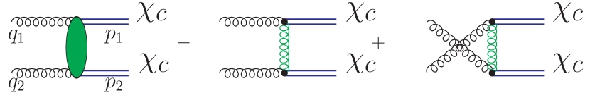
Figure 1: A diagrammatic representation of the leading order mechanisms for $pp\to\chi_{cJ_{1}}\chi_{cJ_{2}}$ reaction.

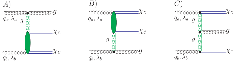
Figure 2: The lowest-order mechanisms for the $\chi_{cJ_{1}}\chi_{cJ_{2}}g$ production in the high-energy kinematics described in the text.

We are interested in three types of configurations in which a final state gluon is produced: firstly, the central production of a gluon $gg\to\chi_{cJ}\,g\,\chi_{cJ}$ (diagram (C) in Fig. 2) and secondly the two configurations with leading gluons (diagrams (A) and (B) in Fig. 2), where a gluon carries the largest fraction of momentum of one of the incoming gluons. The leading gluon minijet production is expected of importance for comparison to the $k_{T}$-factorization approach. This contribution is dominated by a kinematics, where the gluon is emitted at large rapidity distance to the $\chi_{c}$ mesons.

A gauge invariant way to organize the calculation in this situation is the use of vertices from the Lipatov effective action Lipatov:1996ts ; Antonov:2004hh .

Let us introduce the four momenta of incoming protons, neglecting their masses,

$$P_{1\mu}=\sqrt{{s\over 2}}\,n^{+}_{\mu}\,,\,P_{2\mu}=\sqrt{{s\over 2}}\,n^{-}_{\mu}\,,$$ (2)

with the lightlike basis vectors

$$n^{\pm}_{\mu}={1\over\sqrt{2}}(1,0,0,\pm 1)\,.$$ (3)

The incoming gluon momenta are

$$q_{a}=q_{a}^{+}n^{+}_{\mu}=x_{1}P_{1\mu}\,,\,q_{b}=q_{b}^{-}n^{-}_{\mu}=x_{2}P_{2\mu}\,.$$ (4)

The vertex for the “upper” leading gluon reads Lipatov:1996ts ; Antonov:2004hh

$$n^{-\rho}\,\Gamma_{\mu\nu\rho}(q_{a},p_{1})=2q^{+}_{a}g_{\mu\nu}+n^{-}_{\mu}(p_{1}-2q_{a})_{\nu}+(q_{a}-2p_{1})_{\mu}n^{-}_{\nu}-{(p_{1}-q_{a})^{2}\over q_{a}^{+}}n^{-}_{\mu}n^{-}_{\nu}\,,$$

while for the “lower” leading gluon we have

$$n^{+\rho}\Gamma_{\mu\nu\rho}(q_{b},p_{2})=2q^{-}_{b}g_{\mu\nu}+n^{+}_{\mu}(p_{2}-2q_{b})_{\nu}+(q_{b}-2p_{2})_{\mu}n^{+}_{\nu}-{(p_{2}-q_{b})^{2}\over q_{b}^{-}}n^{+}_{\mu}n^{+}_{\nu}\,.$$

For the vertex of central gluon production (the “Lipatov-vertex”) we introduce the momenta of fusing gluons

$$q_{1\mu}=q_{1}^{+}n^{+}_{\mu}+q^{\perp}_{1\mu}\,,\,q_{2\mu}=q_{2}^{-}n^{-}_{\mu}+q^{\perp}_{2\mu}\,,\,q_{i}^{2}=(q^{\perp}_{i})^{2}=-\vec{q}_{i\perp}^{2}\,.$$ (7)

So that

$$\Gamma_{\mu\rho\nu}(q_{1},q_{2}) = n^{-}_{\mu}n^{+}_{\nu}C_{\rho}(q_{1},q_{2})\,,\,$$

$$C_{\rho}(q_{1},q_{2}) = (q_{1}^{+}+{q_{1}^{2}\over q^{-}_{2}})n^{+}_{\mu}-(q_{2}^{-}+{q_{2}^{2}\over q^{+}_{1}})n^{-}_{\mu}+(q_{2}-q_{1})^{\perp}_{\mu}\,.$$ (8)

We also need the $g^{*}g^{*}\to\chi_{cJ}$ vertices. We write them in the form

$$V^{ab}_{\mu\nu}(J,J_{z};q_{1},q_{2})=-i4\pi\alpha_{S}\delta^{ab}{2R^{\prime}(0)\over\sqrt{\pi N_{c}M^{3}}}\sqrt{3}\,\cdot T_{\mu\nu}(J,J_{z};q_{1},q_{2})\,.$$ (9)

The explicit form of the tensors $T_{\mu\nu}$ are found in Ref.Cisek:2017ikn . Above $a,b$ are the color indices of incoming gluons, $N_{c}=3$ is the number of colors, and $M$ is the mass of the $\chi_{c}$ meson. For $J=1$ and $J=2$ states, the tensors have the form

$$T_{\mu\nu}(1,J_{z};q_{1},q_{2}) = T_{\mu\nu\alpha}(1;q_{1},q_{2})\varepsilon^{\alpha*}(J_{z},q_{1}+q_{2})\,,$$

$$T_{\mu\nu}(2,J_{z};q_{1},q_{2}) = T_{\mu\nu\alpha\beta}(2;q_{1},q_{2})\varepsilon^{\alpha\beta*}(J_{z},q_{1}+q_{2})\,,$$ (10)

where $\varepsilon_{\mu}(J_{z},p),\varepsilon_{\mu\nu}(J_{z},p)$ is the polarization vector/tensor for the meson with momentum $p$. The derivative of the radial wave function at the origin is related to the $\gamma\gamma$-decay width as

$$\Gamma(\chi_{c0}\to\gamma\gamma)={27e_{c}^{4}\alpha_{\rm em}^{2}\over m_{c}^{4}}|R^{\prime}(0)|^{2}\,.$$ (11)

We use the value $|R^{\prime}(0)|^{2}=0.042\,\rm{GeV}^{2}$. We can now construct all the $2\to 3$ amplitudes of interest from the above tensors. The amplitude for $gg\to\chi_{cJ_{1}}g\chi_{cJ_{2}}$ with a central gluon reads:

$${\cal M}_{C}=ig_{S}f_{a^{\prime}b^{\prime}c}\,V^{aa^{\prime}}_{1}(q_{a},p_{1}){1\over t_{1}}\,C^{\rho}(q_{a}-p_{1},q_{b}-p_{2})\varepsilon^{*}_{\rho}(\lambda_{g},p_{g})\,{1\over t_{2}}V^{bb^{\prime}}_{2}(q_{b},p_{2})\,,$$ (12)

where

$$V^{aa^{\prime}}_{1}(q_{a},p_{1}) = \varepsilon^{\mu}(\lambda_{a},q_{a})V^{aa^{\prime}}_{\mu\mu^{\prime}}(J_{1},J_{1z};q_{a},p_{1}-q_{a})n^{-\mu^{\prime}}\,,$$

$$V^{bb^{\prime}}_{2}(q_{b},p_{2}) = \varepsilon^{\nu}(\lambda_{b},q_{b})V^{bb^{\prime}}_{\nu^{\prime}\nu}(J_{2},J_{2z};q_{b},p_{2}-q_{b})n^{+\nu^{\prime}}\,.$$ (13)

The amplitude for the final state with the leading gluons in the fragmentation region of gluon $q_{a}$ or $q_{b}$ can be written in terms of the (half-) off-shell amplitude for the $g^{*}g\to\chi_{c1}\chi_{c2}$ process. The $2\to 2$ amplitude is obtained from

$${\cal M}^{ab}_{\mu\nu}(q_{a},q_{b};p_{1},p_{2}) = V^{aa^{\prime}}_{\mu\mu^{\prime}}(J_{1},J_{z1};q_{a},p_{1}-q_{a}){-g^{\mu^{\prime}\nu^{\prime}}\delta^{a^{\prime}b^{\prime}}\over\hat{t}}V^{bb^{\prime}}_{\nu^{\prime}\nu}(J_{1},J_{z1};p_{2}-q_{b},q_{b})$$

$$+V^{bb^{\prime}}_{\nu\nu^{\prime}}(J_{1},J_{z1};q_{b},p_{1}-q_{b}){-g^{\mu^{\prime}\nu^{\prime}}\delta^{a^{\prime}b^{\prime}}\over\hat{u}}V^{aa^{\prime}}_{\mu^{\prime}\mu}(J_{1},J_{z1};p_{1}-q_{a},q_{a})\,.$$

Here the Mandelstam variables are

$$\hat{t}=(p_{1}-q_{a})^{2}=(p_{2}-q_{b})^{2}\,,\,\hat{u}=(p_{1}-q_{b})^{2}=(p_{2}-q_{a})^{2}\,.$$ (15)

The amplitude of Eq. (LABEL:eq:2_to_2) enters the $2\to 3$ amplitudes as follows:

$${\cal M}_{A} = ig_{S}f_{ab^{\prime}c}\varepsilon^{\mu}(\lambda_{a},q_{a})\Gamma_{\mu\nu\rho}(q_{a},p_{g})n^{-\rho}\varepsilon^{\nu*}(\lambda_{g},p_{g}){1\over t_{1}}n^{+\mu^{\prime}}{\cal M}^{b^{\prime}b}_{\mu^{\prime}\nu^{\prime}}(p_{g}-q_{a},q_{b};p_{1},p_{2})\varepsilon^{\nu^{\prime}}(\lambda_{b},q_{b})$$ (16)

$$= ig_{S}f_{ab^{\prime}c}\,2q_{a}^{+}\delta_{\lambda_{a}\lambda_{g}}{1\over t_{1}}\,n^{+\mu^{\prime}}\varepsilon^{\nu^{\prime}}(\lambda_{b},q_{b}){\cal M}^{b^{\prime}b}_{\mu^{\prime}\nu^{\prime}}(p_{g}-q_{a},q_{b};p_{1},p_{2})\,,$$

and likewise

$${\cal M}_{B} = ig_{S}f_{a^{\prime}bc}n^{-\nu^{\prime}}\varepsilon^{\mu^{\prime}}(\lambda_{a},q_{a}){\cal M}^{aa^{\prime}}_{\mu^{\prime}\nu^{\prime}}(q_{a},p_{g}-q_{b};p_{1},p_{2})\,{1\over t_{2}}\varepsilon^{\mu}(\lambda_{b},q_{b})\Gamma_{\mu\nu\rho}(q_{b},p_{g})n^{+\rho}\varepsilon^{\nu*}(\lambda_{g},p_{g})$$ (17)

$$= ig_{S}f_{a^{\prime}bc}n^{-\nu^{\prime}}\varepsilon^{\mu^{\prime}}(\lambda_{a},q_{a}){\cal M}^{aa^{\prime}}_{\mu^{\prime}\nu^{\prime}}(q_{a},p_{g}-q_{a};p_{1},p_{2}){1\over t_{2}}\,2q_{b}^{-}\delta_{\lambda_{b}\lambda_{g}}\,.$$

We close this section with a brief comment on the gluon exchanges in the crossed channel. The $t$-channel gluons explicitly depicted in Fig.2 are taken in the respective high-energy limit - they correspond to the reggeized gluons of the effective action Antonov:2004hh ; Lipatov:1996ts . For the gluon exchanges in the blobs of diagrams (A) and (B) of Fig.2 we checked that the approximation of reggeized gluon exchange in the $gg\to\chi_{c}\chi_{c}$ subprocess becomes a good approximation at a rapidity distance between $\chi_{c}$’s of $\Delta y\gtrapprox 3$. In the numerical calculations, we use the full gluon propagator in Feynman-gauge. We note that the interference between $t$- and $u$-channel amplitudes is negligible and confined to a very narrow interval around $\Delta y\sim 0$.

II.2 Parton-level cross sections

Let us now have a look at the parton-level cross section in order to understand better the kinematics and possible singularities in the integration over phase space. The $2\to 3$ parton-level cross sections are obtained from

$$d\sigma={1\over 4q_{a}^{+}q_{b}^{-}}\,|\overline{{\cal M}_{i}}|^{2}\,d\Phi(q_{a}+q_{b};p_{1},p_{2},p_{g})\,,$$ (18)

where $i=A,B,C$, and there is no interference between the diagrams of Fig.2. Let us start from the production of a leading gluon along the direction of incoming gluon $a$, described by amplitude ${\cal M}_{A}$. Here, following the rules of the high-energy limit, the four-momentum $q_{1}\equiv p_{g}-q_{a}$ of the exchanged gluon enters the $2\to 2$ amplitude in the form

$$q_{1\mu}=q^{+}_{1}n^{+}_{\mu}+q^{\perp}_{1\mu}\equiv z_{1}q^{+}_{a}n^{+}_{\mu}+q_{1\perp}e^{\perp}_{\mu}\,.$$ (19)

We can now use the Ward-identity, to write

$$n^{+\mu}\varepsilon^{\nu}(\lambda_{b},q_{b}){\cal M}^{b^{\prime}b}_{\mu\nu}(q_{1},q_{b};p_{1},p_{2}) = {q_{1\perp}\over q^{+}_{1}}e^{\perp\mu}\varepsilon^{\nu}(\lambda_{b},q_{b}){\cal M}^{b^{\prime}b}_{\mu\nu}(q_{1},q_{b};p_{1},p_{2})$$ (20)

$$\equiv {q_{1\perp}\over q^{+}_{1}}{\cal M}(2\to 2)\,.$$

Then, the $2\to 3$ cross section takes the simple form

$$d\sigma(2\to 3) = {2C_{A}\alpha_{S}\over\pi}{q^{2}_{1\perp}\over t_{1}^{2}}{d^{2}\vec{q}_{1\perp}\over\pi}{dz_{1}\over z_{1}(1-z_{1})}\,{1\over 4q_{1}^{+}q_{b}^{-}}|\overline{{\cal M}(2\to 2)}|^{2}\,d\Phi(q_{1}+q_{b};p_{1},p_{2})$$ (21)

$$= {2C_{A}\alpha_{S}\over\pi}{d^{2}\vec{q}_{1\perp}\over\pi q^{2}_{1\perp}}{dz_{1}\over z_{1}}\,\cdot{1\over 2q_{1}^{+}q_{b}^{-}}|\overline{{\cal M}(2\to 2)}|^{2}\,d\Phi(q_{1}+q_{b};p_{1},p_{2})\,.$$

Here one would recognized the factorization in the unintegrated gluon distribution in a gluon

$${zdn_{g/g}(z,\vec{q}_{\perp})\over dzd\log q_{\perp}^{2}}={2C_{A}\alpha_{S}\over\pi}\,,$$ (22)

and the off-shell cross section for the process $g^{*}g\to\chi_{c}\chi_{c}$. The off-shell cross section will provide us with a scale $\mu^{2}\sim M^{2}_{\perp}$, so that for $q_{1\perp}^{2}\ll\mu^{2}$ we can neglect the off-shellness of gluon $q_{1}$ and only the on shell cross section $gg\to\chi_{c}\chi_{c}$ enters. The parton-level cross section then consists of two parts:

$$d\sigma(2\to 3)={2C_{A}\alpha_{S}\over\pi}\int^{\mu^{2}}{dq^{2}_{1\perp}\over q^{2}_{1\perp}}{dz_{1}\over z_{1}}\,d\sigma(2\to 2)+{2C_{A}\alpha_{S}\over\pi}\int_{\mu^{2}}{d^{2}\vec{q}_{1\perp}\over\pi q^{2}_{1\perp}}{dz_{1}\over z_{1}}d\sigma(2\to 2;\vec{q}_{1\perp})$$

Here the first piece contains the infrared divergent integral $\int^{\mu^{2}}dq^{2}_{1\perp}/q^{2}_{1\perp}$, which is of course just the collinear logarithm in the $g\to gg$ splitting. In a complete NLO calculation of the inclusive $\chi_{c}\chi_{c}$ the collinear logarithm within some factorization scheme would be absorbed into the evolution of the gluon distribution of one of the protons. The contribution from hard $q^{2}_{\perp 1}>\mu^{2}$ is a genuine NLO contribution. In our numerical calculations we will simply show the $2\to 3$ cross section with a lower cutoff on the transverse momentum of the produced gluon (mini-)jet, $p_{g\perp}>p^{\rm cut}_{g\perp}\sim 1\,\rm{GeV}$.

Let us now come to the contribution from production of a central gluon in the $gg\to\chi_{c}g\chi_{c}$ process. We write the parton-level cross section differential in the gluon rapdity $y_{g}$ and the transverse momenta of $\chi_{c}$ mesons $\vec{p}_{1,2\perp}$.

$${d\sigma(gg\to\chi_{c}g\chi_{c})}={1\over 256\pi^{5}\hat{s}^{2}}|\overline{{\cal M}_{C}}|^{2}\,dy_{g}d^{2}\vec{p}_{1\perp}d^{2}\vec{p}_{2\perp}\,.$$ (24)

The square of the amplitude ${\cal M}_{C}$ of Eq.(12) can be written in the usual impact factor representation

$$\overline{|{\cal M}_{C}|^{2}} = {N_{c}\over N_{c}^{2}-1}16\pi\alpha_{S}\,I_{1}(\vec{p}_{1\perp}){\hat{s}^{2}\over(\vec{p}_{1\perp}+\vec{p}_{2\perp})^{2}}I_{2}(\vec{p}_{2\perp})\,$$

$$= {16\pi^{3}\hat{s}^{2}\over N_{c}^{2}-1}I_{1}(\vec{p}_{1\perp}){\cal K}_{r}(\vec{p}_{1\perp},-\vec{p}_{2\perp})I_{2}(\vec{p}_{2\perp})\,.$$

Here ${\cal K}_{r}$ is the real-emission part of the BFKL-kernel BFKL

$${\cal K}_{r}(\vec{p}_{1\perp},-\vec{p}_{2\perp})={C_{A}\alpha_{S}\over\pi^{2}}{1\over(\vec{p}_{1\perp}+\vec{p}_{2\perp})^{2}}\,.$$ (26)

Notice that the integral over the gluon rapidity is proportional to $Y=\log(\hat{s}/M^{2})$, so that the $2\to 3$ cross section will be

$$d\sigma(2\to 3)={Y\over 16\pi^{2}(N_{c}^{2}-1)}\,I_{1}(\vec{p}_{1\perp}){\cal K}_{r}(\vec{p}_{1\perp},-\vec{p}_{2\perp})I_{2}(\vec{p}_{2\perp})d^{2}\vec{p}_{1\perp}d^{2}\vec{p}_{2\perp}\,.$$ (27)

Here we again have an infrared singularity when $\vec{p}_{g\perp}=-\vec{p}_{1\perp}-\vec{p}_{2\perp}\to 0$. This is of course just the back-to-back region of the $2\to 2$ process. The differential cross section of the Born-level $2\to 2$ cross section can be expressed in terms of the same impact factors and reads

$$d\sigma^{(0)}(2\to 2)={1\over 16\pi^{2}(N_{c}^{2}-1)}I_{1}(\vec{p}_{1\perp})\delta^{(2)}(\vec{p}_{1\perp}+\vec{p}_{2\perp})I_{2}(\vec{p}_{2\perp})d^{2}\vec{p}_{1\perp}d^{2}\vec{p}_{2\perp}\,.$$ (28)

To the leading order in $\alpha_{S}Y$, the virtual correction to the $2\to 2$ process can be easily calculated using the gluon reggeization property, which amounts to the replacement of the gluon propagator by

$${1\over q^{2}}\to{1\over q^{2}}\,\exp[\omega(\vec{q}_{\perp})Y]\,,$$ (29)

where

$$\omega(\vec{q}_{\perp})=-{\alpha_{S}N_{c}\over 4\pi^{2}}\int d^{2}\vec{Q}_{\perp}{\vec{q}^{2}_{\perp}\over\vec{Q}^{2}_{\perp}(\vec{Q}_{\perp}-\vec{q}_{\perp})^{2}}\,.$$ (30)

Expanding the Regge-propagator to the first order, we obtain the $2\to 2$ process cross section as

$$d\sigma(2\to 2) = d\sigma^{(0)}(2\to 2)$$

$$+ {Y\over 16\pi^{2}(N_{c}^{2}-1)}I_{1}(\vec{p}_{1\perp})\delta^{(2)}(\vec{p}_{1\perp}+\vec{p}_{2\perp})2\omega(\vec{p}_{1\perp})I_{2}(\vec{p}_{2\perp})d^{2}\vec{p}_{1\perp}d^{2}\vec{p}_{2\perp}\,.$$

Then, the inclusive cross section for the production of $\chi_{c}$-pairs becomes

$$d\sigma(gg\to\chi_{c}\chi_{c}X)=d\sigma^{(0)}+{Y\over 16\pi^{2}(N_{c}^{2}-1)}I_{1}(\vec{p}_{1\perp}){\cal K}_{\rm BFKL}(\vec{p}_{1\perp},-\vec{p}_{2\perp})I_{2}(\vec{p}_{2\perp})d^{2}\vec{p}_{1\perp}d^{2}\vec{p}_{2\perp}\,.$$

Here ${\cal K}_{\rm BFKL}$ is the leading-order in $\alpha_{S}Y$ BFKL kernel

$${\cal K}_{\rm BFKL}(\vec{p}_{1\perp},-\vec{p}_{2\perp}) = {\cal K}_{r}(\vec{p}_{1\perp},-\vec{p}_{2\perp})+{\cal K}_{\rm v}(\vec{p}_{1\perp},-\vec{p}_{2\perp})$$

$$= {\alpha_{S}N_{c}\over\pi^{2}}\Big{(}{1\over(\vec{q}_{1\perp}+\vec{q}_{2\perp})^{2}}-\delta^{(2)}(\vec{q}_{1\perp}+\vec{q}_{2\perp}){1\over 2}\int d^{2}{\vec{Q}}_{\perp}{\vec{q}^{2}_{\perp}\over\vec{Q}^{2}_{\perp}(\vec{Q}_{\perp}-\vec{q}_{\perp})^{2}}\Big{)}\,.$$

We cannot absorb the infrared divergencies into the initial state parton distributions in this case. However, for the sufficiently inclusive, say over soft gluon radiation, cross section, the infrared divergencies in the real and virtual part of the BFKL-kernel will cancel. Notice that this mechanism resembles in many respects the Mueller-Navelet dijet production Mueller:1986ey , with the $\chi_{c}$ playing the role of the jets. However, for this case more involved calculations including a full BFKL-resummation have been performed in recent years Ducloue:2013bva ; Caporale:2014gpa . As in the case for production of leading gluons, we will in our numerical calculations show the contribution from the $\chi_{c}\chi_{c}g$ final state with a lower cutoff on the transverse momentum of the gluon $p_{g\perp}=|\vec{q}_{1\perp}+\vec{q}_{2\perp}|>p^{\rm cut}_{g\perp}\sim 1\,\rm{GeV}$.

II.3 Hadron-level cross sections

We now come to the hadron-level cross sections. Below $s$ is the proton-proton center-of-mass energy squared. The inclusive production of $\chi_{c}$-pairs from the $2\to 2$ process is obtained from

$$\displaystyle d\sigma = x_{1}g(x_{1},\mu^{2})x_{2}g(x_{2},\mu^{2}){1\over 16\pi(x_{1}x_{2}s)^{2}}|\overline{\mathcal{M}(2\to 2)}|^{2}dy_{1}dy_{2}d^{2}\vec{p}_{1\perp}d^{2}\vec{p}_{2\perp}\delta^{(2)}(\vec{p}_{1\perp}+\vec{p}_{2\perp})\,,$$

with $p_{T}=|\vec{p}_{1\perp}|$, and

$$x_{1}=\sqrt{{M^{2}+p_{T}^{2}\over s}}\Big{(}e^{y_{1}}+e^{y_{2}}\Big{)}\,,\,x_{2}=\sqrt{{M^{2}+p_{T}^{2}\over s}}\Big{(}e^{-y_{1}}+e^{-y_{2}}\Big{)}\,.$$ (35)

The cross section for the $2\to 3$ processes is calculated from:

$$d\sigma = x_{1}g(x_{1},\mu^{2})x_{2}g(x_{2},\mu^{2}){1\over 256\pi^{5}(x_{1}x_{2}s)^{2}}|\overline{\mathcal{M}(2\to 3)}|^{2}$$ (36)

$$\times dy_{1}dy_{2}dy_{g}d^{2}\vec{p}_{1\perp}d^{2}\vec{p}_{2\perp}d^{2}\vec{p}_{g\perp}\delta^{(2)}(\vec{p}_{1\perp}+\vec{p}_{2\perp}+\vec{p}_{g\perp})$$

with

$$\displaystyle x_{1} = \frac{m_{1\perp}}{\sqrt{s}}e^{y_{1}}+\frac{m_{2\perp}}{\sqrt{s}}e^{y_{2}}+\frac{p_{g\perp}}{\sqrt{s}}e^{y_{g}}\,,$$ (37)

$$x_{2} = \frac{m_{1\perp}}{\sqrt{s}}e^{-y_{1}}+\frac{m_{2\perp}}{\sqrt{s}}e^{-y_{2}}+\frac{p_{g\perp}}{\sqrt{s}}e^{-y_{g}}\,,$$ (38)

where $m_{i\perp}=\sqrt{M^{2}+p_{i\perp}^{2}}$ and $y_{1,2}$ are the cm-rapidities of mesons. We take as the factorization scale $\mu^{2}=\hat{s}=x_{1}x_{2}s$. For the case of identical $\chi_{c}$-mesons in the final state all of the cross sections must be multiplied by $1/2$.

III Numerical Results

III.1 Parton level processes

In this subsection we show two examples of rapidity distributions on the parton level for the process (C) in Fig.2.

In Fig.3 we show distribution in rapidity for the $gg\to\chi_{c0}g\chi_{c0}$. Here the center of mass energy has been fixed at $W$ = 50 GeV. The two $\chi_{c0}$ mesons are produced in forward and backward directions while gluon at midrapidity in the partonic center-of-mass system. For comparison we show also rapidity distributions of $\chi_{c0}$ mesons from the $gg\to\chi_{c0}\chi_{c0}$ process (solid line).

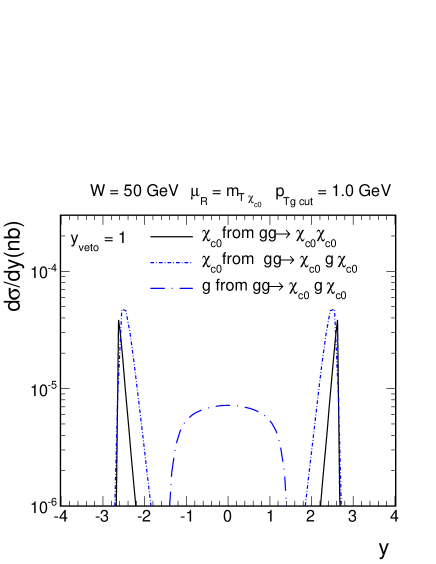
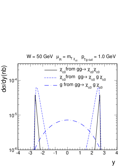
Figure 3: Differential cross section for the processes from Fig.1 and Fig.2 (C) at the parton level, where the energy in the center of mass of two gluons was fixed for $W=50\>\rm{GeV}$. The left panel is for extra rapidity veto and the right panel without the extra condition.

Similar distribution for the $gg\to\chi_{c1}g\chi_{c1}$ process is shown in Fig.4. The situation is similar as for the $\chi_{c0}\chi_{c0}$ pair production. However, the $2\to 3$ contribution here is relatively enhanced compared to the $2\to 2$ one (solid lines). In each of the $gg\rightarrow\chi_{c1}$ vertices in the $2\rightarrow 2$ process only one gluon is off-mass-shell, whereas in the $2\rightarrow 3$ process in one of the vertices both gluons are off-mass-shell. The vertex $g^{*}g^{*}\rightarrow\chi_{c1}$ strongly depends on virtualities of the gluons. We remind that when gluons are on-mass-shell the vertex vanishes (Landau-Yang theorem Landau-Yang ).

To ensure validity of the effective Regge action (applicability of the Lipatov-vertex) one should ensure that the gluon is produced at a distance of at least $y_{\rm veto}\sim 1$ from the mesons. We therefore show in the left panels of Figs. 3,4 the result obtained for $y_{\rm veto}=1$ and in the right panels the result without a rapidity veto. Interestingly, for the $\chi_{c0}$ case, the gluon is automatically produced centrally, while for the case of $\chi_{c1}$ production the rapidity veto is important to exclude contributions from non-central kinematics.

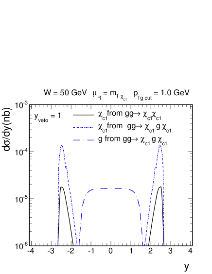
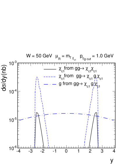
Figure 4: Differential cross section for the processes from Fig.1 and Fig.2 (C) at the parton level, where the energy in the center of mass of two gluons was fixed for $W=50\>\rm{GeV}$. The left panel is for extra rapidity veto and the right panel without the extra condition.

III.2 Hadron level cross sections

The integrated cross sections (full phase space) for different components are shown in Table 1 for $\sqrt{s}=8\,\rm{TeV}$. We restrict ourselves to the case of “identical” pairs, i.e. $\chi_{c0}\chi_{c0}$, $\chi_{c1}\chi_{c1}$, or $\chi_{c2}\chi_{c2}$. We see, that the cross sections for the $2\to 2$ processes are consistently lower than the ones obtained in the $k_{T}$-factorization approach in Ref. Cisek:2017ikn .

Table 1: Values of total cross sections for particular processes for $\sqrt{s}=8\,\rm{TeV}$.

$\chi_{c2}$	$\sigma_{\rm total}$	$\chi_{c1}$	$\sigma_{\rm total}$	$\chi_{c0}$	$\sigma_{\rm total}$
$pp\rightarrow\chi_{c2}\chi_{c2}$	$0.62\,\rm{nb}$	$pp\rightarrow\chi_{c1}\chi_{c1}$	$8.60\cdot 10^{-2}\,\rm{nb}$	$pp\rightarrow\chi_{c0}\chi_{c0}$	$0.40\,\rm{nb}$
$pp\rightarrow[\chi_{c2}\chi_{c2}]g$	$0.19\,\rm{nb}\times 2$	$pp\rightarrow[\chi_{c1}\chi_{c1}]g$	$4.07\cdot 10^{-2}\,\rm{nb}\times 2$	$pp\rightarrow[\chi_{c0}\chi_{c0}]g$	$0.10\,\rm{nb}\times 2$
$pp\rightarrow\chi_{c2}g\chi_{c2}$	$0.16\,\rm{nb}$	$pp\rightarrow\chi_{c1}g\chi_{c1}$	$1.78\cdot 10^{-2}\,\rm{nb}$	$pp\rightarrow\chi_{c0}g\chi_{c0}$	$0.03\,\rm{nb}$

In Fig.5 we show transverse momentum distribution of one of the $\chi_{c}$ mesons for the $2\to 2$ and $2\to 3$ processes. The $2\to 3$ contributions were calculated with $p_{Tg}>1\,\rm{GeV}$. The factorization scale is chosen as $\mu_{f}=\sqrt{\hat{s}}$ and the energy in the center of mass of two protons is $8\>\rm{TeV}$. We use the $MSTW2008nlo$ MSTW parton distribution functions. For illustration in a few plots we present only diagram (B) from Fig.2, since the behaviour of the process described by diagram (A) is exactly opposite. We discuss pairs, where two of $\chi_{c}^{\prime}s$ have the same spin, it is good example to show all characteristics of these mesons. Notice, that in high transverse momentum region, the $pp\rightarrow[\chi_{c}\chi_{c}]g$ process dominates for each $\chi_{cJ}$, though for $\chi_{c1}$ it is not big effect.

In Fig.6 we show rapidity distributions of $\chi_{c}$ mesons for the different $2\to 2$ and $2\to 3$ mechanisms discussed above. One can see that in the rapidity range $|y|>3$ the $pp\rightarrow[\chi_{c1}\chi_{c1}]g$ process is not negligible (the middle plot in Fig.6). While the $2\to 2$ sub-processes lead to the production of $\chi_{c}$ mesons at midrapidities the $2\to 3$ processes generate $\chi_{c}$ mesons also at large $|y|$. Such mesons are then suppressed in the midrapidity experiments as ATLAS or CMS. The same may be true in the case of forward LHCb experiment. When the forward emitted meson is measured the second meson is emitted preferentially at midrapidities (diagrams (A) and (B)) or even in opposite directions (diagram (C)). We leave detailed studies relevant for a given experiment for the future.

In Fig.7 we compare rapidity distributions of $\chi_{c}$ mesons and the associated gluon (see diagram (C) in Fig.2). In this case, while the $\chi_{c}$ quarkonia are produced preferentially in forward or backward directions, gluons are emitted preferentially at midrapidities. For comparison we show also distributions of $\chi_{c}$ quarkonia from the $2\to 2$ sub-processes.

In Fig.8 we show similar distributions for diagrams (A) and (B) in Fig.2 and for reference also the distributions from the $2\to 2$ sub-processes.

In general, there is rapidity ordering of final state particles for the considered $2\to 3$ processes. To see it even better let us present now distributions in rapidity differences between final state objects.

The distribution in rapidity distance between two $\chi_{c}$ mesons is shown in Fig.9 for different components discussed in the present paper: $\chi_{c0}\chi_{c0}$, $\chi_{c1}\chi_{c1}$ and $\chi_{c2}\chi_{c2}$. Indeed, as expected, the largest distances between the $\chi_{c}$ quarkonia are populated by processes with the gluon emitted among both $\chi_{c}$ mesons. Then also a sizeable gap at small rapidity distances can be observed.

In Fig.10 we show similar distributions, this time for rapidity distance between one of the $\chi_{c}$ mesons and the associated gluon for $\chi_{c0}\chi_{c0}$, $\chi_{c1}\chi_{c1}$ and $\chi_{c2}\chi_{c2}$. The considered mechanisms prefer large distances also in this variable.

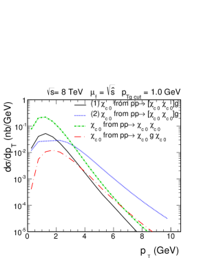
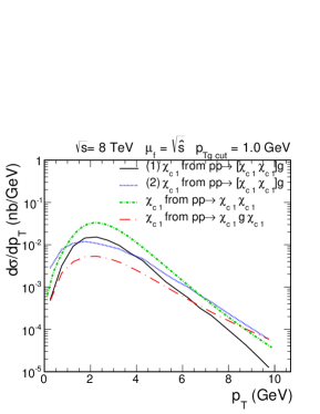
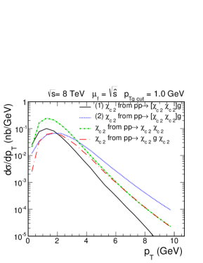
Figure 5: Transverse momenta distributions of one of the $\chi_{c}$ for the $pp\to\chi_{cJ}\chi_{cJ}$ and $pp\to\chi_{cJ}\chi_{cJ}g$ reaction for $\sqrt{s}=8\>TeV$.

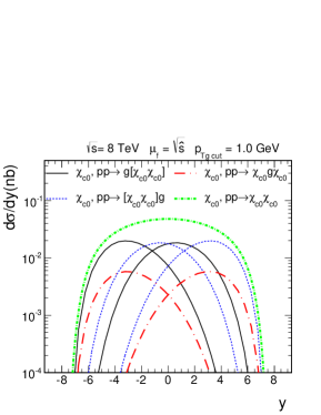
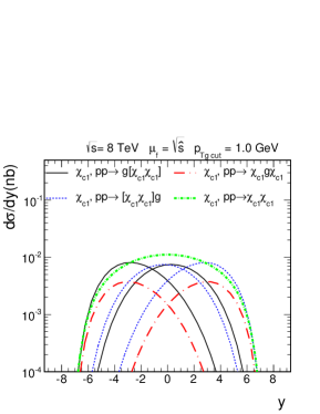
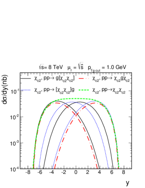
Figure 6: Rapidity distributions of $\chi_{c}$ mesons from $2\to 2$ and $2\to 3$ processes shown in Fig.2 for $\chi_{c0}\chi_{c0}$ (left) and $\chi_{c1}\chi_{c1}$ (middle) and $\chi_{c2}\chi_{c2}$ (right). Here $\mu_{f}^{2}=\hat{s}$ was used.

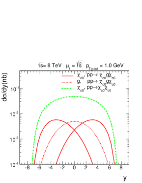
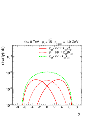
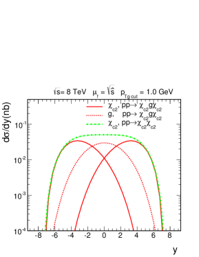
Figure 7: Rapidity distributions of $\chi_{c}$ mesons and gluons from the $gg\to\chi g\chi$ processes with a central gluon. Here $\mu_{f}^{2}=\hat{s}$ was used.

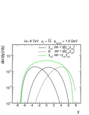
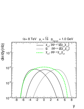
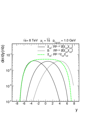
Figure 8: Rapidity distributions of $\chi_{c}$ mesons and gluons from the $gg\to g\chi_{c}\chi_{c}$ processes with a leading gluon. Here $\mu_{f}^{2}=\hat{s}$ was used.

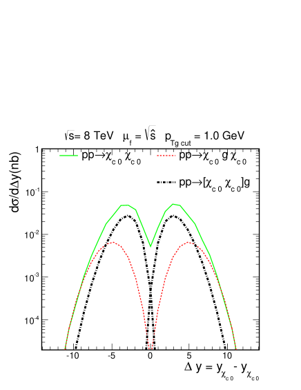
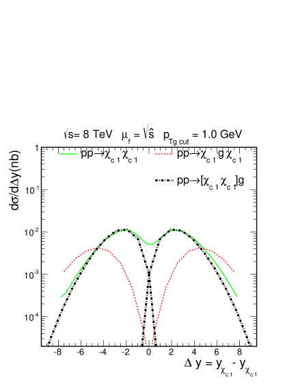
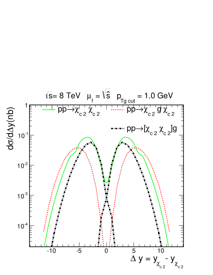
Figure 9: Distribution in the difference of rapidities of $\chi_{cJ}$ mesons from processes shown in diagrams [2]. The most external lines are from process, where gluon is emitted among the two $\chi_{cJ}$ mesons.

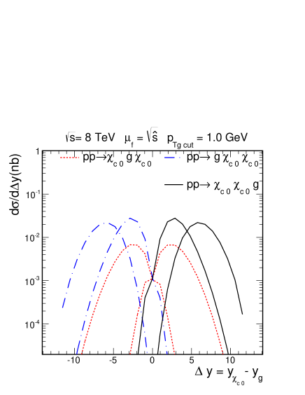
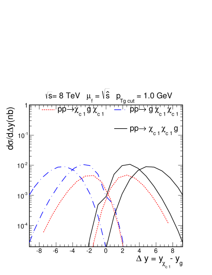
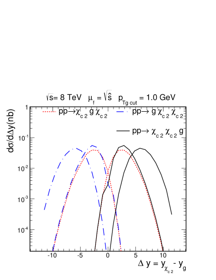
Figure 10: Distribution in the difference of rapidities between $\chi_{cJ}$ meson and gluon from diagrams presented in Fig.2. The most external lines in the plot are for difference between external gluon and the external $\chi_{cJ}$ meson (diagram (A) and (B) from Fig. 2 ).

Let us discuss now some correlation observables.

In Fig.11 -13 we show two-dimensional distributions in transverse momenta of both $\chi_{c}$ quarkonia for separate ((A) or (B) in Fig. 2) diagrams. Such separation is possible due to quite different phase space population of the different mechanisms (diagrams).

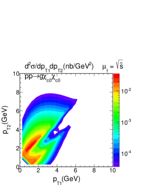
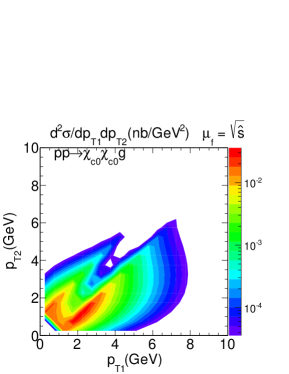
Figure 11: Two-dimensional distributions ($p_{T1}\times p_{T2}$) for $\chi_{c0}\chi_{c0}$ production. Here $\mu_{f}^{2}=\hat{s}$.

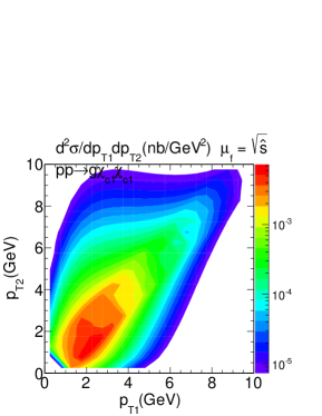
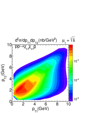
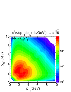
Figure 12: Two-dimensional distributions ($p_{T1}\times p_{T2}$) for $\chi_{c1}\chi_{c1}$ production. Here $\mu_{f}^{2}=\hat{s}$.

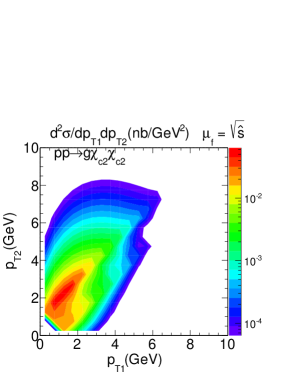
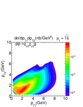
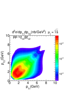
Figure 13: Two-dimensional distributions ($p_{T1}\times p_{T2}$) for $\chi_{c2}\chi_{c2}$ production. Here $\mu_{f}^{2}=\hat{s}$.

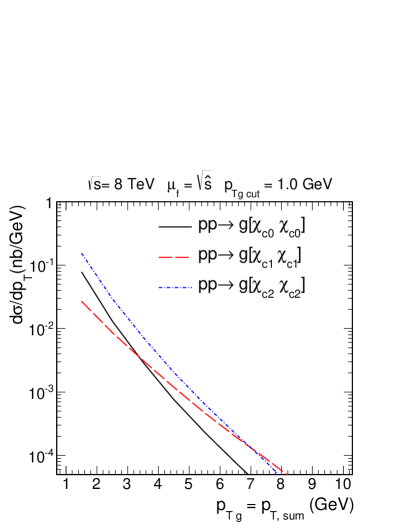
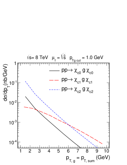
Figure 14: Distribution in $\vec{p}_{T,sum}$, where $\vec{p}_{T,sum}=\vec{p}_{1T}+\vec{p}_{2T}$ for $pp\rightarrow g[\chi_{cJ}\chi_{cJ}]$ (the left panel) and $pp\rightarrow\chi_{cJ}g\chi_{cJ}$ (the right panel) processes for $\sqrt{s}=8\>\rm{TeV}$. Here $\mu_{f}^{2}=\hat{s}$.

Finally in Fig.14 we show distribution in $p_{T,sum}$ (vector sum of transverse momenta of both outgoing quarkonia) for different involved contributions. Because of the momentum conservation it equals the transverse-momentum distribution of the emitted gluon. A significant difference between diagram (A) and (B) or (C) appears for $\chi_{c1}$. Emission of the gluon is suppressed in diagram (A) at small $p_{T}$ region. While the distributions for $\chi_{c0}\chi_{c0}$ and $\chi_{c2}\chi_{c2}$ are similar, the distributions for $\chi_{c1}\chi_{c1}$ are clearly less steep. Similar observation was already made in the $k_{T}$-factorization study in Cisek:2017ikn . This is particularly spectacular for the central emission diagram (diagram (C) in Fig.2) when both gluons are off-mass-shell.

IV Conclusions

In the present paper we have calculated differential cross sections for $\chi_{c}$ pair production in the collinear approach including next-to-leading order corrections ($2\to 3$ processes). Here we have considered only symmetric pairs (identical $\chi_{c}$ mesons). The present results can be compared to previously calculated cross sections in the $k_{T}$-factorization approach with the KMR unintegrated gluon distributions. We have found that the leading-order $2\to 2$ processes give much smaller cross sections than those in the $k_{T}$-factorization approach. Therefore we have calculated higher-order corrections including $2\to 3$ processes. There are three typical diagrams with emission of leading and central gluons (see Fig.2). The cross section for leading gluon emission is much larger.

When adding the leading and (real emission part of the) next-to-leading order contribution we have obtained results that are similar to the $k_{T}$-factorization results for the production of $\chi_{c0}\chi_{c0}$ and $\chi_{c2}\chi_{c2}$ but still considerably less than in the $k_{T}$-factorization approach for the $\chi_{c1}\chi_{c1}$. The latter disagreement is likely due to even higher-order (NNLO) contributions (involving $2\to 4$ processes) contained effectively in the $k_{T}$-factorisation which may be crucial to include for the $\chi_{c1}\chi_{c1}$ channel as here the vertices vanish for on-shell gluons. In general, the larger numerical value of deviation from the on-shell situation the larger the vertex. We expect that consistent inclusion of the NNLO corrections may be important in this particular case and much less important for other cases. A detailed study will be done elsewhere.

The central gluon emission is interesting in that it enhances production of $\chi_{c}$’s at large rapidity distances. This is similar to the Mueller-Navelet production of large rapidity distance dijets and one may think of a larger enhancement from resummation.

We have calculated several single-particle differential distributions in rapidity and transverse momentum of $\chi_{c}$ mesons as well as some correlation observables such as two-dimensional distribution in transverse momenta of both $\chi_{c}$ quarkonia or in transverse momentum of the quarkonium pair.

Acknowledgments

This study was partially supported by the Polish National Science Center grant DEC- 2014/15/B/ST2/02528 and by the Center for Innovation and Transfer of Natural Sciences and Engineering Knowledge in Rzeszów.

References

- (1) N. Brambilla et al., Eur. Phys. J. C 71 (2011) 1534 [arXiv:1010.5827 [hep-ph]].
- (2) B. Gong, X. Q. Li and J. X. Wang, Phys. Lett. B 673, 197 (2009) Erratum: [Phys. Lett. B 693, 612 (2010)] [arXiv:0805.4751 [hep-ph]].
- (3) J. M. Campbell, F. Maltoni and F. Tramontano, Phys. Rev. Lett. 98, 252002 (2007) [hep-ph/0703113 [HEP-PH]].
- (4) J. P. Lansberg, Phys. Lett. B 695, 149 (2011) [arXiv:1003.4319 [hep-ph]].
-
(5)
S. Catani, M. Ciafaloni and F. Hautmann,
Nucl. Phys. B 366, 135 (1991);
J. C. Collins and R. K. Ellis,
Nucl. Phys. B 360, 3 (1991);
E. M. Levin, M. G. Ryskin, Y. M. Shabelski and A. G. Shuvaev, Sov. J. Nucl. Phys. 53, 657 (1991) [Yad. Fiz. 53, 1059 (1991)]. - (6) M. A. Kimber, A. D. Martin and M. G. Ryskin, Phys. Rev. D 63, 114027 (2001) [hep-ph/0101348].
- (7) S. P. Baranov, A. V. Lipatov and N. P. Zotov, Phys. Rev. D 93, no. 9, 094012 (2016) [arXiv:1510.02411 [hep-ph]].
- (8) B. A. Kniehl, D. V. Vasin and V. A. Saleev, Phys. Rev. D 73, 074022 (2006) [hep-ph/0602179].
- (9) S. P. Baranov, Phys. Rev. D 66, 114003 (2002).
- (10) S. P. Baranov and A. Szczurek, Phys. Rev. D 77, 054016 (2008) [arXiv:0710.1792 [hep-ph]].
- (11) A. Cisek and A. Szczurek, Phys. Rev. D 97, no. 3, 034035 (2018) [arXiv:1712.07943 [hep-ph]].
- (12) V. M. Abazov et al. [D0 Collaboration], Phys. Rev. D 90, no. 11, 111101 (2014) [arXiv:1406.2380 [hep-ex]].
- (13) R. Aaij et al. [LHCb Collaboration], Phys. Lett. B 707, 52 (2012) [arXiv:1109.0963 [hep-ex]].
- (14) V. Khachatryan et al. [CMS Collaboration], JHEP 1409, 094 (2014) [arXiv:1406.0484 [hep-ex]].
- (15) R. Aaij et al. [LHCb Collaboration], JHEP 1706, 047 (2017) Erratum: [JHEP 1710, 068 (2017)] [arXiv:1612.07451 [hep-ex]].
- (16) M. Aaboud et al. [ATLAS Collaboration], Eur. Phys. J. C 77, no. 2, 76 (2017) [arXiv:1612.02950 [hep-ex]].
- (17) C. H. Kom, A. Kulesza and W. J. Stirling, Phys. Rev. Lett. 107, 082002 (2011) [arXiv:1105.4186 [hep-ph]].
- (18) M. Luszczak, R. Maciula and A. Szczurek, Phys. Rev. D 85, 094034 (2012) [arXiv:1111.3255 [hep-ph]].
-
(19)
F. Abe et al. [CDF Collaboration],
Phys. Rev. Lett. 79, 584 (1997)
F. Abe et al. [CDF Collaboration], Phys. Rev. D 56, 3811 (1997);
V. M. Abazov et al. [D0 Collaboration], Phys. Rev. D 81, 052012 (2010) [arXiv:0912.5104 [hep-ex]]; G. Aad et al. [ATLAS Collaboration], New J. Phys. 15, 033038 (2013) [arXiv:1301.6872 [hep-ex]]; S. Chatrchyan et al. [CMS Collaboration], JHEP 1403, 032 (2014) [arXiv:1312.5729 [hep-ex]]; G. Aad et al. [ATLAS Collaboration], JHEP 1404, 172 (2014) [arXiv:1401.2831 [hep-ex]]; R. Aaij et al. [LHCb Collaboration], JHEP 1206, 141 (2012) Addendum: [JHEP 1403, 108 (2014)] [arXiv:1205.0975 [hep-ex]]. - (20) A. Cisek, W. Schäfer and A. Szczurek, Phys. Rev. D 97, no. 11, 114018 (2018) [arXiv:1711.07366 [hep-ph]].
- (21) S. P. Baranov, Phys. Atom. Nucl. 60, 986 (1997) [Yad. Fiz. 60, 1103 (1997)].
- (22) A. K. Likhoded, A. V. Luchinsky and S. V. Poslavsky, Phys. Rev. D 94, no. 5, 054017 (2016) [arXiv:1606.06767 [hep-ph]].
- (23) L. N. Lipatov, Phys. Rept. 286, 131 (1997) [hep-ph/9610276].
- (24) E. N. Antonov, L. N. Lipatov, E. A. Kuraev and I. O. Cherednikov, Nucl. Phys. B 721, 111 (2005) [hep-ph/0411185].
- (25) V. S. Fadin, E. A. Kuraev and L. N. Lipatov, Phys. Lett. 60B, 50 (1975); E. A. Kuraev, L. N. Lipatov and V. S. Fadin, Sov. Phys. JETP 45, 199 (1977) [Zh. Eksp. Teor. Fiz. 72, 377 (1977)]; I. I. Balitsky and L. N. Lipatov, Sov. J. Nucl. Phys. 28, 822 (1978) [Yad. Fiz. 28, 1597 (1978)].
- (26) A. H. Mueller and H. Navelet, Nucl. Phys. B 282, 727 (1987).
- (27) F. Caporale, D. Y. Ivanov, B. Murdaca and A. Papa, Eur. Phys. J. C 74, no. 10, 3084 (2014) Erratum: [Eur. Phys. J. C 75, no. 11, 535 (2015)] [arXiv:1407.8431 [hep-ph]].
- (28) B. Ducloué, L. Szymanowski and S. Wallon, Phys. Rev. Lett. 112, 082003 (2014) [arXiv:1309.3229 [hep-ph]].
-
(29)
L. D. Landau,
Dokl. Akad. Nauk Ser. Fiz. 60, no. 2, 207 (1948);
C. N. Yang, Phys. Rev. 77, 242 (1950). - (30) A. D. Martin, W. J. Stirling, R. S. Thorne and G. Watt, Eur. Phys. J. C 63, 189 (2009) [arXiv:0901.0002 [hep-ph]].