Manifold valued data analysis of samples of networks, with applications in corpus linguistics

Abstract

Networks arise in many applications, such as in the analysis of text documents, social interactions and brain activity. We develop a general framework for extrinsic statistical analysis of samples of networks, motivated by networks representing text documents in corpus linguistics. We identify networks with their graph Laplacian matrices, for which we define metrics, embeddings, tangent spaces, and a projection from Euclidean space to the space of graph Laplacians. This framework provides a way of computing means, performing principal component analysis and regression, and carrying out hypothesis tests, such as for testing for equality of means between two samples of networks. We apply the methodology to the set of novels by Jane Austen and Charles Dickens.

T1This work was supported by the Engineering and Physical Sciences Research Council [grant number EP/T003928/1 and EP/M02315X/1]. The authors are grateful to Michaela Mahlberg, Viola Wiegand and Anthony Hennessey for their help and discussions about the data, and to the Editor, Associate Editor and two anonymous referees for their very helpful comments.

and

1 Introduction

The statistical analysis of networks dates back to at least the 1930’s, however interest has increased considerably in the 21st century (Kolaczyk, 2009). Networks are able to represent many different types of data, for example social networks, neuroimaging data and text documents. In this paper, each observation is a weighted network, denoted $G_{m}=(V,E)$, comprising a set of nodes, $V=\{v_{1},v_{2},\ldots,v_{m}\}$, and a set of edge weights, $E=\{w_{ij}:w_{ij}\geq 0,1\leq i,j\leq m\}$, indicating nodes $v_{i}$ and $v_{j}$ are either connected by an edge of weight $w_{ij}>0$, or else unconnected (if $w_{ij}=0$). An unweighted network is the special case with $w_{ij}\in\{0,1\}$. We restrict attention to networks that are undirected and without loops, so that $w_{ij}=w_{ji}$ and $w_{ii}=0$, then any such network can be identified with its graph Laplacian matrix $\textbf{L}=(l_{ij})$, defined as

$$l_{ij}=\begin{cases}-w_{ij},&\text{if }i\neq j\\ \sum_{k\neq i}w_{ik},&\text{if }i=j\end{cases}$$

for $1\leq i,j\leq m$.

The graph Laplacian matrix can be written as $\textbf{L}=\textbf{D}-\textbf{A}$, in terms of the adjacency matrix, $\textbf{A}=(w_{ij})$, and degree matrix $\textbf{D}=\text{diag}(\sum_{j=1}^{m}w_{1j},\ldots,\sum_{j=1}^{m}w_{mj})=\text{diag}(\textbf{A}\textbf{1}_{m})$, where $\textbf{1}_{m}$ is the $m$-vector of ones. The $i$th diagonal element of D equals the degree of node $i$. The space of $m\times m$ graph Laplacian matrices is

$$\mathcal{L}_{m}=\{\textbf{L}=(l_{ij}):\textbf{L}=\textbf{L}^{T};\,l_{ij}\leq 0\,\forall i\neq j;\,\textbf{L}{\textbf{1}_{m}}={\textbf{0}_{m}}\},$$ (1)

where $\textbf{0}_{m}$ is the $m$-vector of zeroes. The space $\mathcal{L}_{m}$ is a closed convex subset of the cone of centred symmetric positive semi-definite $m\times m$ matrices:

$$\mathcal{PSD}^{*}_{m}=\{\textbf{S}^{m\times m}:x^{T}\textbf{S}x\geq 0\,\forall x\in\mathbb{R}^{m};\,\textbf{S}=\textbf{S}^{T};\textbf{S}{\textbf{1}_{m}}={\textbf{0}_{m}}\},$$ (2)

and $\mathcal{L}_{m}$ is a manifold with corners (Ginestet et al., 2017). The relationship ${\mathcal{L}}_{m}\subset\mathcal{PSD}^{*}_{m}$ is evident as $\textbf{L}\in\mathcal{L}_{m}$ satisfies $\textbf{L}=\textbf{L}^{T}$ and $\textbf{L}{\textbf{1}_{m}}={\textbf{0}_{m}}$ due to the definition of $\mathcal{L}_{m}$ in (1) and any $\textbf{L}\in\mathcal{L}_{m}$ is diagonally dominant, as $|l_{ii}|=\sum_{i\neq j}|l_{ij}|$, which is a sufficient condition for any $\textbf{L}\in\mathcal{L}_{m}$ to satisfy $x^{T}\textbf{L}x\geq 0\,\forall x\in\mathbb{R}^{m}$ (De Klerk, 2006, page 232). Both ${\mathcal{L}}_{m}$ and $\mathcal{PSD}^{*}_{m}$ have dimension $m(m-1)/2$.

For the tasks we address the data are a random sample $\textbf{L}_{1},\ldots,\textbf{L}_{n}$ from a population of networks, where each observation is a graph Laplacian $\textbf{L}_{k}\in\mathcal{L}_{m},\;k=1,\ldots,n$ representing networks with a common node set $V$. Graph Laplacians are not standard Euclidean data and so for typical statistical tasks such as computing the mean, performing principal component analysis, regression, and two sample tests on means, standard Euclidean methods need to be carefully adapted.

To perform statistical analysis on the manifold of graph Laplacians we need to define suitable metrics. First of all we introduce the Euclidean distance between matrices X and Y, also known as the Frobenius distance

$$d_{E}(\textbf{X},\textbf{Y})=\|\textbf{X}-\textbf{Y}\|=\{{\rm trace}(\textbf{X}-\textbf{Y})^{T}(\textbf{X}-\textbf{Y})\}^{\frac{1}{2}},$$ (3)

and the Procrustes distance

$$d_{S}(\textbf{X},\textbf{Y})=\inf_{\textbf{R}\in\mathcal{O}(m)}\|\textbf{X}-\textbf{Y}\textbf{R}\|,$$ (4)

which involves optimizing over an orthogonal matrix R for the ordinary Procrustes match of Y to X (Dryden and Mardia, 2016, chapter 7). When the matrices are centred, as will be the case throughout the paper, this Procrustes distance is also known as the Procrustes size-and-shape distance (Dryden and Mardia, 2016, chapter 5).

We will consider two general metrics between graph Laplacians in ${\mathcal{L}}_{m}$, which are based on these matrix distances. The Euclidean power metric between graph Laplacians is

$$d_{\alpha}(\textbf{L}_{1},\textbf{L}_{2})=d_{E}(\textbf{L}_{1}^{\alpha},\textbf{L}_{2}^{\alpha}),$$ (5)

and the Procrustes power metric between graph Laplacians is

$$d_{\alpha,S}(\textbf{L}_{1},\textbf{L}_{2})=d_{S}(\textbf{L}_{1}^{\alpha},\textbf{L}_{2}^{\alpha}),$$ (6)

where the power of the graph Laplacian $\textbf{L}_{j}^{\alpha},j=1,2$ is defined in (7). Common choices of Euclidean power metrics and Procrustes metrics are $d_{1}$, $d_{\frac{1}{2}}$ and $d_{\frac{1}{2},S}$, referred to as the Euclidean, square root Euclidean and Procrustes size-and-shape metrics respectively (Dryden, Koloydenko and Zhou, 2009). We provide more detail about these metrics in Section 3.

Analysing networks by representing them as elements of $\mathcal{L}_{m}$ is an approach also used by Ginestet et al. (2017). The authors considered the Euclidean metric $d_{1}$ and derived a central limit theorem which they used to develop a test of mean difference between two samples of networks, driven by an application in neuroimaging. Motivation for our consideration of metrics other than $d_{1}$ includes evidence that there can be advantages to using non-Euclidean metrics when interpolating non-Euclidean data, for example less swelling in the context of positive semi-definite matrices (Dryden, Koloydenko and Zhou, 2009).

Kolaczyk et al. (2020) have similarly considered using non-Euclidean metrics for network data. Their ‘Procrustean distance’ for unlabelled networks is different from our Procrustes distance in that they restrict their analogue of R in (4) to be a permutation matrix, whereas we allow it to be a more general orthogonal matrix. In addition Kolaczyk et al. (2020) retain symmetry and have $\textbf{R}^{T}\textbf{Y}\textbf{R}$ rather than YR in (4), which we use following Dryden, Koloydenko and Zhou (2009). Although the metrics are different, this connection provides motivation for using our Procrustes metric, for example where nodes need to be relabelled or combined when computing a distance. Calculating the Procrustes metric is more straightforward when optimising over orthogonal matrices compared to permutations, and so orthogonal Procrustes provides a fast approximation for Procrustes matching with permutations.

2 Application: Jane Austen and Charles Dickens novels

In corpus linguistics, networks are used to model documents comprising a text corpus (Phillips, 1983). Each node represents a word, and edges indicate words that co-occur within some span—typically 5 words, which we use henceforth—of each other (Evert, 2008). Our dataset is derived from the full text in novels by Jane Austen and Charles Dickens, as listed in Table 1, obtained from CLiC (Mahlberg et al., 2016). For each of the 7 Austen and 16 Dickens novels, the “year written” refers to the year in which the author started writing the novel; see The Jane Austen Society of North America (2020) and Charles Dickens Info (2020). Our key statistical goals are to investigate the authors’ evolving writing styles, by regressing the networks on “year written”; to explore dominant modes of variability, by developing principal component analysis for samples of networks; and to test for significance of differences in Austen’s and Dickens’ writing styles, via a two-sample test of equality of mean networks.

Author	Novel name	Abbreviation	Year written
Austen	Lady Susan	LS	1794
Austen	Sense and Sensibility	SE	1795
Austen	Pride and Prejudice	PR	1796
Austen	Northanger Abbey	NO	1798
Austen	Mansfield Park	MA	1811
Austen	Emma	EM	1814
Austen	Persuasion	PE	1815
Dickens	The Pickwick Papers	PP	1836
Dickens	Oliver Twist	OT	1837
Dickens	Nicholas Nickleby	NN	1838
Dickens	The Old Curiosity Shop	OCS	1840
Dickens	Barnaby Rudge	BR	1841
Dickens	Martin Chuzzlewit	MC	1843
Dickens	A Christmas Carol	C	1843
Dickens	Dombey and Son	DS	1846
Dickens	David Copperfield	DC	1849
Dickens	Bleak House	BH	1852
Dickens	Hard Times	HT	1854
Dickens	Little Dorrit	LD	1855
Dickens	A Tale of Two Cities	TTC	1859
Dickens	Great Expectations	GE	1860
Dickens	Our Mutual Friend	OMF	1864
Dickens	The Mystery of Edwin Drood	ED	1870

Table 1: The Jane Austen and Charles Dickens novels from the CLiC database (Mahlberg et al., 2016)

For each Austen and Dickens novel we produce a network representing pairwise word co-occurrence. If the node set $V$ corresponded to every word in all the novels it would be very large, with $m=48285$, but a relatively small number of words are used far more than others. The top $m=50$ words cover $45.6\%$ of the total word frequency, $m=1000$ cover $79.6\%$, and $m=10000$ cover $96.7\%$. We focus on a truncated set of the $m$ most frequent words for the combined set of all novels of both authors. and the $w_{ij}$’s are the pairwise co-occurrence counts between these words. Hence the node set $V$ is consistent between all networks with a common labelling of nodes regardless of novel or author. Although the labelling of the nodes is fixed in our applications, the Procrustes metric does allow for some relabelling or combining of words. For example the metric would be useful where equivalent words or spellings are used (e.g. thy versus your) and more generally where nodes from different novels/authors are not ordered and they need to be relabelled or combined when computing a distance.

In our analysis we choose $m=1000$ as a sensible trade-off between having very large, very sparse graph Laplacians versus small graph Laplacians of just the most common words. For each novel and the truncated node set, the network produced is converted to a graph Laplacian. A pre-processing step for the novels is to normalise each graph Laplacian in order to remove the gross effects of different lengths of the novels by dividing each graph Laplacian by its own trace, resulting in a trace of 1 for each novel.

As an indication of the broad similarity of the most common words we list the top 25 words in the table in Appendix A. Of the top 25 words across all novels 22 appear in the most frequent 25 words for the Dickens novels and 23 for the Austen novels. The words not, be, she do not appear in Dickens’ top 25 and the words mr and said do not appear in Austen’s top 25. Some differences in relative rank are immediately apparent: her, she, not having higher relative rank in Austen and he, his, mr, said having relatively higher rank in Dickens.

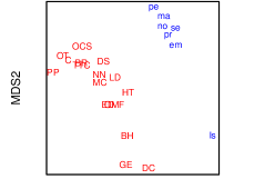
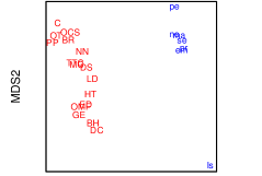
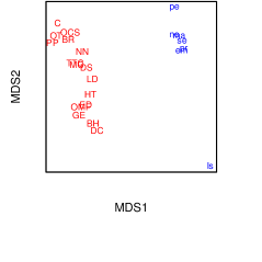
Figure 1: Cluster analysis and MDS plots based on (from top to bottom) the Euclidean distance, $d_{1}$, square root distance, $d_{\frac{1}{2}}$, and Procrustes distance, $d_{\frac{1}{2},S}$ each with $m=1000$. The plots display Austen’s novels in lower case, and Dickens’s novels in upper case.

We initially compare some choices of distance metrics on the Austen and Dickens data after constructing the graph Laplacians from the $m=1000$ most frequent words across all 23 novels. Figure 1 (left column) shows the results of a hierarchical cluster analysis using Ward’s method (Ward, 1963), based on pairwise distances between novels using metrics $d_{1}$, $d_{\frac{1}{2}}$ and $d_{\frac{1}{2},S}$. For computing the Procrustes metric we use the shapes package (Dryden, 2019) in R (R Core Team, 2020).

The dendrograms for square root and Procrustes separate the authors into two very distinct clusters, whereas for Euclidean distance Dickens’ David Copperfield and Great Expectations are clustered with Austen’s Lady Susan which is unsatisfactory. The next sub-division of the Dickens cluster using square root/Procrustes distance splits into groups of the earlier novels versus later novels, with the exception being the historical novel A Tale of Two Cities which is clustered with the earlier novels. There is not such a clear sub-division for Dickens using the Euclidean metric. In the Austen cluster for square root and Procrustes there is clearly a large distance between Lady Susan and the rest, where Lady Susan is her earliest work, a short novella published 54 years after Austen’s death.

Figure 1 (right column) shows corresponding plots of the first two multi-dimensional scaling (MDS) variables from a classical multi-dimensional scaling analysis. The square root and Procrustes MDS plots are visually identical, although they are slightly different numerically. We see that there is a clear separation in MDS space between Austen’s and Dickens’ works with a very strong separation in MDS1 using the square root and Procrustes distances, and less so for Euclidean distance. This example clearly shows differences when using the metrics, and demonstrates an advantage of using the square root Euclidean and Procrustes distances compared to the Euclidean distance here.

3 Framework for the statistical analysis of graph Laplacians

3.1 Framework

The general framework we will define in this section for the statistical analysis of graph Laplacians involves mapping, embedding and projections, shown schematically in Figure 2.

Figure 2: Schematic diagram for the general framework for the statistical analysis of graph Laplacians. The embedding map $\text{F}_{\alpha}$ and embedding space $\mathcal{M}_{m}$ are defined in Section 3.2. The identity map is denoted by $Id$. The tangent space, $T_{\nu}(\mathcal{M}_{m})$ and associated projections $\pi_{\nu}$ and $\pi_{\nu}^{-1}$ are defined in Section 3.3. The reverse power map $\text{G}_{\alpha}$ is defined in Section 3.4 and the projection $\text{P}_{\mathcal{L}}$ is defined in Section 3.5.

Distance metrics such as (5) and (6) on manifolds are referred to as intrinsic or extrinsic. An intrinsic distance is the length of a shortest geodesic path in the manifold, whereas an extrinsic distance is one induced by a Euclidean distance in an embedding of the manifold (Dryden and Mardia, 2016, p112). On $\mathcal{L}_{m}$, Euclidean distance $d_{1}$ is intrinsic, but in general $d_{\alpha}$ and $d_{\alpha,S}$ are extrinsic with respect to an embedding defined as follows.

3.2 Map and embedding

We write $\textbf{L}=\textbf{U}\boldsymbol{\Xi}\textbf{U}^{T}$ by the spectral decomposition theorem, with $\boldsymbol{\Xi}=\text{diag}(\xi_{1},\ldots,\xi_{m})$ and $\textbf{U}=(\textbf{u}_{1},\ldots,\textbf{u}_{m})$, where $\{\xi_{i}\}_{i=1,\ldots,m}$ and $\{\textbf{u}_{i}\}_{i=1,\ldots,m}$ are the eigenvalues and corresponding eigenvectors of L. We consider the following map which raises the graph Laplacian to the power $\alpha>0$:

$$\begin{split}\text{F}_{\alpha}(\textbf{L})&=\textbf{L}^{\alpha}=\textbf{U}\boldsymbol{\Xi}^{\alpha}\textbf{U}^{T}:\mathcal{L}_{m}\rightarrow Image(\mathcal{L}_{m})\subset\mathcal{M}_{m}.\\ \end{split}$$ (7)

We note that $\text{F}_{\alpha}$ is a bijective map (with inverse $\text{F}^{-1}_{\alpha}$). After applying the transformation $\text{F}_{\alpha}$ we then consider the image of the graph Laplacian space to be embedded in a manifold ${\cal M}_{m}$, where statistical analysis is carried out using extrinsic methods. We will either use the Euclidean distance $d_{E}$ (3) or the Procrustes distance $d_{S}$ (4) in the embedding manifold ${\cal M}_{m}$.

Our choice of ${\cal M}_{m}$ will depend on which metric is used. When using the Euclidean power distance we take the embedding manifold ${\cal M}_{m}$ to be the space of real symmetric $m\times m$ matrices with centred rows and columns

$$\mathcal{S}^{*}_{m}=\{\textbf{Y}=(y_{ij}):\textbf{Y}=\textbf{Y}^{T};\,\textbf{Y}{\textbf{1}_{m}}={\textbf{0}_{m}}\},$$ (8)

which has dimension $m(m-1)/2$, which is the same dimension as $\mathcal{L}_{m}$. When using the Procrustes power distance we take the embedding manifold to be the reflection size-and-shape space (Dryden, Koloydenko and Zhou, 2009; Dryden and Mardia, 2016, p67)

$$RS\Sigma^{m}_{m-1}=\{\mathbb{R}^{(m-1)^{2}}/O(m-1)\},$$ (9)

which also has dimension $m(m-1)/2$. The reflection size-and-shape space has singularities, but away from these singularity sets the space is a Riemannian manifold.

The distance metrics (5) and (6) are isometric to Euclidean distance in $\mathcal{S}^{*}_{m}$ and Procrustes distance in $RS\Sigma^{m}_{m-1}$ respectively, and can be written as

$$d_{\alpha}(\textbf{L}_{1},\textbf{L}_{2}) =\|\text{F}_{\alpha}(\textbf{L}_{1})-\text{F}_{\alpha}(\textbf{L}_{2})\|$$

$$d_{\alpha,S}(\textbf{L}_{1},\textbf{L}_{2}) =\inf_{\textbf{R}\in\mathcal{O}(m)}\|\text{F}_{\alpha}(\textbf{L}_{1})-\text{F}_{\alpha}(\textbf{L}_{2})\textbf{R}\|.$$

A suitable choice of $\alpha>0$ will be dependent on the application. Some discussion in related work on symmetric positive semi-definite matrices is relevant. Despite the swelling effect that can be present for $\alpha=1$ an advantage in this case is that we have an intrinsic distance, and the nodes are directly used in the distance calculations rather than in an embedding space. The parameter $\alpha$ behaves like a Box-Cox transformation parameter, with $\alpha=\frac{1}{2}$ a matrix square root, and $\alpha\to 0$ a matrix logarithm. Large $\alpha$ gives strong weight to the differences between the largest values in the embedding space, and small $\alpha$ gives a more even weighting between large and small values. In Pigoli et al. (2014) the authors considered metrics between covariance operators including Procrustes metrics and in the continuous case it is required that $\alpha\geq\frac{1}{2}$. In their examples $\alpha=\frac{1}{2}$ gave good results when investigating differences between languages. Dryden, Pennec and Peyrat (2010) also found $\alpha=\frac{1}{2}$ was appropriate when using Box-Cox transformation for comparing diffusion weighted images. The Procrustes distance with $\alpha=\frac{1}{2}$ between two covariance operators is the same as the Wasserstein distance between two zero mean Gaussian processes with different covariance operators (Masarotto, Panaretos and Zemel, 2019). The popularity of the Wasserstein metric as an optimal transport distance between probability distributions (e.g. Villani, 2009, Chapter 6) lends further support to using both Procrustes version and $\alpha=\frac{1}{2}$. However, ultimately it is of course up to the user whether to use Procrustes or not, and which $\alpha$ to choose. In our applications we will compare $\alpha=1$ and $\alpha=\frac{1}{2}$.

3.3 Tangent space

To perform statistical analysis we work with a tangent space at pole $\nu\in\mathcal{M}_{m}$ which we denote by $T_{\nu}(\mathcal{M}_{m})$. A projection from the tangent space $T_{\nu}(\mathcal{M}_{m})$ to $\mathcal{M}_{m}$ is written as

$$\pi_{\nu}:T_{\nu}(\mathcal{M}_{m})\to\mathcal{M}_{m}$$

with inverse projection $\pi_{\nu}^{-1}$. Standard statistical methods can be applied in the tangent space, which is a Euclidean space of dimension $m(m-1)/2$. Figure 3 shows a simple visualisation of a tangent space. The tangent space at $\nu$ is a Euclidean approximation touching the manifold $\mathcal{M}_{m}$. In non-Euclidean spaces a distance is the length of the shortest geodesic path between two points on a manifold. For specific Riemannian metrics the tangent projection could be the inverse exponential map, denoted $\exp^{-1}_{\nu}$ (Dryden and Mardia, 2016, Chapter 5), and in this case a geodesic becomes a straight line in the tangent space preserving distance to the pole.

Figure 3: A diagrammatic view of a $\pi_{\nu}^{-1}$ projection, mapping X from a manifold ${\mathcal{M}}_{m}$, here shown schematically as a sphere, onto the tangent space $T_{\nu}$.

As the graph Laplacian space has centering constraints on the rows and columns, these constraints are also preserved in our choice of map and embedding to ${\cal M}_{m}$. We can remove the centering constraints and reduce the dimensions of the matrices when projecting to a tangent space by pre and post multiplying by the $m-1\times m$ Helmert sub-matrix H and its transpose as a component of the projection. The Helmert sub matrix H, of dimension $m-1\times m$, has $j$th row defined as

$$(\underbrace{h_{j},\ldots,h_{j}}_{j\text{ times}},-jh_{j},\underbrace{0,\ldots,0}_{m-j-1\text{ times}}),\quad h_{j}=-(j(j+1))^{-\frac{1}{2}},$$

(page 49, Dryden and Mardia (2016)). Note that $\textbf{H}\textbf{H}^{T}=\mathbf{I}_{m-1}$ and $\textbf{H}^{T}\textbf{H}=\mathbf{C}_{m}$, where $\mathbf{C}_{m}=\mathbf{I}_{m}-\mathbf{1}_{m}\mathbf{1}_{m}^{T}/m$ is the $m\times m$ centering matrix, $\mathbf{I}_{m}$ is the $m\times m$ identity matrix and $\mathbf{1}_{m}$ is the $m$-vector of ones.

For the Euclidean power metric we use the inverse tangent projection $\pi_{\nu}^{-1}$ to the tangent space $T_{\nu}({\cal S}_{m}^{*})=\mathbb{R}^{\frac{m(m-1)}{2}}$ as

$$\begin{split}\pi_{\nu}^{-1}(\textbf{X})=\text{vech*}\{\textbf{H}(\textbf{X}-\nu)\textbf{H}^{T}\}\\ \pi_{\nu}(\textbf{Q})=\nu+\textbf{H}^{T}\text{vech*}^{-1}(\textbf{Q})\textbf{H}\end{split}$$ (10)

where ${\rm vech}^{*}$ is the half vectorisation of a matrix including the diagonal, similar to ${\rm vech}$, but with $\surd 2$ multiplying the elements corresponding to the off-diagonal. In this case $\mathcal{M}_{m}=\mathcal{S}_{m}^{*}$ as in (8) so has zero curvature, and analysis is unaffected by the choice of $\nu$. The use of the Helmert sub-matrix ensures that we have the correct number $m(m-1)/2$ of tangent coordinates, and is a convenient way of dealing with the centering constraints in $\mathcal{M}_{m}$.

For the Procrustes power metric we define the map $\pi_{\nu}^{-1}$ to the tangent space
$T_{\nu}(RS\Sigma^{m}_{m-1})=\mathbb{R}^{\frac{m(m-1)}{2}}$ as

$$\begin{split}\pi_{\nu}^{-1}(\textbf{X})=\text{vec}\{\textbf{H}(\textbf{X}\hat{\textbf{R}}-\nu)\textbf{H}^{T}\}\\ \pi_{\nu}(\textbf{Q})=(\nu+\textbf{H}^{T}\text{vec}^{-1}(\textbf{Q})\textbf{H})\tilde{\textbf{R}}\end{split}$$ (11)

where $\rm{vec}$ is the vectorise operator obtained from stacking the columns of a matrix, $\hat{\textbf{R}}$ is the ordinary Procrustes match of X to $\nu$ (Dryden and Mardia, 2016, chapter 7) and $\tilde{\textbf{R}}$ is the ordinary Procrustes match from $(\nu+\textbf{H}^{T}\text{vec}^{-1}(\textbf{Q})\textbf{H})$ to $\nu$. Note that the reflection size-and-shape space is a space with positive curvature (Kendall et al., 1999) and statistical analysis depends on the choice of $\nu$. A sensible choice for $\nu$ is the sample mean, as defined in Section 3.6.

3.4 Reverse power map

When transforming back from the embedding space to the graph Laplacian space we choose a practical method which involves first applying a continuous reverse power map $\textbf{G}_{\alpha}$ and then a projection $\text{P}_{\mathcal{L}}$ into graph Laplacian space:

$$\text{P}_{\mathcal{L}}\circ\textbf{G}_{\alpha}:\mathcal{M}_{m}\to\mathcal{L}_{m},$$

as illustrated in the framework in Figure 2.

We consider four choices for the reverse power map:

$$\text{G}_{\alpha}(\textbf{Q}) =\begin{cases}\quad(\textbf{Q})^{\frac{1}{\alpha}}\;\;\text{ when }\frac{1}{\alpha}\text{ is an odd integer}&:\mathcal{M}_{m}\rightarrow\mathcal{M}_{m}\\ \quad\left(\frac{\textbf{Q}+\textbf{Q}^{T}+\{(\textbf{Q}+\textbf{Q}^{T})^{T}(\textbf{Q}+\textbf{Q}^{T})\}^{\frac{1}{2}}}{4}\right)^{\frac{1}{\alpha}}&:\mathcal{M}_{m}\rightarrow\mathcal{PSD}_{m}^{*}\subseteq\mathcal{M}_{m}\\ \quad(\textbf{QQ}^{T})^{\frac{1}{2\alpha}}&:\mathcal{M}_{m}\rightarrow\mathcal{PSD}_{m}^{*}\subseteq\mathcal{M}_{m},\\ \quad(\textbf{Q}^{T}\textbf{Q})^{\frac{1}{2\alpha}}&:\mathcal{M}_{m}\rightarrow\mathcal{PSD}_{m}^{*}\subseteq\mathcal{M}_{m}.\end{cases}$$

which are suitable for different scenarios depending on whether or not we want to map to the space of centred positive semi-definite matrices $\mathcal{PSD}_{m}^{*}$ before reversing the powering of $\alpha$. In our applications we use the first choice of reverse map for Euclidean distance $d_{1}$, which is just the identity map in this case. The second expression before taking the power $\frac{1}{\alpha}$ is the closest symmetric positive semi-definite matrix to Q in terms of Frobenius distance (Higham, 1988), and we use this reverse map for $d_{\frac{1}{2}}$. The third reverse map removes the orthogonal matrix from the Procrustes match introduced from the tangent projection in (11) and was used previously by Dryden, Koloydenko and Zhou (2009). We use the fourth reverse map for $d_{\frac{1}{2},S}$ in our applications, where the orthogonal matrix from the Procrustes match is retained.

3.5 Projection

Suitable choices of projection $\text{P}_{\mathcal{L}}$ based on the Euclidean power or Procrustes power metrics are:

$$\begin{split}\text{P}_{\alpha}(\textbf{Y})&=\arg\inf_{\textbf{L}\in\mathcal{L}_{m}}d_{E}(\textbf{Y},F_{\alpha}(\textbf{L})):\mathcal{M}_{m}\rightarrow\mathcal{L}_{m}\\ \text{P}_{\alpha,S}(\textbf{Y})&=\arg\inf_{\textbf{L}\in\mathcal{L}_{m}}d_{S}(\textbf{Y},F_{\alpha}(\textbf{L})):\mathcal{M}_{m}\rightarrow\mathcal{L}_{m},\end{split}$$ (12)

where the Euclidean distance $d_{E}$ and the Procrustes distance $d_{S}$ were defined in (3) and (4), respectively.

It is desirable that optimisation involved in computing the projection is convex, since convex optimisation problems have the useful characteristic that any local minimum must be the unique global minimum (Rockafellar, 1993).

Result 1.

For $\text{P}_{1}$ the projection can be found by solving a convex optimisation problem with a unique solution, by minimising

$$\begin{split}f(\textbf{Y})&=d_{E}^{2}(\textbf{L},\textbf{Y})=\sum_{i=1}^{m}\sum_{j=1}^{m}(l_{ij}-y_{ij})^{2}\\ \text{subject to:}\quad\quad l_{ij}-l_{ji}&=0,\quad 0\leq i,j\leq m\\ \sum_{j=1}^{m}l_{ij}&=0,\quad 0\leq i\leq m\\ l_{ij}&\leq 0,\quad\quad 0\leq i,j\leq m\text{ and }i\neq j.\end{split}$$ (13)

It is immediately clear that this is a convex optimization problem since the objective function is quadratic with Hessian $2\mathbf{I}_{m(m-1)/2}$, which is strictly positive definite, and the constraints are linear. The unique global solution for the projection can be found using quadratic programming. To implement this projection $\text{P}_{1}$ we can, for example, use either the CVXR (Fu et al., 2020) or rosqp (Anderson, 2018) packages in R (R Core Team, 2020) to solve the optimisation, and rosqp is particularly fast even for $m=1000$.

Note that the choice of metric for projection does not need to be the same as the choice of metric for estimation. As the projection for the Euclidean power metric with $\alpha=1$ involves convex optimisation we will use $\text{P}_{\mathcal{L}}=\text{P}_{1}$ throughout for all our metrics. For $\alpha\neq 1$ the optimization is not in general convex.

An alternative procedure to using the reverse map followed by a projection could be to first apply a projection into the image space of graph Laplacians and then apply an inverse of the embedding map $\textbf{F}^{-1}_{\alpha}$, in a similar manner to Lin et al. (2017). This alternative approach is more difficult to work with in general for graph Laplacians, except for the Euclidean metric with $\alpha=1$ when both approaches are equivalent.

3.6 Mean estimation

There are two main types of means on a manifold: an intrinsic mean and an extrinsic mean (Dryden and Mardia, 2016, Chapter 6). We define the mean in the graph Laplacian space using extrinsic means, although the mean when the Euclidean power distance with $\alpha=1$ is used is in fact an intrinsic mean.

We define the population mean for graph Laplacians as

$$\begin{split}\mu=\text{P}_{\mathcal{L}}(\textbf{G}_{\alpha}(\eta)),\text{ where }{\eta}={\rm arg}\inf_{u\in\mathcal{M}_{m}}\textbf{E}[d^{2}(\textbf{F}_{\alpha}(\textbf{L}),u)],\end{split}$$ (14)

assuming $\eta$ exists, and $d$ is either the Euclidean or Procrustes distance in $\mathcal{M}_{m}$. We define the sample mean for a set of graph Laplacians as

$$\begin{split}\hat{\mu}=\text{P}_{\mathcal{L}}(\textbf{G}_{\alpha}(\hat{\eta})),\text{ where }\hat{\eta}={\rm arg}\inf_{u\in\mathcal{M}_{m}}\frac{1}{n}\sum_{k=1}^{n}d^{2}(\textbf{F}_{\alpha}(\textbf{L}_{k}),u),\end{split}$$ (15)

assuming $\hat{\eta}$ exists. For the Euclidean power distance we have

$${\eta} =\mathbb{E}[\text{F}_{\alpha}(\textbf{L})]$$ (16)

$$\hat{\eta} =\frac{1}{n}\sum_{k=1}^{n}\text{F}_{\alpha}(\textbf{L}_{k}),$$ (17)

where $\eta,\hat{\eta}$, and hence $\mu,\hat{\mu}$, are unique in this case. For the Euclidean power metric when $\alpha=1$, we have $\hat{\mu}=\hat{\eta}$ and the mean is a Fréchet intrinsic mean (Fréchet, 1948; Ginestet et al., 2017) in this case. An alternative discussion of the Fréchet mean is given by Kolaczyk et al. (2020) who use vectorization rather than the matrices that we use.

For the Procrustes power distance $\mu$ and $\hat{\mu}$ may be sets, and the conditions for uniqueness rely on the curvature of the space (Le, 1995). We will assume uniqueness exists throughout. In the Procrustes case we assume uniqueness up to orthogonal transformation.

Result 2.

Let $\textbf{L}_{k},\;k=1,\ldots,n$ be a random sample of i.i.d. observations from a distribution with population mean $\mu$ in (14). For the power Euclidean distance ${d}_{\alpha}$ the estimator $\hat{\mu}$, in (15), is a consistent estimator of $\mu$.

The proof of this result can be found in Appendix B. Note that a similar result holds for ${d}_{\alpha,S}$ where stronger conditions for consistency of $\hat{\eta}$ are given in Bhattacharya and Patrangenaru (2003), but the same projection argument used in the proof holds.

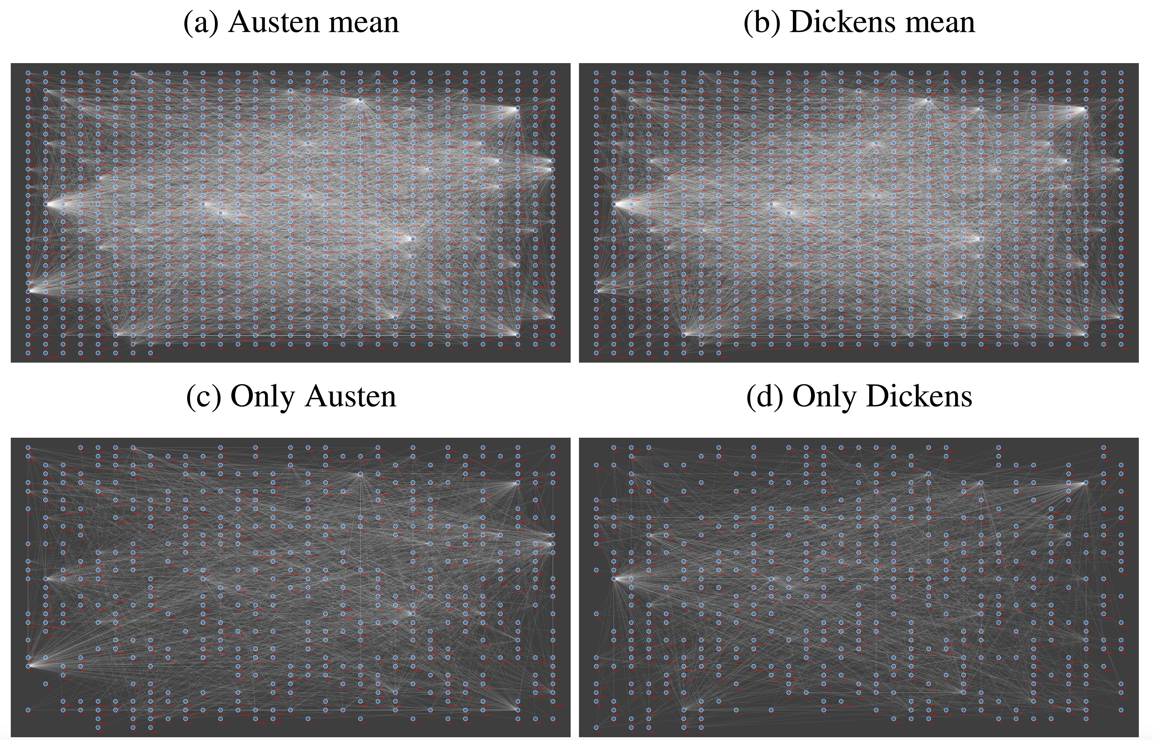
Figure 4: The means of (a) Austen’s novels and (b) Dickens’ novels using $d_{1}$ based on the top m=1000 word pairs. In (c) we see edges present in the Austen mean but not Dickens and in (d) the edges present in Dickens and not Austen means. Zoom in for more detail.

Figure 4 shows an illustration of the sample means for Austen and Dickens novels using $d_{1}$, with the 1000 words arranged in a grid and edges drawn between words which co-occur with adjacency weight at least $10^{-5}$ of the sum of the nodes. The means plots for both authors are similar, perhaps unsurprisingly as approximately half of the words in each novel are represented by the first 50 words. Figure (c) shows edges present in the Austen mean but not in the Dickens mean, and (d) the edges present in the Dickens mean but not in the Austen mean, to highlight the differences between the two networks. By zooming in, the mean plots illustrate more co-occurrences involving she, her by Austen and involving the, his, don’t by Dickens, among many others. These plots are drawn using the program Cytoscape (Shannon et al., 2003). We shall explore the differences in more detail later in Section 4.5. Alternative plots comparing the means using the Euclidean, the square root Euclidean and Procrustes metric can be found in Appendix C, and all are visually very similar.

3.7 Interpolation and extrapolation

We now consider an interpolation path,
$\textbf{L}(c)$, for $c$ being the position along the path, $0\leq c\leq 1$, between the graph Laplacians at $\textbf{L}(0)$ and $\textbf{L}(1)$. For $c<0$ and $c>1$ the path $\textbf{L}(c)$ is extrapolating from the graph Laplacians, at $\textbf{L}(0)$ and $\textbf{L}(1)$. The interpolation and extrapolation path between graph Laplacians for each metric is defined by first finding the geodesic path in the embedding space ${\cal M}_{m}$ between the embedded graph Laplacians, which is then projected to $\mathcal{L}_{m}$.

The interpolation and extrapolation path passing through $\textbf{L}_{1}=\text{P}_{\mathcal{L}}(\text{G}_{\alpha}(\nu))$ and $\textbf{L}_{2}$ is

$$\textbf{L}(c)=\text{P}_{\mathcal{L}}(\text{G}_{\alpha}(\pi_{\nu}\{c\pi_{\nu}^{-1}(\text{F}_{\alpha}(\textbf{L}_{2}))\})).$$ (18)

For the Euclidean power this simplifies to

$$\textbf{L}(c)=\text{P}_{\mathcal{L}}(\text{G}_{\alpha}(\text{F}_{\alpha}(\textbf{L}_{1})+c(\text{F}_{\alpha}(\textbf{L}_{2})-\text{F}_{\alpha}(\textbf{L}_{1})))).$$ (19)

Although these paths are geodesics in ${\cal M}_{m}$ they may not be geodesics when mapped back to the graph Laplacian space. For the Euclidean power case with $\alpha=1$ the distance $d_{1}$ is an intrinsic distance and the interpolation paths are minimal geodesics given by

$$\textbf{L}(c)=(1-c)\textbf{L}_{1}+c\textbf{L}_{2}\in\mathcal{L}_{m}\;\;\;\;0\leq c\leq 1.$$ (20)

But for $\alpha\neq 1$ and the Procrustes power metrics for any $\alpha$ the distances are extrinsic.

Figure 5 shows networks evaluated on the interpolation and extrapolation paths at $c\in\{-5,0.5,6\}$ between the mean Austen and Dickens novels when using different metrics for the 25 nodes corresponding to the most frequent words out of $m=1000$ nodes. At $c=6$ the feminine words have larger degrees and their edges have larger weights, for example her to to, of and she to to. For $c=-5$ the nodes for she and her are actually removed indicating they have degree 0, which is further evidence of the fact Austen used female words more then Dickens. The different choices of metrics lead to similar interpolation and extrapolation paths in this example, although the $d_{1}$ extrapolations are more sparse than $d_{\frac{1}{2}}$, which in turn are more sparse than $d_{\frac{1}{2},S}$.

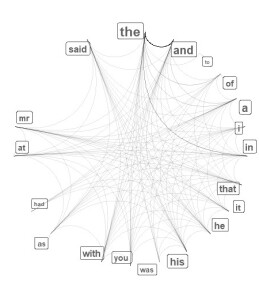
(a) $c=-5$

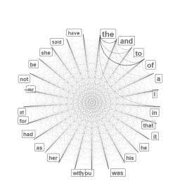
(b) $c=0.5$

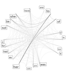
(c) $c=6$

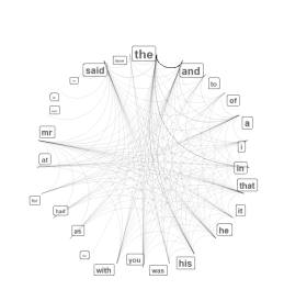
(d) $c=-5$

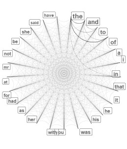
(e) $c=0.5$

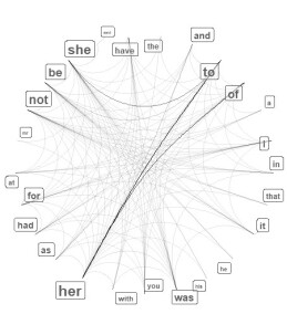
(f) $c=6$

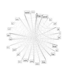
(g) $c=-5$

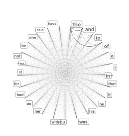
(h) $c=0.5$

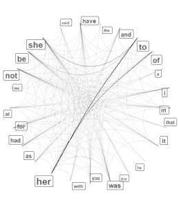
(i) $c=6$

Figure 5: Networks on the interpolation and extrapolation paths between Dickens’ and Austen’s mean novels at $c=0.5$ (interpolation) and $c=-5,c=6$ (extrapolations). Different metrics are used in each row (top to bottom) $d_{1}$, $d_{\frac{1}{2}}$ and $d_{\frac{1}{2},S}$. The top 25 words are displayed where the mean novels for the authors are estimated for each metric respectively using $m=1000$.

4 Further inference

4.1 Principal component analysis

There are several generalisations of PCA to manifold data, and the approach we define is similar to Fletcher et al. (2004), by computing PCA in a tangent space and projecting back to the manifold. Our approach differs from Fletcher et al. (2004) in that we have the extra layer of embedding the manifold and in addition we apply the reverse map and projection back to graph Laplacian space. Earlier approaches of PCA in tangent spaces in shape analysis include Kent (1994) and Cootes et al. (1994).

Let $\textbf{v}_{k}=(\pi_{\nu}^{-1}(\text{F}_{\alpha}(\textbf{L}_{k})))$, where $\nu=\hat{\eta}$ for either the Euclidean or Procrustes power metric, then $\textbf{S}=\frac{1}{n}\sum_{k=1}^{n}\textbf{v}_{k}\textbf{v}_{k}^{T}$ is an estimated covariance matrix. Suppose S is of rank $r$ with non-zero eigenvalues $\lambda_{1},\ldots,\lambda_{r}$, then the corresponding eigenvectors $\boldsymbol{\gamma}_{1},\ldots,\boldsymbol{\gamma}_{r}$ are the principal components (PCs) in the tangent space, and the PC scores are

$$s_{kj}=\boldsymbol{\gamma}_{j}^{T}\textbf{v}_{k},\quad\text{ for }k=1,\ldots,n,\quad j=1,\ldots,r.$$ (21)

The path of the $j$th PC in $\mathcal{L}_{m}$ is

$$\textbf{L}(c)=\text{P}_{\mathcal{L}}(\text{G}_{\alpha}(\,\pi_{\nu}(c\lambda_{j}^{\frac{1}{2}}\boldsymbol{\gamma}_{j})\,)),\quad c\in\mathbb{R}.$$ (22)

For the Euclidean case when $\alpha=1$ is chosen, the importance of the $i$th word in the principal component $\boldsymbol{\gamma}$ is given by

$$\frac{\pi_{\nu}(\boldsymbol{\gamma})_{ii}}{(\sum_{j=1}^{m}\pi_{\nu}(\boldsymbol{\gamma})_{jj})},\text{ for }1\leq i\leq m.$$ (23)

We now apply the methods of PCA to the pooled samples of Austen and Dickens novels, for $m=1000$. The first and second PC scores are plotted in Figure 6 for the Euclidean, square root Euclidean and Procrustes metrics. Using the Procrustes metric gave visually identical results to the square root Euclidean as we have specified the labelling of the nodes using the most common words. The extrinsic regression lines are included which we will define and explain below. The variance explained by PC 1 and PC 1 and 2 together was 49$\%$ and 70$\%$; 37$\%$ and 46$\%$; and 37$\%$ and 46$\%$ for the Euclidean, square root Euclidean and Procrustes size-and-shape respectively. A benefit of the square root Euclidean and Procrustes metric is clear here as they separate the Austen and Dickens novels with a large gap on PC1 where as David Copperfield (DC) and Persuasion (PE) are very close in PC1 for the Euclidean case. We now analyse the Euclidean PCs in more detail.

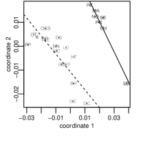
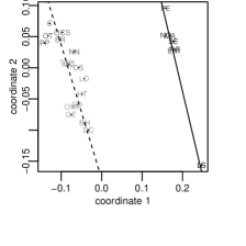
Figure 6: Plot of PC 1 and PC 2 scores for the Austen and Dickens novels, shaded in time order (black to gray, exact times can be found in Table 1) with extrinsic regression lines for Dickens novels (black) and Austen novels (dashed) using the (left) Euclidean, (middle) square root Euclidean, and (right) Procrustes size-and-shape metric.

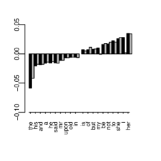
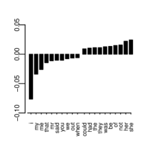
Figure 7: The importance of each word given by (23) in (left) PC 1 and (right) PC 2. The gray bars on the left represent the importance of each word in the difference of means, $\textbf{D}=\hat{\mu}^{Austen}_{E}-\hat{\mu}^{Dickens}_{E}$, given by $((\textbf{D})_{ii})/({\sum_{j=1}^{1000}({\textbf{D}})_{jj}})$, $1\leq i\leq 1000$.

Figure 7 contains plots representing the importance and sign of each word in the first and second Euclidean PC. From Figure 6 a more positive PC 1 score is indicative of an Austen novel whilst a more negative one a Dickens novel. For a positive PC1 score the nodes her and she have importance whilst for a negative score words such as his, and he have more importance, which is expected as Austen writes with more female characters. The second PC is actually similar to a fitted regression line which we describe in the next section and it is interesting to refer to the dates that the novels were written in Table 1. For Austen, the PC2 scores tend to be larger for later novels, and note that Lady Susan (LS) and Persuasion (PE) are her earliest and latest novels respectively. For Dickens the opposite is true, in that the PC2 scores tend to be smaller for later novels. Pickwick papers (PP) is Dickens’ earliest and The Mystery of Edwin Drood (ED) his latest. The second PC has feminine words like her and she as the most positive words, but more first and second person words, such as I, my and you as negative words. This is consistent with Austen increasingly using a stylistic device called free indirect speech in her later novels (Shaw, 1990). Free indirect speech has the property the third person pronouns, such as she and her are used instead of first person pronouns, such as I and my.

4.2 Regression

Here we assume the data are the pairs $\{\textbf{L}_{k},\textbf{t}_{k}\}$, for $1\leq k\leq n$ in which the $\textbf{L}_{k}\in\mathcal{L}_{m}$ are graph Laplacians to be regressed on covariate vectors $\textbf{t}_{k}=(t_{k}^{1},\ldots,t_{k}^{u})$, and consider the regression error model

$$\pi_{\nu}^{-1}(\text{F}_{\alpha}(\textbf{L}_{k}))=\text{vech}^{*}(\textbf{D}_{0}+\sum_{w=1}^{u}t_{k}^{w}\textbf{D}_{w})+\boldsymbol{\epsilon},\;\quad{\boldsymbol{\epsilon}}\sim\mathcal{N}_{m(m-1)/2}(\textbf{0},\mathbf{\Omega}).$$ (24)

In general $\mathbf{\Omega}$ has a large number of elements, so in practice it is often necessary to restrict $\mathbf{\Omega}$ to be diagonal or even isotropic, $\mathbf{\Omega}=\omega^{2}\mathbf{I}_{m(m-1)/2}$.

When using the power Euclidean metric we take $\nu=\textbf{0}$ and the parameters $\{{{\textbf{D}}}_{0},\ldots,{{\textbf{D}}}_{u}\}$ in (24) are $(m-1)\times(m-1)$ symmetric matrices, and they are estimated by solving

$$(\hat{{\textbf{D}}}_{0},\ldots,\hat{{\textbf{D}}}_{u}) =\text{arg}\min_{{{\textbf{D}}}_{0},\ldots,{{{\textbf{D}}}}_{u}}\sum_{k=1}^{n}\|\pi_{\nu}^{-1}(\text{F}_{\alpha}(\textbf{L}_{k}))-\text{vech}^{*}(\textbf{D}_{0}+\sum_{w=1}^{u}t_{k}^{w}\textbf{D}_{w})\|^{2}.$$ (25)

The fitted values are

$$\textbf{f}(\textbf{t}_{k}) =\hat{\textbf{L}}_{k}=\text{P}_{\mathcal{L}}\left(\text{G}_{\alpha}\left(\pi_{\nu}\left(\text{vech}^{*}\left(\hat{\textbf{D}}_{0}+\sum_{w=1}^{u}t_{k}^{w}\hat{\textbf{D}}_{w}\right)\right)\right)\right)\in\mathcal{L}_{m},$$ (26)

and so $\hat{\textbf{L}}_{k}$ predicts a graph Laplacian with covariates $\textbf{t}_{k}$. The optimisation in (25) is convex and the parameters of the regression line are found using the standard least squares approach in the tangent space. This optimisation reduces element-wise for $1\leq i,j\leq m$, to $m(m-1)/2$ independent optimisations. A similar model can be used for the Procrustes power metric but with $\nu=\hat{\eta}$ and with the vec operator in place of the vech* operators.

A test for the significance of covariate $t^{w}$ involves the hypotheses $H_{0}:$ $\textbf{D}_{w}=\textbf{0}$ and $H_{1}:$ $\textbf{D}_{w}\neq\textbf{0}$. By Wilks’ Theorem (Wilks, 1962), if $H_{0}$ is true then the likelihood ratio test statistic is

$$T^{\ell}=-2\log\Delta=-2\left(\sup_{\mathcal{D},\textbf{D}_{w}=\textbf{0}}\ell(\mathcal{D})-\sup_{\mathcal{D},\textbf{D}_{w}\neq\textbf{0}}\ell(\mathcal{D})\right)\sim\chi^{2}_{\frac{m(m-1)}{2}},$$ (27)

approximately when $n$ is large, where $\mathcal{D}=\{\textbf{D}_{0},\ldots,\textbf{D}_{u},\mathbf{\Omega}\}$, $\ell$ is the log-likelihood function under model (24), and $\mathbf{\Omega}$ is a diagonal matrix. Using equation (27) $H_{0}$ is rejected in favour of $H_{1}$ at the $100a\%$ significance level if $T^{\ell}$ is greater than the $(1-a)$ quantile of $\chi^{2}_{\frac{m(m-1)}{2}}$.

For the Austen and Dickens data, each novel, represented by a graph Laplacian $\textbf{L}_{k}$ is paired with the year, $t_{k}$, the novel was written. We regress the $\{\textbf{L}_{k}\}$ on the $\{t_{k}\}$ using the method above with $u=1$ for each author. To visualise the regression lines in Figure 6 we find the fitted values $\textbf{f}(t_{k})$ for many values of $t_{k}$ for the specific metrics, and project these to the PC1 and PC2 space. For each metric the regression lines seem to fit the data well, and could be used to see how writing styles have changed over time. When the test for regression was performed on the novels the p-values were extremely small ($<10^{-16}$) for both the Austen and Dickens regression lines, for the Euclidean, square root Euclidean and Procrustes size-and-shape metrics. Hence there is very strong evidence to believe that the writing style of both authors changes with time, regardless of which metric we choose.

4.3 A central limit theorem

Consider independent random samples $\textbf{A}_{k},k=1,\ldots,n$ where $F_{\alpha}(\textbf{A}_{k})$ have a distribution with mean $\mathbb{E}(F_{\alpha}(\textbf{A}))$. As the extrinsic mean is based on the arithmetic mean for the power Euclidean metrics, a central limit holds for the sample mean graph Laplacian, under the condition var$(F_{\alpha}(\textbf{A}))_{ij})$ is finite.

Result 3.

For any power Euclidean metric

$$\sqrt{n}\;{\rm vech}^{*}\left(\hat{\eta}-{\eta}\right)\xrightarrow[]{D}\mathcal{N}_{\frac{m(m-1)}{2}}\big{(}\textbf{0},\mathbf{\Sigma}\big{)},$$

as $n\to\infty$, and recall ${\rm vech}^{*}$ is the vech operator but with $\surd 2$ multiplying the terms corresponding to the off-diagonal, and $\mathbf{\Sigma}$ is a finite variance matrix.

When $\alpha=1$ this result is similar to that in Ginestet et al. (2017) although they work directly in $\mathcal{L}_{m}$ whereas we work in the embedding space. For the Procrustes power metric a similar central limit theorem result follows providing the more stringent conditions of Bhattacharya and Patrangenaru (2005) hold.

4.4 Hypothesis tests

Consider two populations $\mathcal{A}$ and $\mathcal{B}$ of $m\times m$ graph Laplacians with corresponding population means $\mu_{A}$ and $\mu_{B}$ defined in (14) . Given two independent random samples $\{\textbf{A}_{1},\textbf{A}_{2},\ldots,\textbf{A}_{n_{A}}\}$ and $\{\textbf{B}_{1},\textbf{B}_{2},\ldots,\textbf{B}_{n_{B}}\}$ respectively from $\mathcal{A}$ and $\mathcal{B}$, the goal is to test the hypotheses

$$H_{0}:\mu_{A}=\mu_{B}\text{ and }H_{1}:\mu_{A}\neq\mu_{B}.$$

We define the test statistic as $T=d(\hat{\textbf{A}},\hat{\textbf{B}})^{2}$, where $\hat{\textbf{A}}$ and $\hat{\textbf{B}}$ are defined by $\hat{\eta}$ in (15) for the sets $\mathcal{A}$ and $\mathcal{B}$ respectively and using a suitable metric. Any Euclidean or Procrustes power metric is suitable to use, we however will just consider the Euclidean $T_{E}=d_{1}(\hat{\textbf{A}}_{E},\hat{\textbf{B}}_{E})^{2}$; the square root Euclidean $T_{H}={d}_{\frac{1}{2}}(\hat{\textbf{A}}_{H},\hat{\textbf{B}}_{H})^{2}$; and the Procrustes size-and-shape $T_{S}={d}_{\frac{1}{2},S}(\hat{\textbf{A}}_{S},\hat{\textbf{B}}_{S})^{2}$, where the subscripts $\{E,H,S\}$ refer to whether the Euclidean, square root or Procrustes size-and-shape means have been used, respectively.

Using Result 3, the distribution of the test statistics for large $n$ is given as follows for the power Euclidean metric.

Result 4.

Consider independent random samples of networks of size $n_{A}$ and $n_{B}$. For the power Euclidean metric under the null hypothesis, $H_{0}$: $\mu_{A}=\mu_{B}$, as $n_{A},n_{B}\to\infty$, such that $n_{A}/n_{B}\to r\in(0,\infty)$:

$$\frac{n_{A}n_{B}}{n_{A}+n_{B}}d_{\alpha}(\hat{\textbf{A}},\hat{\textbf{B}})^{2}\;\xrightarrow[]{D}\;\sum_{i=1}^{m(m-1)/2}\delta_{i}\chi_{1}^{2},$$ (28)

in which each $\chi_{1}^{2}$ is independent and $\delta_{i}$ are the $m(m-1)/2$ non-zero eigenvalues of $\mathbf{\Sigma}=\frac{n_{B}\boldsymbol{\Sigma}_{A}+n_{A}\boldsymbol{\Sigma}_{B}}{n_{A}+n_{B}}$, where $\boldsymbol{\Sigma}_{A}$ and $\boldsymbol{\Sigma}_{B}$ are the population covariance matrices from Result 3 for the respective samples.

In practice $\mathbf{\Sigma}$ needs to be estimated, which can be very high dimensional. In our application with $m=1000$ this is a symmetric matrix with $M(M+1)/2$ parameters where $M=m(m-1)/2=499500$. One approach is to use the shrinkage estimator from Schäfer and Strimmer (2005), as employed by Ginestet et al. (2017), but this is impractical for our application with $m=1000$. If we assume a diagonal matrix $\mathbf{\Sigma}=\mathbf{\Lambda^{*}}$ then the $\delta_{i}$ correspond to the variances of individual components of the difference in means, and these can be estimated consistently from method of moments estimators. A further very simple model would be to have an isotropic covariance matrix with covariance matrix $\mathbf{\Sigma}=\sigma^{2}\textbf{I}_{m(m-1)/2}$, which requires estimation of a single variance parameter $\sigma^{2}$. Note that the likelihood ratio test for regression with test statistic $-2\log\Delta$ in Section 4.2 gives an alternative test for equality of means when the covariates are group labels, but the additional assumption of normality for the observations needs to be made in that case.

An alternative non-parametric test, which does not depend on large sample asymptotics is a random permutation test, similar to Preston and Wood (2010) as follows.

1:  Calculate the test statistics between $\mathcal{A}$ and $\mathcal{B}$, given by $T=T(\mathcal{A},\mathcal{B})$ .

2:  Generate random sets $\mathcal{A}^{*}$ and $\mathcal{B}^{*}$ of size $|\mathcal{A}|$ and $|\mathcal{B}|$ respectively, by randomly sampling without replacement from $\mathcal{A}\cup\mathcal{B}$.

3:  Compute the test statistic of sets $\mathcal{A}^{*}$ and $\mathcal{B}^{*}$, given by $T^{*}=T(\mathcal{A}^{*},\mathcal{B}^{*})$.

4:  Repeat steps 2 and 3 $r$ times, to give test statistics $T^{*}_{1},T^{*}_{2},\ldots,T^{*}_{r}$ .

5:  Order the test statistics $T^{*}(1)\leq T^{*}(2)\leq\ldots\leq T^{*}(r)$.

6:  Calculate the p-value, which is $1-\frac{j}{r}$ for the minimum $1\leq j\leq r-1$ satisfying
$T^{*}(j)<T\leq T^{*}(j+1)$, unless $T\leq T^{*}(1)$, in which case the p-value is 1 or if $T>T^{*}(r)$, in which case the p-value is 0.

Algorithm 1 Random permutation test to test the equality of means for two sets of graph Laplacians, $\mathcal{A}$ and $\mathcal{B}$, using the test statistic $T$.

A limitation of using the permutation test is it assumes exchangeability of the observations under the null hypothesis (Amaral, Dryden and Wood, 2007). This means under the null hypothesis the populations $\mathcal{A}$ and $\mathcal{B}$ are assumed identical. A test based on the bootstrap is an alternative possibility, which requires weaker assumptions about $\mathcal{A}$ and $\mathcal{B}$, see for example Amaral, Dryden and Wood (2007).

For the Austen and Dickens data have test statistics $T_{E}=0.0011$, $T_{H}=0.2759$, $T_{S}=0.0691$. We compute the p-value from the permutation test with $r=199$ permutations for each of $T_{E},T_{H},T_{S}$ and in each case all permuted values were less than the observed statistics for the data. Hence, in each case the estimated p-value is zero, indicating very strong evidence for a difference in mean graph Laplacian.

4.5 Exploring differences between authors

The result that the Austen and Dickens novels are highly significantly different is not unexpected due to the clear difference between Austen and Dickens’ novels seen in the PCA plot in Figure 6. Also, high-dimensional multivariate tests of global differences are often significant due to the nature of high-dimensional spaces, where random observations become approximately orthogonal to each other as the dimension increases (Hall, Marron and Neeman, 2005). To address this issue further we now focus on the main edge-specific differences between the Austen and Dickens networks, which is of strong practical interest.

In particular we examine the off-diagonal elements of $\hat{\mu}^{Austen}_{E}-\hat{\mu}^{Dickens}_{E}$ i.e. the differences in the mean weighted adjacency matrix, and compare them to appropriate measures of standard error of the differences using a $z$-statistic. The histograms of the off-diagonal individual graph Laplacians are heavy tailed, and a plot of sample standard deviations versus sample means show an overall average linear increase with approximate slope $\beta=0.2$, but with a large spread. We shall use this relationship in a regularised estimate of our choice of standard error.

For a particular co-occurrence pair of words we have weighted adjacency values $x_{i},i=1,\ldots,n_{A}$ and $y_{j},j=1,\ldots,n_{B}$ with sample means $\bar{x}$ and $\bar{y}$, and sample standard deviations $s_{x}$ and $s_{y}$. For our analysis here we use the Euclidean mean graph Laplacians. We estimate the variance in our sample with a weighted average of the sample variance and an estimate based on the linear relationship between the mean and standard deviation, and in particular the population pooled variance is estimated by

$$s_{p}^{2}=\frac{{n_{A}}(w_{A}s_{x}^{2}+(1-w_{A})\beta^{2}\bar{x}^{2})+{n_{B}}(w_{B}s_{y}^{2}+(1-w_{B})\beta^{2}\bar{y}^{2})}{(n_{A}+n_{B}-2)},$$

where the weights are taken as $w_{A}=n_{A}/N,w_{B}=n_{B}/N$, where we take $N=200$. Note that if all values in one of the samples are $0$ (due to no word co-occurrence pairings in any of that author’s books) then we drop that word pairing from further analysis, as we are only interested in the relative usage of the word occurrences that are actually used by both authors. A univariate $z$-statistic for comparing adjacencies is then

$$z=\frac{\bar{x}-\bar{y}}{(q+s_{p})\sqrt{\frac{1}{n_{A}}+\frac{1}{n_{B}}}},$$ (29)

where we include the regularizing offset $q>0$ to avoid highlighting very small differences in mean adjacency with very small standard errors. The value for $q$ is chosen as the median of all $s_{p}$ values under consideration.

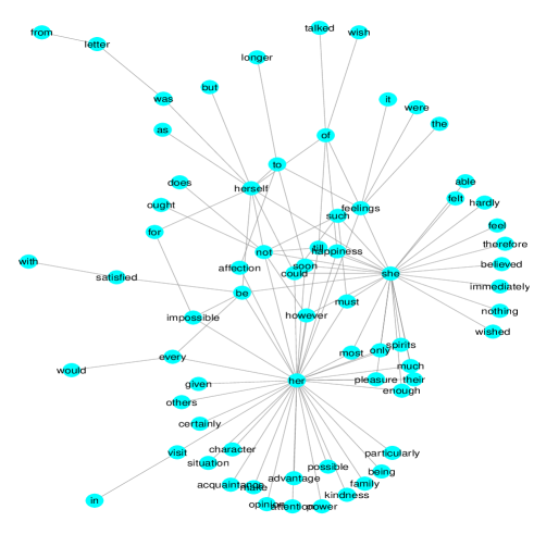
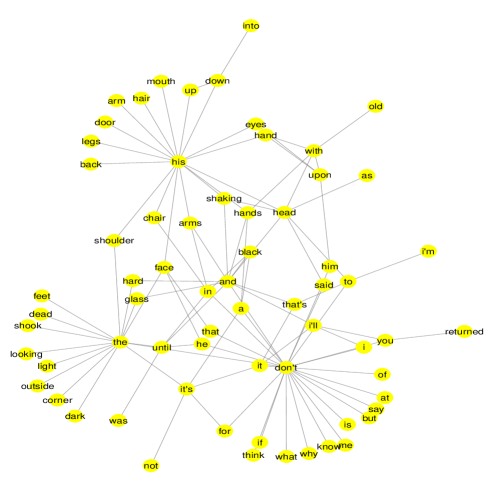
Figure 8: Networks displaying the top 100 pairs of words ranked according to the $z$-statistic in (29), with more prominent co-occurrences used by Austen (top) and the more prominent co-occurrences used by Dickens (below).

Exploratory graphical displays are given in Figure 8 as networks where an edge is drawn between two words if they appear in the top 100 pairs of words ranked according to the $z$-statistic in (29). The plots show the more prominent co-occurrences used by Austen and the more prominent co-occurrences used by Dickens, respectively. The displays illuminate striking differences between the novelists. For Austen there are very common pairings of words with her, she, herself, which form important hubs in this network. Austen also pairs these hubs with more emotional words feelings, felt, feel, kindness, happiness, affection, pleasure and stronger words power, attention, must, certainly, advantage and opinion. Also we see more use of letter in Austen, which is a literary device often used by the author. For Dickens there are more common uses of abbreviations, especially don’t which is an important hub, and also it’s, i’ll and that’s. In contrast the Austen network highlights not. Dickens also more prominently pairs body parts arm, arms, eyes, feet, hair, hand, hands, head, mouth, face, shoulder, legs in combination with the strong hubs his and the. These hubs are also paired with other objects, such as door, chair, glass. Finally, Dickens has the more prominent use of pairs with a sombre word, such as dark, black and dead, which might have been expected.

5 Conclusion

We have developed a general framework for the statistical analysis of graph Laplacians and considered in particular the power Euclidean, $d_{\alpha}$, and Procrustes size-and-shape, $d_{\alpha,S}$, metrics. The framework is extrinsic except when $d_{1}$ is used. Other metrics fit in our extrinsic framework and could be considered. One example is the log metric used in Bakker, Halappanavar and Sathanur (2018) which uses the embedding $\text{F}_{\log}(\textbf{L})=\sum_{i=1}^{l}\log{(\xi_{i})}\textbf{u}_{i}\textbf{u}_{i}^{T}$, and $\text{F}_{\log}(\textbf{L})=\lim_{\alpha\rightarrow 0}\frac{1}{\alpha}(\text{F}_{\alpha}(\textbf{L})-\text{F}_{0}(\textbf{L})$) where we define $0^{0}=0$ in $\text{F}_{0}$ and $l$ is the rank of L. The metric is then $d_{\log}(\textbf{L}_{1},\textbf{L}_{2})=\|\text{F}_{\log}(\textbf{L}_{1})-\text{F}_{\log}(\textbf{L}_{2})\|$. The log embedding is a natural embedding to consider in more detail in further work and to compare the properties of the log embedding methods with using $\textbf{F}_{\alpha}$. The log embedding been used successfully in many applications, for example for symmetric positive definite matrices extracted from diffusion tensor imaging (DTI) in Bhattacharya and Lin (2017). An extrinsic regression model similar to the ours but using kernel regression has been developed for manifolds by Lin et al. (2017), and in future work it would be worth investigating if their results extend to the $\textbf{F}_{\alpha}$ embedding.

Another metric to consider is the element-wise metric of the form
$d_{\rho}^{*}(\textbf{L}_{1},\textbf{L}_{2})=(\sum_{i}\sum_{j}|(\textbf{L}_{1})_{ij}-(\textbf{L}_{2})_{ij}|^{\rho})^{\frac{1}{\rho}}$. Of particular interest would be comparing $\rho=2$, which is the Frobenius/Euclidean norm $d_{1}$, with $\rho=1$ which can be similar to the square root norm (and is identical for diagonal matrices).

One practical issue is the estimation of covariance matrices in models for graph Laplacians. In general for $m$ by $m$ graph Laplacians the covariance matrix $\mathbf{\Omega}$ has a very large number $\frac{m(m-1)(m^{2}-m+2)}{8}$ of parameters in the regression model (24). A very large number $n$ of networks would be needed for estimating the most general form of the model, and so in practice we assume that the covariance matrix is diagonal. Extending to non-diagonal parameterised covariance structures could also be sometimes feasible, e.g. autoregressive models or covariance structure based on the spatial location of the nodes if that makes sense in particular applications.

In our application we have ordered the 1000 word lists, and we used the ordering of the most common words from the combined set of novels of both authors. Although the ordering of most common words is different in each novel, there is consistency in the broad ordering of common words. It does make sense in our application to keep a common ordering, and the effect of using the Procrustes distance versus the power metric is not so large, as we have seen. However, in other applications where there is a less obvious correspondence between nodes, the Procrustes distance could be very different.

Our methodology gives appropriate results for comparing co-occurrence networks for Jane Austen and Charles Dickens novels, but the methodology is widely applicable, for example to neuroimaging networks and social networks, and such applications will be explored in further work.

Appendix A Most common words

	Rank in	Rank in	Rank in
Word	all	Dickens	Austen
	novels	novels	novels
the	1	1	1
and	2	2	3
to	3	3	2
of	4	4	4
a	5	5	5
i	6	6	7
in	7	7	8
that	8	8	13
it	9	11	10
he	10	10	16
his	11	9	20
was	12	13	9
you	13	12	15
with	14	14	21
her	15	16	6
as	16	15	18
had	17	17	17
for	18	20	19
at	19	21	25
mr	20	18	38
not	21	26	12
be	22	28	14
she	23	31	11
said	24	19	58
have	25	25	23

Table 2: The most common 25 words in the Austen and Dickens novels

Appendix B Proof for result 2

Let $\{\hat{\theta}_{n}\}$ be a sequence of estimates from a sample set of graph Laplacians
$\{\textbf{L}_{1},\ldots,\textbf{L}_{n}\}$ for a population parameter $\theta$. For $\hat{\theta}_{n}$ to be consistent it converges in probability to $\theta$ as $n\to\infty$, i.e. for any $\epsilon>0,\delta>0$ there exists a number $N$ such that for all $n\geq N$ we have $P(|\hat{\theta}_{n}-\theta|>\epsilon)<\delta$.

When using the power metric $d_{\alpha}$ we have the embedding space ${\mathcal{M}}_{m}$ as a Euclidean space. Hence, we know that $\hat{\eta}\in{\mathcal{M}}_{m}$ is a consistent estimator of $\eta\in\mathcal{M}_{m}$, as it converges in probability to $\eta$ from the law of large numbers, where $\hat{\eta},\eta$ are defined in (16),(17). So by the continuous mapping theorem $\textbf{G}_{\alpha}(\hat{\eta})$ converges in probability to $\textbf{G}_{\alpha}(\eta)$ as $n\to\infty$.

(a) Case 1

(b) Case 2

Figure 9: 2D representations of the possibly high dimensional faces of $\mathcal{L}_{m}$ illustrating convergence of means.

We now need to show the convergence in probability holds when we project to $\mathcal{L}_{m}$. Recall that $\mathcal{L}_{m}\subset\mathcal{M}_{m}$ and both spaces have dimension $\frac{m(m-1)}{2}$. Ginestet et al. (2017) showed that $\mathcal{L}_{m}$ is a closed compact convex subset of an affine space, i.e. each face of $\mathcal{L}_{m}$ is isometric to a subset of $[0,\infty)^{k}\times\mathbb{R}^{d-k}$ for some $k>0$. Hence the interior of each face of $\mathcal{L}_{m}$ has zero curvature, and we denote the boundary of $\mathcal{L}_{m}$ as $\mathcal{B}(\mathcal{L}_{m})$. Let $\beta=|\textbf{G}_{\alpha}(\hat{\eta})-\textbf{G}_{\alpha}(\eta)|$ and $\zeta=|\hat{\mu}-\mu|$.

There are three cases to consider:

• Case 1: ${\mu}$ is in $\mathcal{B}(\mathcal{L}_{m})$ but not on a corner. In this case the estimator behaves as in Figure 9(a). The estimator $\textbf{G}_{\alpha}(\hat{\eta})$ is orthogonally projected to $\hat{\mu}$, hence due to Pythagoras’ theorem it is clear $\zeta\leq\beta$.

• Case 2: $\mu$ is on a corner of $\mathcal{B}(\mathcal{L}_{m})$. In this case the estimator behaves as in Figure 9(b). Clearly $\frac{\pi}{2}\leq\vartheta\leq\pi$ as $\mathcal{L}_{m}$ is convex (Ginestet et al., 2017). We consider a point $q$ along the line between $\textbf{G}_{\alpha}(\hat{\eta})$ and $\textbf{G}_{\alpha}(\eta)$ such that the angle between $\hat{\mu}$, $\mu$ and $q$ is $\frac{\pi}{2}$. Note $\zeta\leq|\textbf{G}_{\alpha}(\hat{\eta})-q|$ following identical arguments as in case 1, and clearly $|\textbf{G}_{\alpha}(\hat{\eta})-q|\leq\beta$. Hence $\zeta\leq\beta$.

• Case 3: ${\mu}$ is in the interior of $\mathcal{L}_{m}$, and so $\textbf{G}_{\alpha}(\eta)=\mu$ and by Pythagoras’ theorem $\zeta\leq\beta$.

From the consistency of $\textbf{G}_{\alpha}(\hat{\eta})$ for any $\epsilon>0,\delta>0$ there exists an $N$ such that for $n\geq N$ then $P(|\textbf{G}_{\alpha}(\hat{\eta})-\textbf{G}_{\alpha}(\eta)|>\epsilon)<\delta$. So, in all three cases we deduce that

$$P(|\hat{\mu}-\mu|>\epsilon)=P(\zeta>\epsilon)\leq P(\beta>\epsilon)=P(|\textbf{G}_{\alpha}(\hat{\eta})-\textbf{G}_{\alpha}(\eta)|>\epsilon)<\delta$$

and so $\hat{\mu}$ converges in probability to $\mu$, i.e. $\hat{\mu}$ is a consistent estimator for $\mu$.

Appendix C Means for Austen’s and Dickens’ novels

Figure 10: The means of (left) Austen’s novels and (right) Dickens’ novels using $d_{1}$ (first row), $d_{\frac{1}{2}}$ (middle row) and $d_{\frac{1}{2},S}$ (bottom row) based on the top m=1000 word pairs. Zoom in for more detail.

References

- Amaral, Dryden and Wood (2007) {barticle}[author] \bauthor\bsnmAmaral, \bfnmG. J. A\binitsG. J. A., \bauthor\bsnmDryden, \bfnmI. L\binitsI. L. and \bauthor\bsnmWood, \bfnmAndrew T. A\binitsA. T. A. (\byear2007). \btitlePivotal Bootstrap Methods for k-Sample Problems in Directional Statistics and Shape Analysis. \bjournalJournal of the American Statistical Association \bvolume102 \bpages695-707. \bdoi10.1198/016214506000001400 \endbibitem
- Anderson (2018) {bmanual}[author] \bauthor\bsnmAnderson, \bfnmEric\binitsE. (\byear2018). \btitlerosqp: Quadratic Programming Solver using the OSQP Library \bnoteR package version 0.1.0. \endbibitem
- Bakker, Halappanavar and Sathanur (2018) {barticle}[author] \bauthor\bsnmBakker, \bfnmCraig\binitsC., \bauthor\bsnmHalappanavar, \bfnmMahantesh\binitsM. and \bauthor\bsnmSathanur, \bfnmArun Visweswara\binitsA. V. (\byear2018). \btitleDynamic graphs, community detection, and Riemannian geometry. \bjournalApplied Network Science \bvolume3 \bpages3. \endbibitem
- Bhattacharya and Lin (2017) {barticle}[author] \bauthor\bsnmBhattacharya, \bfnmRabi\binitsR. and \bauthor\bsnmLin, \bfnmLizhen\binitsL. (\byear2017). \btitleOmnibus CLTs for Fréchet means and nonparametric inference on non-Euclidean spaces. \bjournalProceedings of the American Mathematical Society \bvolume145 \bpages413–428. \endbibitem
- Bhattacharya and Patrangenaru (2003) {barticle}[author] \bauthor\bsnmBhattacharya, \bfnmRabi\binitsR. and \bauthor\bsnmPatrangenaru, \bfnmVic\binitsV. (\byear2003). \btitleLarge sample theory of intrinsic and extrinsic sample means on manifolds. \bjournalAnn. Statist. \bvolume31 \bpages1–29. \bdoi10.1214/aos/1046294456 \endbibitem
- Bhattacharya and Patrangenaru (2005) {barticle}[author] \bauthor\bsnmBhattacharya, \bfnmRabi\binitsR. and \bauthor\bsnmPatrangenaru, \bfnmVic\binitsV. (\byear2005). \btitleLarge sample theory of intrinsic and extrinsic sample means on manifolds—II. \bjournalAnn. Statist. \bvolume33 \bpages1225–1259. \bdoi10.1214/009053605000000093 \endbibitem
- Cootes et al. (1994) {bincollection}[author] \bauthor\bsnmCootes, \bfnmT. F.\binitsT. F., \bauthor\bsnmTaylor, \bfnmC. J.\binitsC. J., \bauthor\bsnmCooper, \bfnmD. H.\binitsD. H. and \bauthor\bsnmGraham, \bfnmJ.\binitsJ. (\byear1994). \btitleImage search using flexible shape models generated from sets of examples. In \bbooktitleStatistics and Images: Vol. 2 (\beditor\bfnmK. V.\binitsK. V. \bsnmMardia, ed.) \bpages111-139. \bpublisherCarfax, \baddressOxford. \endbibitem
- De Klerk (2006) {bbook}[author] \bauthor\bsnmDe Klerk, \bfnmEtienne\binitsE. (\byear2006). \btitleAspects of semidefinite programming: interior point algorithms and selected applications \bvolume65. \bpublisherSpringer Science & Business Media. \endbibitem
- Dryden (2019) {bmanual}[author] \bauthor\bsnmDryden, \bfnmI. L.\binitsI. L. (\byear2019). \btitleshapes package \bpublisherR Foundation for Statistical Computing, \baddressVienna, Austria \bnoteContributed package, Version 1.2.5. \endbibitem
- Dryden, Koloydenko and Zhou (2009) {barticle}[author] \bauthor\bsnmDryden, \bfnmIan L.\binitsI. L., \bauthor\bsnmKoloydenko, \bfnmAlexey\binitsA. and \bauthor\bsnmZhou, \bfnmDiwei\binitsD. (\byear2009). \btitleNon-Euclidean Statistics for Covariance Matrices, with Applications to Diffusion Tensor Imaging. \bjournalThe Annals of Applied Statistics \bvolume3 \bpages1102-1123. \endbibitem
- Dryden and Mardia (2016) {bbook}[author] \bauthor\bsnmDryden, \bfnmIan L.\binitsI. L. and \bauthor\bsnmMardia, \bfnmKanti V.\binitsK. V. (\byear2016). \btitleStatistical shape analysis with applications in R, \beditionsecond ed. \bseriesWiley Series in Probability and Statistics. \bpublisherJohn Wiley & Sons, Ltd., Chichester. \bdoi10.1002/9781119072492 \bmrnumber3559734 \endbibitem
- Dryden, Pennec and Peyrat (2010) {barticle}[author] \bauthor\bsnmDryden, \bfnmIan L.\binitsI. L., \bauthor\bsnmPennec, \bfnmXavier\binitsX. and \bauthor\bsnmPeyrat, \bfnmJean-Marc\binitsJ.-M. (\byear2010). \btitlePower Euclidean metrics for covariance matrices with application to diffusion tensor imaging. \bjournalarXiv e-prints \bpagesarXiv:1009.3045. \endbibitem
- Evert (2008) {barticle}[author] \bauthor\bsnmEvert, \bfnmStefan\binitsS. (\byear2008). \btitleCorpora and collocations. \bjournalCorpus linguistics. An international handbook \bvolume2 \bpages1212–1248. \endbibitem
- Fletcher et al. (2004) {barticle}[author] \bauthor\bsnmFletcher, \bfnmP Thomas\binitsP. T., \bauthor\bsnmLu, \bfnmConglin\binitsC., \bauthor\bsnmPizer, \bfnmStephen M\binitsS. M. and \bauthor\bsnmJoshi, \bfnmSarang\binitsS. (\byear2004). \btitlePrincipal geodesic analysis for the study of nonlinear statistics of shape. \bjournalIEEE transactions on medical imaging \bvolume23 \bpages995–1005. \endbibitem
- Fréchet (1948) {barticle}[author] \bauthor\bsnmFréchet, \bfnmMaurice\binitsM. (\byear1948). \btitleLes éléments aléatoires de nature quelconque dans un espace distancié. \bjournalAnnales de l’institut Henri Poincaré \bvolume10 \bpages215-310. \endbibitem
- Fu et al. (2020) {bmanual}[author] \bauthor\bsnmFu, \bfnmAnqi\binitsA., \bauthor\bsnmNarasimhan, \bfnmBalasubramanian\binitsB., \bauthor\bsnmKang, \bfnmDavid W\binitsD. W., \bauthor\bsnmDiamond, \bfnmSteven\binitsS. and \bauthor\bsnmMiller, \bfnmJohn\binitsJ. (\byear2020). \btitleCVXR: Disciplined Convex Optimization \bnoteR package version 1.0-1. \endbibitem
- Ginestet et al. (2017) {barticle}[author] \bauthor\bsnmGinestet, \bfnmCedric E\binitsC. E., \bauthor\bsnmLi, \bfnmJun\binitsJ., \bauthor\bsnmBalachandran, \bfnmPrakash\binitsP., \bauthor\bsnmRosenberg, \bfnmSteven\binitsS., \bauthor\bsnmKolaczyk, \bfnmEric D\binitsE. D. \betalet al. (\byear2017). \btitleHypothesis testing for network data in functional neuroimaging. \bjournalThe Annals of Applied Statistics \bvolume11 \bpages725–750. \endbibitem
- Hall, Marron and Neeman (2005) {barticle}[author] \bauthor\bsnmHall, \bfnmPeter\binitsP., \bauthor\bsnmMarron, \bfnmJ. S.\binitsJ. S. and \bauthor\bsnmNeeman, \bfnmAmnon\binitsA. (\byear2005). \btitleGeometric representation of high dimension, low sample size data. \bjournalJ. R. Stat. Soc. Ser. B Stat. Methodol. \bvolume67 \bpages427–444. \bmrnumberMR2155347 \endbibitem
- Higham (1988) {barticle}[author] \bauthor\bsnmHigham, \bfnmNicholas J\binitsN. J. (\byear1988). \btitleComputing a nearest symmetric positive semidefinite matrix. \bjournalLinear algebra and its applications \bvolume103 \bpages103–118. \endbibitem
- Charles Dickens Info (2020) {bmisc}[author] \bauthor\bsnmCharles Dickens Info (\byear2020). \btitleCharles Dickens Timeline. \bnotehttps://www.charlesdickensinfo.com/life/timeline/, Last accessed on 2020-08-17. \endbibitem
- Kendall et al. (1999) {bbook}[author] \bauthor\bsnmKendall, \bfnmD. G.\binitsD. G., \bauthor\bsnmBarden, \bfnmD.\binitsD., \bauthor\bsnmCarne, \bfnmT. K.\binitsT. K. and \bauthor\bsnmLe, \bfnmH.\binitsH. (\byear1999). \btitleShape and Shape Theory. \bpublisherWiley, \baddressChichester. \endbibitem
- Kent (1994) {barticle}[author] \bauthor\bsnmKent, \bfnmJohn T\binitsJ. T. (\byear1994). \btitleThe complex Bingham distribution and shape analysis. \bjournalJournal of the Royal Statistical Society. Series B (Methodological) \bpages285–299. \endbibitem
- Kolaczyk (2009) {bbook}[author] \bauthor\bsnmKolaczyk, \bfnmEric D\binitsE. D. (\byear2009). \btitleStatistical analysis of network data: methods and models. \bpublisherSpringer Science & Business Media. \endbibitem
- Kolaczyk et al. (2020) {barticle}[author] \bauthor\bsnmKolaczyk, \bfnmEric D.\binitsE. D., \bauthor\bsnmLin, \bfnmLizhen\binitsL., \bauthor\bsnmRosenberg, \bfnmSteven\binitsS., \bauthor\bsnmWalters, \bfnmJackson\binitsJ. and \bauthor\bsnmXu, \bfnmJie\binitsJ. (\byear2020). \btitleAverages of unlabeled networks: Geometric characterization and asymptotic behavior. \bjournalAnn. Statist. \bvolume48 \bpages514–538. \bdoi10.1214/19-AOS1820 \endbibitem
- Le (1995) {barticle}[author] \bauthor\bsnmLe, \bfnmHuiling\binitsH. (\byear1995). \btitleMean Size-and-Shapes and Mean Shapes: A Geometric Point of View. \bjournalAdvances in Applied Probability \bvolume27 \bpages44–55. \endbibitem
- Lin et al. (2017) {barticle}[author] \bauthor\bsnmLin, \bfnmLizhen\binitsL., \bauthor\bsnmSt. Thomas, \bfnmBrian\binitsB., \bauthor\bsnmZhu, \bfnmHongtu\binitsH. and \bauthor\bsnmDunson, \bfnmDavid B\binitsD. B. (\byear2017). \btitleExtrinsic local regression on manifold-valued data. \bjournalJournal of the American Statistical Association \bvolume112 \bpages1261–1273. \endbibitem
- Mahlberg et al. (2016) {barticle}[author] \bauthor\bsnmMahlberg, \bfnmMichaela\binitsM., \bauthor\bsnmStockwell, \bfnmPeter\binitsP., \bauthor\bparticlede \bsnmJoode, \bfnmJohan\binitsJ., \bauthor\bsnmSmith, \bfnmCatherine\binitsC. and \bauthor\bsnmO’Donnell, \bfnmMatthew Brook\binitsM. B. (\byear2016). \btitleCLiC Dickens: novel uses of concordances for the integration of corpus stylistics and cognitive poetics. \bjournalCorpora \bvolume11 \bpages433-463. \bdoi10.3366/cor.2016.0102 \endbibitem
- Masarotto, Panaretos and Zemel (2019) {barticle}[author] \bauthor\bsnmMasarotto, \bfnmV.\binitsV., \bauthor\bsnmPanaretos, \bfnmV. M.\binitsV. M. and \bauthor\bsnmZemel, \bfnmY.\binitsY. (\byear2019). \btitleProcrustes Metrics on Covariance Operators and Optimal Transportation of Gaussian Processes. \bjournalSankhya A \bvolume81 \bpages172–213. \endbibitem
- The Jane Austen Society of North America (2020) {bmisc}[author] \bauthor\bsnmThe Jane Austen Society of North America (\byear2020). \btitleJane Austen’s Works. \bnotehttp://jasna.org/austen/works/, Last accessed on 2020-08-17. \endbibitem
- Phillips (1983) {bbook}[author] \bauthor\bsnmPhillips, \bfnmM. K.\binitsM. K. (\byear1983). \btitleLexical Macrostructure in Science Text. \bpublisherUniversity of Birmingham. \endbibitem
- Pigoli et al. (2014) {barticle}[author] \bauthor\bsnmPigoli, \bfnmDavide\binitsD., \bauthor\bsnmAston, \bfnmJohn A. D.\binitsJ. A. D., \bauthor\bsnmDryden, \bfnmIan L.\binitsI. L. and \bauthor\bsnmSecchi, \bfnmPiercesare\binitsP. (\byear2014). \btitleDistances and inference for covariance operators. \bjournalBiometrika \bvolume101 \bpages409–422. \bdoi10.1093/biomet/asu008 \bmrnumber3215356 \endbibitem
- Preston and Wood (2010) {barticle}[author] \bauthor\bsnmPreston, \bfnmS. P.\binitsS. P. and \bauthor\bsnmWood, \bfnmA. T. A.\binitsA. T. A. (\byear2010). \btitleTwo-Sample Bootstrap Hypothesis Tests for Three-Dimensional Labelled Landmark Data. \bjournalScandinavian Journal of Statistics \bvolume37 \bpages568–587. \endbibitem
- Rockafellar (1993) {barticle}[author] \bauthor\bsnmRockafellar, \bfnmR Tyrrell\binitsR. T. (\byear1993). \btitleLagrange multipliers and optimality. \bjournalSIAM review \bvolume35 \bpages183–238. \endbibitem
- Schäfer and Strimmer (2005) {barticle}[author] \bauthor\bsnmSchäfer, \bfnmJuliane\binitsJ. and \bauthor\bsnmStrimmer, \bfnmKorbinian\binitsK. (\byear2005). \btitleA shrinkage approach to large-scale covariance matrix estimation and implications for functional genomics. \bjournalStatistical applications in genetics and molecular biology \bvolume4 \bpagesArticle32. \endbibitem
- Shannon et al. (2003) {barticle}[author] \bauthor\bsnmShannon, \bfnmP.\binitsP., \bauthor\bsnmMarkiel, \bfnmA.\binitsA., \bauthor\bsnmOzier, \bfnmO.\binitsO., \bauthor\bsnmBaliga, \bfnmN. S.\binitsN. S., \bauthor\bsnmWang, \bfnmJ. T.\binitsJ. T., \bauthor\bsnmRamage, \bfnmD.\binitsD., \bauthor\bsnmAmin, \bfnmN.\binitsN., \bauthor\bsnmSchwikowski, \bfnmB.\binitsB. and \bauthor\bsnmIdeker, \bfnmT.\binitsT. (\byear2003). \btitleCytoscape: a software environment for integrated models of biomolecular interaction networks. \bjournalGenome Research \bvolume13 \bpages2498–2504. \endbibitem
- Shaw (1990) {barticle}[author] \bauthor\bsnmShaw, \bfnmNarelle\binitsN. (\byear1990). \btitleFree Indirect Speech and Jane Austen’s 1816 Revision of Northanger Abbey. \bjournalStudies in English Literature, 1500-1900 \bvolume30 \bpages591–601. \endbibitem
- R Core Team (2020) {bmanual}[author] \bauthor\bsnmR Core Team (\byear2020). \btitleR: A Language and Environment for Statistical Computing \bpublisherR Foundation for Statistical Computing, \baddressVienna, Austria. \endbibitem
- Villani (2009) {bbook}[author] \bauthor\bsnmVillani, \bfnmCédric\binitsC. (\byear2009). \btitleOptimal Transport: Old and New. \bpublisherSpringer, \baddressBerlin. \endbibitem
- Ward (1963) {barticle}[author] \bauthor\bsnmWard, \bfnmJoe H.\binitsJ. H. \bsuffixJr. (\byear1963). \btitleHierarchical grouping to optimize an objective function. \bjournalJ. Amer. Statist. Assoc. \bvolume58 \bpages236–244. \bmrnumberMR0148188 (26 ##5696) \endbibitem
- Wilks (1962) {bbook}[author] \bauthor\bsnmWilks, \bfnmS. S.\binitsS. S. (\byear1962). \btitleMathematical Statistics. \bpublisherWiley, \baddressNew York. \endbibitem