$\mathcal{L}_{2}$ Observers for Nonlinear Systems with Unbounded Unknown Inputs

$\mathcal{L}_{2}$ Observers for a Class of Nonlinear Systems with Unknown Inputs

[Full version of paper presented in European Control Conference, 2019]

Abstract

We consider the problem of estimating the state and unknown input for a large class of nonlinear systems subject to unknown exogenous inputs. The exogenous inputs themselves are modeled as being generated by a nonlinear system subject to unknown inputs. The nonlinearities considered in this work are characterized by multiplier matrices that include many commonly encountered nonlinearities. We obtain a linear matrix inequality (LMI), that, if feasible, provides the gains for an observer which results in certified $\mathcal{L}_{2}$ performance of the error dynamics associated with the observer. We also present conditions which guarantee that the $\mathcal{L}_{2}$ norm of the error can be made arbitrarily small and investigate conditions for feasibility of the proposed LMIs.

1 Introduction

Exogenous unknown inputs acting on a dynamical system (plant) can result in compromised safety and degraded performance. One way to protect a system against such unknown attacks is by employing unknown input observers (UIOs), as reported in [1] and [2]. Common estimation frameworks for systems in which one assumes stochastic models for the unknown exogeneous input include Kalman filtering [3] and minimum variance filters [4]. For unknown exogeneous inputs where underlying statistics are not available and cannot be guessed, methods that have proven effective include: adaptive estimation [5], sliding mode observers [6, 7], and observers that minimize the system’s input-output gain such as $\mathcal{H}_{\infty}$ observers [8, 9, 10, 11]. Recent work has produced many effective methods for generating unknown input observers for nonlinear systems; see for example [12, 13, 14, 15, 16, 17, 18, 19].

A common underlying assumption in many of the cited works is that the unknown exogeneous input is bounded. One way of relaxing that assumption is by using an extended state observer, that is, by appending the exogenous input to the system state. Exogenous input estimation via an extended state observer has been successful in various practical systems, including robotic systems [20], electric drive systems [21], power electronics [22], and avionics [23]. These exogenous inputs could be completely unknown, or partially unknown. In this paper, we refer to partially unknown inputs as exogenous inputs that have been generated by a completely unknown input acting on in [24, 25]. Although prior investigations into extended state observer design for estimation with unknown exogenous inputs has yielded useful results [26, 27, 28], the authors assume that the inputs are bounded, and tackle linear systems or linearized versions of nonlinear systems; the sparsity of results on observers for nonlinear systems with unknown deterministic exogenous inputs motivates the present paper.

In this paper, we propose extended state observers to estimate the state and the unknown exogenous input for nonlinear systems whose nonlinearities satisfy so-called incremental quadratic constraints [29, 30]. Such nonlinearities encompass a wide range of nonlinearities including globally Lipschitz, one-sided Lipschitz, monotonic and other commonly occurring nonlinearities. Also, the exogenous input can be unbounded. Observer design is based on a linear matrix inequality which we demonstrate is satisfied by a large class of commonly encountered nonlinear systems. The observers guarantee that the input-output system from exogenous input to observer error is $\mathcal{L}_{2}$-stable with a specific gain; for linear systems this gain is an upper bound on the $\mathcal{H}_{\infty}$ norm of the system. We also present conditions which guarantee that an arbitrarily small $\mathcal{L}_{2}$ gain can be achieved.

2 Problem statement

2.1 Systems under consideration

Consider a nonlinear time-varying system (the plant) described by

$$\dot{x}\; =\;Ax\; + \;B_{f}f_{1}(t,y,q_{1})\; + \;g_{x}(t,y)\; + \;Bw,$$ (1a)

$$q_{1}\; =\;C_{q_{1}}x\; + \;D_{q_{1}f}f_{1}(t,y,q_{1})\; + \;g_{q_{1}}(t,y)\; + \;D_{q_{1}}w,$$ (1b)

$$y\; =\;Cx\; + \;D_{f}f_{1}(t,y,q_{1})\; + \;g_{y}(t,y)\; + \;Dw.$$ (1c)

Here, $t\in\mathbb{R}$ is the time variable, $x(t)\in\mathbb{R}^{n_{x}}$ is the state, $y(t)\in\mathbb{R}^{n_{y}}$ is the measured output and $w(t)\in\mathbb{R}^{n_{w}}$ models the disturbance input and the measurement noise combined into one term; we refer to it as the exogenous input; this is unknown at every $t$. The vector $f_{1}(t,y,q_{1})\in\mathbb{R}^{n_{f_{1}}}$ models nonlinearities of known structure, but because this term depends on the state $x$ (through $q_{1}$), it cannot be instantaneously determined from measurements. The vector $q_{1}\in\mathbb{R}^{n_{q_{1}}}$ is a state-dependent argument of the nonlinearity $f_{1}$. The vectors $g_{x}(t,y)\in\mathbb{R}^{n_{x}}$, $g_{q}(t,y)\in\mathbb{R}^{n_{q}}$ and $g_{y}(t,y)\in\mathbb{R}^{n_{y}}$ represent nonlinearities which can be calculated instantaneously from measurements. An example is $g_{x}(t,y)=u(t)$ where $u(t)$ is a control input. All the matrices are constant and of appropriate dimensions.

We consider the general case in which the exogenous input $w$ is generated by the following nonlinear exogenous input model:

$$\dot{x}_{m} =A_{m}x_{m}\; + \;B_{mf}f_{2}(t,q_{2})\; + \;B_{m}v$$ (2a)

$$q_{2} =C_{q_{2}}x_{m}\; + \;D_{q_{2}f}f_{2}(t,q_{2})\; + \;D_{q_{2}}v$$ (2b)

$$w =C_{m}x_{m}\; + \;D_{wf}f_{2}(t,q_{2})\; + \;D_{m}v,$$ (2c)

where $x_{m}(t)\in\mathbb{R}^{n_{m}}$ is a exogenous input model state, $v(t)\in\mathbb{R}^{n_{v}}$ is another unknown exogenous input signal and $f_{2}$ is a known nonlinearity.

Definition 1 ($\mathcal{L}_{2}$ signal).

We say that a signal $s(\cdot):[t_{0},\infty)\rightarrow\mathbb{R}^{p}$ is $\mathcal{L}_{2}$ if $\int_{t_{0}}^{\infty}\|s(t)\|^{2}\,\mathrm{d}t$ is finite where $||s(t)\|$ is the usual Euclidean norm of $s(t)$ and we define its $\mathcal{L}_{2}$ norm by

$$\|s(\cdot)\|_{2}=\left(\int_{t_{0}}^{\infty}\|s(t)\|^{2}\,\mathrm{d}t\right)^{\frac{1}{2}}.$$ (3)

When we say that a signal is bounded, we mean that it is an $\mathcal{L}_{2}$ signal.

Remark 1.

The model (2) is used to reflect partial knowledge regarding the unknown input $w$. For example, if $w$ is an unknown input with an unknown derivative which is $\mathcal{L}_{2}$ it can be described with model (2) with a bounded $v$; specifically,

$$\dot{x}_{m}=v,\qquad w=x_{m}$$ (4)

where $v=\dot{w}$ is $\mathcal{L}_{2}$. An example is

$$w(t)=a+\ln(1+bt)$$

where $a$ and $b$ are unknown constants.

In this paper, we characterize nonlinearities via their incremental multiplier matrices.

Definition 2 (Incremental Multiplier Matrices).

A symmetric matrix $M\in\mathbb{R}^{(n_{q}+n_{f})\times(n_{q}+n_{f})}$ is an incremental multiplier matrix ($\rm{\delta}$MM) for $f$ if it satisfies the following incremental quadratic constraint ($\rm{\delta}$QC) for all $t\in\mathbb{R}$, $y\in\mathbb{R}^{n_{y}}$ and $q_{1},q_{2}\in\mathbb{R}^{n_{q}}$:

$$\begin{bmatrix}\Delta q\\ \Delta f\end{bmatrix}^{\top}M\begin{bmatrix}\Delta q\\ \Delta f\end{bmatrix}\geq 0,$$ (5)

where $\Delta q\triangleq q_{1}-q_{2}$ and $\Delta f\triangleq f(t,y,q_{1})-f(t,y,q_{2})$.

The utility of characterizing nonlinearities using incremental multipliers is that our observer design strategy applies to a broad class of nonlinear systems. $\rm{\delta}$MM for many common nonlinearities are provided in [29, 30].

2.2 Problem statement

Ideally, we wish to obtain observers that provide an estimate of $x$ and $w$. To this end we define the augmented state

$$\xi\triangleq\begin{bmatrix}x\\ x_{m}\end{bmatrix}$$ (6)

and look for observers to obtain an estimate $\hat{\xi}$ of $\xi$. With

$$\begin{bmatrix}\hat{x}\\ \hat{x}_{m}\end{bmatrix}=\hat{\xi}$$

$\hat{x}$ and $\hat{x}_{m}$ will be the observer estimates of $x$ and $x_{m}$, respectively. An estimate of $w$ can be achieved if $D_{wf}=D_{m}=0$. In this case, an estimate of the unknown input $w$ is given by

$$\hat{w}=C_{m}\hat{x}$$

This occurs in the special case when $w$ has a bounded derivative; see Remark 1.

Let

$$e=\hat{\xi}-\xi$$ (7)

denote the estimation error and suppose that

$$z=He$$ (8)

is a user-defined performance output associated with the observer where $z\in\mathbb{R}^{n_{z}}$. As we demonstrate below, a proposed observer generates an error system that can be described by

$$\dot{e} =F(t,e,v),$$ (9a)

$$z =G(t,e,v).$$ (9b)

We want this system to have the following performance with performance level $\gamma$.

Definition 3.

Let $\gamma$ be a non-negative real scalar. The input-output system (9) is globally uniformly $\mathcal{L}_{2}$-stable with performance level $\gamma$ if it has the following properties.

1. Global uniform exponential stability with zero input. The zero-input system ($v\equiv 0$) is globally uniformly exponentially stable about the origin.

2. Global uniform boundedness of the error state. For every initial condition $e(t_{0})=e_{0}$, and every $\mathcal{L}_{2}$ unknown input $v(\cdot)$, there exists $\beta_{1}(e_{0},\|v(\cdot)\|_{2})$ such that

   $$\|e(t)\|\leq\beta_{1}(e_{0},\|v(\cdot)\|_{2})$$

   for all $t\geq t_{0}$.

3. Output response. For every initial condition $e(t_{0})=e_{0}$, and every $\mathcal{L}_{2}$ unknown input $v(\cdot)$, there exists $\beta_{2}(e_{0},\|v(\cdot)\|_{2})$ such that

   $$\|z(\cdot)\|_{2}\leq\beta_{2}(e_{0},\|v(\cdot)\|_{2})$$

   and

   $$\beta_{2}(0,\|v(\cdot)\|_{2})\leq\gamma\|v(\cdot)\|_{2}.$$

3 Proposed observers

With the augmented state $\xi$ given by (6), we obtain the augmented plant:

$$\dot{\xi} =\mathcal{A}\xi\; + \;\mathcal{B}_{f}f\; + \;{\tilde{g}}_{\xi}\; + \;\mathcal{B}v$$ (10a)

$$q =\mathcal{C}_{q}\xi\; + \;\mathcal{D}_{qf}f\; + \;\tilde{g}_{q}\; + \;\mathcal{D}_{q}v$$ (10b)

$$y =\mathcal{C}\xi\; + \;\mathcal{D}_{f}f\; + \;\tilde{g}_{y}\; + \;\mathcal{D}v,$$ (10c)

where

$$f(t,y,q)\triangleq\begin{bmatrix}f_{1}(t,y,q_{1})\\ f_{2}(t,q_{2})\end{bmatrix}\,\qquad\tilde{g}_{*}(t,y)=\begin{bmatrix}g_{*}(t,y)\\ 0\end{bmatrix}$$

with $q=\begin{bmatrix}q_{1}^{\top}&q_{2}^{\top}\end{bmatrix}^{\top}$ and

$${\mathcal{A}} =\begin{bmatrix}A&BC_{m}\\ 0&A_{m}\end{bmatrix},\,{\mathcal{B}}_{f}=\begin{bmatrix}B_{f}&BD_{wf}\\ 0&B_{mf}\end{bmatrix},$$ (11a)

$${\mathcal{B}} =\begin{bmatrix}BD_{m}\\ B_{m}\end{bmatrix},\,\mathcal{C}_{q}=\begin{bmatrix}C_{q_{1}}&D_{q_{1}}C_{m}\\ 0&C_{q_{2}}\end{bmatrix},$$ (11b)

$$\mathcal{D}_{qf} =\begin{bmatrix}D_{q_{1}f}&D_{q_{1}}D_{wf}\\ 0&D_{q_{2}f}\end{bmatrix},\,\mathcal{D}=DD_{m},$$ (11c)

$${\mathcal{D}}_{q} =\begin{bmatrix}D_{q_{1}}D_{m}\\ D_{q_{2}}\end{bmatrix},\,{\mathcal{C}}=\begin{bmatrix}C&DC_{m}\end{bmatrix},$$ (11d)

$$\mathcal{D}_{f} =\begin{bmatrix}D_{f}&DD_{wf}\end{bmatrix}.$$ (11e)

In view of the above augmented plant, we propose the following observer:

$$\dot{\hat{\xi}} =\mathcal{A}\hat{\xi}\; + \;\mathcal{B}_{f}f(t,y,\hat{q})\; + \;\tilde{g}_{\xi}(t,y)\; + \;L_{1}(\hat{y}-y)$$ (12a)

$$\hat{q} =\mathcal{C}_{q}\hat{\xi}\; + \;\mathcal{D}_{qf}f(t,y,\hat{q})\; + \;\tilde{g}_{q}(t,y)\; + \;L_{2}(\hat{y}-y)$$ (12b)

$$\hat{y} =\mathcal{C}\hat{\xi}\; + \;\mathcal{D}_{f}f(t,y,\hat{q})\; + \;\tilde{g}_{y}(t,y),\;$$ (12c)

where $\hat{\xi}$ is an estimate of the augmented state $\xi$. Basically, the proposed observer is a copy of the augmented plant along with two correction terms $L_{1}(\hat{y}-y)$ and $L_{2}(\hat{y}-y)$.

Observer gains $L_{1}$, $L_{2}$ that yield the desired performance can be obtained using the following result.

Theorem 1.

Consider the augmented plant (10) along with performance output given by (8). Suppose that there exist matrices $\mathcal{P}=\mathcal{P}^{\top}\succ 0$, $\mathcal{Y}$, $L_{2}$, an incremental multiplier matrix $M$ for $f$, and scalars $\alpha,\mu_{1}>0,\mu_{2}\geq 0$ such that

$$\Xi+\Gamma^{\top}M\Gamma\preceq 0$$ (13)

where

$$\Xi=\begin{bmatrix}\Phi_{\alpha}+\mu_{1}H^{\top}H&\mathcal{P}\mathcal{B}_{f}+\mathcal{Y}\mathcal{D}_{f}&-\mathcal{P}\mathcal{B}-\mathcal{Y}\mathcal{D}\\ \star&0&0\\ \star&\star&-\mu_{2}I\end{bmatrix},$$

with

$$\Phi_{\alpha}=\mathcal{P}\mathcal{A}+\mathcal{A}^{\top}\mathcal{P}+\mathcal{Y}\mathcal{C}+\mathcal{C}^{\top}\mathcal{Y}^{\top}\!+\!2\alpha\mathcal{P},$$ (14)

and

$$\Gamma=\begin{bmatrix}\mathcal{C}_{q}+L_{2}\mathcal{C}&\mathcal{D}_{qf}&-\mathcal{D}_{q}-L_{2}\mathcal{D}\\ 0&I&0\end{bmatrix}.$$

Consider now observer (12) with gains

$$L_{1}=\mathcal{P}^{-1}\mathcal{Y}$$ (15)

and $L_{2}$. Then, for any initial condition $e(t_{0})=e_{0}$ with $t_{0}\in\mathbb{R}$ and $e_{0}\in\mathbb{R}^{n_{e}}$ and any $\mathcal{L}_{2}$ exogenous input $v(\cdot):[t_{0},\infty)\rightarrow\mathbb{R}^{n_{v}}$,

$$\|z(\cdot)\|_{2}\leq\sqrt{\beta_{2}/\mu_{1}}\|e_{0}\|+\sqrt{\mu_{2}/\mu_{1}}\|v(\cdot)\|_{2}$$ (16)

and

$$\|e(t)\|\leq e^{-\alpha(t-t_{0})}\sqrt{\beta_{1}/\beta_{2}}\|e_{0}\|+\sqrt{\beta_{1}/\mu_{2}}\|v(\cdot)\|_{2}$$ (17)

for all $t\geq t_{0}$. Hence the error dynamics with performance output $z=He$ are $\mathcal{L}_{2}$-stable with performance level

$$\gamma=\sqrt{\mu_{2}/\mu_{1}}$$ (18)

A proof is given in Section 5.

Remark 2.

Note that, with $\alpha$ and $L_{2}$ fixed, the matrix inequalities in Theorem 1 are linear in $\mathcal{Y}$, $\mathcal{P}$, $M$, and $\mu_{1},\mu_{2}$. Only the structure of $M$ has to be determined a priori for the given nonlinearity $f$; its exact value is obtained by solving the LMI (13).

Remark 3.

Although in the inequality (13) we require $L_{2}$ to be fixed, the problem can be reposed with variable $L_{2}$. In fact, the entirety of Section IV in [30] is devoted to computing $L_{1}$ and $L_{2}$ simultaneously using convex programming, by exploiting the structure of the incremental multiplier matrices for the given nonlinearity.

Remark 4.

To get optimal estimation performance, one can let $\mu_{1}=1$ and formulate the generalized eigenvalue problem

$$\mu_{2}^{\star}=\arg\min\;\mu_{2}\quad\text{subject to:~{}\eqref{eq:thm1a}}$$ (19)

to obtain a minimal $\gamma$ while line searching over $\alpha$ in some bounded set $[0,\alpha_{\max}]$.

Remark 5.

Recall the class of inputs discussed in Remark 1. Recalling Definition 3 (P3), it follows from Theorem 1 that, for zero initial state, a proposed observer results in

$$\|z(\cdot)\|_{2}\leq\gamma\|\dot{w}(\cdot)\|_{2}.$$

Thus, $w$ can be unbounded. The bound on $\|\dot{w}(\cdot)\|_{2}$ does not explicitly need to be known by the designer in order to construct the observer. However, if known, then a bound on the performance output can be calculated.

3.1 Existence of observers with desired $\mathcal{L}_{2}$ performance

Here, we present conditions which guarantee the existence of observers whose error dynamics are $\mathcal{L}_{2}$-stable.

Lemma 1.

Suppose that there exist matrices $\mathcal{P}=\mathcal{P}^{\top}\succ 0$, $\mathcal{Y}$, $L_{2}$, an incremental multiplier matrix $M$ for $f$, and a scalar $\bar{\alpha}>0$ such that

$$\begin{bmatrix}\Phi_{\bar{\alpha}}&\mathcal{P}\mathcal{B}_{f}+\mathcal{Y}\mathcal{D}_{f}\\ \star&0\end{bmatrix}+\bar{\Gamma}^{\top}M\bar{\Gamma}\preceq 0,$$ (20)

and

$$\bar{\Gamma}=\begin{bmatrix}\mathcal{C}_{q}+L_{2}\mathcal{C}&\mathcal{D}_{qf}\\ 0&I\end{bmatrix}.$$

Then, for any performance output $z=He$ and any positive ${\alpha}<\bar{\alpha}$, there exist positive scalars $\mu_{1},\mu_{2}$ such that (13) holds.

Proof.

Suppose (20) holds. Choosing any positive $\alpha<\bar{\alpha}$, there exist positive scalars $\mu_{1},\mu_{2}$ such that $N\succ 0$ and

$$\mu_{1}H^{\top}H+\Xi_{13}N^{-1}\Xi_{13}^{\top}\preceq 2(\bar{\alpha}-\alpha)\mathcal{P},$$ (21)

where

$$N=\mu_{2}I-\begin{bmatrix}\mathcal{D}_{q}+L_{2}\mathcal{D}\\ 0\end{bmatrix}^{\top}M\begin{bmatrix}\mathcal{D}_{q}+L_{2}\mathcal{D}\\ 0\end{bmatrix},$$ (22)

and $\Xi_{13}=\mathcal{P}\mathcal{B}+\mathcal{Y}\mathcal{D}$. Using Schur complements, (13) is equivalent to

$$\begin{bmatrix}\Phi_{\alpha}+\mu_{1}H^{\top}H+\Xi_{13}N^{-1}\Xi_{13}^{\top}&\mathcal{P}\mathcal{B}_{f}+\mathcal{Y}\mathcal{D}_{f}\\ \star&0\end{bmatrix}+\bar{\Gamma}^{\top}M\bar{\Gamma}\preceq 0,$$ (23)

It follows from (21) that

$$2\alpha\mathcal{P}+\mu_{1}H^{\top}H+\Xi_{13}N^{-1}\Xi_{13}^{\top}\preceq 2\bar{\alpha}\mathcal{P}.$$

Thus,

$$\Phi_{\alpha}+\mu_{1}H^{\top}H+\Xi_{13}N^{-1}\Xi_{13}^{\top}\preceq\Phi_{\bar{\alpha}}$$

and (13) holds. ∎

In characterizing a solution to a problem in terms of LMI’s one must show that the LMI’s are feasible for a significant class of systems. Here we show that this is the case for the LMIs presented here. For example, consider the case in which $\mathcal{D}_{qf}=0$ and $f$ is globally Lipschitz in the sense that

$$\|f(t,y,\tilde{q})-f(t,y,q)\|\leq\kappa\|\tilde{q}-q\|$$

for all $t,y,q,\tilde{q}$ for some $\kappa>0$. Here we claim that if $\kappa$ is sufficiently small then, then there is a solution to LMI (20) if $(A,C)$ and $(A_{m},C_{m})$ are detectable and the following condition is satisfied.

Condition 1.

The matrix

$$\begin{bmatrix}A-\lambda I&B\\ C&D\end{bmatrix}$$ (24)

has full column rank for every eigenvalue $\lambda$ of $A_{m}$ with non-negative real part.

Recall that a pair $(C,A)$ is detectable if the matrix

$$\mathrm{rank}\,\begin{bmatrix}A-\lambda I\\ C\end{bmatrix}$$

has full column rank for every $\lambda\in\mathbb{C}$ with non-negative real part.

To prove the above claim, we first note that an incremental multiplier matrix for $f$ is given by

$$M=\left[\begin{array}[]{cc}I&0\\ 0&-\kappa^{-2}I\end{array}\right]$$

and, with $L_{2}=0$, (20) reduces to

$$\begin{bmatrix}\Phi_{\bar{\alpha}}&\mathcal{P}\mathcal{B}_{f}+\mathcal{Y}\mathcal{D}_{f}+\mathcal{C}_{q}^{\top}\mathcal{C}_{q}\\ \star&-\kappa^{-2}I\end{bmatrix}\preceq 0$$

where $\Phi_{\bar{\alpha}}$ is given by (14). This is equivalent to

$$\Phi_{\bar{\alpha}}+\kappa^{2}(\mathcal{P}\mathcal{B}_{f}+\mathcal{Y}\mathcal{D}_{f}+\mathcal{C}_{q}^{\top}\mathcal{C}_{q})(\mathcal{P}\mathcal{B}_{f}+\mathcal{Y}\mathcal{D}_{f}+\mathcal{C}_{q}^{\top}\mathcal{C}_{q})^{\top}\preceq 0$$

If $\Phi_{\bar{\alpha}}\prec 0$, the above inequality is satisfied when $\kappa>0$ is sufficiently small. It follows from Lemmas 2 and 3 (given later) that, if $(A,C)$ and $(A_{m},C_{m})$ are detectable and Condition 1 holds then, there exist matrices $\mathcal{P}=\mathcal{P}^{\top}\succ 0$ and $\mathcal{Y}$ such that $\Phi_{\bar{\alpha}}\prec 0$.

3.2 Estimating with arbitrarily small error

Here, we provide conditions which guarantee that one can estimate the plant state and exogenous input to any arbitrary accuracy, that is, for any performance output $z=He$, one can achieve any desired level of performance $\gamma>0$. The result also provides a method of computing observer gain matrices $L_{1}$ and $L_{2}$ to achieved the desired performance.

Theorem 2.

Suppose there exist matrices $\mathcal{P}=\mathcal{P}^{\top}\succ 0$, $\mathcal{Y}$, $L_{2}$, $\mathcal{F}$ an incremental multiplier matrix $M$ for $f$, and a positive scalar $\bar{\alpha}$ such that (20) holds and

$$\mathcal{P}\mathcal{B}+\mathcal{Y}\mathcal{D} =\mathcal{C}^{\top}\mathcal{F}^{\top}$$ (25a)

$$\mathcal{D}_{q}+L_{2}\mathcal{D} =0$$ (25b)

$$\mathcal{C}^{\top}\mathcal{F}^{\top}\mathcal{F}\mathcal{D} =0,\qquad\mathcal{C}^{\top}\mathcal{F}^{\top}\mathcal{F}\mathcal{D}_{f}=0$$ (25c)

Consider any matrix $H\in\mathbb{R}^{n_{z}\times n_{x}}$ and any performance level $\gamma>0$. Considering any positive $\alpha<\bar{\alpha}$, choose $\mu_{1}>0$ to satisfy

$$\mu_{1}H^{\top}H\preceq 2(\bar{\alpha}-\alpha)\mathcal{P}$$ (26)

and choose $\zeta$ to satisfy

$$\zeta\geq 1/(2\mu_{1}\gamma^{2})$$ (27)

Consider now observer (12) with gains $L_{2}$ and

$$L_{1}=\mathcal{P}^{-1}\left(\mathcal{Y}-\zeta\mathcal{C}^{\top}\mathcal{F}^{\top}\mathcal{F}\right)$$ (28)

Then, for any initial condition $e(t_{0})=e_{0}$ with $t_{0}\in\mathbb{R}$ and $e_{0}\in\mathbb{R}^{n_{e}}$ and any ${\mathcal{L}}_{2}$ input $v(\cdot):[t_{0},\infty)\rightarrow\mathbb{R}^{n_{v}}$, inequalities (16) and (17) hold for all $t\geq t_{0}$. Hence the error dynamics with performance output $z=He$ are $\mathcal{L}_{2}$-stable with performance level $\gamma$.

Proof.

Consider any matrix $H\in\mathbb{R}^{n_{z}\times n_{x}}$ and any scalar $\gamma>0$. Letting $\mu_{2}=\gamma^{2}\mu_{1}$, we have $\zeta\geq 1/2\mu_{2}$ and we now show that (13) holds with $\mathcal{Y}$ replaced with

$$\tilde{\mathcal{Y}}=\mathcal{Y}-\zeta\mathcal{C}^{\top}\mathcal{F}^{\top}\mathcal{F}$$ (29)

We saw from the proof of Lemma 1 that (13) (with $\tilde{\mathcal{Y}}$ replacing $\mathcal{Y}$) is equivalent to

$$\begin{bmatrix}\tilde{\Phi}&\mathcal{P}\mathcal{B}_{f}+\tilde{\mathcal{Y}}\mathcal{D}_{f}\\ \star&0\end{bmatrix}+\bar{\Gamma}^{\top}M\bar{\Gamma}\preceq 0,$$ (30)

where

$$\tilde{\Phi} =\mathcal{P}\mathcal{A}+\mathcal{A}^{\top}\mathcal{P}+\tilde{\mathcal{Y}}\mathcal{C}+\mathcal{C}^{\top}\tilde{\mathcal{Y}}^{\top}+2\alpha\mathcal{P}+\mu_{1}H^{\top}H+\Xi_{13}N^{-1}\Xi_{13}^{\top}$$

$$\leq\mathcal{P}\mathcal{A}+\mathcal{A}^{\top}\mathcal{P}+{\mathcal{Y}}\mathcal{C}+\mathcal{C}^{\top}\mathcal{Y}^{\top}-2\zeta\mathcal{C}^{\top}\mathcal{F}^{\top}\mathcal{F}\mathcal{C}+2\bar{\alpha}\mathcal{P}+\Xi_{13}N^{-1}\Xi_{13}^{\top}$$

$$=\Phi_{\bar{\alpha}}-2\zeta\mathcal{C}^{\top}\mathcal{F}^{\top}\mathcal{F}\mathcal{C}+\Xi_{13}N^{-1}\Xi_{13}^{\top}$$ (31)

with $\Phi_{\bar{\alpha}}$ given by (14) and

$$\Xi_{13} =\mathcal{P}\mathcal{B}+\tilde{\mathcal{Y}}\mathcal{D}$$

$$=\mathcal{P}\mathcal{B}+\mathcal{Y}\mathcal{D}-\xi\mathcal{C}^{\top}\mathcal{F}^{\top}\mathcal{F}\mathcal{D}$$

$$=\mathcal{C}^{\top}\mathcal{F}$$

The last two equalities follow from (25c) and (25a). Also, using (22) and (25b), $N=\mu_{2}I$. Note that

$$\tilde{\mathcal{Y}}\mathcal{D}_{f}={\mathcal{Y}}\mathcal{D}_{f}-\zeta\mathcal{C}^{\top}\mathcal{F}^{\top}\mathcal{F}\mathcal{D}_{f}={\mathcal{Y}}\mathcal{D}_{f}$$ (32)

We now obtain that

$$\Xi_{13}N^{-1}\Xi_{13}^{\top} =\mu_{2}^{-1}\mathcal{C}^{\top}\mathcal{F}^{\top}\mathcal{F}\mathcal{C}$$

$$\leq 2\zeta\mathcal{C}^{\top}\mathcal{F}^{\top}\mathcal{F}\mathcal{C}$$

and $\tilde{\Phi}\preceq\Phi_{\bar{\alpha}}$. It now follows from (20) and (32) that (13) holds. The proof is completed by invoking Theorem 1. ∎

Remark 6.

Theorem 2 implies that, for any $H$, $H\xi$ can be estimated to arbitrary accuracy. That is, for any given $\varepsilon>0$ there exists a corresponding observer of the form (12) that is $\mathcal{L}_{2}$-stable with performance level $\varepsilon/\|v(\cdot)\|_{2}$. From Definition 3, we deduce that, for zero initial state, $\|He(\cdot)\|_{2}\leq\varepsilon$.

4 Linear error dynamics

Consider plant (1) with $f_{1}=0$ and disturbance model (2) with $f_{2}=0$, that is,

$$\dot{x} =Ax+g_{x}(t,y)+Bw,\;\;y=Cx+g_{y}(t,y)+Dw,$$ (33a)

and

$$\dot{x}_{m} =A_{m}x_{m}+B_{m}v,\;\;w=C_{m}x_{m}+D_{m}v.$$ (34a)

The corresponding observer (12) simplifies to

$$\dot{\hat{\xi}} =\mathcal{A}\hat{\xi}+\tilde{g}_{\xi}(t,y)+L_{1}(\hat{y}-y)$$ (35a)

$$\hat{y} =\mathcal{C}\xi+\tilde{g}_{y}(t,y).$$ (35b)

which only involves the observer gain matrix $L_{1}$. The error dynamics resulting from this observer are described by

$$\dot{e}=(\mathcal{A}+L_{1}\mathcal{C})e-(\mathcal{B}+L_{1}\mathcal{D})v.$$ (36)

Herein, we obtain simple conditions guaranteeing the existence of an observer gain $L_{1}$ which yields the desired behavior. First we need a preliminary lemma.

Lemma 2.

A pair $(\mathcal{A},\mathcal{C})$ is detectable if and only if there are matrices $\mathcal{P}=\mathcal{P}^{\top}\succ 0$, $\mathcal{Y}$ and a scalar $\bar{\alpha}>0$ such that

$$\Phi_{\bar{\alpha}}\prec 0$$ (37)

where $\Phi_{\bar{\alpha}}$ is given by (14).

Proof.

Detectability of $(\mathcal{A},\mathcal{C})$ is equivalent to the existence of a matrix $L_{1}$ such that $\mathcal{A}+L_{1}\mathcal{C}$ is Hurwitz, that is, all of its eigenvalues have negative real part. By Lyapunov theory this is equivalent to the existence of a matrix ${\mathcal{P}}={\mathcal{P}}^{\top}>0$ such that

$$\mathcal{P}(\mathcal{A}+L_{1}\mathcal{C})+(\mathcal{A}+L_{1}\mathcal{C})^{\top}\mathcal{P}+2I=0.$$

Choosing $\bar{\alpha}>0$ such that $\bar{\alpha}\mathcal{P}\prec I$ results in

$$\mathcal{P}(\mathcal{A}+L_{1}\mathcal{C}+\bar{\alpha}I)+(\mathcal{A}+L_{1}\mathcal{C}+\bar{\alpha}I)^{\top}\mathcal{P}\prec 0,$$ (38)

that is, (37) with $\mathcal{Y}=\mathcal{P}L_{1}$. Conversely, if (38) holds, then, by Lyapunov theory, $\mathcal{A}+L_{1}\mathcal{C}$ is Hurwitz . ∎

Lemma 3.

Suppose that $(A,C)$ and $(A_{m},C_{m})$ are detectable and Condition 1 holds. Then $(\mathcal{A},\mathcal{C})$ is detectable.

Proof.

The pair $(\mathcal{A},\mathcal{C})$ is detectable if and only if

$${H}(\lambda)=\begin{bmatrix}\mathcal{A}-\lambda I\\ \mathcal{C}\end{bmatrix}=\begin{bmatrix}A-\lambda I&BC_{m}\\ 0&A_{m}-\lambda I\\ C&DC_{m}\end{bmatrix}$$

has full column rank for every eigenvalue $\lambda$ of $\mathcal{A}$ with non-negative real part. Note that $\lambda$ is an eigenvalue of $\mathcal{A}$ if and only if it is an eigenvalue of $A$ or $A_{m}$.

Suppose that $H(\lambda)$ does not have full column rank. Then there is a non-zero vector $\xi=\begin{bmatrix}x^{\top}&x_{m}^{\top}\end{bmatrix}^{\top}$ such that $H(\lambda)\xi=0$, that is,

$$(A-\lambda I)x+BC_{m}x_{m} =0$$ (39)

$$Cx+DC_{m}x_{m} =0$$ (40)

$$(A_{m}-\lambda I)x_{m} =0.$$ (41)

If $x_{m}=0$ then $x\neq 0$ and the above equations imply that $(A-\lambda I)x=0$ and $Cx=0$. Thus $\lambda$ is an eigenvalue of $A$ and the matrix $\left[\begin{smallmatrix}A-\lambda I\\ C\end{smallmatrix}\right]$ does not have full column rank. Since $(C,A)$ is detectable, the real part of $\lambda$ must be negative.

If $x_{m}\neq 0$, equation (41) implies that $\lambda$ is an eigenvalue of $A_{m}$. If $C_{m}x_{m}=0$ then the matrix $\left[\begin{smallmatrix}A_{m}-\lambda I\\ C_{m}\end{smallmatrix}\right]$ does not have full column rank. Since $(A_{m},C_{m})$ is detectable, the real part of $\lambda$ must be negative. If $C_{m}x_{m}\neq 0$, equations (39) and (40) imply that

$$\begin{bmatrix}A-\lambda I&B\\ C&D\end{bmatrix}\begin{bmatrix}x\\ C_{m}x_{m}\end{bmatrix}=0.$$

that is the matrix $\left[\begin{smallmatrix}A-\lambda I&B\\ C&D\end{smallmatrix}\right]$ does have full column rank. Since $\lambda$ is an eigenvalue of $A_{m}$, $\lambda$ must have negative real part.

Thus, we have shown that if $H(\lambda)$ does not have full column rank then the real part of $\lambda$ is negative. Hence $H(\lambda)$ has full column rank whenever the real part of $\lambda$ is non-negative and $(\mathcal{A},\mathcal{C})$ is detectable. ∎

Theorem 3.

Suppose that $(A,C)$ and $(A_{m},C_{m})$ are detectable and Condition 1 holds Then, for any performance output $z=He$ there exists an observer gain $L_{1}$ such that the observer error dynamics (36) are $\mathcal{L}_{2}$-stable with some performance level $\gamma$.

Proof.

Note that (20) of Lemma 1 with $\mathcal{B}_{f}=0$ and $M=0$ is equivalent to (37). Hence, using Theorem 1, Lemma 1 and Lemma 2 we only need to show that $(\mathcal{A},\mathcal{C})$ is detectable. This follows from Lemma 3. ∎

4.1 Estimating with arbitrarily small error

First we have the following result from [31].

Lemma 4.

Suppose $\mathcal{A}\in\mathbb{R}^{n_{\xi}\times n_{\xi}}$, $\mathcal{B}\in\mathbb{R}^{n_{\xi}\times n_{w}}$ and $\mathcal{C}\in\mathbb{R}^{n_{y}\times n_{\xi}}$. Then there exist matrices $\mathcal{P}=\mathcal{P}^{\top}\succ 0$, $\mathcal{Y}$ and $\mathcal{F}$ such that

$$\mathcal{P}\mathcal{A}+\mathcal{A}^{\top}\mathcal{P}+\mathcal{Y}\mathcal{C}+\mathcal{C}^{\top}\mathcal{Y}^{\top} \prec 0$$ (42)

$$\mathcal{B}^{\top}\mathcal{P} =\mathcal{F}\mathcal{C}$$ (43)

if and only if

$$\mathrm{rank}\,\mathcal{C}\mathcal{B}=\mathrm{rank}\,\mathcal{B}$$ (44)

and

$$\mathrm{rank}\,\begin{bmatrix}\mathcal{A}-\lambda I&\mathcal{B}\\ \mathcal{C}&0\end{bmatrix}=n_{\xi}+\textrm{rank}\,\mathcal{B}$$ (45)

for all $\lambda\in\mathbb{C}$ with non-negative real part.

The following result provides conditions that, when satisfied, ensure the existence of observers of the form (35) that generates error dynamics that are $\mathcal{L}_{\infty}$-stable with any arbitrary performance level $\gamma>0$.

Lemma 5.

Suppose $DD_{m}=0$ and

$$CBD_{m}+DC_{m}B_{m},\;\;\begin{bmatrix}A-\lambda I&B\\ C&D\end{bmatrix},\;\;\begin{bmatrix}A_{m}-\lambda I&B_{m}\\ C_{m}&D_{m}\end{bmatrix}$$

have full column rank for all $\lambda\in\mathbb{C}$ with non-negative real part. Consider any matrix $H\in\mathbb{R}^{n_{z}\times n_{x}}$ and any performance level $\gamma>0$. Then there exist matrices $\mathcal{P}=\mathcal{P}^{\top}\succ 0$, $\mathcal{Y}$ and $\mathcal{F}$ such that  (42) and  (43) hold. Choose $\mu_{2}>0$ and $\zeta$ to satisfy (26) and (27). Then the observer (35) with gain given by (28) generates error dynamics with performance output $z=He$ that are$\mathcal{L}_{2}$-stable with performance level $\gamma$.

Proof.

We use Theorem 2 and Lemma 4. Since $\mathcal{B}_{f}=\mathcal{D}_{f}=0$ and considering $M=0$, (20) reduces to (37). The existence of $\bar{\alpha}>0$ such that (37) holds is equivalent to (42) of Lemma 4. Also $\mathcal{D}_{q}=0$ and $\mathcal{D}=DD_{m}=0$; this implies that (25a)-(25c) reduce to (43). Since

$$\mathcal{C}{\mathcal{B}}=CBD_{m}+DC_{m}B_{m},$$

has full column rank, condition (44) holds. Also, $\mathcal{B}$ must have full column rank, that is, $n_{v}$. To verify condition (45) of Lemma 4, consider any $\lambda\in\mathcal{C}$ with non-negative real part. Then

$$\begin{bmatrix}\mathcal{A}-\lambda I&\mathcal{B}\\ \mathcal{C}&0\end{bmatrix} =\begin{bmatrix}A-\lambda I&0&B\\ 0&I&0\\ C&0&D\end{bmatrix}\begin{bmatrix}I&0&0\\ 0&A_{m}-\lambda I&B_{m}\\ 0&C_{m}&D_{m}\end{bmatrix}.$$

As a consequence of the hypotheses of the lemma, the two matrices on the right-hand side of the second equality have maximum column rank; hence $\left[\begin{smallmatrix}\mathcal{A}-\lambda I&\mathcal{B}\\ \mathcal{C}&0\end{smallmatrix}\right]$ has maximum column rank, that is, $n_{\xi}+n_{v}$ which equals $n_{\xi}+\mbox{rank}\;\mathcal{B}$. condition (45). Invoking Theorem 2 and Lemma 4 concludes the proof. ∎

4.1.1 Connection to classical rank conditions

Consider the classical linear case of the linear system, $\dot{x}=Ax+Bw$, $y=Cx$, and $w=v$. This is described by (33) and (34) with $D=0$, $D_{m}=I$ and $A_{m},B_{m},C_{m}$ vanish. Hence,

$$CBD_{m}+DC_{m}B_{m} =CB$$

$$\begin{bmatrix}\mathcal{A}-\lambda I&\mathcal{B}\\ \mathcal{C}&0\end{bmatrix} =\begin{bmatrix}A-\lambda I&B\\ C&D\end{bmatrix},$$

$$\begin{bmatrix}A_{m}-\lambda I&B_{m}\\ C_{m}&D_{m}\end{bmatrix} =-\lambda I\,.$$

Consequently, the conditions in Lemma 5 reduce to the requirements that $CB$ and $\left[\begin{smallmatrix}A-\lambda I&B\\ C&0\end{smallmatrix}\right]$ have full column rank for all $\lambda\in\mathbb{C}$ with non-negative real part. With $B$ full column rank, these are exactly the classical conditions for state estimation to an arbitrary degree of accuracy; see [31].

5 Proof of Theorem 1

First we need the following result.

Lemma 6.

Consider a system described by (9) with state $e(t)\in\mathbb{R}^{n_{e}}$, input $v(t)\in\mathbb{R}^{n_{v}}$ and performance output $z(t)\in\mathbb{R}^{n_{z}}$. Suppose there exists a differentiable function $V:\mathbb{R}^{n_{e}}\rightarrow\mathbb{R}$ and scalars $\alpha,\beta_{1},\beta_{2},\mu_{1}>0$ and $\mu_{2}\geq 0$ such that

$$\beta_{1}\|e\|^{2}\leq V(e)\leq\beta_{2}\|e\|^{2}$$ (46)

and

$$\mathcal{D}V(e)\,F(t,e,v)\leq-2\alpha V(e)-\mu_{1}\|G(t,e,v)||^{2}+\mu_{2}||v||^{2}$$ (47)

for all $t\in\mathbb{R}$, $e\in\mathbb{R}^{n_{e}}$ and $v\in\mathbb{R}^{n_{v}}$, where $\mathcal{D}V$ denotes the derivative of $V$. Then, for any initial condition $e(t_{0})=e_{0}$ with $t_{0}\in\mathbb{R}$ and $e_{0}\in\mathbb{R}^{n_{e}}$ and any $\mathcal{L}_{2}$ exogenous input $v(\cdot):[t_{0},\infty)\rightarrow\mathbb{R}^{n_{v}}$, inequalities (16) and (17) hold for all $t\geq t_{0}$. Hence, system (9) is globally uniformly $\mathcal{L}_{2}$-stable with performance level $\gamma=\sqrt{\mu_{2}/\mu_{1}}$.

Proof.

Consider any initial condition $e(t_{0})=e_{0}$ and any $\mathcal{L}_{2}$ exogenous input $v(\cdot):[t_{0},\infty)\rightarrow\mathbb{R}^{n_{v}}$. Recalling (47), the time-derivative of $V(e)$ evaluated along a corresponding trajectory of (9) satisfies

$$\frac{dV(e(t))}{dt} =\mathcal{D}V(e(t))\dot{e}(t)=\mathcal{D}V(e(t))\,F(t,e(t),v(t))$$

$$\leq-2\alpha V(e(t))-\mu_{1}\|z(t)\|^{2}+\mu_{2}\|v(t)\|^{2}$$ (48)

$$\leq-2\alpha V(e(t))+\mu_{2}\|v(t)\|^{2}$$ (49)

for all $t\geq t_{0}$. Hence,

$$V(e(t)) \leq e^{-2\alpha(t-t_{0})}V(e_{0})+\mu_{2}\int_{t_{0}}^{t}e^{-2\alpha(t-\tau)}\|v(\tau)\|^{2}d\tau$$

$$\leq e^{-2\alpha(t-t_{0})}\beta_{2}\|e_{0}\|^{2}+\mu_{2}\|v(\cdot)\|_{2}^{2}$$

Since $\beta_{1}\|e\|^{2}\leq V(e)$ we see that

$$\|e(t)\|^{2}\leq e^{-2\alpha(t-t_{0})}(\beta_{2}/\beta_{1})\|e_{0}\|^{2}+(\mu_{2}/\beta_{1})\|v(\cdot)\|^{2}_{2},$$ (50)

from which it follows that

$$\|e(t)\|\leq e^{-\alpha(t-t_{0})}\sqrt{\beta_{2}/\beta_{1}}\|e_{0}\|+\sqrt{\mu_{2}/\beta_{1}}\|v(\cdot)\|_{2}.$$ (51)

To demonstrate (16), note that (48) implies that

$$\mu_{1}\|z(t)\|^{2}\leq-\frac{dV(e(t))}{dt}+\mu_{2}\|v(t)\|^{2},$$ (52)

which, upon integrating from $t_{0}$ to any $t\geq t_{0}$ results in

$$\mu_{1}\int_{t_{0}}^{t}\|z(\tau)\|^{2}d\tau \leq V(e_{0})+\mu_{2}\|v(\cdot)\|_{2}^{2}.$$

Hence, for all $t\geq t_{0}$,

$$\int_{t_{0}}^{t}\|z(\tau)\|^{2}d\tau \leq\mu_{1}^{-1}V(e_{0})+\mu_{2}/\mu_{1}\|v(\cdot)\|_{2}^{2}$$

$$\leq\beta_{2}/\mu_{1}\|e_{0}\|^{2}+\mu_{2}/\mu_{1}\|v(\cdot)\|_{2}^{2}.$$

This implies that $z(\cdot)$ is an $\mathcal{L}_{2}$ signal and

$$\|z(\cdot)\|_{2}\leq\sqrt{\beta_{2}/\mu_{1}}\|e_{0}\|+\sqrt{\mu_{2}/\mu_{1}}\|v(\cdot)\|_{2},$$ (53)

which concludes the proof. ∎

Consider now an input-output system described by

$$\dot{e} =\tilde{\mathcal{A}}e+\tilde{\mathcal{B}}_{f}\tilde{f}+\tilde{\mathcal{B}}v,\quad z=He,$$ (54)

and suppose there is a symmetric matrix $M$ so that the term $\tilde{f}$ satisfies

$$\begin{bmatrix}\tilde{q}\\ \tilde{f}\end{bmatrix}^{\top}M\begin{bmatrix}\tilde{q}\\ \tilde{f}\end{bmatrix}\geq 0\quad\mbox{with}\quad\tilde{q}=\tilde{\mathcal{C}}_{q}e+\tilde{\mathcal{D}}_{qf}\tilde{f}+\tilde{\mathcal{D}}_{q}v$$ (55)

for all $t\geq 0$, $e\in\mathbb{R}^{n_{e}}$ and $v\in\mathbb{R}^{n_{v}}$. Then we have the following result.

Lemma 7.

Consider system (54) satisfying (55) and suppose that there is a matrix $\mathcal{P}=\mathcal{P}^{\top}\succ 0$ and scalars $\alpha,\mu_{1}>0$, $\mu_{2}\geq 0$, such that

$$\begin{bmatrix}{\mathcal{P}}\tilde{\mathcal{A}}+\tilde{\mathcal{A}}^{\top}\mathcal{P}+2\alpha{\mathcal{P}}+\mu_{1}H^{\top}H&{\mathcal{P}}\tilde{\mathcal{B}}_{f}&{\mathcal{P}}\tilde{\mathcal{B}}\\ \star&0&0\\ \star&0&-\mu_{2}I\end{bmatrix}+\tilde{\Gamma}^{\top}M\tilde{\Gamma} \preceq 0,$$ (56)

where

$$\tilde{\Gamma}=\begin{bmatrix}\tilde{\mathcal{C}}_{q}&\tilde{\mathcal{D}}_{qf}&\tilde{\mathcal{D}}_{q}\\ 0&I&0\end{bmatrix}.$$ (57)

Then, for any initial condition $e(t_{0})=e_{0}$ with $t_{0}\in\mathbb{R}$ and $e_{0}\in\mathbb{R}^{n_{e}}$ and any $\mathcal{L}_{2}$ input $v(\cdot):[t_{0},\infty)\rightarrow\mathbb{R}^{n_{v}}$, inequalities (16) and (17) hold for all $t\geq t_{0}$ with $\beta_{1}=\lambda_{\min}({\mathcal{P}})$ and $\beta_{2}=\lambda_{\max}({\mathcal{P}})$. Hence, system (54) is $\mathcal{L}_{2}$-stable with performance level $\gamma=\sqrt{\mu_{2}/\mu_{1}}$.

Proof.

We will show that system (54)-(55) satisfies the hypotheses of Lemma 6 with $V(e)=e^{\top}{\mathcal{P}}e$ . This choice of $V$ satisfies the Rayleigh inequality

$$\lambda_{\min}({\mathcal{P}})\|e\|^{2}\leq V(e)\leq\lambda_{\max}({\mathcal{P}})\|e\|^{2}$$

for all $e\in\mathbb{R}^{n_{e}}$. Hence, (46) holds with $\beta_{1}=\lambda_{\min}({\mathcal{P}})>0$ and $\beta_{2}=\lambda_{\max}({\mathcal{P}})$. For system (54)-(55),

$$F(t,e,v)=\tilde{\mathcal{A}}e+\tilde{\mathcal{B}}_{f}\tilde{f}+\tilde{\mathcal{B}}v.$$

Therefore,

$$\mathcal{D}V(e)F(t,e,v) =2e^{\top}{\mathcal{P}}(\tilde{\mathcal{A}}e+\tilde{\mathcal{B}}_{f}\tilde{f}+\tilde{\mathcal{B}}v),$$

$$=e^{\top}({\mathcal{P}}\tilde{\mathcal{A}}+\tilde{\mathcal{A}}^{\top}{\mathcal{P}})e+2e^{\top}\tilde{\mathcal{B}}_{f}\tilde{f}+2e^{\top}\tilde{\mathcal{B}}v.$$ (58)

Recalling the description of $\tilde{q}$ in (55), we see that $\tilde{\Gamma}\begin{bmatrix}e^{\top}&\tilde{f}^{\top}&v^{\top}\end{bmatrix}^{\top}=\begin{bmatrix}\tilde{q}^{\top}&\tilde{f}^{\top}\end{bmatrix}^{\top}$. Hence, pre-and post-multiplying the matrix inequality (56) by $\begin{bmatrix}e^{\top}&\tilde{f}^{\top}&v^{\top}\end{bmatrix}$ and its transpose results in

$$\mathcal{D}V(e)F(t,e,v)+2\alpha V+\mu_{1}\|z\|^{2}-\mu_{2}\|v\|^{2}+\begin{bmatrix}\tilde{q}\\ \tilde{f}\end{bmatrix}^{\top}M\begin{bmatrix}\tilde{q}\\ \tilde{f}\end{bmatrix}\leq 0.$$

It now follows from (55) that

$$\mathcal{D}V(e)F(t,e,v)\leq-2\alpha V(e)+\mu_{1}\|z\|^{2}-\mu_{2}\|v\|^{2},$$

that is, (47) holds. Using Lemma 6, we are done. ∎

5.1 Proof of Theorem 1

With the estimation error given by (7), it follows from (12) and (10) that the observer error dynamics are given by

$$\dot{e} =(\mathcal{A}+L_{1}\mathcal{C})e+(\mathcal{B}_{f}+L_{1}\mathcal{D}_{f})\tilde{f}-(\mathcal{B}+L_{1}\mathcal{D})v,$$ (59a)

$$\tilde{f} =f(t,y,q+\tilde{q})-f(t,y,q),$$ (59b)

$$\tilde{q} =(\mathcal{C}_{q}+L_{2}\mathcal{C})e+\mathcal{D}_{qf}\tilde{f}-(\mathcal{D}_{q}+L_{2}\mathcal{D})v.$$ (59c)

That is, it is described by (54) and satisfies (55) with

$$\tilde{A} =\mathcal{A}+L_{1}\mathcal{C},\quad\tilde{B}_{f}=\mathcal{B}_{f}+L_{1}\mathcal{D}_{f},\quad\tilde{B}=-(\mathcal{B}+L_{1}\mathcal{D}),$$

$$\tilde{\mathcal{C}}_{q} =\mathcal{C}_{q}+L_{2}\mathcal{C},\quad\tilde{\mathcal{D}}_{qf}=\mathcal{D}_{qf}+L_{2}\mathcal{D}_{f},\quad\mathcal{D}_{q}=-(\mathcal{D}_{q}+L_{2}\mathcal{D}).$$

Recalling that $L_{1}=\mathcal{P}^{-1}\mathcal{Y},$ we see that (13) is the same as (56). The desired result now follows from Lemma 7.

6 Numerical Example

We employ a modified model of the active magnetic bearing system investigated in [32]. The modification includes disturbance inputs and measurement noise to illustrate the unknown input observer capabilities and to make the problem more challenging than the one considered in our previous work [30]. The model is given by

$$\dot{x}=\begin{bmatrix}x_{2}+w_{1}\\ x_{3}+x_{3}|x_{3}|\\ w_{2}\end{bmatrix},\qquad y=\begin{bmatrix}x_{1}+0.1w_{1}\\ x_{2}\end{bmatrix},$$ (60)

which is in the form of (1) with $f_{1}(t,y,q_{1})=q_{1}|q_{1}|$ and $q_{1}=x_{3}$. Considering

$$w_{1}(t)=1/\sqrt{1+t}\qquad\text{ and }\qquad w_{2}(t)=\log(1+t),$$

$w$ is unbounded in the $\mathcal{L}_{2}$ sense, but $\dot{w}$ is bounded. Also $w_{2}$ is unbounded in the usual sense. Hence $w$ can be modelled by (4) where $v=\dot{w}$. Any matrix of the form

$$M=\kappa\begin{bmatrix}0&1\\ 1&0\end{bmatrix}$$

with any $\kappa\geq 0$ is incremental multiplier matrix for $f_{1}$. Note that we will solve for $\kappa$: we only know the form of $M$, the parameter $\kappa$ is an optimization variable. We choose $z=w$, which implies that we are interested in obtaining a good estimate of $w$ and are ready to accept lower accuracy when reconstructing $x$. Thus, $z=w$. We fix $L_{2}=\begin{bmatrix}0&-110\end{bmatrix}$ and solve (19) with a line search to find an optimal $\alpha$. We get $\alpha^{\star}=0.710$, $\kappa=1.6\times 10^{6}$, and $\mu_{2}^{\star}=0.08$. We test our proposed observer on system (60) with the initial conditions

$$x(0)=\begin{bmatrix}-2.7247&10.9842&-2.7787\end{bmatrix}^{\top}$$

and $\hat{\xi}(0)=0.$

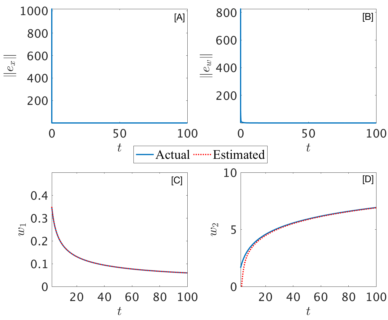
Figure 1: [A] State estimation error $e_{x}\triangleq\hat{x}-x$ of the nonlinear system in (60). [B] Unknown input estimation error. The convergence of the norm of $e_{w}\triangleq\hat{w}-w$ is illustrated. [C, D] Unknown inputs (blue) and their estimates (dashed red).

The response of the proposed observer is shown in Figure 1. Note that the unknown input $w_{2}$ is monotonically increasing, yet from Figure 1[C-D], we observe that the estimates of the unbounded unknown inputs are very accurate; this is to be expected since $\gamma$ is small.

7 Conclusions

This paper provides an LMI based approach to the design of observers for estimating the state and unknown exogenous input for a wide range of nonlinear systems. The resulting input-output system from exogenous input to estimation error is $\mathcal{L}_{2}$ stable with a gain that can be pre-specified and computed via standard toolboxes.

References

[1]
A. Teixeira, “Toward cyber-secure and resilient networked control systems,”
Ph.D. dissertation, KTH Royal Institute of Technology, 2014.
[2]
A. Chakrabarty, R. Ayoub, S. H. Żak, and S. Sundaram, “Delayed unknown
input observers for discrete-time linear systems with guaranteed
performance,” Systems & Control Letters, vol. 103, pp. 9–15, 2017.
[3]
J.-Y. Keller and M. Darouach, “Two-stage Kalman estimator with unknown
exogenous inputs,” Automatica, vol. 35, no. 2, pp. 339–342, 1999.
[4]
K. Khémiri, F. Hmida, J. Ragot, and M. Gossa, “Novel optimal recursive
filter for state and fault estimation of linear stochastic systems with
unknown disturbances,” International Journal of Applied Mathematics
and Computer Science, vol. 21, no. 4, pp. 629–637, 2011.
[5]
X. Zhang, M. M. Polycarpou, and T. Parisini, “Fault diagnosis of a class of
nonlinear uncertain systems with lipschitz nonlinearities using adaptive
estimation,” Automatica, vol. 46, no. 2, pp. 290–299, 2010.
[6]
T. Floquet, C. Edwards, and S. K. Spurgeon, “On sliding mode observers for
systems with unknown inputs,” International Journal of Adaptive
Control and Signal Processing, vol. 21, no. 8-9, pp. 638–656, 2007.
[7]
L. Fridman, Y. Shtessel, C. Edwards, and X.-G. Yan, “Higher-order sliding-mode
observer for state estimation and input reconstruction in nonlinear
systems,” International Journal of Robust and Nonlinear Control,
vol. 18, no. 4-5, pp. 399–412, 2008.
[8]
A. Chakrabarty, S. H. Żak, and S. Sundaram, “State and unknown input
observers for discrete-time nonlinear systems,” in Proc. of the IEEE
55th Conference on Decision and Control (CDC), 2016, pp. 7111–7116.
[9]
W. Chen and M. Saif, “Observer-based strategies for actuator fault detection,
isolation and estimation for certain class of uncertain nonlinear systems,”
IET Control Theory & Applications, vol. 1, no. 6, pp. 1672–1680,
2007.
[10]
A. Zemouche, M. Boutayeb, and G. I. Bara, “Observers for a class of Lipschitz
systems with extension to performance analysis,”
Systems & Control Letters, vol. 57, no. 1, pp. 18–27, 2008.
[11]
A. Zemouche, R. Rajamani, B. Boulkroune, H. Rafaralahy, and M. Zasadzinski,
“ circle observer design for Lipschitz nonlinear
systems with enchanced LMI conditions,” in 2016 American Control
Conference, 2016, pp. 131–136.
[12]
F. Bejarano, W. Perruquetti, T. Floquet, and G. Zheng, “State reconstruction
of nonlinear differential-algebraic systems with unknown inputs,” in
51st Annual Conference on Decision and Control (CDC), 2012, pp.
5882–5887.
[13]
W. Chen and M. Saif, “Unknown input observer design for a class of nonlinear
systems: an LMI approach,” in American Control Conference, 2006, pp.
439–463.
[14]
Q. P. Ha and H. Trinh, “State and input simultaneous estimation for a class of
nonlinear systems,” Automatica, vol. 40, no. 10, pp. 1779–1785,
2004.
[15]
M. Witczak, M. Buciakowski, V. Puig, D. Rotondo, and F. Nejjari, “An LMI
approach to robust fault estimation for a class of nonlinear systems,”
International Journal of Robust and Nonlinear Control, vol. 26, no. 7,
pp. 1530–1548, 2016.
[16]
J.-P. Barbot, M. Fliess, and T. Floquet, “An algebraic framework for the
design of nonlinear observers with unknown inputs,” in 46th IEEE
Conference on Decision and Control, 2007, pp. 384–389.
[17]
A. Zemouche and M. Boutayeb, “Nonlinear-Observer-Based
Synchronization and Unknown Input Recovery,” IEEE Transactions on
Circuits and Systems I: Regular Papers, vol. 56, no. 8, pp. 1720–1731,
2009.
[18]
A. Chakrabarty, M. J. Corless, G. T. Buzzard, S. H. Zak, and A. E. Rundell,
“Sufficient conditions for exogeneous input estimation in nonlinear
systems,” in Proc. of the American Control Conference (ACC), 2016,
pp. 103–108.
[19]
A. Chakrabarty, E. Fridman, S. H. Żak, and G. T. Buzzard, “State and
unknown input observers for nonlinear systems with delayed measurements,”
Automatica, vol. 95, pp. 246–253, 2018.
[20]
J. Su, H. Ma, W. Qiu, and Y. Xi, “Task-independent robotic uncalibrated
hand-eye coordination based on the extended state observer,” IEEE
Transactions on Systems, Man, and Cybernetics, Part B (Cybernetics),
vol. 34, no. 4, pp. 1917–1922, 2004.
[21]
H. Liu and S. Li, “Speed control for pmsm servo system using predictive
functional control and extended state observer,” IEEE Transactions on
Industrial Electronics, vol. 59, no. 2, pp. 1171–1183, 2012.
[22]
J. Wang, S. Li, J. Yang, B. Wu, and Q. Li, “Extended state observer-based
sliding mode control for pwm-based dc–dc buck power converter systems with
mismatched disturbances,” IET Control Theory & Applications, vol. 9,
no. 4, pp. 579–586, 2015.
[23]
Y. Xia, Z. Zhu, M. Fu, and S. Wang, “Attitude tracking of rigid spacecraft
with bounded disturbances,” IEEE Transactions on Industrial
Electronics, vol. 58, no. 2, pp. 647–659, 2011.
[24]
B. A. Francis and W. M. Wonham, “The internal model principle of control
theory,” Automatica, vol. 12, no. 5, pp. 457–465, 1976.
[25]
C. Johnson, “Accomodation of external disturbances in linear regulator and
servomechanism problems,” IEEE Transactions on automatic control,
vol. 16, no. 6, pp. 635–644, 1971.
[26]
S. Li, J. Yang, W.-H. Chen, and X. Chen, “Generalized extended state observer
based control for systems with mismatched uncertainties,” IEEE
Transactions on Industrial Electronics, vol. 59, no. 12, pp. 4792–4802,
2012.
[27]
A. A. Godbole, J. P. Kolhe, and S. E. Talole, “Performance analysis of
generalized extended state observer in tackling sinusoidal disturbances,”
IEEE Transactions on Control Systems Technology, vol. 21, no. 6, pp.
2212–2223, 2013.
[28]
X. Wei and N. Chen, “Composite hierarchical anti-disturbance control for
nonlinear systems with dobc and fuzzy control,” International Journal
of Robust and Nonlinear Control, vol. 24, no. 2, pp. 362–373, 2014.
[29]
B. Açıkmeşe and M. Corless, “Observers for systems with
nonlinearities satisfying incremental quadratic constraints,”
Automatica, vol. 47, no. 7, pp. 1339–1348, 2011.
[30]
A. Chakrabarty, M. J. Corless, G. T. Buzzard, S. H. Żak, and A. E. Rundell,
“State and unknown input observers for nonlinear systems with bounded
exogenous inputs,” IEEE Transactions on Automatic Control, vol. 62,
no. 11, pp. 5497–5510, 2017.
[31]
M. Corless and J. Tu, “State and Input Estimation for a Class of Uncertain
Systems,” Automatica, vol. 34, no. 6, pp. 757–764, 1998.
[32]
P. Tsiotras and M. Arcak, “Low-bias control of AMB subject to voltage
saturation: State-feedback and observer designs,” IEEE Transactions
on Control Systems Technology, vol. 13, no. 2, pp. 262–273, 2005.