Critical jammed phase of the linear perceptron

Abstract

Criticality in statistical physics naturally emerges at isolated points in the phase diagram. Jamming of spheres is not an exception: varying density, it is the critical point that separates the unjammed phase where spheres do not overlap and the jammed phase where they cannot be arranged without overlaps. The same remains true in more general constraint satisfaction problems with continuous variables (CCSP) where jamming coincides with the (protocol dependent) satisfiability transition point. In this work we show that by carefully choosing the cost function to be minimized, the region of criticality extends to occupy a whole region of the jammed phase. As a working example, we consider the spherical perceptron with a linear cost function in the unsatisfiable (UNSAT) jammed phase and we perform numerical simulations which show critical power laws emerging in the configurations obtained minimizing the linear cost function. We develop a scaling theory to compute the emerging critical exponents.

Introduction – The jamming transition of spheres is a critical point Liu and Nagel (2010). At jamming, spheres form an isostatic network Tkachenko and Witten (1999) where the number of contacts between them equals exactly the total number of degrees of freedom. Furthermore, the distributions of forces and gaps (i.e. distances) between particles display power laws Wyart (2012); Lerner et al. (2013); Mueller and Wyart (2015); Charbonneau et al. (2015) which play a central role in the mechanical and rheological properties of such systems. In Charbonneau et al. (2014a, b) the corresponding critical exponents have been computed from the solution of the hard sphere model in infinite dimension. In this analysis the jamming transition is thought of as the infinite pressure limit of hard sphere glassy states.

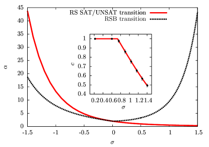
Figure 1: The phase diagram of the spherical perceptron with linear cost function. The $y$-axis represents the density of constraints $\alpha=M/N$ while the $x$-axis is the control parameter $\sigma$ that defines the gap variables, see Eq. (1). The red solid line is the SAT/UNSAT (jamming) line (computed under the replica symmetric approximation, exact only for $\sigma>0$). Below this line the model is SAT/unjammed and one can find zero energy configurations. Above, the problem is UNSAT/jammed and the energy is positive. Above the black dashed line replica symmetry spontaneously breaks down: below this line the problem is convex while above the energy landscape is glassy with many local minima with critical properties. The jamming line lies in the RS region for $\sigma>0$ and in the RSB region for $\sigma<0$. Inset: The density of contacts $c$ for $\alpha=5$ as a function of $\sigma$. The red line corresponds to the theoretical prediction. We have hypostaticity $c<1$ in the RS phase and isostaticity, i.e. $c=1$ in the RSB phase. The dots come from numerical simulations with $N=1024$ at $\alpha=5$.

Upon compression, hard sphere glasses undergo a Gardner transition Kurchan et al. (2013); the glass basins of configurations split into a ’fractal landscape’ of just marginally stable metastable states, described by full replica symmetry breaking (RSB) Mézard et al. (1987), with soft excitations and divergent susceptibilities. Within this mean-field scenario, these excitations are responsible for the anomalous rheological response of amorphous solids Biroli and Urbani (2016); Franz and Spigler (2017); Jin et al. (2018); Jin and Yoshino (2017); Rainone et al. (2015). In the jamming limit this landscape marginality gives rise to the power laws observed in the gaps and forces distributions and predicts the mechanical properties of amorphous jammed packings.

Subsequently, it has been argued Franz and Parisi (2016); Franz et al. (2015, 2017) that the jamming transition can be thought of as a special case of a satisfiability transition for constraint satisfaction problems Moore and Mertens (2011) with continuous variables (CCSP). In a generic CCSP one seeks configurations of variables that satisfy a set of constraints. From this viewpoint, jamming is the (protocol dependent) point that separates a satisfiable (SAT) unjammed phase, where the spheres can be arranged to satisfy the non-overlapping constraints, from an unsatisfiable (UNSAT) or jammed phase, where some constraints are violated and spheres overlap. In this way, one can generalize the problem of jamming to other situations. The simplest one is borrowed from machine learning and is a non-convex twist of the perceptron classifier Engel and Van den Broeck (2001). In Franz and Parisi (2016) it has been argued that at the satisfiability transition point (meaning at jamming) this CCSP displays analogous power law distributions of gaps and forces whose critical exponents coincide with the ones of spheres. Non-trivial generalizations of the perceptron Franz et al. (2018); Yoshino (2018) retain the same critical behavior.

However, the criticality of the gaps and forces distributions both in spheres and in the perceptron is generically attributed to the emergence of jamming and should disappear in the jammed/UNSAT phase. This is supported by analytical computations in the perceptron problem with harmonic cost function and by numerical simulations on harmonic soft spheres.

In this work we show that this is not always the case: changing the potential or cost function from harmonic to linear, we find jamming criticality in an extensive region of the UNSAT/jammed phase, far away from jamming.

We consider the UNSAT/jammed phase of the simplest CCSP, the spherical perceptron model, and we look at local minima of the linear cost function (instead of the harmonic one). We show that even far from jamming, in an extensive region of the phase diagram, the landscape induced by this cost function is non-convex and composed by metastable minima which are all jamming-critical. Indeed, for these minima the positive and negative gaps distributions display power law divergences for small argument: surprisingly, the critical exponents describing these power laws coincide with the ones of the jamming transition. Moreover, we find that this behavior is associated with isostaticity: even when the model is in the UNSAT phase, there is an extensive number of marginally satisfied constraints, i.e. constraints that are right at the border of satisfaction (like perfectly touching spheres). The jamming-critical phase appears when the number of marginally satisfied constraints equals the number of degrees of freedom of the system which becomes therefore isostatic.

The spherical perceptron with linear cost function has been studied in Griniasty and Gutfreund (1991); Györgyi (2001); Majer et al. (1993) where the phase diagram was obtained using the replica method and studied at the so-called replica symmetric level in Griniasty and Gutfreund (1991). While it was known that RSB is needed in the UNSAT/jammed phase systematic studies beyond 1RSB Majer et al. (1993); Györgyi and Reimann (1997, 2000) were not undertaken. Here we show that the emergence of RSB in the UNSAT phase is related to the emergence of jamming-like criticality.

The model – The spherical perceptron is an optimization problem defined through an $N$-dimensional vector $\underline{w}$ on the $N$-dimensional hypersphere $|\underline{w}|^{2}=N$ and by a set of $M=\alpha N$ $N$-dimensional random vectors $\{\underline{\xi}^{\mu}\}$ whose components are i.i.d. Gaussian random variables with zero mean and unit variance. For each of these vectors one defines the gap $h_{\mu}$ by

$$h_{\mu}=\frac{1}{\sqrt{N}}\underline{\xi}^{\mu}\cdot\underline{w}-\sigma\>.$$ (1)

We say that a gap $h_{\mu}$ is (i) satisfied if $h_{\mu}>0$, (ii) marginally satisfied if $h_{\mu}=0$ and (iii) unsatisfied if $h_{\mu}<0$. The variables $\sigma$ and $\alpha$ are control parameters. One can define an energy or cost function associated with the unsatisfied gaps as

$$H[\underline{w}]=\frac{1}{p}\sum_{\mu=1}^{\alpha N}|h_{\mu}|^{p}\theta(-h_{\mu})\>$$ (2)

and study its minima. Eq. (2) depends on a parameter $p$ that sets the strength of the cost when gap variables are unsatisfied. The harmonic perceptron corresponds to $p=2$ and has been studied in Franz et al. (2015, 2017). Here we set $p=1$ which defines the linear cost function. This cost function is not very used in soft matter systems but it is common in the machine learning literature where it is called hinge loss and plays an important role in Support Vector Machines Zhu et al. (2004). Furthermore, the case $p=1$ marks the boundary where $H$ passes from a convex ($p>1$) to a non-convex ($p<1$) function of each of the $h_{\mu}$’s. We stress however that the convexity of $H$ in the $h_{\mu}$’s does not necessarily imply convexity of $H$ in the variables $\underline{w}$ that live on the hypersphere: the loss of convexity is indeed associated with glassiness.

The phase diagram of the spherical perceptron with linear cost function was obtained for $\sigma>0$ in Griniasty and Gutfreund (1991) (see also Majer et al. (1993)) and is redrawn in Fig. 1 in terms of the control parameters $\sigma$ and $\alpha$. It contains two regions separated by the SAT/UNSAT transition line (red line in Fig. 1). Below this line the problem is SAT (or unjammed) meaning that with probability one, for $N\rightarrow\infty$, there are configurations of $\underline{w}$ for which the cost function is strictly zero, i.e. the gaps $h_{\mu}$ are satisfied for all $\mu=1,\ldots,\alpha N$. Conversely, above this line the cost function is positive and an extensive number of gaps are unsatisfied: this is the UNSAT/jammed phase. In Fig. 1 we plot also the de Almeida-Thouless (RSB) line De Almeida and Thouless (1978) (dashed black line): below this line and in the UNSAT phase, the energy landscape is effectively convex and the linear cost function has a unique global minimum. Above this line, convexity is lost and multiple metastable minima emerge. We are interested in studying the properties of these local minima.

Numerical Simulations – Local minima of the linear cost function turn out to be non-analytic angular points determined by the intersection of hyperplanes. We smooth out the singularity at $h_{\mu}=0$ and define a regularized cost function as

$$\begin{split}H_{\varepsilon}[\underline{w}]&=\sum_{\mu=1}^{\alpha N}\left|h_{\mu}+\frac{\varepsilon}{2}\right|\theta(-h_{\mu}-\varepsilon)+\frac{\zeta}{4}(|\underline{w}|^{2}-N)^{2}\\ &+\frac{1}{2\varepsilon}\sum_{\mu=1}^{\alpha N}h_{\mu}^{2}\theta(\varepsilon+h_{\mu})\theta(-h_{\mu})\\ \end{split}$$ (3)

where $\varepsilon>0$ and $\zeta$ is an arbitrary large constant needed to enforce the spherical constraint $|\underline{w}|^{2}=N$. We implemented the numerical minimization of $H_{\varepsilon}[\underline{w}]$ using the routine BFGS Fletcher (2013) of the SciPy library Jones et al. (01). For every $\varepsilon$, the algorithm reaches a local minimum. In order to describe the properties of the linear cost function, we need to study the minima when $\varepsilon\rightarrow 0^{+}$. Therefore, we consider a decreasing sequence of values of $\varepsilon$ and minimize the cost function at each step (see SM for details). We observe that for $\varepsilon$ small enough there is an extensive fixed set of gaps in the interval ${\cal D}=[-\varepsilon,0]$. Decreasing $\varepsilon$, these gaps remain in ${\cal D}$, indicating that for $\varepsilon\rightarrow 0^{+}$ they become marginally satisfied: we call them contacts in analogy with sphere packings. We define the empirical distribution of gaps as $\rho(h)=\overline{\frac{1}{M}\sum_{\mu=1}^{M}\delta(h-h_{\mu})}$ where the average is taken over many different realizations of the random vectors $\{\underline{\xi}^{\mu}\}$. Therefore, for $\varepsilon\rightarrow 0^{+}$ $\rho(h)$ contains a Dirac delta at $h=0$. Calling ${\cal I}_{\cal D}$ the total number of contacts, we can define an isostaticity index $c={\cal I}_{\cal D}/N$. In the inset of Fig. 1 we plot $c$ as a function of $\sigma$ for $\alpha=5$. When replica symmetry is unbroken (RS),we find $c<1$ and we say that minima are hypostatic. Conversely, when the minimization is carried in the RSB region we find $c=1$ and therefore we say that minima are isostatic.

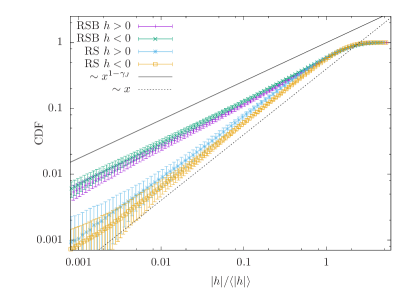
Figure 2: The cumulative distribution function (CDF) of both strictly positive and strictly negative gaps for $N=1024$ and $\alpha=5$. We compare the distributions in the UNSAT-RSB and UNSAT-RS regions. The RSB data refer to minima at an average energy $H/N=1.01\pm 0.02$ and the corresponding value of $\sigma$ is $\sigma=0.219\pm 0.004$. Both positive and negative gaps’ distributions are compatible with a power law at small argument with exponent $1-\gamma_{J}\simeq 0.59$ (black full line). The RS data refer to minima with $H/N=2.540\pm 0.013$ and $\sigma=0.757\pm 0.010$. One sees there a linear behavior of the CDF, implying a positive probability density function in the origin.

Once the contacts are identified we construct the statistics of strictly positive and negative gaps. We study what happens to $\rho(h)$ when $h\rightarrow 0^{\pm}$. In the RS-UNSAT phase, $\rho(h\rightarrow 0^{\pm})\rightarrow A_{\pm}$ being $A_{\pm}$ two positive non-universal constants that depend on the control parameters. In the RSB region instead we observe that $\rho(h\rightarrow 0^{\pm})\sim|h|^{-\gamma_{\pm}}$ where $\gamma_{\pm}$ are two critical exponents. In Fig. 2, we plot the cumulative distributions of both positive and negative gaps for minima with an average energy of $\langle H\rangle/N=1.01\pm 0.02$, therefore far away from the jamming transition. Both distributions display a non-trivial power law for small argument. The critical exponents $\gamma_{\pm}$ are very close to each other and have numerical value $\gamma_{+}\approx\gamma_{-}\approx 0.41$ which is compatible with the critical exponent $\gamma_{J}$ that controls the positive gaps distribution at jamming transition Charbonneau et al. (2014a). Moreover, we can obtain the virtual forces $\hat{f}$ associated to contacts Franz and Parisi (2016). These are defined as the Lagrange multipliers needed to enforce that the corresponding gaps are identically zero . Their empirical distribution is defined as $\rho_{f}(\hat{f})=\overline{\frac{1}{cN}\sum_{i\in{\cal D}}\delta(\hat{f}-\hat{f}_{i})}$ and has support in $[0,1]$. We find that while in the convex phase $\rho_{f}(\hat{f})$ is regular at both edges, in the RSB phase it becomes critical, with pseudogaps close to both edges of its support, $\rho_{f}(\hat{f})\sim\hat{f}^{\theta}$ and $\rho_{f}(\hat{f})\sim(1-\hat{f})^{\theta^{\prime}}$ for $\hat{f}\sim 0^{+}$ and for $\hat{f}\sim 1^{-}$ respectively. In Fig. 3, we plot the cumulative distribution of forces both as a function of $\hat{f}$ and $1-\hat{f}$ as obtained from simulations: we observe two power laws with exponents $\theta\simeq\theta^{\prime}\simeq 0.42$, again compatible with the critical exponent $\theta_{J}$ that controls the distribution of small forces at jamming.

Therefore numerical simulations show that when the energy minimization is carried out in the RSB-UNSAT phase, there are three classes of small gaps: an isostatic set of gaps that are identically zero, and two sets of positive and negative gaps that accumulate around zero. Furthermore, the marginally satisfied gaps are associated to a critical distribution of virtual forces. Unlike for the harmonic case, here scaling behavior emerges even in the UNSAT phase far from jamming.

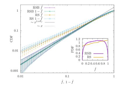
Figure 3: The CDF of the virtual forces presented as a function of both $\hat{f}$ and $1-\hat{f}$ for the same parameters as in fig. 2. In the RSB phase the distribution of forces vanishes as a power law both in $\hat{f}=0$ and in $\hat{f}=1$ (purple line in the inset) and both powers are compatible with $\theta_{J}\simeq 0.42$ corresponding to a CDF with a power $1.42$. In the RS region the behavior is linear and the PDF is finite at both edges of its support (yellow line in the inset).

Theory – We analyze the thermodynamic phase diagram of the model using the replica method. Similarly to the case of the jamming transition in spheres and non-convex perceptron, the UNSAT critical phase is associated with scaling behavior that controls the universality of the gaps and forces distributions. However, in the case of the jamming transition there is a single scaling region that describes small positive gaps and forces. Instead, in the present case we also have two additional power laws describing small negative gaps and virtual forces close to one. This corresponds to the emergence of an additional scaling region. Both regions can be theoretically identified from the replica analysis. Here we sketch the main steps, details are in the SM. The phase diagram and the properties of the model can be obtained by studying the zero temperature limit $\beta=1/T\rightarrow\infty$ of its free energy Gardner (1988)

$${\rm f}=-\frac{1}{\beta N}\overline{\ln\int{\mathrm{d}}\underline{w}\,{\mathrm{e}}^{-\beta H[\underline{w}]}}$$ (4)

where the overline stands for the average over the random vectors $\underline{\xi}^{\mu}$. The disorder average can be performed using the replica method Györgyi (2001); Franz et al. (2017). The RSB phase is described by the probability distribution of the overlap $q=\underline{w}_{1}\cdot\underline{w}_{2}/N$ between different configurations and is captured by the following PDEs Mézard et al. (1987); Sommers and Dupont (1984), valid for real values of $h$ and for $q$ in a interval $q\in[q_{m},q_{M}]\subset[0,1]$ determined self-consistently:

$$\begin{split}\frac{\partial m(q,h)}{\partial q}&=-\frac{1}{2}m^{\prime\prime}(q,h)-\frac{x(q)}{\lambda(q)}m(q,h)\left[1+m^{\prime}(q,h)\right]\\ \frac{\partial P(q,h)}{\partial q}&=\frac{1}{2}\left[P^{\prime\prime}(q,h)-2\frac{x(q)}{\lambda(q)}\left(P(q,h)m(q,h)\right)^{\prime}\right]\end{split}$$ (5)

where the primes indicate partial derivatives with respect to $h$ and the boundary conditions are given by

$$\begin{split}m(q_{M},h)&=(1-q_{M})\frac{\partial}{\partial h}\ln\gamma_{1-q_{M}}\star e^{-\beta|h|\theta(-h)}\\ P(q_{m},h)&=\gamma_{q_{m}}(h+\sigma)\>.\end{split}$$ (6)

$\gamma_{\Delta}$ is a Gaussian with zero mean and variance $\Delta$ and $\star$ stands for the convolution operation. The function $x(q)$ is directly related to the distribution of the overlap $q$ Mézard et al. (1987) and we have defined $\lambda(q)=1-q_{M}+\int_{q}^{q_{M}}\mathrm{d}p\;x(p).$ At large $\beta$, one can get the distribution of virtual forces and gaps from the solution of $P(q,h)$ in the limit $q\rightarrow 1$. We analyze Eqs. (10) in the $\beta\rightarrow\infty$ limit in the RSB-UNSAT phase and show that they admit a scaling solution which accounts for the power laws observed in numerical simulations. In the UNSAT phase, for $\beta\rightarrow\infty$ one has $q_{M}\rightarrow 1$. In the limit $0<1-q\ll 1$ two scaling regimes emerge for $m(q,h)$. One concerns the region $h=O(\sqrt{1-q})$, analogue to the one found at jamming Charbonneau et al. (2014a), and a new one associated to negative gaps for $h=-\hat{\lambda}(q)+O(\sqrt{1-q})$, where $\hat{\lambda}(q)=\lim_{\beta\rightarrow\infty}\beta\lambda(q)\simeq(1-q)^{(\kappa-1)/\kappa}\gg\sqrt{1-q}$ (being $\kappa<2$ a critical exponent). Therefore we can write

$$m(q,h)=\begin{cases}-\sqrt{1-q}{\cal M}_{+}\left(\frac{h}{\sqrt{1-q}}\right)&|h|\sim\sqrt{1-q}\\ -h+\sqrt{1-q}{\cal M}_{-}\left(\frac{h+\hat{\lambda}(q)}{\sqrt{1-q}}\right)&h+\hat{\lambda}(q)\sim\sqrt{1-q}.\end{cases}$$ (7)

It turns out that the two scaling functions are related by the symmetry relation ${\cal M}_{-}(t)=t+{\cal M}_{+}(-t)$. Moreover, we find that the scaling function ${\cal M}_{+}$ satisfies the same equation that appear at critical jamming transitions Charbonneau et al. (2014b); Franz et al. (2017). At the same time, the function $P(q,h)$ admits the scaling form

$$P(q,h)=\begin{cases}p_{+}(h)&h\gg\sqrt{1-q}\\ (1-q)^{-a/\kappa}p_{0}\left(\frac{h}{\sqrt{1-q}}\right)&h\sim\sqrt{1-q}\\ \hat{\lambda}(q)^{-1}p_{-}(h\hat{\lambda}(q)^{-1})&-h\sim\hat{\lambda}(q)\\ (1-q)^{-a/\kappa}\tilde{p}_{0}\left(\frac{h+\hat{\lambda}(q)}{\sqrt{1-q}}\right)&|h+\hat{\lambda}(q)|\sim\sqrt{1-q}\\ \tilde{p}_{+}(h+\hat{\lambda}(q))&h+\hat{\lambda}(q)\ll-\sqrt{1-q}.\end{cases}$$ (8)

The scaling functions $p_{+}(t)$ and $\tilde{p}_{+}(t)$ control respectively the distribution of small positive and negative gaps. Furthermore $\tilde{p}_{0}(t)=p_{0}(-t)$ and $p_{0}(t)$ satisfies again a scaling equation that is exactly the same as the one appearing at critical jamming Charbonneau et al. (2014b); Franz et al. (2017). This analysis implies that the exponents verify: $\gamma_{+}=\gamma_{-}=\gamma_{J}$ and $\theta=\theta^{\prime}=\theta_{J}$ being $\gamma_{J}\simeq 0.41$ and $\theta_{J}\simeq 0.42$ the critical exponents controlling the gaps and forces distributions at the jamming point of hard spheres. Finally the nature of the scaling solution implies that the distribution of gaps has an isostatic delta peak of marginally satisfied gaps, so we get

$$\begin{split}\rho(h)&\sim\rho_{+}h^{-\gamma}\theta(h)+\rho_{-}(-h)^{-\gamma}\theta(-h)+\frac{1}{\alpha}\delta(h)\ \ h\rightarrow 0\end{split}$$ (9)

with $\rho_{+}$ and $\rho_{-}$ two positive constants.

Conclusions – We have analyzed the properties of the UNSAT phase of the spherical perceptron with linear cost function. In the RS phase the landscape is effectively convex and the global minimum is not critical and hypostatic. When instead the minimization is carried out in the RSB phase, we find that local minima are jamming-critical. They are described by an isostatic number of contacts and the distributions of gaps and virtual forces follow power laws whose exponents are the same as the ones characterizing jamming of hard spheres. We have proposed a scaling solution of the RSB equations that agrees with the emerging criticality. There are two clear future directions. First, it will be interesting to understand what happens to the model if we change the cost function to a non-convex function of the gaps (i.e. $p<1$ in Eq.(2)). Furthermore, it will be interesting to study linear cost functions in other CCSPs, and see if this leads to universal critical jammed phases as it happens in the perceptron. We expect that that this property is generic within mean-field, and our scaling solution extends to high dimensional spheres, multilayer neural nets etc. Franz et al. (2018); Yoshino (2018). More interesting are problems that are not mean-field in nature. For finite dimensional spheres the critical exponents of jamming have been shown to be independent on spatial dimension within numerical accuracy Charbonneau et al. (2015). It would be interesting to investigate if the same property holds for the jammed phase of linear soft spheres. We are working in this direction. This may provide a finite dimensional physical system with an extended jamming-critical phase where RSB effects could be tested.

Appendix A Dictionary between continuous constraint satisfaction problems and jamming of spheres

In this section we recall the dictionary between jamming of spheres and continuous constraint satisfaction problems with excluded volume constraints. This mapping has been first presented in Franz et al. (2015, 2017).

• CCSP. Continuous constraint satisfaction problem with excluded volume constraints can be defined in an abstract way. One considers first a vector $\underline{w}\in{\rm I\!R}^{N}$ and a set of $M=\alpha N$ functions $h_{\mu}(\underline{w})\in{\rm I\!R}$ indexed by $\mu=1,\ldots,M$. Each function $h_{\mu}(\underline{w})$ is called gap. The constraint satisfaction problem is defined by asking a configuration of $\underline{w}$ that satisfies all the constraints $h_{\mu}(\underline{w})\geq 0$. If the problem cannot be satisfied one can define an optimization problem by asking to find a configuration of $\underline{w}$ that minimizes a cost function. Therefore in general one can define a cost function $H=\frac{1}{p}\sum_{\mu}|h_{\mu}|^{p}\theta(-h_{\mu})$ where the power $p$ sets the magnitude of the contribution of the negative gaps to the total cost. The satisfiable (SAT) phase corresponds to an assignment where $H=0$ while we have $H>0$ in the unsatisfiable (UNSAT) phase. The boundary between the two phases is the SAT/UNSAT transition and will be generically referred to as the jamming point. The precise location of this point as a function of the control parameters of the problem may depend on the precise protocol used to obtain solutions. Marginally satisfied gaps are defined by $h_{\mu}(\underline{w})=0$.

• Spheres. In this case the degrees of freedom of the problem are the positions of $N$ spheres in ${\rm I\!R}^{d}$ denoted by $\{\underline{x}_{i}\in{\rm I\!R}^{d}\}_{i=1,\ldots,N}$. The gap variables are defined for each couple of spheres as $h_{ij}=|\underline{x}_{i}-\underline{x}_{j}|-\sigma_{ij}$ where $\sigma_{ij}=r_{i}+r_{j}$, being $\{r_{i}\}_{i=1,\ldots,N}$ the values of the radii of the spheres. The constraint satisfaction problem is defined by asking to find a configuration of the spheres such that $h_{ij}\geq 0$ for all couples $\{ij\}$. A contact between two spheres $i$ and $j$ appears if $h_{ij}=0$ which corresponds to a marginally satisfied gap. The jamming point separates the unjammed (SAT) phase where it is possible to find a SAT configuration for the positions of the spheres, from the jammed (UNSAT) phase where the spheres overlap and an extensive number of gaps are negative. In the jammed phase one can define a cost function $H=\frac{1}{p}\sum_{i<j}|h_{ij}|^{p}\theta(-h_{ij})$. For $p=2,2.5$ one obtain harmonic or Hertzian spheres respectively.

• Spherical perceptron. The degrees of freedom of the spherical perceptron problem are enclosed in an $N$-dimensional vector $\underline{w}\in{\rm I\!R}^{N}$ subjected to stay on the sphere $|\underline{w}|^{2}=N$. One then introduces a set of $M=\alpha N$ random vectors $\{\underline{\xi}^{\mu}\in{\rm I\!R}^{N}\}_{\mu=1,\ldots,M}$ whose components are $i.i.d.$ random Gaussian variables with zero mean and unit variance. Given these random vectors the gaps are defined by $h_{\mu}(\underline{w})=\underline{\xi}^{\mu}\cdot\underline{w}/\sqrt{N}-\sigma$ being $\sigma$ a control parameter in the problem playing a role similar to the diameter in spheres. The constraint satisfaction problem requires to find a configuration of $\underline{w}$ such that $h_{\mu}\geq 0$ for all $\mu=1,\ldots,M$. In the UNSAT phase, where such configurations cannot be found, one can define an optimization problem by asking to find configurations of $\underline{w}$ that minimize a cost function given by $H=\frac{1}{p}\sum_{\mu}|h_{\mu}|^{p}\theta(-h_{\mu})$. In the present paper we have set $p=1$ that defines the linear cost function but one can also study the harmonic case and this has been done in Franz et al. (2015, 2017). Again, marginally satisfied gaps, analogous to contacts between spheres, correspond to $h_{\mu}=0$.

Appendix B Scaling solution of the fullRSB equations

Here we give the details about the scaling solution of the fullRSB equations we have proposed in the main text to understand the the critical exponents appearing in the numerical simulations. Note that in the glassy phase the numerical minimization does not output the ground state of the system. Therefore we should in principle not expect to have a correspondence between the thermodynamic computation and the numerical findings. Nevertheless we will show that the scaling solution of the RSB equations give rise to critical exponents which are compatible with the numerical findings. The same phenomenon happens at jamming and this is another manifestation of universality. The deep reasons for this is still a matter of active research.

We assume that in the UNSAT RSB region, replica symmetry is broken in a continuous way, at least for $q\rightarrow 1$ (see below). This property implies a proliferation of metastable states in the vicinity of the ground state. The basic assumption to apply this theory off equilibrium is that this proliferation also happens around local minima reached by local minimization algorithms.

The fullRSB solution of the perceptron problem can be derived following similar steps as in Franz et al. (2017) and changing the cost function from harmonic to linear. The free energy of the model can be obtained through a saddle point for an order parameter that is the overlap distribution between different minima in the free energy landscape. This quantity is encoded in the function $x(q)$ defined in the interval $[q_{m},q_{M}]$ where the extrema of the interval, $0<q_{m}<q_{M}\leq 1$ Mézard et al. (1987) have to be determined self-consistently together with the function $x(q)$. The saddle point equations for $x(q)$ can be written in terms of two auxiliary functions $m(q,h)$ and $P(q,h)$. In particular one can show that $P(q,h)$ for $q\rightarrow q_{M}$ encodes the properties of the gaps and forces distributions Franz et al. (2017). The functions $m(q,h)$ and $P(q,h)$ verify the following PDE’s:

$$\begin{split}\dot{m}(q,h)&=-\frac{1}{2}m^{\prime\prime}(q,h)-\frac{x(q)}{\lambda(q)}m(q,h)\left[1+m^{\prime}(q,h)\right]\\ \dot{P}(q,h)&=\frac{1}{2}\left[P^{\prime\prime}(q,h)-2\frac{x(q)}{\lambda(q)}\left(P(q,h)m(q,h)\right)^{\prime}\right]\end{split}$$ (10)

where we have denoted with the dot the derivative w.r.t. $q$ and with the prime the derivative w.r.t. $h$. The boundary conditions of Eqs. (10) are given by

$$\begin{split}m(q_{M},h)&=(1-q_{M})\frac{\partial}{\partial h}\ln\gamma_{1-q_{M}}\star e^{-\beta|h|\theta(-h)}\\ P(q_{m},h)&=\gamma_{q_{m}}(h+\sigma)\>.\end{split}$$ (11)

We want to analyze the behavior of these equations in the zero temperature limit $T\rightarrow 0$, $\beta\rightarrow\infty$. Therefore we introduce the following re-scaled functions

$$y(q)=\beta x(q)\ \ \ \ \ \ \ \ \ \ \hat{\lambda}(q)=\beta(1-q_{M})+\int_{q}^{q_{M}}\mathrm{d}py(p)\>.$$ (12)

The asymptotic behavior of $m(q_{M},h)$ for $q_{M}\rightarrow 1$ is given by

$$m(q_{M},h)=\begin{cases}0,\hskip 34.14322pt\text{for }h>0\\ -h,\qquad\text{for }-\beta(1-q_{M})\ll h\ll 0\\ \beta(1-q_{M}),\quad\text{for }h\ll-\beta(1-q_{M})\\ \end{cases}$$ (13)

This form suggests to look for an asymptotic solution for the equation for $m(q,h)$ given by

$$m(q,h)=\begin{cases}0,\hskip 34.14322pt\text{for }h>0\\ -h,\qquad\text{for }-\hat{\lambda}(q)\ll h\ll 0\\ \hat{\lambda}(q),\quad\text{for }h\ll-\hat{\lambda}(q)\\ \end{cases}$$ (14)

Note that Eq. (14) agrees with the boundary condition of Eq. (13) and asymptotically satisfies the Parisi equation for $m(q,h)$.

We now want to study the behavior of the solution of Eqs. (10) in the limit $T\rightarrow 0$, where $q_{M}\rightarrow 1$, and then $q\rightarrow 1$. However we will focus on the scaling limit where $1-q_{M}\ll 1-q\ll 1$. In this regime, based on Eq. (14), we can guess the following scaling form

$$m(q,h)=\begin{cases}-\sqrt{1-q}\,{\cal M}_{+}\left(\frac{h}{\sqrt{1-q}}\right)&|h|\sim\sqrt{1-q}\\ -h+\sqrt{1-q}\,{\cal M}_{-}\left(\frac{h+\hat{\lambda}(q)}{\sqrt{1-q}}\right)&h+\hat{\lambda}(q)\sim\sqrt{1-q}\end{cases}$$ (15)

with the boundary conditions:

$$\begin{split}&{\cal M}_{+}(t\rightarrow\infty)={\cal M}_{-}(t\rightarrow\infty)=0\\ &{\cal M}_{+}(t\rightarrow-\infty)={\cal M}_{-}(t\rightarrow-\infty)=t\>.\end{split}$$ (16)

These boundary conditions agree with Eq. (14). In order to compute the scaling equations for ${\cal M}_{\pm}$ we need to consider a scaling form for $y(q)$. We assume that

$$\begin{split}&y(q)\sim y_{\chi}(1-q)^{-\frac{1}{\kappa}}\\ &1-q_{M}\sim\chi T^{\kappa}\end{split}$$ (17)

so that for $1-q_{M}\ll 1-q\ll 1$ we get

$$\frac{y(q)}{\hat{\lambda}(q)}\sim\frac{\kappa-1}{\kappa}\frac{1}{1-q}\>.$$ (18)

Plugging this result inside the Parisi equation for $m(q,h)$ and using the scaling ansatz of Eq. (15) we get the following scaling equations for ${\cal M}_{\pm}$

$$\begin{split}&\begin{cases}&{\cal M}_{+}(t)-t{\cal M}_{+}(t)={\cal M}_{+}^{\prime\prime}(t)+2\frac{\kappa-1}{\kappa}{\cal M}_{+}(t)\left[1-{\cal M}_{+}^{\prime}(t)\right]\\ &{\cal M}_{+}(t\rightarrow\infty)=0\qquad{\cal M}_{+}(t\rightarrow-\infty)=t\>.\end{cases}\\ &\begin{cases}&{\cal M}_{-}\left(t_{-}\right)-t_{-}\ {\cal M}_{-}\left(t_{-}\right)={\cal M}^{\prime\prime}_{-}\left(t_{-}\right)-2\frac{\kappa-1}{\kappa}\left[t_{-}-{\cal M}_{-}\left(t_{-}\right)\right]{\cal M}^{\prime}_{-}\left(t_{-}\right)\\ &{\cal M}_{-}(t\rightarrow\infty)=0\qquad{\cal M}_{-}(t\rightarrow-\infty)=t\>.\end{cases}\end{split}$$ (19)

The scaling equation for ${\cal M}_{+}$ coincides with the scaling equation found in the case of jamming of hard spheres and perceptron Charbonneau et al. (2014b); Franz et al. (2017) and therefore it has the same solution provided that the value of the exponent $\kappa$ coincides with the one appearing at the jamming transition (we will see that this is the case). Furthermore we can show that the solution of the equation for ${\cal M}_{-}$ can be obtained from ${\cal M}_{+}$ using a symmetry transformation. Indeed it is very easy to show that if ${\cal M}_{+}(t)$ is a solution of the corresponding scaling equation, then if we set ${\cal M}_{-}(t)$ to be

$${\cal M}_{-}(t)=t+{\cal M}_{+}(-t)$$ (20)

this satisfies its corresponding scaling equation. Note that the mapping in Eq. (20) preserves the boundary conditions for ${\cal M}_{-}(t)$ as it should. This tells that the scaling behavior of ${\cal M}_{\pm}$ can be reduced to just one function ${\cal M}_{+}(t)$ which then happens to be the same as the one controlling the jamming point of spheres Charbonneau et al. (2014b); Franz et al. (2017).

We now turn to the analysis of the PDE for $P(q,h)$. We consider the following scaling ansatz for $q\rightarrow 1$

$$P(q,h)=\begin{split}\begin{cases}p_{+}(h)&h>0\\ (1-q)^{-\frac{a}{\kappa}}\ p_{0}\left(\frac{h}{\sqrt{1-q}}\right)&|h|\sim\sqrt{1-q}\\ \hat{\lambda}(q)^{-1}\ p_{-}\left(h\hat{\lambda}(q)^{-1}\right)&-\hat{\lambda}(q)\ll h\ll-\sqrt{1-q}\\ (1-q)^{\frac{\tilde{a}}{\kappa}}\tilde{p}_{0}\left(\frac{h+\hat{\lambda}(q)}{\sqrt{1-q}}\right)&|h+\hat{\lambda}(q)|\sim\sqrt{1-q}\\ \tilde{p}_{+}(h)&h\ll-\hat{\lambda}(q)\end{cases}\end{split}$$ (21)

and we have introduced two additional exponents $a$ and $\tilde{a}$. The two scaling functions $p_{0}$ and $\tilde{p}_{0}$ live on the same window where the two scaling functions ${\cal M}_{\pm}$ are different from their boundary behavior. As at the jamming transition Charbonneau et al. (2014b), we can obtain the corresponding scaling equations by plugging the scaling ansatz into the equation for $P(q,h)$. In the regime where $|h|\sim\sqrt{1-q}$ we get

$$\frac{a}{\kappa}p_{0}(t)+\frac{1}{2}t\ p_{0}^{\prime}(t)=\frac{p_{0}^{\prime\prime}(t)}{2}+\frac{\kappa-1}{\kappa}\left[p_{0}(t)\mathcal{M}_{+}(t)\right]^{\prime}\>.$$ (22)

This equation coincides with the one for the corresponding $p_{0}(t)$ at the jamming Charbonneau et al. (2014b); Franz et al. (2017).

Instead, in the regime where $|h+\hat{\lambda}(q)|\sim\sqrt{1-q}$ we get that

$$\frac{\tilde{a}}{\kappa}\tilde{p}_{0}(t)+\frac{1}{2}t\ \tilde{p}_{0}^{\prime}(t)=\frac{\tilde{p}_{0}^{\prime\prime}(t)}{2}-\frac{\kappa-1}{\kappa}\left\{\tilde{p}_{0}(t)\left[-t+\mathcal{M}_{-}(t)\right]\right\}^{\prime}$$ (23)

The boundary conditions for Eqs. (22-23) are

$$\begin{split}&p_{0}(t\rightarrow\infty)\sim|t|^{-\gamma}\ \ \ \ \tilde{p}_{0}(t\rightarrow-\infty)\sim|t|^{-\gamma^{\prime}}\\ &p_{0}(t\rightarrow-\infty)\sim|t|^{\theta}\ \ \ \ \tilde{p}_{0}(t\rightarrow\infty)\sim|t|^{\theta^{\prime}}\\ \end{split}$$ (24)

which imply the matching conditions

$$\begin{split}p_{+}(t\rightarrow 0^{+})\sim t^{-\gamma}\ \ \ \ \tilde{p}_{+}(t\rightarrow 0^{-})\sim|t|^{-\gamma^{\prime}}\\ p_{-}(t\rightarrow 0^{-})\sim|t|^{\theta}\ \ \ \ p_{-}(t\rightarrow-1^{+})\sim|t-1|^{\theta^{\prime}}\>.\end{split}$$ (25)

and the scaling relations

$$\begin{split}\gamma=\frac{2a}{\kappa}\ \ \ \ \theta=\frac{1-\kappa+a}{\kappa/2-1}\\ \gamma^{\prime}=\frac{2\tilde{a}}{\kappa}\ \ \ \ \theta^{\prime}=\frac{1-\kappa+\tilde{a}}{\kappa/2-1}\>.\end{split}$$ (26)

Using Eq. (20) and the boundary conditions we can show that the solution for $\tilde{p}_{0}(t)$ is given by

$$\tilde{p}_{0}(t)=p_{0}(-t)$$ (27)

and that $a=\tilde{a}$.

Up to now, both the scaling functions ${\cal M}_{+}(t)$ and $p_{0}(t)$ are not fixed completely since they still depend on the exponent $\kappa$. To fix it we follow the same strategy that has been done to construct the scaling solution at jamming. We consider the equation

$$\frac{y(q)}{\hat{\lambda}(q)}=\frac{1}{2}\frac{\int dhP(q,h)m^{\prime\prime}(q,h)^{2}}{\int dhP(q,h)m^{\prime}(q,h)^{2}\left[1+m^{\prime}(q,h)\right]}$$ (28)

which can be derived from the fullRSB equations Charbonneau et al. (2014b); Franz et al. (2017). From the scaling forms of $m(q,h)$ and $P(q,h)$ it is easy to see that only the scaling regimes contribute to the integrals.
Indeed, at the numerator of the r.h.s. we have

$$\begin{split}&\int dtp_{0}(t)\mathcal{M}^{\prime\prime}_{+}(t)^{2}+\int dt\tilde{p}_{0}(t)\mathcal{M}^{\prime\prime}_{-}(t)^{2}=2\int dtp_{0}(t)\mathcal{M}^{\prime\prime}_{+}(t)^{2}\end{split}$$ (29)

while at the denominator we have

$$\begin{split}&\int dtp_{0}(t)\mathcal{M}_{+}^{\prime}(t)^{2}\left[1-\mathcal{M}_{+}^{\prime}(t)\right]+\int dt\tilde{p}_{0}(t)\left[-1+\mathcal{M}_{-}^{\prime}(t)\right]^{2}\mathcal{M}_{-}^{\prime}(t)=2\int dtp_{0}(t)\mathcal{M}_{+}^{\prime}(t)^{2}\left[1-\mathcal{M}_{+}^{\prime}(t)\right]\end{split}$$ (30)

Therefore Eq.(28) becomes

$$\frac{\kappa-1}{\kappa}=\frac{1}{2}\frac{\int dt\ p_{0}(t)\mathcal{M}_{+}^{\prime\prime}(t)^{2}}{\int dt\ p_{0}(t)\mathcal{M}_{+}^{\prime}(t)^{2}\left[1-\mathcal{M}_{+}^{\prime}(t)\right]}$$ (31)

which coincides with the same one that has been found at critical jamming. Therefore we find that $\kappa=1.41574$ is the same exponent appearing at the jamming transition which implies that $\gamma=\gamma^{\prime}=\gamma_{J}$ and $\theta=\theta^{\prime}=\theta_{J}$ being $\gamma_{J}$ and $\theta_{J}$ the critical exponents of the gaps and forces distributions between hard spheres at jamming.

Appendix C Isostaticity in the RSB-UNSAT phase

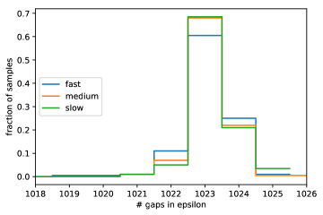
Figure 4: The fraction of samples having a given number of gaps in the interval ${\cal D}=[-\varepsilon,0]$. The size of the system is $N=1024$ and the simulations where performed on $200$ samples at $\alpha=5$ and $\sigma=0.22$. The peak is at the isostatic value $N-1$ and we see deviation from perfect isostaticity of about very few, order one, gaps.

In the main text we have underlined that as soon as one enters in the RSB-UNSAT (jammed) phase of the linear perceptron, the gap distribution contains a delta peak for marginally satisfied gaps. In order to detect them we consider the smoothed cost function defined in Eq. (3) of the main text and we track the gaps that are contained within the interval ${\cal D}=[-\varepsilon,0]$ when annealing the smoothing parameter $\varepsilon$. In Fig. 4 we plot the fraction of samples versus the total number of gaps contained in the interval ${\cal D}$ for $N=1024$ for three different annealing protocols in epsilon:

• fast: rapid quench where $\varepsilon$ takes two values $\varepsilon=10^{-4},10^{-6}$.

• medium: quench where $\varepsilon$ takes progressively the following values $\varepsilon=10^{-2},10^{-3},10^{-4},10^{-5},10^{-6}$

• slow: $\varepsilon$ takes progressively the following values
  $\varepsilon=10^{-2},10^{-3},5\cdot 10^{-4},10^{-4},5\cdot 10^{-5},10^{-5},7\cdot 10^{-6},4\cdot 10^{-6},2\cdot 10^{-6},10^{-6}$

We clearly see a peak at the perfect isostatic value which is $N-1$ (note that the total number of degrees of freedom is $N-1$ because of the spherical constraint on $\underline{w}$). Essentially we find that the majority of the samples have exactly $N-1$ gaps in $[-\varepsilon,0]$ which means that they become marginally satisfied for $\varepsilon\rightarrow 0^{+}$. A small number of samples is off from isostaticity for just very few (order one) contacts as it happens at jamming (see for example Sec. II.C of the supplementary information of Charbonneau et al. (2015)). Therefore we qualitatively see that fluctuations away from perfect isostaticity are anomalously small as it happens at jamming Hexner et al. (2019).

References

- Liu and Nagel (2010) A. J. Liu and S. R. Nagel, Annu. Rev. Condens. Matter Phys. 1, 347 (2010).
- Tkachenko and Witten (1999) A. V. Tkachenko and T. A. Witten, Phys. Rev. E 60, 687 (1999).
- Wyart (2012) M. Wyart, Phys. Rev. Lett. 109, 125502 (2012).
- Lerner et al. (2013) E. Lerner, G. During, and M. Wyart, Soft Matter 9, 8252 (2013).
- Mueller and Wyart (2015) M. Mueller and M. Wyart, Ann. Rev. Cond. Matt. Phys. 6, null (2015).
- Charbonneau et al. (2015) P. Charbonneau, E. I. Corwin, G. Parisi, and F. Zamponi, Phys. Rev. Lett. 114, 125504 (2015).
- Charbonneau et al. (2014a) P. Charbonneau, J. Kurchan, G. Parisi, P. Urbani, and F. Zamponi, Nature Communications 5, 3725 (2014a).
- Charbonneau et al. (2014b) P. Charbonneau, J. Kurchan, G. Parisi, P. Urbani, and F. Zamponi, JSTAT 2014, P10009 (2014b).
- Kurchan et al. (2013) J. Kurchan, G. Parisi, P. Urbani, and F. Zamponi, J. Phys. Chem. B 117, 12979 (2013).
- Mézard et al. (1987) M. Mézard, G. Parisi, and M. A. Virasoro, Spin glass theory and beyond (World Scientific, Singapore, 1987).
- Biroli and Urbani (2016) G. Biroli and P. Urbani, Nature Physics 12, 1130 (2016).
- Franz and Spigler (2017) S. Franz and S. Spigler, Physical Review E 95, 022139 (2017).
- Jin et al. (2018) Y. Jin, P. Urbani, F. Zamponi, and H. Yoshino, Science advances 4, eaat6387 (2018).
- Jin and Yoshino (2017) Y. Jin and H. Yoshino, Nature communications 8, 14935 (2017).
- Rainone et al. (2015) C. Rainone, P. Urbani, H. Yoshino, and F. Zamponi, Physical Review Letters 114, 015701 (2015).
- Franz and Parisi (2016) S. Franz and G. Parisi, Journal of Physics A: Mathematical and Theoretical 49, 145001 (2016).
- Franz et al. (2015) S. Franz, G. Parisi, P. Urbani, and F. Zamponi, Proceedings of the National Academy of Sciences 112, 14539 (2015).
- Franz et al. (2017) S. Franz, G. Parisi, M. Sevelev, P. Urbani, and F. Zamponi, SciPost Physics 2, 019 (2017).
- Moore and Mertens (2011) C. Moore and S. Mertens, The nature of computation (OUP Oxford, 2011).
- Engel and Van den Broeck (2001) A. Engel and C. Van den Broeck, Statistical mechanics of learning (Cambridge University Press, 2001).
- Franz et al. (2018) S. Franz, S. Hwang, and P. Urbani, arXiv preprint arXiv:1809.09945 (2018).
- Yoshino (2018) H. Yoshino, SciPost Physics 4, 040 (2018).
- Griniasty and Gutfreund (1991) M. Griniasty and H. Gutfreund, Journal of Physics A: Mathematical and General 24, 715 (1991).
- Györgyi (2001) G. Györgyi, Physics Reports 342, 263 (2001).
- Majer et al. (1993) P. Majer, A. Engel, and A. Zippelius, Journal of Physics A: Mathematical and General 26, 7405 (1993).
- Györgyi and Reimann (1997) G. Györgyi and P. Reimann, Physical review letters 79, 2746 (1997).
- Györgyi and Reimann (2000) G. Györgyi and P. Reimann, Journal of Statistical Physics 101, 679 (2000).
- Zhu et al. (2004) J. Zhu, S. Rosset, R. Tibshirani, and T. J. Hastie, in Advances in neural information processing systems (2004) pp. 49–56.
- De Almeida and Thouless (1978) J. De Almeida and D. J. Thouless, Journal of Physics A: Mathematical and General 11, 983 (1978).
- Fletcher (2013) R. Fletcher, Practical methods of optimization (John Wiley & Sons, 2013).
- Jones et al. (01 ) E. Jones, T. Oliphant, P. Peterson, et al., “SciPy: Open source scientific tools for Python,” (2001–), [Online; http://www.scipy.org/].
- Note (1) The virtual forces can be obtained as the negative gaps in rescaled by for .
- Gardner (1988) E. Gardner, Journal of physics A: Mathematical and general 21, 257 (1988).
- Sommers and Dupont (1984) H.-J. Sommers and W. Dupont, Journal of Physics C: Solid State Physics 17, 5785 (1984).
- Hexner et al. (2019) D. Hexner, P. Urbani, and F. Zamponi, arXiv preprint arXiv:1902.00630 (2019).