Hydrodynamical moving-mesh simulations of the tidal disruption of stars by supermassive black holes

Abstract

When a star approaches a black hole closely, it may be pulled apart by gravitational forces in a tidal disruption event (TDE). The flares produced by TDEs are unique tracers of otherwise quiescent supermassive black holes (SMBHs) located at the centre of most galaxies. In particular, the appearance of such flares and the subsequent decay of the light curve are both sensitive to whether the star is partially or totally destroyed by the tidal field. However, the physics of the disruption and the fall-back of the debris are still poorly understood. We are here modelling the hydrodynamical evolution of realistic stars as they approach a SMBH on parabolic orbits, using for the first time the moving-mesh code arepo, which is particularly well adapted to the problem through its combination of quasi-Lagrangian behaviour, low advection errors, and high accuracy typical of mesh-based techniques. We examine a suite of simulations with different impact parameters, allowing us to determine the critical distance at which the star is totally disrupted, the energy distribution and the fallback rate of the debris, as well as the hydrodynamical evolution of the stellar remnant in the case of a partial disruption. Interestingly, we find that the internal evolution of the remnant’s core is strongly influenced by persistent vortices excited in the tidal interaction. These should be sites of strong magnetic field amplification, and the associated mixing may profoundly alter the subsequent evolution of the tidally pruned star.

1 Introduction

Supermassive black holes (SMBHs) have been observed in the centre of most massive galaxies (e.g. Ferrarese & Ford 2005), and are believed to play a fundamental role in galaxy evolution (e.g. Di Matteo et al. 2005). Most notably, by accreting gas from their surroundings, these objects are capable of emitting enormous amounts of energy. Unfortunately, actively accreting black holes (or AGNs) represent only a small fraction of the entire supermassive black hole population, making it challenging to observe them through most of their life time.

Alternatively, because SMBHs are usually embedded within dense stellar clusters, the disruption of stars can provide material to power short periods of activity (Frank & Rees 1976). When a star passes too close to a black hole, the tidal forces overcome its self-gravity, which tears the star apart. A fraction of the stripped stellar material remains bound to the SMBH, eventually forming an accretion disc and powering activity that can last from months to years (Rees 1988), with peak values even comparable to the Eddington luminosity. These events are often referred to as tidal disruption events (TDEs), and they constitute a powerful indirect probe for studying black holes in the centre of galaxies, both in the local and distant Universe.

The theoretical basis to understand the emission from TDEs was laid down during the eighties in seminal works by Lacy et al. (1982), Rees (1988), Phinney (1989), and from a numerical perspective, Evans & Kochanek (1989). Their models showed that TDEs were detectable from UV to soft X-ray wavelengths with a light curve decreasing characteristically as $t^{-5/3}$. TDE candidates were later observed with properties in broad agreement with these theoretical predictions (e.g. Bade et al. 1996; Komossa & Bade 1999; Gezari et al. 2006; Komossa et al. 2008; van Velzen et al. 2011), strengthening this theoretical background. However, detailed observations of different TDE candidates have also found signatures that cannot be explained by the standard model (see the illustrative cases presented in Bloom et al. 2011; Gezari et al. 2012), suggesting that the picture is more complex than originally modelled.

The tidal disruption of a star and the subsequent fallback of gas is primarily governed by gravity, hence the basic principles of TDEs are well understood. However, in reality there are several additional physical processes at play, making the accurate analytical (or semi-analytical) modelling of these events quite challenging. Numerical hydrodynamical simulations are therefore the tool of choice for more detailed calculations. There has been significant progress on this front in recent years, helped also by the development of an increasing variety of suitable hydrodynamical codes. TDE simulations typically used either the Lagrangian smoothed particle hydrodynamics (SPH) technique (e.g. Lodato et al. 2009; Rosswog et al. 2009; Tejeda & Rosswog 2013; Coughlin & Nixon 2015; Bonnerot et al. 2016a; Coughlin et al. 2016; Sa̧dowski et al. 2016; Mainetti et al. 2017), or Eulerian grid-based methods (e.g. Evans & Kochanek 1989; Khokhlov et al. 1993a, b; Frolov et al. 1994; Diener et al. 1997; Guillochon et al. 2009; Guillochon & Ramirez-Ruiz 2013; Cheng & Bogdanović 2014). Although both of these approaches have their particular advantages, they also have some important limitations. Grid-based codes, for example, are not manifestly Galilean invariant and do not conserve angular momentum, which is crucial to accurately follow orbits. On the other hand, SPH methods tend to significantly broaden shocks, are associated with numerical surface tension effects which suppress mixing, and are comparatively noisy. These numerical deficits could introduce significant inaccuracies in simulations of TDEs, either during the disruption itself, the subsequent fallback of stripped material, or the hydrodynamical evolution of a partially disrupted star.

In recent years, new simulation methods have been developed with the goal of combining the advantages of both SPH and grid-based techniques while avoiding some of their disadvantages. In particular, new quasi-Lagrangian algorithms where the volume is discretised using a set of mesh-generating tracers that move with the fluid, as pioneered in the hydrodynamical code arepo (Springel 2010), have proven to be a robust and versatile tool to model a large variety of astrophysical systems (e.g. Greif et al. 2011; Vogelsberger et al. 2012; Nelson et al. 2013; Marinacci et al. 2014; Zhu et al. 2015; Ohlmann et al. 2016; Weinberger et al. 2017; Springel et al. 2018). In particular, because the mesh moves with the gas, highly supersonic flows do not suffer accuracy degradation due to advection errors in this approach, while the good shock-capturing accuracy and the ability to follow turbulence of ordinary mesh-based techniques are retained. These features are ideal for the TDE problem.

In this paper, we present a suite of simulations of the disruption of zero-age-main-sequence stars by a SMBH, from the first approach until several hours after periapsis, using arepo. Our models for the first time apply the moving-mesh technique to TDEs, and also represent the first examples of this type of simulations based on realistic stellar structure profiles. Previously, the structure of main sequence stars in tidal disruption simulations has been modelled almost exclusively using single polytropes. While this can be a decent approximation in many cases, it does not allow for more evolved stars that tend to be more centrally concentrated.

The paper is organised as follows. We describe the numerical methods and setup of our models in Section 2. In Section 3, we present a determination of the critical distance at which the star is completely destroyed, and the corresponding energy distribution and fallback rate of the debris. In Section 4, we study the evolution of the surviving stellar core after a partial disruption. We finally summarise and discuss our results in Section 5.

2 Numerical methods

We simulate the close encounter between a star and a single black hole using the finite volume hydrodynamics code arepo (Springel 2010; Pakmor et al. 2016). This code solves the Euler equations using a finite-volume approach on an unstructured Voronoi mesh that is generated from a set of points that move with the flow. The mesh admits the application of second-order accurate Godunov methods for evolving the fluid state in time, similar to the ones known from standard Eulerian finite volume hydrodynamical codes. However, the fluxes across cell boundaries are solved in the moving frame of mesh faces, which have minimal residual motion with respect to the fluid itself. This greatly diminishes advection errors inherent in ordinary Eulerian treatments, and prevents that the arepo results degrade in their accuracy with increasing bulk velocity of the star. At the same time, the use of a second-order accurate reconstruction yields high spatial and temporal accuracy, yielding a considerably faster convergence rate than achieved in SPH, where numerical noise and errors in discrete kernel sums cause much slower convergence speeds. Also, our method does not need to impose an artificial viscosity and naturally resolves mixing that may happen in a multidimensional flow.

Another advantage of the quasi-Lagrangian nature of arepo lies in its automatic adaptivity to the flow, allowing the spatial resolution to smoothly and continuously adjust to the mass density without imposing preferred grid directions. The full spatial and temporal adaptivity of the scheme is further strengthened by the ability to refine or derefine cells as needed, similar to how this is done in adaptive mesh refinement codes. We use these features to maintain constant mass resolution within the star and its stripped material, while guaranteeing a minimum spatial resolution in low density regions throughout the computational domain. Taken together, we think this method is hence particularly well suited for the TDE problem.

Figure 1: Density profiles of a $1\,{\rm M}_{\odot}$ ZAMS star. The light blue solid line shows the one dimensional profile from MESA, while the orange points display the individual densities computed by arepo after the relaxation run. For clarity the latter is shown only for a subset of 2000 randomly selected gas cells. For comparison, the green dashed line shows a polytropic profile with index $\gamma=4/3$, and the same total mass and radius of the 1D profile. This polytropic profile is often used to represent high-mass stars.

The stellar model we use in our tidal disruption simulations is created with the help of the stellar evolution code MESA (Modules for Experiments in Stellar Astrophysics; Paxton et al. 2011; Paxton et al. 2013), version 7623. We create a zero-age main sequence (ZAMS) star of mass $1\,{\rm M}_{\odot}$ and metallicity 0.02 as an input model for the hydrodynamics simulations.

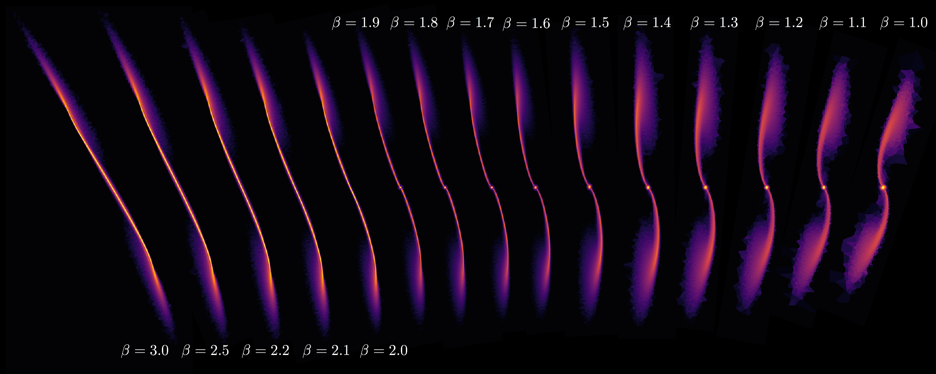
Figure 2: Total column density (in logarithmic scale) of each simulation’s final output for the disruption of a $1\,{\rm M}_{\odot}$ ZAMS star by a $10^{6}\,{\rm M}_{\odot}$ black hole. Each output is obtained $1.5\times 10^{5}$ seconds after periapsis, and is labelled with the corresponding value of the penetration parameter $\beta$, with the deepest encounter starting from the left. Here we observe the transition from the regime where the star is completely destroyed for deep encounters ($\beta\gtrsim 2$), to a small surviving core for smaller penetration parameters.

To produce the actual three-dimensional initial distribution of gas cells we follow a procedure fully described in Ohlmann et al. (2017) that we briefly summarise here. First, the one-dimensional stellar profile from MESA is mapped to a 3D grid using concentric shells with a HEALPix angular distribution on each shell. We place this spherical distribution into a small periodic box with $4\,R_{\odot}$ on a side and a very low background density of $10^{-16}$ g cm^-3. This configuration is then relaxed using a damping procedure over a time $10\,t_{\rm dyn}$, where $t_{\rm dyn}$ is the sound crossing time of the star. This is done to eliminate spurious velocities resulting from the discretization on our mesh, and results in a stable profile according to the stability criteria defined in Ohlmann et al. (2017).

We show the resulting stellar density profile in Fig. 1. The light blue solid line is the spherically symmetric profile from MESA, while the orange points correspond to the individual densities computed by arepo at the end of the relaxation run. We treat the gas as ideal, with an adiabatic equation of state and an adiabatic index of $5/3$. Note that the stellar profile after relaxation follows very closely the initial MESA profile at most radii, with the exception of the stellar surface where the initial density profile drops to sharply. This discrepancy arises because a significantly larger number of cells would be necessary to more accurately resolve the steep gradient at the stellar surface. As this region contains a negligible fraction of the total stellar mass, this is not necessary in our application and this disagreement does not affect our results.

We additionally show a polytropic profile with index $\gamma=4/3$ in Fig. 1 (green dashed line), which is often used to represent high-mass stars in this type of simulations. This profile is not dramatically different from the one obtained from MESA, only slightly more centrally concentrated, and arguably not a bad approximation for our star. However, the strength of the procedure presented in this paper is that it can be extended to any stage of stellar evolution, which opens up the possibility of modelling tidal disruptions for a whole suite of different stars, with varying mass and age, but always using a realistic internal structure. This includes giant stars, for example, where the core could additionally be replaced by a point mass to represent the extreme density contrast between the core and the envelope (Ohlmann et al. 2017) in an efficient fashion. As demonstrated by Guillochon & Ramirez-Ruiz (2013), the stellar structure is crucial for determining the characteristics of the disruption (e.g. the critical distance for total disruption and the energy distribution of the debris). Consequently, it is of paramount importance to use a physically motivated structure for the stars in TDE simulations to ultimately produce realistic light curve predictions.

Once we have the relaxed stellar profile, we can proceed to model the star’s tidal disruption by the black hole. In our simulations, the SMBH is simply modelled as an external Newtonian point potential, located at the centre of the domain, with a total mass of $M_{\rm BH}=10^{6}\,{\rm M}_{\odot}$. One of the most relevant scales to take into account when modelling TDEs is the distance at which the tidal forces of the black hole are larger than the star’s gravity at its surface, which is referred to as the tidal radius

$$r_{t}\equiv R_{*}\quantity(\frac{M_{\rm BH}}{M_{*}})^{1/3}\simeq 7\times 10^{12}\,\mbox{cm}\,\quantity(\frac{M_{\rm BH}}{10^{6}M_{\odot}})\quantity(\frac{R_{*}}{R_{\odot}})\quantity(\frac{M_{*}}{M_{\odot}})^{-1/3},$$ (1)

where $R_{*}$ and $M_{*}$ denote the radius and mass of the star, respectively, and $M_{\rm BH}$ is the mass of the black hole. Inside this sphere the star’s gravity can no longer prevent material from being stripped, and the star is disrupted at least partially. With our choice of black hole mass, the black hole to stellar mass ratio corresponds to $q=10^{-6}$, which results in a tidal radius of $r_{t}=100\,R_{*}$.

The Newtonian approximation for the black hole is still reasonable for our models, since we are simulating encounters were the closest approach is $\sim 15\,r_{g}$, where $r_{g}=GM_{\rm BH}/c^{2}$ is the gravitational radius of the black hole. The relativistic corrections during periapsis in this regime are expected to be small (Cheng & Bogdanović 2014; Stone et al. 2019). A more accurate treatment is needed during the fallback and accretion of the debris, since relativistic effects are important for the formation of the accretion disc and its evolution (see e.g. Bonnerot et al. 2016a). This process, however, is beyond the scope of the present work as we focus on the disruption process itself.

To model the disruption, we place the relaxed star in a periodic box with a side length of $2.1\times 10^{15}\,{\rm cm}$ (equivalent to $300\,r_{t}$), with a low background density of $10^{-16}\,{\rm g\,cm}^{-3}$. All the simulations presented in this paper were stopped after about 44 hours, with the leading arm of the disrupted star still being far from the boundary, ensuring that there is no stellar mass flowing over an edge of the domain and reappearing from the opposite side. Consequently, we do not have unphysical effects due to the finite size of the box. We note that in contrast to the hydrodynamics, the gravity of the BH and the self-gravity of the stellar material are treated without periodic boundary conditions.

The initial velocity of the star is set up such that the star’s centre of mass describes a parabolic orbit, with the location of the periapsis radius given by

$$r_{\rm p}=\frac{r_{\rm t}}{\beta},$$ (2)

where $\beta$ is the so-called “penetration” parameter. We vary this parameter to obtain a suite of simulations with different stellar orbits. In this paper, we present the results of 15 simulations, with $\beta$ between 1 and 3. In each case, the star was placed at an initial distance from the black hole equivalent to $5\,r_{t}$, which ensures that the star’s stability is preserved at the beginning of the approach. With this choice of parameters, the periapsis of the star occurs between about 2 and 3 hours from the start of the simulation, depending on the impact parameter.

Because we want the star to be represented by at least a total of roughly $2\times 10^{5}$ cells, we set the refinement cell criterion to a target cell mass of $M_{\rm target}=9.8\times 10^{27}\,{\rm g}=4.9\times 10^{-6}\,{\rm M}_{\odot}$. In addition to the mass refinement criteria, we use a volume limit criterion in which neighbouring cells are refined such that the ratio of their volumes is never larger than 5. This allows us to have more resolution elements in regions where there is little mass, namely, in the outer layers of the star, and later on, in the streams of stripped gas. At the start of the simulations we have a total of about $2.3\times 10^{5}$ cells, with $3\times 10^{4}$ forming part of background grid, and a mean cell mass of $8.9\times 10^{27}\,{\rm g}$. By the end of the runs, the total number of cells has increased to about $2.4\times 10^{5}$ with a mean cell mass of $8.5\times 10^{27}\,{\rm g}$, thanks to the mesh refinement. To confirm the convergence of our results, we have also run a subset of models with 10 times the resolution of our standard setup, finding no appreciable difference. We thus only show the simulations with the standard resolution explained above.

3 Influence of the penetration parameter

3.1 The limit between total and partial disruption

As explained in the previous section, we simulate stellar orbits with pericentre distances always smaller or equal to the tidal radius. Contrary to intuition, however, this does not mean that the star will be completely destroyed in each of the simulated encounters, since the definition of $r_{t}$ only considers the stellar gravity on its surface. Whether the star is completely or partially destroyed for a given impact parameter depends almost exclusively on the internal stellar structure, with the more centrally concentrated stars being able to survive deeper encounters (e.g. Guillochon & Ramirez-Ruiz 2013).

In Figure 2, we show density maps of our simulations. Each output is obtained $1.5\times 10^{5}$ seconds after periapsis, which corresponds to approximately 50 dynamical times. In this figure, we can observe the transition between total disruption for the deepest encounters, to the point where the core starts re-collapsing for lower values of $\beta$. Motivated by this result, we seek to identify the critical distance of the star to the SMBH at which the encounter results in a total disruption.

Since we do not simulate the encounter long enough for the core to completely re-collapse, we compute the total stellar mass loss $\Delta M$ at the end of our simulations by using the method introduced by Guillochon & Ramirez-Ruiz (2013), in which the gas gravitationally bound to the star is iteratively determined. The specific binding energy of each cell is computed as

$$E_{*,i}=\frac{1}{2}(\mathbf{v}_{i}-\mathbf{v}_{*})^{2}+\phi_{i},$$ (3)

where $\mathbf{v}_{i}$ is the cell’s velocity, and $\phi_{i}$ is the gravitational potential exerted by the rest of the gas onto each cell, which is computed directly by arepo through its gravity solver. The star’s velocity $\mathbf{v}_{*}$ is initially chosen to be equal to the velocity of the highest density peak. After the first estimation of $E_{*,i}$, we then consider only cells with $E_{*,i}<0$ to find a more robust value for the star’s location and velocity

$$\mathbf{r}_{*}=\frac{\sum_{E_{*,i}<0}m_{i}\mathbf{r}_{i}}{\sum_{E_{*,i}<0}m_{i}},$$ (4)

$$\mathbf{v}_{*}=\frac{\sum_{E_{*,i}<0}m_{i}\mathbf{v}_{i}}{\sum_{E_{*,i}<0}m_{i}}.$$ (5)

We iterate this procedure until the star’s velocity has converged to a constant value. Subsequently, the stellar mass loss is simply taken as all the gas cells that are unbound from the star, i.e., which have $E_{*,i}>0$.

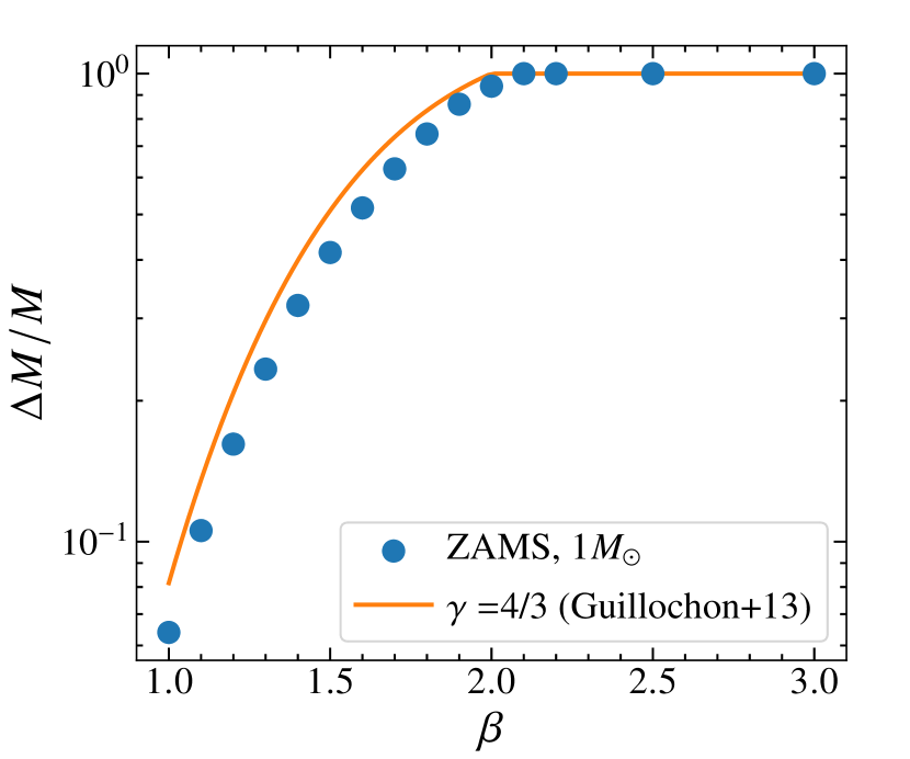
Figure 3: Total mass that is tidally stripped from the star, in units of the initial mass, as a function of the penetration parameter. This quantity is measured at the end of the simulations. When this value reaches unity, full disruption has occurred. The solid line shows the fitting formula obtained by Guillochon & Ramirez-Ruiz (2013) for a $\gamma=4/3$ polytrope.

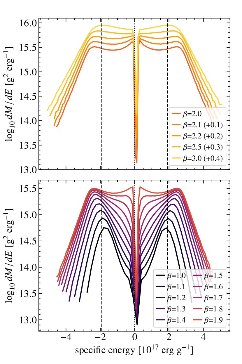
Figure 4: Distribution of specific binding energy of the stripped material for different penetration parameters, increasing from the darkest to the lightest line colour. The vertical dashed lines indicate the expected energy spread from the ‘frozen in’ approximation. This stripped material corresponds to the value of the total mass unbound from the star, as presented in Fig. 3, measured at the end of the simulation. For clarity we separate the cases in which there is a surviving core ($\beta<2$, lower panel) and of total disruption ($\beta\geq 2$, upper panel). Furthermore, in the upper panel all the cases are arbitrarily shifted upwards with respect to $\beta=2$, and the relative shift is indicated in the legend.

In Fig. 3, we show the total mass loss as a function of the penetration parameter. Because $\Delta M$ is expressed in terms of the star’s initial mass, a total disruption occurs when this value reaches unity. We check the convergence of $\Delta M$ through the quantity

$$\mathcal{F}(t)\equiv\absolutevalue{\frac{\dot{M}_{\rm bound}}{M_{\rm bound}}}(t-t_{p}),$$ (6)

where $M_{\rm bound}$ is the total mass still bound to the star and $t_{p}$ is the time of periapsis (Guillochon & Ramirez-Ruiz 2013). We find the two expected regimes: small and decreasing values of $\mathcal{F}$ when the core survives, whereas $\mathcal{F}\sim 1$ at all times for total disruptions. Notice that $M_{\rm bound}$ never formally reaches zero since the tidal forces vanish towards the very center of the stellar remnant, and thus this procedure always yields some gravitationally bound material, even if the star is completely destroyed. Nevertheless, following a total disruption, the bound gas quickly changes with time as the material is perpetually stretched to never re-collapse, resulting in $\mathcal{F}\sim 1$ at all times.

In Fig. 3, we also show the fitting formula obtained by Guillochon & Ramirez-Ruiz (2013) for the disruption of a $1\,{\rm M}_{\odot}$ star, represented with a $\gamma=4/3$ polytrope. As discussed in the previous section, this profile has a similar shape as our ZAMS star, but is more centrally concentrated. As a consequence, the mass loss as a function of $\beta$ in our simulations is quite similar to the one obtained with a polytrope, including the value of the critical distance for total disruption. The star in our simulations looses slightly less mass with respect to the polytrope, which is most likely a consequence of the different concentrations, because our star has less mass than the corresponding polytrope at a given radius in the inner regions.

Another effect that might cause different mass loss as a function of impact parameter is the numerical technique. Mainetti et al. (2017) numerically modelled the disruption of stars (represented by polytropes) using different simulation techniques: mesh-free finite mass, traditional SPH, and “modern” SPH. They find that the critical distance depends weakly on the method. Considering that the moving-mesh approach of arepo represents a different technique with respect to the ones tested in Mainetti et al. (2017), one expects some differences to our results as well, although they are probably subdominant with respect to the differences in the actual stellar structure between our ZAMS star and a polytrope.

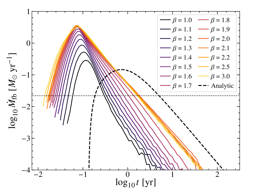
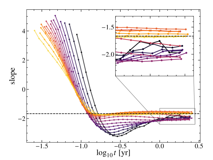
Figure 5: Upper panel: Fallback rates onto the SMBH as a function of time for the different orbits modelled. As indicated in the legend, the penetration parameter increases from darker to lighter lines. The black dashed line shows the rate computed assuming that the energy distribution is frozen in at the tidal radius, while the dotted horizontal line corresponds to the Eddington mass accretion rate for a $10^{6}\,{\rm M}_{\odot}$ SMBH. Lower panel: Time evolution of the logarithmic derivative of each fallback rate presented in the upper panel. The dashed horizontal line indicates the theoretical value of -5/3.

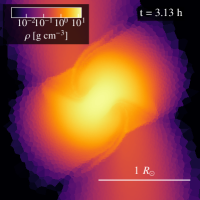
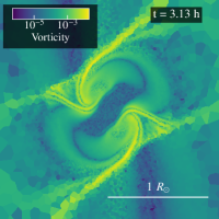
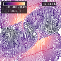
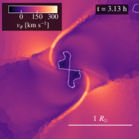
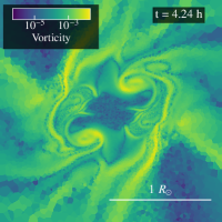
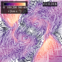
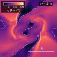
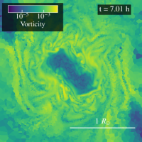
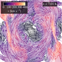
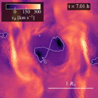
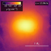
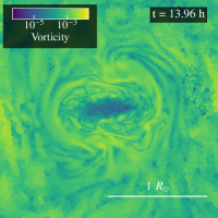
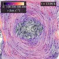
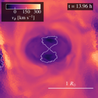
Figure 6: Time evolution of the surviving stellar core after a grazing encounter ($\beta=1.6$) with a SMBH. From left to right, we show 2D slices of density, vorticity, total velocity and azimuthal velocity. All plots are centred on the core’s centre of mass with a box side of $2\,R_{\odot}$, and the time label is such that $t=0$ corresponds to periapsis. The dashed lines in the right-hand column mark the point where the azimuthal velocity is zero.

3.2 Energy distribution and fallback rate

As shown by Rees (1988), during the disruption of a star on a parabolic orbit roughly half of the material stripped from the star is bound to the black hole. This gas will then fallback to the black hole, powering a short period of activity. The fallback rate of this material as a function of time can be obtained using Kepler’s third law,

$$\dot{M}(t)=\derivative{M}{E}\derivative{E}{t}=\frac{(2\pi GM_{\rm BH})^{2/3}}{3}\derivative{M}{E}t^{-5/3}.$$ (7)

The characteristic $t^{-5/3}$-decay expected from these type of events (see e.g. Komossa 2015) is thus intimately related to the distribution of specific binding energy ($\differential{M}/\differential{E}$).

As we presented in the previous section, we have an estimation of the total mass lost by the star, measured at the end of our simulations. We show the distribution of binding energy of this stripped material for all impact parameters in Fig. 4. The dashed lines in this figure show the expected spread in binding energy if the distribution was ‘frozen in’ at the tidal radius. This approximation is based on the consideration that inside the tidal radius only the black hole gravity determines the energy distribution, and the internal forces of the star are negligible. Using this approximation, the energy spread can be obtained by Taylor-expanding the black hole gravitational potential across the star, yielding

$$\Delta E=\frac{GM_{\rm BH}}{r_{t}^{2}}R_{*}.$$ (8)

The spread observed in our simulations is noticeably larger than this estimate. This occurs because, once the star enters the tidal radius, forces inside the star re-distribute some of the energy, and the final distribution is no longer determined solely by the black hole gravity. For instance, Lodato et al. (2009) found that shocks in the gas after the disruption promote the appearance of wings in the tails of the energy distribution. Alternatively, Coughlin et al. (2016) argue that these deviations result from the combination of the star’s self-gravity and the in-plane compression happening near periapsis.

Using equation (7) we can map the distribution of binding energy to the fallback rate of gas onto the black hole, which is shown in Fig. 5 for every impact parameter. It is important to stress that this fallback rate does not translate directly to an accretion rate onto the black hole, since the gas would likely first settle into an accretion disc, where the dissipation of energy and angular momentum occurs on a viscous timescale.

Under the ‘frozen in’ approximation, the energy distribution is completely determined by the fraction of stellar mass at each slice pointing towards the black hole. We now use the formalism presented by Lodato et al. (2009) to compute the energy distribution and corresponding fallback rate, which can be expressed as

$$\derivative{M}{x}=2\pi\int_{0}^{H_{x}}\rho_{*}h\differential{h},$$ (9)

where $x$ is the radial coordinate inside the star, $H_{x}=\sqrt{R_{*}^{2}-x^{2}}$ is the radius of each slice, and $\rho_{*}$ is the one-dimensional density profile generated by MESA. Because the latter is not an analytical profile, we numerically integrate equation (9) to obtain the black dashed line in Fig. 5. Despite the crudeness of assuming that the energy distribution is frozen in at the tidal radius, it is still frequently being used as an approximation to compute fallback rates coming from the stellar disruption (e.g. Gallegos-Garcia et al. 2018), yet the accuracy of this approach is quite limited based on our results.

In the lower panel of Fig. 5 we show the time evolution of the logarithmic derivative of the fallback rates, i.e. the slope. From the inset in this plot it is clear that for the encounters that result in a partial disruption ($\beta\lesssim$1.8) the slope approaches steeper values than the theoretical expectation at late times. As explained by Guillochon & Ramirez-Ruiz (2013), this is due to the gravitational influence of the surviving core, countering the black hole’s tidal force for the closest gas. This influence monotonically depletes gas at lower energies after the peak (see Fig. 4, lower panel), which is the material that determines the asymptotic value of the fallback rate. On the other hand, we find that the cases $\beta=1.9,2.0,2.1,2.2$ present shallower slopes compared to $-5/3$. This behaviour is also found by Guillochon & Ramirez-Ruiz (2013), and comes from the fact that in the borderline cases where the star is barely completely destroyed, some of the core material slowly shrinks as it is pulled apart. Consequently, and in contrast with more grazing encounters, these cases present an increase of gas towards lower energies (see Fig. 4, upper panel).

For deeper encounters ($\beta\gtrsim 2.5$), the star is quickly destroyed at pericentre, and thus the slope is consistent with $-5/3$. This occurs because the energy distributions do flatten at low energies. However, it is important to clarify that the large dip observed around $E=0$ is the result of our iterative procedure to determine the stripped mass. As previously discussed, because the tidal forces vanish towards the debris’ centre of mass, this procedure always yields a non-zero amount of self-bound gas, which is thus excluded from the determination of the energy distribution. However, this affects only material with fallback timescales of over a decade, and does not change the rates shown in Fig. 5. In any case, because $\mathcal{F}\sim 1$ at all times for total disruptions (see equation 6), the gas considered as self-bound by this method would eventually become negligible if we were to run the simulation for a long enough time.

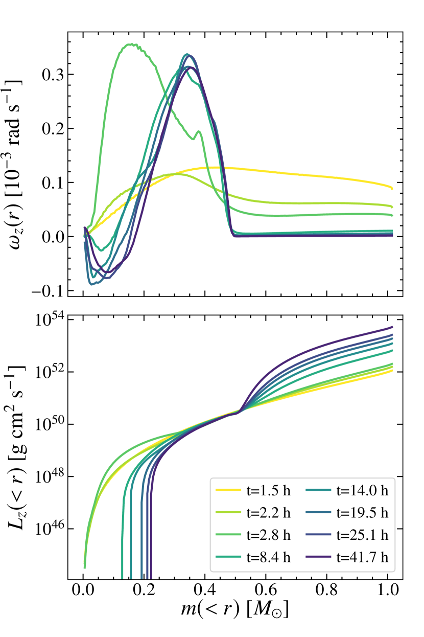
Figure 7: Upper panel: Time evolution of the surviving core’s angular frequency during the interaction. Lower panel: Time evolution of the star’s angular momentum profile. In both panels, time goes from lighter to darker lines. Notice that we have replaced the radial coordinate by the enclosed mass, since the extent of the gas changes dramatically during the interaction.

4 Hydrodynamics of the surviving core

As the star approaches the black hole, it is stretched into a prolate spheroid along the direction of motion. Once the stars reaches periapsis, its leading edge is slightly closer to the SMBH, where the tidal forces produce a torque on the whole star, effectively inducing some level of rotation (see e.g. Guillochon et al. 2009). Consequently, following a partial disruption, the surviving stellar core rotates as it breaks away from the black hole. The complex fluid motions produced during these later stages can be studied with high accuracy using arepo, thanks to its quasi-Lagrangian nature and high hydrodynamical accuracy compared to particle-based techniques.

To study the hydrodynamical evolution of the surviving core after a grazing encounter we choose $\beta=1.6$ as a representative case. In this example, roughly half of the star’s mass remains bound to the core (see Fig. 3), although most of our conclusions apply also to other instances where the stellar core survives. The early evolution of the star after periapsis is shown in Fig. 6 with slices in the $x-y$ plane. The density slices (left column) show the material as it is being stripped from the star, with some of the bound material forming a diffuse halo around the core. To capture the complexity of the motions, we analyse the vorticity of the fluid, defined as

$$w=\norm{\curl{\mathbf{v}}}.$$ (10)

We show slices of this quantity inside the star in the second column of Fig. 6. In contrast to the density field, the vorticity of the fluid shows plenty of substructure within the surviving core, mainly in the form of small filaments. This points to a turbulent evolution of the star after the encounter. Furthermore, the substructures observed seem to indicate that the material inside the core is stirred up by this turbulence, probably inducing significant mixing in the gas.

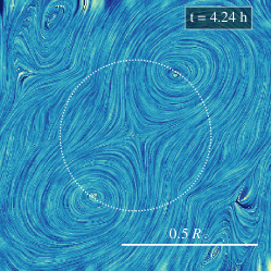
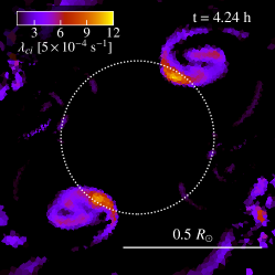
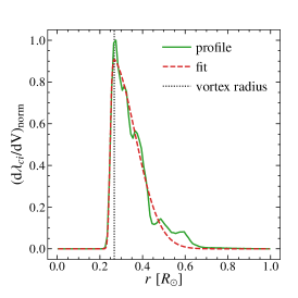
Figure 8: Example of the prominent vortices developed inside the surviving core. The left-hand panel shows the morphology of the velocity field inside the core using the line integral convolution method, while the center panel displays a slice of the “swirling strength” $\lambda_{ci}$ of the same gas. The right-hand panel shows the density profile of $\lambda_{ci}$ (normalized to the maximum value), where the peak indicates the radial position of the vortex pair, as shown in each panel with a dotted line.

These complex motions are induced by the differences in velocity with respect to the material surrounding the star and the gas that is being stripped, which can be observed in the two right columns of Fig. 6. The total velocity in the reference frame of the star (middle right column), displayed with stream lines, clearly shows the presence of two prominent vortices on opposite sides of the core, formed as part of the re-accretion of some initially stripped material. This vortex pair rotates with the surviving core, although the gas trapped inside has much lower azimuthal velocity (Fig. 6, right column) than the rest of the surrounding gas, in fact even reaching negative (counterrotating) values. Hence the star is constantly being stirred up by these movements, driving the turbulent behaviour. We note that the vortices are still present by the end of our simulation, roughly after 50 stellar dynamical times, which shows the high persistence of this structure.

Motivated by these complex motions, we study the evolution of the stellar rotation during the interaction. Since the star’s movement occurs in the $x-y$ plane, the relevant axis is the $z$-direction, hence we focus our attention only on this component, unless stated otherwise. Based on the azimuthal velocity of the gas shown in the right column of Fig. 6, we do not expect the star to behave as a solid body, hence we divide it into shells where we compute different diagnostic quantities. For a rigid body, the angular frequency and the total angular momentum are related by $L_{z}=I_{z}\omega_{z}$, with $I_{z}$ being the moment of inertia with respect to the $z$-axis. Thus, for each shell we can estimate the average angular frequency as

$$\langle\omega_{z}\rangle(r)=\frac{L_{z}}{I_{z}},$$ (11)

with

$$I_{z}(r)=\sum_{i}m_{i}r_{\perp,i}^{2},$$ (12)

and

$$L_{z}(r)=\sum_{i}m_{i}r_{\perp,i}v_{\phi,i},$$ (13)

where $r_{\perp,i}$ is the perpendicular distance to the star’s rotation axis, and $v_{\phi,i}$ is the azimuthal velocity. Notice that the summation goes over all cells inside each particular shell.

We show the star’s rotation during its interaction with the SMBH in Fig. 7. The top panel of this figure shows the evolution of the angular frequency profile, while the bottom panel gives the cumulative angular momentum profile. The angular frequency shows strong evolution, starting roughly with rigid-body rotation (yellow line). As the outer layers of the star are stripped, the core spins up, departing greatly from a rigid-body. Notice that for these profiles we have replaced the radial coordinate by the enclosed mass, because once the star is disrupted, the gas changes dramatically in extent. Recall that approximately half of the star survives for this impact parameter, hence $m(<r)\sim 0.5\,{\rm M}_{\odot}$ corresponds to the remnant’s outer edge.

Roughly one day after the encounter, the remains of the star approach an equilibrium where the outer layers rotate fast, while the inner core is counter-rotating. It is important to clarify, however, that this result does not imply that the inner core counter-rotates as a whole, but rather that its total angular momentum is negative. As can be seen in the right column of Fig. 6, the only material that has negative azimuthal velocity is inside the two vortices, and thus this result shows that these structures dominate the angular momentum budget. By analysing the angular momentum of the gas (Fig. 7, lower panel) it is clear that during this period there are no net torques acting at $m(<r)\sim 0.5\,{\rm M}_{\odot}$, since the total value remains roughly constant. Consequently, the evolution observed inside the core comes from the re-accommodation of the different layers, which in turn re-distributes the angular momentum.

4.1 Vortex identification

Due to the differential rotation inside the surviving core and with respect to the surrounding material, there are clear vortices induced in the fluid. In particular, about 2 hours after periapsis, two prominent and persistent vortices develop inside the star. These structures rotate together with the surviving core and clearly seem to have an impact on the dynamics of the innermost region of the remnant.

In order to directly relate the presence of these two vortices to the observed evolution, we need a method to identify their position in every output. Because the instantaneous stream line pattern of a fluid can be reconstructed through its velocity gradient, we can characterize the motions inside the star using the eigenvalues of the velocity gradient tensor $A$ (Chong et al. 1990). This tensor is defined as $A_{ij}=\partialderivative*{v_{i}}{x_{j}}$, and each gradient component is directly computed by arepo for each cell at every timestep during the hydrodynamical run (Pakmor et al. 2016). Following Chong et al. (1990), we expect the fluid to describe closed or spiralling orbits (such as the ones expected in vortices) if two of the eigenvalues of $A$ form a complex conjugate pair. We define a vortex core as the region where the velocity gradient tensor $A$ has complex eigenvalues.

As described by Chong et al. (1990), the characteristic equation for $A$ is given by

$$\lambda^{3}+\lambda^{2}P+Q\lambda+R=0,$$ (14)

where $P$, $Q$, and $R$ are the three invariants of $A$,

$$\begin{split}P&=-\tr(A),\\ Q&=\frac{1}{2}\quantity[\tr(A)^{2}-\tr(A^{2})],\\ R&=-\det(A).\end{split}$$ (15)

The discriminant of equation (14) can be written as

$$\Delta\equiv 27R^{2}+(4P^{3}-18PQ)R+(4Q^{3}-P^{2}Q^{2}).$$ (16)

The velocity gradient tensor will then have one real eigenvalue and a pair of conjugated complex eigenvalues whenever $\Delta>0$, and consequently we can use this condition to determine which cells belong to stream lines resembling vortices.

Additionally, to further characterise these vortices, we use the fact that the pair of complex eigenvalues can be written as $\lambda_{cr}\pm i\lambda_{ci}$, where $\lambda_{ci}$ is usually referred to as “swirling strength”, as it is a measure of the local swirling rate inside the vortex (Zhou et al. 1999; Chakraborty et al. 2005). Hence, for each gas cell satisfying the $\Delta>0$ condition, we use the imaginary part of its complex eigenvalues to quantify the strength of the spiralling motions inside the star. Finally, in order to capture vortices in approximately closed orbits, we consider gas cells that satisfy the conditions $\lambda_{ci}>\epsilon$ and $-\kappa\leq\lambda_{cr}/\lambda_{ci}\leq\delta$, where $\epsilon$, $\delta$, $\kappa$ take on non-negative values (Chakraborty et al. 2005). We find that $\epsilon=5\times 10^{-4}\,{\rm s}^{-1}$ and $\delta=\kappa=0.1$ are appropriate to capture the vortices observed in our simulations.

In Fig. 8 we show the motions in the stellar interior, 4 hours after periapsis, where a vortex pair is clearly present. The left-hand panel of this figure displays the stream lines of the fluid in the reference frame moving with the core. The centre panel shows $\lambda_{ci}$ of these cells. We can see clearly that the strength is higher for the gas inside the vortices, with the peak located on the rotation axis of both structures.

Finally, in order to estimate the position of the vortex pair in each output, we compute the radial profile of the swirling strength inside the star. An illustrative example is shown in the right-hand panel of Fig. 8. The profile displays the density of $\lambda_{ci}$, namely, for each spherical shell we sum $\lambda_{ci}$ of the contained cells and normalize by its total volume. We note that the presence of the vortex pair produces a very prominent asymmetric peak. However, since the fluid is highly turbulent within the surviving core, this profile can be rather noisy in some of the outputs, mainly due to the transient appearance of smaller vortices during the evolution. Consequently, we distinguish the main peak of each profile by fitting a skew-normal distribution, which can be expressed as

$$f(x)=\frac{c}{\sqrt{2\pi}}e^{-\frac{(x-a)^{2}}{2b^{2}}}\quantity[1+\erf\quantity(\frac{\alpha x}{\sqrt{2}})],$$ (17)

where $a$, $b$, $c$, and $\alpha$ are the fitting parameters, and $\alpha$ represents the “skewness” of the function. Note that for $\alpha=0$ this distribution is equivalent to a normal distribution. We find this function appropriate to approximate the asymmetric shape of the main peak, as seen in the example displayed in the right-hand side panel of Fig. 8 with the dashed red line. We assign the position of the vortex pair as the radius of the maximum value of the fitted function. The radial position of the vortex pair is shown with a dotted line on each panel of Fig. 8, and it is clear that this procedure yields a value that is consistent with the rotation axis of each vortex.

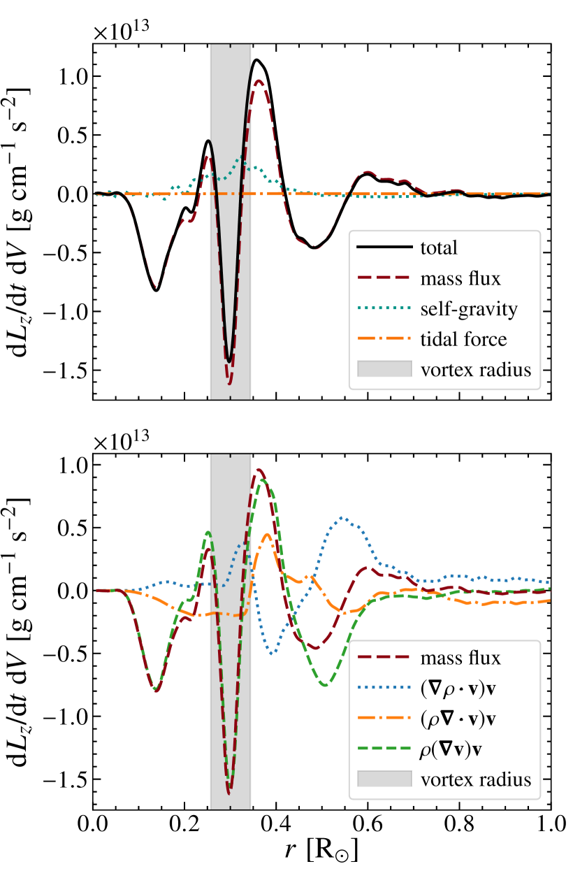
Figure 9: Azimuthally averaged torque profile inside the star, averaged over the time interval $t=3-25$ h. Upper panel: Individual contributions of the different terms to the total angular momentum evolution (solid line) as shown in equation (23): mass flux (dashed line), gas self-gravity (dotted line) and BH gravity (dotted-dashed line). Lower panel: Decomposition of the mass flux term of the upper panel as shown in equation (26).

4.2 Torque decomposition

As observed in Fig. 7, the rotation of the star evolves greatly after periapsis. In order to differentiate the forces responsible for this evolution, and to establish the possible role of the vortex pair, we compute the different torques inside the surviving core.

The total angular momentum of a spherical shell can be written as

$$\mathbf{L}_{\rm shell}=\int_{\rm shell}\mathbf{r}\crossproduct(\rho\mathbf{v})\differential V,$$ (18)

thus its time derivative is

$$\partialderivative{\mathbf{L}_{\rm shell}}{t}=\int_{\rm shell}\mathbf{r}\crossproduct\partialderivative{(\rho\mathbf{v})}{t}\differential V,$$ (19)

which gives us the total torque over the shell. From the Euler equation we have

$$\partialderivative{(\rho\mathbf{v})}{t}=-\divergence{}(\rho\mathbf{v}\mathbf{v}^{T})-\gradient P-\rho\gradient\phi,$$ (20)

which inserted into equation (19) gives us the different contributions to the momentum evolution of the shell.

Intuitively, one would expect the pressure term not to contribute to the total torque on each shell, since the pressure force points always radial over the spherical surfaces we are considering. To demonstrate that this is the case, we use the identity $\curl(P\mathbf{r})=P\curl\mathbf{r}+\gradient P\crossproduct\mathbf{r}$ to yield

$$\int_{\rm shell}\mathbf{r}\crossproduct\gradient P\differential V=-\int_{\rm shell}\curl(P\mathbf{r})\differential V.$$ (21)

Using the Green-Gauss theorem, we can transform the integral over the volume of the shell to one over the enclosing surface

$$\int_{\rm shell}\curl(P\mathbf{r})\differential V=\int_{\rm surface}P(\hat{\mathbf{n}}\crossproduct\mathbf{r})\differential S,$$ (22)

where $\hat{\mathbf{n}}$ is the outward pointing unit normal vector to the shell’s surface. Since by definition the normal vector to a spherical surface is radial (i.e., $\hat{\mathbf{n}}\equiv\hat{\mathbf{r}}$), the right-hand side of equation (22) vanishes, which is what we want to demonstrate.

Finally, we discretise equation (19) by summing over the cells enclosed by each shell, which gives us an estimate of the torque density profile

$$\frac{1}{\differential V}\derivative{\mathbf{L}_{\rm shell}}{t}=-\frac{1}{\Delta V}\sum_{i}\mathbf{r}_{i}\crossproduct\ \quantity[\divergence{}(\rho_{i}\mathbf{v}_{i}\mathbf{v}_{i}^{T})V_{i}+m_{i}\gradient\phi_{i}],$$ (23)

where

$$\Delta V=\sum_{i}V_{i}$$ (24)

is the total volume of the cells contained in the shell. The second term on the right-hand side of equation (23) is the torque coming from the forces acting on the gas, which in this case is only gravity. On the other hand, the first term can be interpreted as the specific angular momentum flux between the different shells.

The gravitational potential can be split into contributions from the gas self-gravity and the black hole potential. However, it is important to notice that the reference frame of the star is non-inertial, which in practice means that the gravitational force each gas parcel feels corresponds to a tidal stretching, which we can be expressed as

$$\gradient\phi_{\rm tidal}=\frac{GM_{\rm BH}}{r_{i}^{3}}\mathbf{r}_{i}-\frac{GM_{\rm BH}}{r_{*}^{3}}\mathbf{r}_{*}.$$ (25)

The top panel in Fig. 9 shows the different contributions to the torque per unit volume inside the surviving core. This radial profile is averaged over the time interval $t=3-25\,{\rm h}$ after periapsis. From this figure it is clear that the torque is completely dominated by the redistribution of mass inside the star, with a small contribution produced by the gas self-gravity. As expected, the black hole gravity is negligible at this stage, since the star is far from the tidal radius. The total torque has the largest (negative) value at $r\approx 0.3R_{\odot}$, which coincides with the position of the prominent vortex pair observed in our simulations.

The first term on the right-hand side of equation (20) can also be expanded to

$$\divergence{}(\rho\mathbf{v}\mathbf{v}^{T})=(\gradient\rho\dotproduct\mathbf{v})\mathbf{v}+(\rho\divergence\mathbf{v})\mathbf{v}+\rho(\gradient\mathbf{v})\mathbf{v}.$$ (26)

Notice that $(\gradient\mathbf{v})\mathbf{v}$ is a matrix vector multiplication, as $\gradient\mathbf{v}=\partialderivative*{v_{i}}{x_{j}}$ corresponds to the gradient velocity tensor. We show the contribution of the different terms from equation (26) in the lower panel of Fig. 9. We find that the dominant source of torque is the term given by the velocity gradient, mainly because the other two terms tend to cancel each other out. Since $\gradient\mathbf{v}$ is related to the vorticity of the fluid, this suggests that the vortex pair is responsible for the angular momentum transport inside the star, which results in the counter-rotating core observed in Fig. 7. To additionally support this mechanism, we can compare the amount of angular momentum transported from the inner core ($\tau_{\rm trans}$) with the value of the torque measured in our simulation ($\tau_{\rm vort}$). From Fig. 7 we have that initially the inner core has a total angular momentum of $\sim$ 10⁴⁹ g cm² s^-1, which is transported in the span of $\approx$20 h $\approx$ 7$\times$10⁴ s. This yields $\tau_{\rm trans}\sim$10⁴⁴ g cm² s^-2. On the other hand, from the torque density in Fig. 9 we obtain $\tau_{\rm vort}$$\sim$  10¹³ g cm^-1 s^-2 $\times$ $4\pi$ (0.3R_⊙)²  $\times$ 0.1R_⊙ $\sim$ 10⁴⁴ g cm² s^-2, where the total vortex volume corresponds to the shaded area in Fig. 9. Because these two torques are comparable, this estimation strengthens our conclusion that the vortices produce the evolution observed in the surviving core. We note that other examples of vortices responsible for angular momentum transport have been found in the context of hydrodynamical simulations of protoplanetary discs, where these spiralling motions are long-lived structures that drive compressive motions (e.g. Johnson & Gammie 2005).

We find that the vortices are quite persistent, being still present when we stop the simulations after several dynamical times of the core. This stability is expected given that the numerical viscosity is very low, and we are not including physical viscosity because non-perturbed stars can be approximated as inviscid given their extremely high Reynolds numbers (see Miesch & Toomre 2009, and references therein). However, for stellar cores that are the result of tidally disrupted stars this might not necessarily be the case, especially if there are strong magnetic fields. As shown by the numerical simulations of Guillochon & McCourt (2017) and Bonnerot et al. (2017), the vortex formation after the disruption significantly amplifies the magnetic field inside the surviving core, which can be a source of high viscosity. In fact, the vortices in their simulations disappear after a few dynamical times, indicating that the magnetic field is dissipating their energy. Consequently, in order to estimate a realistic dissipation timescale of the vortex pair formed within the core, the addition of magnetic fields is crucial.

5 Conclusions

In this paper, we have introduced a new suite of simulations to study the tidal disruption of stars by supermassive black holes, using for the first time the hydrodynamical moving-mesh code arepo. This code has been previously used to investigate a large number of astrophysical problems in the areas of cosmic structure formation and galaxy evolution, and it has also been used in a few selected applications in stellar astrophysics. We have here shown that it also provides a powerful tool to study TDEs with unprecedented accuracy. This is because arepo can accurately follow high-speed orbits while still well resolving mixing and shocks in the rest-frame of the moving fluid. This combination is usually not readily available with more standard numerical techniques, because SPH is comparatively noisy whereas Eulerian grid-based codes are diffusive for the high bulk velocities occurring in the TDE problem.

Since the appearance of flares produced by TDEs in the core of galaxies depends critically on whether the star is fully or partially destroyed, we simulated a total of 15 encounters with different impact parameters in order to determine the threshold between these regimes. As demonstrated by Guillochon & Ramirez-Ruiz (2013), the critical distance for total disruption depends strongly on the stellar structure. Hence it is of paramount importance to use physically motivated structures for stars in TDE simulations to produce realistic predictions. In this paper, we model the stellar structure using a $1\,{\rm M}_{\odot}$ zero-age main sequence profile obtained with the stellar evolution code MESA, in contrast to the single polytrope that is often chosen in this type of hydrodynamical simulations.

Our main results can be summarized as follows:

• We find that the star studied here is completely destroyed for penetration parameters $\beta\gtrsim 2$.

• The mass loss of the star as a function of $\beta$ is similar to the one obtained with a 4/3 polytrope, including the value of the critical distance for total disruption. This is consistent with the fact that the latter is a decent approximation for our ZAMS profile.

• As in previous works, we find that the shape of the energy distribution of the material stripped from the star depends on the fate of the star. Encounters resulting in a surviving core deplete the gas at lower energies. The spread of the energy distribution is significantly larger than expected under the ‘frozen in’ approximation, where the energy of each gas parcel is fixed at its value at the tidal radius. This indicates that the internal forces of the star are able to redistribute some the energy, most likely through shocks close to periapsis.

• Using the energy distribution of the gas still bound to the SMBH, we computed the fallback rates as a function of time, which provides an estimate of the SMBH mass accretion rate. The gravitational influence of the surviving core causes deviations of the slope of this decay towards steeper values at late times with respect to the theoretical expectation ($\dot{M}\propto t^{-5/3})$. We found that only deep encounters $(\beta\gtrsim 2.5)$ result in fallback rates consistent with the expected decay.

• The hydrodynamical evolution of a surviving core after a grazing encounter ($\beta=1.6$) is complex. The vorticity of the fluid inside the core shows plenty of substructure, mainly in the form of small filaments, revealing a turbulent evolution of the star after the encounter. Furthermore, the gas velocity shows the presence of two prominent vortices on opposite sides of the core. As this pair rotates with the core, the fluid is constantly being stirred up, promoting turbulent behaviour.

• The surviving core ends up with positive angular momentum in the outer layers, while negative in the innermost region. We found that this configuration is achieved by the internal forces of the stellar core, rather than external torques. We also found that the strongest torques directly correlate with the location of the vortex pair, and that the vortex pair is largely responsible for the angular momentum transport inside the surviving stellar core.

It is apparent from the results described above that the evolution of the stellar interior structure during the close encounter with a SMBH is very rich. This could have some very interesting implications, and opens up different avenues for future simulations using the moving-mesh technique. For instance, it is well known that differential rotation in stellar interiors can dramatically change the evolution of stars. For instance, shear instabilities triggered by differential rotation can generate turbulence, and hence induce extra mixing. This rotational mixing plays an important role in the evolution of massive stars (e.g. Zahn 2004, 2008). Thanks to the grid-based scheme of arepo, mixing is naturally resolved. Consequently, simulations as the ones presented in this paper could be used to study the redistribution of material inside the star. In particular, we could track the composition of the gas inside the surviving core, which can be achieved by using tracer particles that can follow the fluid in a Lagrangian way (Genel et al. 2013). Once the stellar remnant reaches an equilibrium, the resulting distribution could be mapped to a one dimensional profile and further evolve using a stellar evolution code such as MESA. This procedure has the potential to reveal some unique observational features from stellar remnants from a close encounter with a SMBH. If such a population of unusual stars was to be discovered in our Galactic Centre or local galaxies with future surveys, this could help constrain the rate of TDE in such galaxies, which in turn constrains the dynamical nature of the nuclear stellar core (Frank & Rees 1976; Syer & Ulmer 1999; Wang & Merritt 2004).

Additionally, mixing could be studied within the material stripped from the star. As suggested by Gallegos-Garcia et al. (2018), compositional changes resulting from the fallback gas could be reflected in the TDE light curve, as well as the spectra. These features could be used to constrain the properties of the disrupted star. However, as these authors acknowledge, their simple framework should only be taken as a guide, and hydrodynamical simulations along the lines carried out here are needed to overcome the approximations employed in these previous estimates.

A further advantage of our approach is that it can be extended to any stage of stellar evolution, adopting physically motivated initial profiles obtained from stellar evolution codes. This opens up the possibility of modelling tidal disruptions for a whole suite of different stars, with varying mass and age, but always using a realistic internal structure. This includes giant stars, for example, where we replace the core with a point mass to represent the extreme density contrast between the core and the envelope (Ohlmann et al. 2017). While main-sequence stars are swallowed whole by high mass black holes ($\gtrsim 10^{8}$M_⊙) producing almost no emission (MacLeod et al. 2016), giant stars could be used to probe the higher end of the black hole mass function. However, as suggested by Bonnerot et al. (2016b), following the disruption of giant stars, the interaction between the debris stream and the gaseous environment could reduce the amount of gas available for accretion. Using analytical arguments, the authors show that Kelvin-Helmholtz (K-H) instabilities can affect the debris, dissolving a substantial fraction of the stream still bound to the black hole. This type of problem is well suited for arepo, since its treatment of contact discontinuities retains the necessary accuracy to resolve instabilities such as K-H.

Finally, it is clear from our simulations that the early evolution of the surviving core is largely dominated by the presence of the vortex pair. As this pair rotates with the stellar remnant, it will likely promote turbulence and mixing, as well as magnetic field amplification. It will be interesting to examine these aspects in future simulations, in addition to study the stellar evolution of partially disrupted stars, which potentially may be reflected in peculiar observational signatures.

References

- Bade et al. (1996) Bade N., Komossa S., Dahlem M., 1996, A&A, 309, L35
- Bloom et al. (2011) Bloom J. S., et al., 2011, Science, 333, 203
- Bonnerot et al. (2016a) Bonnerot C., Rossi E. M., Lodato G., Price D. J., 2016a, MNRAS, 455, 2253
- Bonnerot et al. (2016b) Bonnerot C., Rossi E. M., Lodato G., 2016b, MNRAS, 458, 3324
- Bonnerot et al. (2017) Bonnerot C., Price D. J., Lodato G., Rossi E. M., 2017, MNRAS, 469, 4879
- Chakraborty et al. (2005) Chakraborty P., Balachandar S., Adrian R. J., 2005, Journal of Fluid Mechanics, 535, 189
- Cheng & Bogdanović (2014) Cheng R. M., Bogdanović T., 2014, Phys. Rev. D, 90, 064020
- Chong et al. (1990) Chong M. S., Perry A. E., Cantwell B. J., 1990, Physics of Fluids A: Fluid Dynamics, 2, 765
- Coughlin & Nixon (2015) Coughlin E. R., Nixon C., 2015, ApJ, 808, L11
- Coughlin et al. (2016) Coughlin E. R., Nixon C., Begelman M. C., Armitage P. J., Price D. J., 2016, MNRAS, 455, 3612
- Di Matteo et al. (2005) Di Matteo T., Springel V., Hernquist L., 2005, Nature, 433, 604
- Diener et al. (1997) Diener P., Frolov V. P., Khokhlov A. M., Novikov I. D., Pethick C. J., 1997, ApJ, 479, 164
- Evans & Kochanek (1989) Evans C. R., Kochanek C. S., 1989, ApJ, 346, L13
- Ferrarese & Ford (2005) Ferrarese L., Ford H., 2005, Space Sci. Rev., 116, 523
- Frank & Rees (1976) Frank J., Rees M. J., 1976, MNRAS, 176, 633
- Frolov et al. (1994) Frolov V. P., Khokhlov A. M., Novikov I. D., Pethick C. J., 1994, ApJ, 432, 680
- Gallegos-Garcia et al. (2018) Gallegos-Garcia M., Law-Smith J., Ramirez-Ruiz E., 2018, ApJ, 857, 109
- Genel et al. (2013) Genel S., Vogelsberger M., Nelson D., Sijacki D., Springel V., Hernquist L., 2013, MNRAS, 435, 1426
- Gezari et al. (2006) Gezari S., et al., 2006, ApJ, 653, L25
- Gezari et al. (2012) Gezari S., et al., 2012, Nature, 485, 217
- Greif et al. (2011) Greif T. H., Springel V., White S. D. M., Glover S. C. O., Clark P. C., Smith R. J., Klessen R. S., Bromm V., 2011, ApJ, 737, 75
- Guillochon & McCourt (2017) Guillochon J., McCourt M., 2017, ApJ, 834, L19
- Guillochon & Ramirez-Ruiz (2013) Guillochon J., Ramirez-Ruiz E., 2013, ApJ, 767, 25
- Guillochon et al. (2009) Guillochon J., Ramirez-Ruiz E., Rosswog S., Kasen D., 2009, ApJ, 705, 844
- Johnson & Gammie (2005) Johnson B. M., Gammie C. F., 2005, ApJ, 635, 149
- Khokhlov et al. (1993a) Khokhlov A., Novikov I. D., Pethick C. J., 1993a, ApJ, 418, 163
- Khokhlov et al. (1993b) Khokhlov A., Novikov I. D., Pethick C. J., 1993b, ApJ, 418, 181
- Komossa (2015) Komossa S., 2015, Journal of High Energy Astrophysics, 7, 148
- Komossa & Bade (1999) Komossa S., Bade N., 1999, A&A, 343, 775
- Komossa et al. (2008) Komossa S., et al., 2008, ApJ, 678, L13
- Lacy et al. (1982) Lacy J. H., Townes C. H., Hollenbach D. J., 1982, ApJ, 262, 120
- Lodato et al. (2009) Lodato G., King A. R., Pringle J. E., 2009, MNRAS, 392, 332
- MacLeod et al. (2016) MacLeod M., Guillochon J., Ramirez-Ruiz E., Kasen D., Rosswog S., 2016, ApJ, 819, 3
- Mainetti et al. (2017) Mainetti D., Lupi A., Campana S., Colpi M., Coughlin E. R., Guillochon J., Ramirez-Ruiz E., 2017, A&A, 600, A124
- Marinacci et al. (2014) Marinacci F., Pakmor R., Springel V., 2014, MNRAS, 437, 1750
- Miesch & Toomre (2009) Miesch M. S., Toomre J., 2009, Annual Review of Fluid Mechanics, 41, 317
- Nelson et al. (2013) Nelson D., Vogelsberger M., Genel S., Sijacki D., Kereš D., Springel V., Hernquist L., 2013, MNRAS, 429, 3353
- Ohlmann et al. (2016) Ohlmann S. T., Röpke F. K., Pakmor R., Springel V., Müller E., 2016, MNRAS, 462, L121
- Ohlmann et al. (2017) Ohlmann S. T., Röpke F. K., Pakmor R., Springel V., 2017, A&A, 599, A5
- Pakmor et al. (2016) Pakmor R., Springel V., Bauer A., Mocz P., Muñoz D. J., Ohlmann S. T., Schaal K., Zhu C., 2016, MNRAS, 455, 1134
- Paxton et al. (2011) Paxton B., Bildsten L., Dotter A., Herwig F., Lesaffre P., Timmes F., 2011, ApJS, 192, 3
- Paxton et al. (2013) Paxton B., et al., 2013, ApJS, 208, 4
- Phinney (1989) Phinney E. S., 1989, in Morris M., ed., IAU Symposium Vol. 136, The Center of the Galaxy. p. 543
- Rees (1988) Rees M. J., 1988, Nature, 333, 523
- Rosswog et al. (2009) Rosswog S., Ramirez-Ruiz E., Hix W. R., 2009, ApJ, 695, 404
- Sa̧dowski et al. (2016) Sa̧dowski A., Tejeda E., Gafton E., Rosswog S., Abarca D., 2016, MNRAS, 458, 4250
- Springel (2010) Springel V., 2010, MNRAS, 401, 791
- Springel et al. (2018) Springel V., et al., 2018, MNRAS, 475, 676
- Stone et al. (2019) Stone N. C., Kesden M., Cheng R. M., van Velzen S., 2019, General Relativity and Gravitation, 51, 30
- Syer & Ulmer (1999) Syer D., Ulmer A., 1999, MNRAS, 306, 35
- Tejeda & Rosswog (2013) Tejeda E., Rosswog S., 2013, MNRAS, 433, 1930
- Vogelsberger et al. (2012) Vogelsberger M., Sijacki D., Kereš D., Springel V., Hernquist L., 2012, MNRAS, 425, 3024
- Wang & Merritt (2004) Wang J., Merritt D., 2004, ApJ, 600, 149
- Weinberger et al. (2017) Weinberger R., et al., 2017, MNRAS, 465, 3291
- Zahn (2004) Zahn J.-P., 2004, in Heydari-Malayeri M., Stee P., Zahn J.-P., eds, EAS Publications Series Vol. 13, EAS Publications Series. pp 63–79, doi:10.1051/eas:2004050
- Zahn (2008) Zahn J.-P., 2008, Communications in Asteroseismology, 157, 196
- Zhou et al. (1999) Zhou J., Adrian R. J., Balachandar S., Kendall T. M., 1999, Journal of Fluid Mechanics, 387, 353
- Zhu et al. (2015) Zhu C., Pakmor R., van Kerkwijk M. H., Chang P., 2015, ApJ, 806, L1
- van Velzen et al. (2011) van Velzen S., et al., 2011, ApJ, 741, 73