Optimization with delay-induced bifurcations
Abstract
Optimization is finding the best solution, which mathematically amounts to locating the global minimum of some cost function. Optimization is traditionally automated with digital or quantum computers, each having their limitations and none guaranteeing an optimal solution. Here we conceive a principle behind optimization based on delay-induced bifurcations, which is potentially implementable in non-quantum analogue devices. Often optimization techniques are interpreted via a particle moving in multi-well energy landscape, and to prevent confinement to a non-global minima they should incorporate mechanisms to overcome barriers between the minima. Namely, simulated annealing digitally emulates pushing a fictitious particle over a barrier by random noise, whereas quantum computers utilize tunnelling through barriers. In our principle, the barriers are effectively destroyed by delay-induced bifurcations. Although bifurcation scenarios in nonlinear delay differential equations can be very complex and are notoriously difficult to predict, we hypothesize, verify and utilize the finding that they become considerably more predictable in dynamical systems, where the right-hand side depends only on the delayed variable and represents a gradient of some potential energy function. By tuning the delay introduced into the gradient descent setting, thanks to global bifurcations destroying local attractors, one could force the system to spontaneously wander around all minima. This would be similar to noise-induced behavior in simulated annealing, but achieved deterministically. Ideally, a slow increase and then decrease of the delay should automatically push the system towards the global minimum. We explore the possibility of this scenario and formulate some prerequisites.
Can optimization problem be solved without either relatively slow digital computers, or fast, but costly and difficult to make quantum computers? Instead of employing complex algorithms or expensive technologies, could we rely on a fast analogue device operating in a semi-automatic manner? We conceive and prove a principle behind optimization, which uses bifurcations caused by time delay in nonlinear dynamical systems, and could potentially be implemented in analogue circuits. We hypothesize and verify that, in a special class of delay equations involving the gradient of the cost function, an increase of delay induces a chain of global bifurcations, which effectively remove the barriers between the minima and enable the system to “explore" the vicinities of all minima. Thus, we propose and demonstrate an alternative way for a candidate optimizer to overcome the barriers. The delay plays the role of random noise in standard algorithm-based optimization settings, such as simulated annealing, or of the tunneling effect in quantum computers, and could be promising for obtaining a global minimum. We consider various configurations of the cost function with five minima with slightly different forms of the barrier-breaking mechanism and demonstrate that in many cases the system converges to the global minimum as desired. Testing with real-life problems and hardware implementation of the proposed principle are the tasks for the future. Given that none of the existing optimization approaches can fully guarantee the optimal solution, that digital computers can be too slow, and quantum computers require expensive technologies, our approach could represent an attractive alternative deserving further exploration.
I Introduction
Optimization is a challenging task of finding the best solution out of all the solutions available. Mathematically, optimization amounts to finding a global minimum of some cost (or utility) function that often depends on many variables and possesses many local minima Horst and Pardalos (1995); Pardalos and Romeijn (2002). To solve this problem, three main general approaches have been employed based on distinct principles, namely, on an algorithm, an analogue device, and a quantum device. The arguably most popular approach to date has been based on an algorithm, i.e. on a digital computer. It assumes step-by-step procedures involving decision-making dependent on the outcome of the previous step, and usually requires generation of random numbers. A range of methods allow one to do this with various degrees of accuracy and efficiency Floudas and Gounaris (2009); Floudas and P.M. (2008). However, in case of multi-dimensional cost functions with many local minima, computer-based methods can be quite time consuming and do not guarantee an optimal solution within reasonable time. Such limitations inspired exploration of approaches based on potentially faster analogue devices Vichik and Borrelli (2014). With this, perhaps the most famous and promising idea of a non-digital optimizing device is that of a quantum computer King et al. (2017), which requires expensive technology.
Here we conceive a very different principle behind optimization, which is based on delay-induced bifurcations in nonlinear differential equations. This principle does not require algorithmic decision-making at every step and for this reason could potentially be implemented in non-digital, and also non-quantum, analogue devices. We construct a phenomenological mathematical model of an analogue optimizer of an alternative type, and prove the concept.
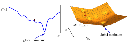
Many popular optimization techniques are based on, or are interpreted via, a gradient descent Arfken and Weber (1985), which can be understood as placing a fictitious zero-mass particle at some randomly chosen position on the energy landscape representing the cost function, and allowing this particle to spontaneously evolve towards the relevant minimum (Fig. 1). The particle behavior can be described as evolution of a state point of a gradient dynamical system (DS)
| (1) |
where is a state vector in , which in the context of optimization task becomes the vector of parameters in need of optimization. Also, is the time derivative of , i.e. , is the velocity vector field of the DS, plays the role of a scalar energy landscape function at least twice continuously differentiable Hirsch, Smale, and Devaney (2004), and is its gradient.
However, the process described by system (1) leads to the local minimum, which might not be the global one. In order to find the global minimum starting from arbitrary initial conditions, one needs to introduce into the system a mechanism to overcome the barriers between local minima. Arguably the most popular modifications of the technique above are based on adding stochastic terms in Eq. (1) or in its discrete-time analog Kushner and Clark (1978); Kirkpatrick, Gelatt Jr, and Vecchi (1983); Aluffi-Pentini, Parisi, and Zirilli (1985); Gelfand and Mitter (1991). A distinctive feature of such methods, including one of the most efficient methods called simulated annealing Kirkpatrick, Gelatt Jr, and Vecchi (1983); Aluffi-Pentini, Parisi, and Zirilli (1985), is monotonous decrease of the intensity of the applied random noise (analogue of “temperature") from some relatively large value to zero, which leads to the convergence of the solution of the respective differential or difference equation to the global minimum with reasonably large probability. With this, the barriers separating the minima are overcome thanks to random forces pushing the system over their tops. Such approaches principally require algorithmic computation and therefore digital computers.
Contrary to that, quantum computers utilize quantum annealing, i.e. the ability of a quantum system to penetrate the potential barriers between the local minima of their energy function by means of tunnelling, thus dramatically speeding up the search for the global minimum as compared to classical methods. Theoretically, this seems to be the best optimization method, however, its physical implementation is technologically highly challenging. With this, in the existing quantum devices the convergence to the global minimum (ground state) is also achievable with some probability and is therefore not guaranteed King et al. (2017). Generally, none of the optimization methods available to date are perfect, making exploration of new approaches always valuable.
Here we propose and explore an alternative principle enabling the fictitious particle to overcome the barriers between the minima by inducing global bifurcations in (1) after a simple modification. Given that differential equations are implementable in analogue electronic devices, this idea could pave the way for non-digital and non-quantum optimizers.
Namely, we propose to delay the argument of the right-hand side function in (1) by the same amount to obtain the following delay-differential equation (DDE)
| (2) |
with , , assuming that as . Here, a scalar is a single control parameter, whose modification leads to the changes in the available dynamical regimes.
Inspired by the theory of bifurcations in ordinary differential equations (ODEs) and by the knowledge of typical delay-induced effects in dynamical systems overviewed in Section II, we hypothesize that the increase of should destroy all local attractors around the minima of and create a single large attractor embracing all minima, thus forcing the phase trajectory to spontaneously visit their neighbourhoods. This way, the barriers between the minima would be effectively removed through a fully deterministic mechanism associated with global bifurcations, such as homoclinic bifurcations of fixed points and of periodic orbits. A useful overview of such homoclinic bifurcations occurring in ODEs can be found in the book from the research group of Vadim Anishchenko Anishchenko, Vadivasova, and Strelkova (2014).
Assuming that our hypothesis is true, the desirable optimization procedure would consist of launching the system (2) from arbitrary initial conditions at and waiting until it reaches one of the local minima, then slowly increasing from zero to some positive value, then slowly decreasing to zero, and watching the system converge to the global minimum automatically. This process would be somewhat similar to the simulated annealing in the sense that a control parameter would increase and subsequently decrease to lead the system to the global minimum. However, it would be dissimilar in being deterministic, which could be advantageous over probabilistic approaches of the simulated and quantum annealings, provided that it achieves the same goal.
Since a DDE could be implemented in an analogue electronic device, and the increase and decrease of a single control parameter would be equivalent to turning a handle in an experiment, the proposed scheme would potentially not require sophisticated algorithms and hence a digital computer. However, in this paper we use a digital computer to verify the concept by simulating the relevant equation numerically.
Our goal is to investigate whether the newly proposed approach is able to deliver the global minimum successfully, and if so, under what conditions. In Section II we overview the facts about DDEs, which provide the theoretical foundation for our delay-based approach to optimization. In Section III we reveal delay-induced bifurcations and demonstrate how the proposed technique works in systems with five-well landscapes of various configurations giving rise to various forms of the barrier-breaking mechanism based on global bifurcations. In Section IV we discuss the proposed approach in the context of quantum optimization and simulated annealing (often used as a benchmark for quantum optimization Denchev et al. (2016)), and indicate some of its potential advantages and limitations.
Alongside with exploring the potential applicability of DDEs for optimization, we reveal some universal behavioral features of nonlinear DDEs of the given class, and thus contribute to the general knowledge of systems with delay.
II Theoretical basis for the delay-based optimization: bifurcations
The gradient DS of the form (1) can demonstrate only two kinds of evolution: from a certain initial condition it can monotonously tend either to the fixed point located at some local minimum, or to infinity (positive or negative) if the shape of the landscape function permits Hirsch, Smale, and Devaney (2004). Importantly, it cannot demonstrate oscillations of any kind, let alone any more complex dynamics. However, it is well known that even if the DS without a delay behaves in a very regular manner, introduction of a time delay is likely to change its dynamics dramatically and to induce bifurcations leading to complex oscillations. Even a single delay term can give birth to periodic Hale (1971); Hale and Verduyn Lunel (1993), quasi-periodic and chaotic solutions Bellen and Zennaro (2003). This phenomenon occurs thanks to the expansion of the dimension of the phase space of the DS from some finite number without delay to infinity with delay.
There has been a lot of research devoted to the study of various special cases of DSs with delay modelling natural processes Hutchinson (1948); Cunningham (1954); Mackey and Glass (1977); Bocharov and Romanyukha (1994); Cooke and vandenDriessche (1996); Wolkowicz and Xia (1997); Culshaw and Ruan (2000); Smolen, Baxter, and Byrne (2001); Nelson and Perelson (2002); Ursino and Magosso (2003); Villasana and Radunskaya (2003); Dhamala, Jirsa, and Ding (2004). In most examples studied, the delay appears in the extra term(s) added to the components(s) of the velocity field of the system under study, like e.g. in Chow and Mallet-Paret (1983); Mallet-Paret and Nussbaum (1986); Chow, Lin, and Mallet-Paret (1989), or when some terms defining the velocity field are delayed and some are not Goodwin (1951); Cunningham (1954); an der Heiden and Walther (1983). With this, the effects induced by a delay greatly depend on the particular form of the DS under study and on the exact way the delay is introduced. It is impossible to predict, without resorting to numerical bifurcation analysis, how a general non-linear DS would respond if the delay is incorporated into it in some arbitrary manner.
There is a small number of rigorous theoretical results allowing one to qualitatively predict the global behavior of non-linear DDEs for special simple cases of scalar DDEs of the form with functions crossing zero not more than twice. For , this would correspond to having not more than one minimum and/or one maximum. Clearly, such cases do not represent any challenge for optimization and can be handled with the simplest gradient descent (1).
Specifically, in such systems the key phenomena that can be predicted analytically are: (i) the birth of a limit cycle localized around the minimum of Nussbaum (1973, 1974), (ii) a homoclinic bifurcation of a saddle fixed point located at the maximum of Walther (1989, 1990), and (iii) a homoclinic bifurcation of a saddle cycle around the maximum of Walther (1981); Hale and Lin (1986). In Janson and Marsden (2021) it is demonstrated that such homoclinic bifurcations ultimately lead to the disappearance of attractors born from, and localized near, the single minimum of as the delay grows.
More realistically, the function in need of optimization would have more than one minimum, and for such cases no rigorous theoretical results predicting homoclinic or other global bifurcations are available. Striving to predict bifurcations in such systems, we make the following observations. Homoclinic bifurcations are global, i.e. technically non-local, since they do not affect the stability of a saddle point or a cycle, whose manifolds close to form a homoclinic loop. However, the regions of the phase space involved in a homoclinic bifurcation are bounded thanks to the presence of nearby attractors, saddle fixed points or cycles, and/or of their manifolds. So, firstly, homoclinic bifurcations are localized in this sense. Secondly, in (2) bifurcations do not change if is translated in space, which can be easily shown by a trivial variable substitution. Thus, if a single-well is shifted in the phase space, bifurcations change their locations accordingly, but otherwise stay the same. Thirdly, a smooth multi-well cost function can be obtained by gluing together, and smoothing out at the gluing points, the segments of single-well and/or single-hump functions, for which some predictions are possible as described above.
We combine the above observations with theoretical results for single-well and/or single-hump functions , and use essentially induction to hypothesize that in (2) with a multi-well , the increase of should induce a sequence of global homoclinic-like bifurcations eliminating local attractors one by one. We envision that after all local attractors disappear, at sufficiently large there should exist a single chaotic attractor spanning all maxima and minima of , which would force the phase trajectory to approach the vicinities of all minima, including the global one. This would resemble both simulated annealing, and quantum annealing, in the sense that the delay would make the imaginary particle overcome the barriers between the local minima and hence act as a substitute for random forces or for quantum tunneling, respectively.
In Janson and Marsden (2021) global bifurcations were numerically analyzed in a scalar version of (2) with a two-well landscape . It was found that the growth of leads to a chain of three homoclinic bifurcations, which destroy attractors localized around two minima of , and to the birth of a large attractor embracing both minima. Although the nature of homoclinic bifurcations varied depending on the local features of , these were not very important in the sense that, one way or another, they caused the death of both local attractors at sufficiently large , and leaving a single large chaos embracing both minima.
Here we analyze a scalar version of (2) with a multi-well cost function , which reads
| (3) |
where , . Also, is the function of a scalar argument, such that as .
In Section III we explore and largely confirm the validity of the hypothesis about the chain of global, homoclinic or similar, bifurcations evoked by the increasing delay, which continues until all local attractors cease to exist. Note, that for a landscape with more than two wells, i.e. with more than one saddle fixed point, in addition to homoclinic bifurcations involving the same saddle point, it becomes reasonable to expect heteroclinic bifurcations involving more than one saddle point. We discuss in what situations the newly proposed procedure can deliver the global minimum of a multi-well landscape.
In what follows, we use an expression “instant of bifurcation" for brevity in order to refer to the value of the delay at which the given bifurcation occurs. All bifurcations discussed in this paper occur as increases from smaller to larger values. If we consider a fixed point at a value of smaller (or larger) than the value at which a certain bifurcation occurs, we will say that the fixed point is below (or above) the given bifurcation.
III Demonstration of principle
| Lowest minimum is flattest (), wells have simple shapes. Lowest minimum is found. | |||||||||||||||||||||||||||||||||||||||||||||
| (4) | |||||||||||||||||||||||||||||||||||||||||||||
|
|
|||||||||||||||||||||||||||||||||||||||||||||
| Lowest () and flattest () minima are different, wells have simple shapes. Flattest minimum is found. | |||||||||||||||||||||||||||||||||||||||||||||
| (5) | |||||||||||||||||||||||||||||||||||||||||||||
|
|
|||||||||||||||||||||||||||||||||||||||||||||
| Lowest (), flattest () and found () minima are different, wells have complex shapes. | |||||||||||||||||||||||||||||||||||||||||||||
| Neither lowest, nor flattest minimum is found. | |||||||||||||||||||||||||||||||||||||||||||||
| (6) | |||||||||||||||||||||||||||||||||||||||||||||
|
|
In the given section we demonstrate the performance of our delay-based
approach
using three five-well landscapes with subtly different local properties leading to noticeably different delay-induced effects, and specifically to different orders and forms of bifurcation mechanisms in which the barriers between the local minima are removed. Namely, the first two landscapes considered in Subsections III.1 and III.2 have potential wells of a relatively simple shape, such that the respective functions of (3) do not oscillate between any two consecutive zero-crossings (see red lines in Figs. 2(a) and 4(a)). In the third example analysed in Subsection III.3, some of the wells have more complex shapes, such that within them the function displays oscillations, as shown by red line in Fig. 6(a) between and .
With this, in the first example the lowest minimum is also the flattest one, whereas in the second and third examples the lowest minima are not the flattest. We will show that the proposed approach is likely to deliver the global minimum where this minimum is the flattest and the respective potential well is sufficiently wide, and the cost function is of relatively simple shape, i.e. the right-hand side of the DDE in (3) does not oscillate between consecutive zero-crossings.
III.1 Reaching the global minimum
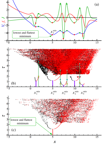
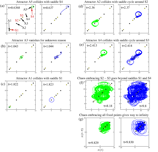
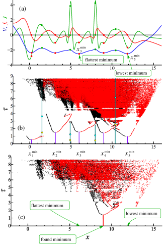
Here we consider the landscape specified by Eq. (4) from Table I and shown by blue line in Fig. 2(a). In the given function , there are five minima marked by red filled circles, and four maxima marked by green filled circles. In what follows, we will denote the minima as and the maxima as , with indices and being the numbers of the respective minimum/maximum if counted from the left, so that and . All minima together with their depths are given in Table I under Eq. (4). Although the global minimum here is , there is another minimum , which is only marginally higher and would be an almost equivalent choice for the best solution. The landscape has a relatively simple shape, so that does not oscillate between any two consecutive zero-crossings, see red line in Fig. 2(a). Below we will first reveal bifurcations occurring in this system as grows, and then the behavior of the system as slowly decreases from a large value.
At any , the equation (3) with specified by (4) has nine fixed points indicated by circles in Fig. 3(a). At , there are five stable and four unstable fixed points, both of a node type, which means that the solution approaches the former and departs the latter in a non-oscillatory manner. At , every fixed point has infinitely many pairs of complex-conjugate eigenvalues. An overview of the theoretical results related to the stability analysis of fixed points in DDEs using Lambert function is available in Asl and Ulsoy (2003). The values of at which local bifurcations of the fixed points occur are determined by the values of the Jacobian at these points. A th eigenvalue of a fixed point of (3) can be expressed in terms of the Lambert function with and as
where and is the fixed point. Note, that the function has countably many branches. Illustrations of and of the respective eigenvalues as functions of can be found e.g. in Janson and Marsden (2021).
The function is shown in Fig. 2(a) by a green line, and its values at the fixed points are indicated by red or green filled circles for the minima and maxima, respectively.
Firstly, consider local bifurcations of the fixed points at the landscape minima , at which . The values of at all minima are given in Table I under Eq. (4). For a fixed point has one real negative eigenvalue and infinitely many pairs of complex-conjugate eigenvalues with very large negative real parts. The latter implies that although is technically a stable focus, the phase trajectories approach this point in a non-oscillatory manner. For the same point has infinitely many pairs of complex-conjugate eigenvalues with negative real parts. It remains a stable focus, but here the real parts of the leading pair of eigenvalues are relatively small negative numbers, so the solution near this point oscillates.
At a value of from this point a stable limit cycle is born via the first Andronov-Hopf (AH) bifurcation. The respective values of for all minima are given in Table I below Eq. (4). In the bifurcation diagram given in Fig. 2(b), the fixed points at the minima are shown as lilac vertical lines until the values , i.e. as long as they remain stable. Above these values of they continue to exist as unstable fixed points of a saddle-focus type and are not shown. At even higher values of they undergo more AH bifurcations, which do not restore their stability and instead make them more and more unstable.
Also, in Fig. 2(b) above every point of the first AH bifurcation of , i.e. above the top of the lilac line, we show both the maxima (red dots) and the minima (black dots) of the newly born stable limit cycles. This style of presenting a bifurcation diagram is different from a conventional one, in which only one kind of an attractor extremum is usually depicted. Here we need to monitor both extrema in order to observe how a limit cycle grows in size with and eventually approaches a nearby saddle fixed point or another saddle object before vanishing in a homoclinic bifurcation, bearing in mind that the respective saddle object can exist to any side of the limit cycle. At higher values of , the limit cycles are replaced by non-periodic attractors, for which we continue to show all the local maxima and minima as they can also experience homoclinic bifurcations.
Note that at the same values of there can be more than one co-existing non-fixed point attractor. However, in Fig. 2(b) we use the same two colors black and red to depict all such attractors at the given value of . The reason is that technically it becomes quite difficult to label different attractors in the presence of so many non-local bifurcations. Therefore, the given bifurcation diagram alone does not allow one to determine either the total number of coexisting attractors, or the span of individual attractors at every value of . However, a better understanding of the sequence of bifurcations can be achieved by comparing this diagram with phase portraits in Fig. 3 described below.
Now, consider local bifurcations of the fixed points at the landscape maxima indicated by vertical green lines in Fig. 2(b), at which . From being unstable nodes at , at any positive they turn into saddle-foci because they have a finite number of pairs of complex-conjugate eigenvalues with positive real parts, and a countably infinite number of complex-conjugate eigenvalue pairs with negative real parts. With this, they can also undergo AH bifurcations. Namely, the first AH bifurcation of a saddle-focus fixed point occurs at , where is the Jacobian at this point. The values of and the respective for all maxima are given in Table I under Eq. (4). The first AH bifurcation can give rise to a saddle cycle. All four unstable fixed points are shown in Fig. 2(b) by green vertical lines for the ranges of until their respective second AH bifurcations at occurs. An exception is , for which the second AH bifurcation occurs at and is outside the range of covered by this graph. The first AH bifurcations for each point are marked by filled cyan circles, and the second AH bifurcations by empty circles on the green vertical lines.
Next, consider non-local bifurcations occurring in this system. As explained in Section II, we expect at least two kinds of homoclinic bifurcations leading to the disappearance of localized attractors. These would constitute slightly different versions of the same mechanism, based on global bifurcations, behind the elimination of the barriers between the local minima of , which are embodied in the manifolds separating the basins of attraction of localized attractors.
The simplest homoclinic bifurcation occurs when the manifolds of a saddle-focus fixed point at a landscape maximum close to form a homoclinic loop. A more complex scenario takes place if below the homoclinic bifurcation, the saddle-focus at a maximum has undergone AH bifurcation and gave birth to a saddle cycle. Then the homoclinic “loop" is formed by the manifolds of this saddle cycle rather than those of the fixed point. Note, that the unstable manifold of the saddle cycle has dimension two, rather than one in the case of the simplest saddle fixed point. The structure formed by the manifolds of the saddle cycle at the homoclinic bifurcation is more complex than the relatively simple loop created by the manifolds of the saddle point. For this reason, when describing the homoclinic bifurcation involving the saddle cycle, we refer to a “loop", rather than the loop. In either case, the end result is the disappearance of the local attractor as a result of its collision with either the saddle point, or the saddle cycle.
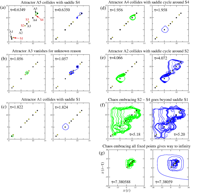
(a) Before (left) and after (right) the safe homoclinic loop of the saddle point at the maximum S4. Green line: limit cycle A5 before bifurcation. Blue line: phase trajectory starting near A5 and converging to fixed point A4 after bifurcation.
(b) Before (left) and after (right) the global bifurcation eliminating attractor A3. Green line: chaotic attractor A3 before bifurcation. Blue line: phase trajectory starting near A3 and converging to the minimum A4 after bifurcation.
(c) Before (left) and after (right) the safe homoclinic loop of the saddle point at the maximum S1. Green line: limit cycle A1 before bifurcation. Blue line: limit cycle A2 to which trajectory converges after bifurcation starting from the vicinity of A1.
(d) Before (left) and after (right) the homoclinic “loop" formed by the manifolds of the saddle cycle around the maximum S4. Green line: chaotic attractor A4 before bifurcation. Blue line: limit cycle A2 attracting the trajectory after bifurcation from the vicinity of A4.
(e) Before (left) and after (right) the homoclinic “loop" formed by the manifolds of the saddle cycle around the maximum S2. Green line: chaotic attractor A2 before bifurcation. Blue line: non-localized chaotic attractor born after the bifurcation.
(f) Before (left) and after (right) the global bifurcation giving birth to large chaos embracing all fixed points. Green line: smaller chaotic attractor before bifurcation. Blue line: large chaotic attractor born from the bifurcation.
(g) Death of the last attractor. Green line: large chaos before bifurcation. Blue line: trajectory going to infinity after bifurcation.
With this, as predicted by Shilnikov’s theorem for a homoclinic loop of a saddle-focus in ODEs Shilnikov (1965, 1968), depending on the value of its saddle quantity , before such a collision one can expect two different kinds of dynamics. Namely, , where is the positive real eigenvalue of the fixed point, and are eigenvalues with the negative real parts closest to zero. If , the homoclinic loop is expected to be “safe" and should coincide with the limit cycle at the instant of collision. This result was verified for a special form of a DDE Walther (1985, 1989). If , the loop is expected to be “dangerous", and at just below the loop formation the localized attractor should be chaotic. However, to the best of our knowledge, this was not verified for DDEs. Regardless of the kind of the homoclinic loop, the localized attractor should disappear, but in Fig. 2(b) we nevertheless indicate the values of at which the saddle quantities of all saddle-foci at the maxima of change sign from negative to positive by filled yellow circles on the vertical green lines.
We can see that the type of a homoclinic bifurcation can be predicted from the knowledge of the eigenvalues of the respective saddle point at the instant of bifurcation. However, the parameter values, at which this or any other non-local bifurcation occur, can be detected only through numerical simulations by observing the solutions. Therefore, we reveal all non-local bifurcations in (3) with the landscape (4) by looking at the phase portraits projected on the plane , . In Fig. 3, panels (a)–(g) illustrate such bifurcations one by one in the order of their occurrence as increases. Each panel shows all fixed points of the system, with black circles indicating the landscape minima , which can be stable or unstable at different , and yellow circles indicating always unstable points at the landscape maxima . Note, that all fixed points lie on the diagonal . For the ease of reference, in (a) we label all the landscape maxima as S with , and all attractors at or around the minima as A with . In each panel, the green line in the left-hand part shows an attractor about to disappear as a result of a bifurcation; the blue line in the right-hand part of the same panel shows an attractor to which the system converges after the bifurcation from the initial conditions where the vanished attractor was. The exceptions here are panels (a)–(b), whose right-hand parts show the whole trajectories converging to the fixed points, rather than the resultant fixed points only. The respective values of are given in the fields of every phase portrait. Note, that in (a)–(d) there might co-exist oscillatory attractors not involved in the given homoclinic bifurcation, but these are not shown to avoid confusion.
The first homoclinic bifurcation occurs when the limit cycle A5 (green line in (a)), born at around , is the first to collide with the nearest saddle S4 at to form a homoclinic loop. As seen from Fig. 2(b), this collision occurs before the saddle quantity turns positive, so the homoclinic loop is “safe". After attractor A5 vanishes, the phase trajectory (blue line in (a)) goes to the neighbouring attractor A4, which is the stable fixed point .
The second non-local bifurcation is associated with a sudden disappearance of a chaotic attractor A3 around (green line in Fig. 3(b)). No collision with any saddle-focus is observed here. Moreover, from Fig. 2(b) one can see that no saddle cycles were born from the nearby saddle-foci S2 and S3 before this global bifurcation, since both S2 and S3 are below the first AH bifurcation at . Thus, there could be no collision with a saddle cycle either. We can only hypothesize that some heteroclinic connection might be involved, in which a manifold of one saddle object connects to another saddle object, but we cannot verify this here. In any case, the second localized attractor disappears as a result of a non-local bifurcation at , and the phase trajectory (blue line in (b)) goes to the stable fixed point A4. Note, that although underwent AH bifurcation before (see Table I), the attractor A3 vanishes only after A5 because its potential well is wider.
The third non-local bifurcation occurs at to the limit cycle A1 (green line in (c)) born from at . This bifurcation is of the simplest type since the saddle quantity is negative. After the bifurcation, the phase trajectory converges to the closest attractor A2, which is a limit cycle (blue line in (c)).
Next, at disappears an attractor A4 (green line in (d)). Note, that at the instant of homoclinic bifurcation, the relevant saddle point S4 at is above the first AH bifurcation, which implies that there is a saddle cycle around , whose co-dimension-one (infinite-dimensional) stable and two dimensional unstable manifolds form the relevant homoclinic “loop". The attractor about to vanish in the bifurcation is chaotic (compare with simpler cases in Janson and Marsden (2021)). Above this homoclinic bifurcation there remains no attractor localized around , and the phase trajectory starting from its vicinity goes to the limit cycle A2 (blue line in (d)).
The last local attractor to disappear is A2, which at collides with a saddle cycle born from the saddle S2 and is therefore chaotic before this collision (green line in (e)). Above this bifurcation, no localized attractors are left. However, a larger attractor embracing all fixed points except and is formed (blue line in (e)) presumably due to an intersection of some manifolds or some heteroclinic connection. As grows further, this attractor goes beyond the saddle (green and blue lines in (f)). A large attractor spanning all fixed points exists for a relatively large range of values, and it remains chaotic for most of this range, as seen from Fig. 3(b)). However, at the final non-local bifurcation occurs, which destroys the basin of attraction of this large chaos, and the phase trajectory goes to infinity (blue line in (g)).
Note, that the last localized attractor to disappear here is around , which is the lowest and the flattest minimum whose potential well is wide enough (see blue line in Fig. 3(a)). The largest flatness (the smallest value of ) of this minimum ensures that the limit cycle is born from it at the largest value of as compared to other minima. The sufficiently large distance between this minimum and the nearest edge of the respective well ensured that for the attractor born from the minimum there is sufficient room to grow in size before disappearing, and thus to outlive all other localized attractors as grows.
Now, when running the simulation from the initial conditions on the large chaotic attractor at some sufficiently large value of , and slowly decrease to zero, as illustrated in Fig. 2(c), the phase trajectory ends up at the lowest minimum automatically, as desired within an ideal global optimization scenario.
III.2 Reaching the flattest minimum
(a) Before (left) and after (right) the safe homoclinic loop of the saddle point S4 (similar to Fig. 3(a)). Green line: limit cycle A5 before bifurcation. Blue line: phase trajectory starting near A5 and converging to the minimum A4 after bifurcation.
(b) Before (left) and after (right) the global bifurcation eliminating attractor A3 (similar to Fig. 3(b)). Green line: chaotic attractor A3 before bifurcation. Blue line: phase trajectory starting near A3 and converging to the minimum A4 after bifurcation.
(c) Before (left) and after (right) the safe homoclinic loop of the saddle point S1 (similar to Fig. 3(c)). Green line: limit cycle A1 before bifurcation. Blue line: limit cycle A2 to which trajectory converges after bifurcation starting from the vicinity of A1.
(d) Before (left) and after (right) the homoclinic “loop" formed by the manifolds of the saddle cycle around S2 (different from Fig. 3(d)). Green line: chaos A2 before bifurcation. Blue line: chaos A4 attracting the trajectory after bifurcation from the vicinity of A2.
(e) Before (left) and after (right) the homoclinic “loop" formed by the manifolds of the saddle cycle around S3 (different from Fig. 3(e)). Green line: chaotic attractor A4 before bifurcation. Blue line: non-localized chaotic attractor born after the bifurcation.
(f) Before (left) and after (right) the global bifurcation giving birth to large chaos embracing all fixed points (similar to Fig. 3(f)). Green line: smaller chaotic attractor before bifurcation. Blue line: large chaotic attractor born from the bifurcation.
(g) Death of the last attractor (similar to Fig. 3(g)). Green line: large chaos before bifurcation. Blue line: trajectory going to infinity after bifurcation.
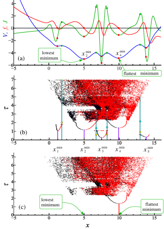
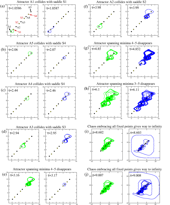
In the example considered here, is designed in order to achieve a different order of deaths of the localized attractors as increases, comparing to (4), by appropriately adjusting the flatnesses, depths and locations of the relevant minima, as described below. The landscape is specified by Eq. (5) and given by blue line in Fig. 4(a). Similarly to the landscape described by (4) and considered in Sec. III.1, here there are five minima. Four of these minima, namely to , are at approximately the same positions, and their respective potential wells are of approximately the same width as in (4). Inside each well of , the function of (3) (red line in Fig. 4(a)) does not oscillate, so the shape of is relatively simple.
The global minimum is still , however, it is no longer the flattest of all minima. The minimum is slightly higher than and also slightly flatter, i.e. its is slightly smaller (see Table I below Eq. (5)). With this, because is now located further to the right than in (5), the distances from both and to their respective nearest well edges are very close.
Figure 4 has the same structure and notations as Fig. 2. One can see that the bifurcation diagram in (b) is qualitatively similar to the one of Fig. 2(b), and all the same bifurcations are taking place here as increases, albeit in a slightly different order and at different values of . This is also evident from comparing Figs. 3 and 5 where the non-local bifurcations are illustrated with the phase portraits.
The most important distinction from the case of Sec. III.1 is that the last localized attractor surviving at the higest value of is chaos A4 around . In Fig. 5(e) green line in the left part shows this attractor just before the homoclinic bifurcation at , and blue line in the right part shows the attractor to which the phase trajectory converges after the homoclinic bifurcation at , which is chaos spanning three minima and two maxima. The homoclinic bifurcation occurs at and consists of the closure of manifolds of the saddle cycle around (S3).
After the disappearance of all localized attractors, the further increase of leads to the further growth of the single large chaotic attractor, until it goes beyond the outermost maxima as illustrated in Fig. 5(g) and ends up spanning all fixed points. With this, the growth of this single remaining attractor is limited by the final non-local bifurcation at , after which the phase trajectory tends to infinity (Fig. 5(f)).
If we launch the system from the initial conditions on the large chaotic attractor at , and its behavior is observed as slowly decreases to zero, the system converges to the non-global minimum , which is the flattest minimum, as illustrated in Fig. 4(c).
III.3 Reaching an arbitrary minimum
Here we construct an example of with the same number of minima as in previously considered cases (4) and (5), but with a more intricate shape of some wells. By doing so, we assess whether the enhanced non-linearity of the system is likely to disrupt the hypothesized and provisionally verified chain of delay-induced global bifurcations destroying local attractors one by one, leading to global chaos at large values of , and thus removing the barriers that without the delay prevented the phase trajectory from approaching some (most) minima of .
We are also interested in testing the proposed approach to optimization in the difficult situation where the deepest wells are only subtly different in their depths. The landscape meeting the above requirements is specified by (6) in Table I and shown by blue line in Fig. 6(a). Here, just like in the previous two cases considered, has five minima. However, in the range the function demonstrates small oscillations between consecutive pairs of zero-crossings, which make the respective DDE considerably more nonlinear. The depths of the five local minima are only slightly different from each other (see Table I below Eq. (6)), and the global minimum is only slightly lower than the other minima.
As grows, all five fixed points – undergo AH bifurcations and give birth to stable limit cycles, which grow in size with in full analogy with the previous cases considered, as illustrated in Fig. 6(b).
However, non-local bifurcations occur in a less predictable manner than with previous examples. In what follows, we indicate similarities and distinctions from the cases considered above in the scenarios developing as grows.
We start from listing the similarities. Firstly, all five localized attractors disappear through the homoclinic bifurcations in the same manner as before, as illustrated in Figs. 7(a)–(d) and (f). With this, the nature of the homoclinic bifurcation is determined by whether the relevant saddle-focus fixed point was before or after the first AH bifurcation. Namely, in (a)–(c) the limit cycles born from , and collide with the saddle-foci and and form safe homoclinic loops, because the latters are not only below their first AH bifurcations, but also below the instants where their saddle quantities become positive. On the other hand, (d) and (f) illustrate homoclinic bifurcations representing the closures of manifolds of saddle cycles born from and , respectively.
Note, that in the given landscape , and are much sharper than in (4) and (5), as can be seen from the high splashes of function in Fig. 6(a) (green line). The high values of lead to AH bifurcations of these fixed points occurring at much smaller values of than in both previous examples. However, the homoclinic bifurcations involving manifolds of the saddle cycles around these maxima occur in the same manner as in the previous two examples (compare Figs. 7(d), (f) with e.g. Figs. 5(d)–(e)), although at the instants of homoclinic collisions both and are already above the second AH bifurcation.
The second similarity is that at a sufficiently large , the system possesses a single large chaotic attractor embracing all fixed points (compare the left parts of Figs. 7(i)–(j) with those of Figs. 3(g) and 5(g)). Thirdly, at even larger , this large chaos disappears too, and the system goes to infinity (compare the right part of Fig. 7(j) with those of Figs. 3(g) and 5(g)). Finally and perhaps most importantly, as could be expected from the previous argument and in agreement with previous cases, the localized attractor surviving at the largest value of is A2 whose potential well is the flattest and of a similar width with other wells (see Fig. 7 (f)).
Next, we describe the distinctions from the relatively predictable scenarios involving relatively simple shapes of given by (4) and (5). Firstly, unlike in the case above, here attractors involving two or more minima can coexist with attractors localized around a single minimum. Namely, in Figs. 7(c)–(f) one can see a chaotic attractor spanning minima and , which exists while the localized attractors A2, A3 and A4 are not yet destroyed via homoclinic bifurcations.
Secondly, as seen from Figs. 6(b) and 7, in homoclinic bifurcations involving –, counterintuitively, the localized attractor collides with the saddle object (point or cycle), which is not the closest to the minimum from which this attractor had originated. For example, Fig. 7(d) shows an attractor A3 around undergoing a homoclinic bifurcation with the saddle cycle around S3 at , although and the saddle cycle around it are both located closer.
Thirdly, and most significantly, the minimum attracting the system while slowly decreases from the value of is not the one which survives at the largest value of , i.e. not , as can be seen from Fig. 6(c). Instead, it is the , whose homoclinic bifrucation with the saddle-focus S4 at gave rise to the chaotic attractor embracing and (see blue line in Fig. 7(c)). The reason is that the large chaos shown in the left part of (i) develops from the latter attractor as grows. When at the phase trajectory is launched from the only attractor available, as decreases, this chaotic attractor undergoes a cascade of non-local bifurcations, as a result of which it becomes confined within the smaller and smaller number of minima. As a result, the phase trajectory does not go beyond (S3) since it settles down on the attractor A4 (see green line in (c)), which exists for all values of up to zero.
Interestingly, at above the basin of attraction of large chaos seems to become very close to the attractor itself, and is apparently quite riddled, since a very small disturbance of initial conditions can lead to the phase trajectory going to infinity even before the attractor disappears completely at , as illustrated in Figs. 7(i).
The attractors spanning more than one minimum appear here despite the existence of localized attractors. By analogy with similar phenomena in ODEs Li and Moon (1990), it is reasonable to suggest that they could be born as a result of repeated formation of homoclinic loops and heteroclinic connections. Just like in the previous simpler cases, here there is an abundance of saddle objects with manifolds attached to them, which can potentially form loops and heteroclinic connections. However, due to the complex shape of , the probability of a homoclinic or a heteroclinic bifurcation at any given value of seems to be higher here.
The current example, deliberately constructed as a difficult case, is an excellent illustration that in nonlinear systems with delay, it is generally impossible to predict, before performing numerical bifurcation analysis, the behavior as the delay varies. However, it is remarkable that in its most essential part, the predicted scenario is realized even despite the enhanced complexity of the nonlinear function in the DDE (3), provided that is a smooth multi-well function going to infinity outside the domain containing the extrema.
(a)/(b) Before (left) and after (right) the safe homoclinic loop of the saddle point at the maximum S1/S4. Green line: limit cycle A1/A5 before bifurcation. Blue line: phase trajectory starting near A1/A5 and converging to fixed point A2/ limit cycle A4 after bifurcation.
(c) Before (left) and after (right) the safe homoclinic loop of the saddle point S4. Green line: limit cycle A4 before bifurcation. Blue line: non-localized attractor attracting trajectory from the vicinity of A4.
(d) Before (left) and after (right) the homoclinic “loop" formed by the manifolds of the saddle cycle around S3 (similar to Fig. 5(e)). Green line: chaos A3 before bifurcation. Blue line: non-localized chaos attracting the trajectory after bifurcation from the vicinity of A3.
(e) Temporary disappearance of the first non-localized attractor (see gap in Fig. 6(b)). Green line: non-localized chaos before bifurcation. Blue line: limit cycle A4 attracting the trajectory from where chaos was at .
(f) Before (left) and after (right) the homoclinic “loop" formed by the manifolds of the saddle cycle around S2. Green line: last localized attractor A2. Blue line: reappeared non-localized chaos (compare with (d)).
(g)/(h) Smaller non-localized attractors replaced by bigger ones. Smaller chaos before (green line) and larger chaos after (blue line) bifurcation.
(i) Sensitivity to initial conditions and parameters. Green line: large chaos. Blue line: trajectory goes to infinity after a tiny change in .
(j) Death of the last attractor. Green line: large chaos before bifurcation. Blue line: trajectory goes to infinity after bifurcation.
III.4 Summary of findings
Here we summarize the results reported in the three examples considered in Sections III.1, III.2 and III.3, which illustrate different mechanisms of barrier-breaking between the local minima. We reiterate that generally it is impossible to predict without numerical analysis the behavior of nonlinear systems with delay as the delay changes, as illustrated particularly well by the case of Section III.3. However, for delay systems in a special form (3) with being a multi-well landscape tending to positive infinity as goes to infinity, it appears possible to make certain qualitative predictions with regard to the bifurcations occurring as the delay increases. Firstly, as has been well known for general delay equations, one can accurately predict the values of , at which local Andronov-Hopf bifurcations occur for all fixed points. Also, in the systems of the form (3) with single-well and/or single-hump it is possible to predict the occurrence of a non-local homoclinic bifurcation with the growth of to some extent, although the exact value of cannot be predicted and the exact form of this bifurcation can be determined only when the respective is known at least approximately. For systems with multi-well landscapes, we envisioned that localized attractors growing in size with would eventually collide with saddle objects and their manifolds in non-local bifurcations.
However, although non-local bifurcations are quantitatively unpredictable, some qualitative universal phenomena induced by such bifurcations have been hypothesized and revealed in all three cases considered. Note, that that all attractors grow in size with the delay until they experience some non-local bifurcation and vanish. Thus, the first effect is the disappearance of all attractors localized around the minima of as the delay increases, with the typical reason behind their disappearance being a homoclinic bifurcation involving the manifolds of a nearby saddle-focus fixed point or a saddle cycle. The second phenomenon is the existence of a single attractor spanning all minima of at sufficiently large values of , which is chaotic for most at which it exists. The third phenomenon is disappearance of all attractors as exceeds a certain threshold, which is different in different systems.
Besides the coexistence of attractors confined to different wells of , a typical phenomenon is the coexistence of attractors within the same well. Some of these cases were illustrated for single- and two-well cases in Janson and Marsden (2021), but we are not focussing on them specially here because they do not play a significant role in the system behavior when is decreased slowly. Also, the coexistence of attractors spanning more than one well is possible, particularly with complex shapes of , such as the one considered in Section III.3.
Generally, in the class of delay systems considered here, besides Andronov-Hopf bifurcation, the key role is played by the numerous manifolds of the saddle fixed points and saddle cycles, whose tangencies and closures induce dramatic changes in the system behavior.
In addition to possessing five local minima, the three cases of the landscape function considered here have one more feature in common, namely, as tends to , they asymptotically tend to the function , where and are some real constants. However, the universality of the phenomena presented here is confirmed by our consideration of several other forms of the landscape function with different asymptotic behaviors, which we do not report in this paper because of the limited space.
Note, that the original idea of the given research has been to investigate the applicability of delay-induced bifurcations to global optimization. The hypothesized bifurcation scenario was partly verified and partly clarified here. With this, it appears that the delivery of the global minimum with this approach is possible if the shape of the cost function in the vicinity of this minimum satisfies certain conditions, and if the shapes of all potential wells of are not too complex. Namely, the first two cases demonstrate that in the absence of oscillations of within individual potential wells of , the slow decrease of from a large value to zero makes the system converge to the minimum, which is the flattest and is far enough from the nearest maximum. This would be the minimum around which a localized attractor survives at the largest value of . If such a minimum is global, then the proposed procedure will deliver the global minimum.
IV Discussion
To summarize, we conceived a phenomenological mathematical model of a non-quantum analogue optimizer based on a previously unknown principle behind overcoming the barriers between the minima of the cost function, namely, global bifurcations caused by time delay. We proved the principle by numerical simulations of a scalar version of the model (2), and explored the possible theoretical limitations of this approach. As a key prerequisite to our approach, based on a highly limited number of relevant rigorous theoretical results available for non-linear delay equations, we formulated a hypothesis about the inevitability of a chain of global attractor- and barrier-destroying bifurcations caused by the increase of delay. Further research would be needed in order to test this approach with non-scalar versions of (2) and with more realistic tasks to solve. If its workability is confirmed, it would be interesting to implement the same principle with analogue electronic circuits, which could potentially be more efficient than digital computers in such specialized tasks.
Like in many earlier works, while developing an approach for global optimization, we introduced an extension of the famous gradient descent method described by Eq. (1), in which the role of the landscape is played by the cost function. However, unlike in previous works, which used stochastic perturbations of the relevant evolution equation and employed probabilistic approaches, our trial approach described by (2) is entirely deterministic and extremely simple in its setting. Namely, we delay the argument of the right-hand side of the “gradient descent" differential equation by a certain amount , which becomes the only control parameter in the system.
We assume that the optimization technique should start from launching the system (2) from arbitrary initial conditions at zero and waiting until it reaches one of the local minima, then increasing slowly until we observe the birth of a large attractor and its subsequent disappearance, and noting the respective value of . The procedure should be repeated until reaches the value just below the disappearance of the global attractor. After that, in an ideal scenario, a slow decrease of to zero would automatically bring the system to the global minimum of the cost function. Here we revealed the conditions under which this scenario could be possible.
Just like the simulated and quantum annealings, our approach involves overcoming the potential barriers separating local minima of the cost function. However, it uses a different principle to achieve this. Namely, in simulated annealing the fictitious massless particle is pushed over the maxima, in quantum annealing the barriers can be in addition penetrated using tunnelling effect Denchev et al. (2016), and in our delay-based method the barriers are effectively removed via global bifurcations.
Specifically, we revealed that in a scalar version (3) of (2) the key phenomenon is homoclinic bifurcation, which occurs repeatedly as the delay increases. The role of the homoclinic bifurcation is to eliminate, one by one, all attractors localized around the minima of the landscape as the delay grows, and to ultimately give rise to a single chaotic attractor spanning all local minima at some moderately large value of the delay.
The homoclinic bifurcation in the system considered comes in at least two varieties depending on whether the relevant saddle point located at the maximum of the landscape has undergone Andronov-Hopf bifurcation or not. However, in the context of global optimization, the exact form of a particular homoclinic bifurcation is not essential since, regardless of its form, it results in the breakdown of the localized attractor. With this, the localized attractors can disappear through mechanisms not immediately associable with the homoclinic bifurcations, for example in Figs. 3(b) and 5(b).
Based on the results of our analysis of (3) with several smooth landscapes , which were constructed to specification in order to assess various versions of the barrier-breaking mechanism operating in various orders, we conclude that the delay-induced chain of homoclinic and other global bifurcations destroying local attractors is a universal scenario, whose details depend on the shape of the particular function , but whose existence is independent of the latter.
Standard optimization tools, including simulated annealing, require algorithmic decision-making at numerous stages of the procedure and thus rely on the provision of a digital computer. It is certainly possible to simulate a continuous-time system with delay on a computer, as we do here. However, we note that the proposed approach exploits spontaneous behavior of a dynamical system, which would emerge in an underlying physical device thanks to its inner structure, just like oscillations of a pendulum in a “grandfather clock". This approach does not require continual decision-making dependent on the previous step, and hence does not need to rely on a digital computer. It could be implemented in a non-quantum analogue device with a delay, which could be designed to have a high evolution rate and hence achieve a solution reasonably quickly.
By analogy with optimization techniques based on stochastic extensions of gradient descent, it is impossible to guarantee the convergence of (2) to the global minimum of by slowly decreasing to zero due to the general impossibility to predict the behavior of nonlinear systems. However, if the global minimum is also the flattest and the respective well is wide enough, as grows, the attractor around it is likely to be destroyed last. If the wells of the cost function are not too complex in their shape, as decreases from the positive value, at which global chaos exists, to zero, the system is likely to end up at the global minimum.
Note, that the above conditions are quite consistent with those for quantum computers, in which the possibility to achieve a global minimum depends on the shape of the energy landscape Denchev et al. (2016). With this, the implementability of the proposed principle with analogue electronic devices could be an advantage over quantum computers, which although expected to be the best optimizers in theory, are difficult and expensive to make in practice. Therefore, this approach deserves to be explored further as an interesting alternative to the available techniques for global optimization.
Obviously, it will be very important to assess the efficiency of the proposed approach by applying it to more realistic challenging problems, and by comparing its performance with that of the standard optimization methods, which will be the subject of future work.
In addition to probing a novel approach to optimization, our paper contributes to the theory of nonlinear delay differential equations (DDEs) by considering their special class and revealing a universal scenario that unfolds as the delay is increased. Despite the high nonlinearity of the DDEs considered, we show that it is possible to make some qualitative predictions about their behavior.
In order to improve our understanding of the delay-induced effects in the nonlinear systems of the given class, it would be desirable to verify some of the qualitative predictions and numerical observations made here with more rigorous approaches. For example, it would be important to rigorously address the seeming absence of any attractors at sufficiently large values of delay, or the existence of a single global attractor embracing all fixed points at some moderate delays. Lyapunov functionals could be promising for this purpose, although identification of suitable functionals is not straightforward here. Addressing these questions would be an interesting task for the future.
V Authors’ contributions
NBJ proposed the research, analysed systems illustrated in the paper, interpreted the results, and wrote the paper. CJM carried out preliminary testing of the initial hypothesis with examples not illustrated in the paper, and edited the paper. Both authors contributed to the design of research.
VI Data availability
Data sharing is not applicable to this article as no new data were created or analyzed in this study.
VII Acknowledgements
The authors are grateful to Alexander Balanov for help in creating software to solve DDEs numerically and for helpful feedback on the draft of the paper, and to Alexander Zagoskin for the discussions of quantum annealing. CJM was supported by EPSRC (UK) during his PhD studies in Loughborough University, grant EP/P504236/1.
References
- Horst and Pardalos (1995) R. Horst and P. Pardalos, Handbook of Global Optimization (Springer, 1995).
- Pardalos and Romeijn (2002) P. Pardalos and H. Romeijn, Handbook of Global Optimization, Vol. 2 (Kluwer Academic Publishers, 2002).
- Floudas and Gounaris (2009) C. Floudas and C. Gounaris, “A review of recent advances in global optimization,” Journal of Global Optimization 45, 3–38 (2009).
- Floudas and P.M. (2008) C. Floudas and P. P.M., Encyclopedia of Optimization, 2nd Ed. (Springer, 2008).
- Vichik and Borrelli (2014) S. Vichik and F. Borrelli, “Solving linear and quadratic programs with an analog circuit,” Computers & Chemical Engineering 70, 160–171 (2014), manfred Morari Special Issue.
- King et al. (2017) J. King, S. Yarkoni, J. Raymond, I. Ozfidan, A. King, M. Mohammadi Nevisi, J. Hilton, and C. McGeoch, “Quantum annealing amid local ruggedness and global frustration,” Tech. Rep. (D-Wave Technical Report Series, 14-1003A-C, 2017).
- Arfken and Weber (1985) G. Arfken and H. Weber, Mathematical Methods for Physicists, 6th ed. (Academic Press, 1985) pp. 489–495.
- Hirsch, Smale, and Devaney (2004) M. Hirsch, S. Smale, and R. Devaney, Differential equations, dynamical systems, and an introduction to chaos (Academic Press Boston, 2004).
- Kushner and Clark (1978) H. Kushner and D. Clark, Stochastic Approximation Methods for Constrained and Unconstrained Systems, Applied Math. Science Series 26 (Springer, 1978).
- Kirkpatrick, Gelatt Jr, and Vecchi (1983) S. Kirkpatrick, C. Gelatt Jr, and M. Vecchi, “Optimization by simulated annealing,” Science 220, 671–680 (1983).
- Aluffi-Pentini, Parisi, and Zirilli (1985) F. Aluffi-Pentini, V. Parisi, and F. Zirilli, “Global optimization and stochastic differential equations,” Journal of Optimization Theory and Applications 47, 1–16 (1985).
- Gelfand and Mitter (1991) S. Gelfand and S. Mitter, “Recursive stochastic algorithms for global optimization in ,” SIAM J. Control Optim. 29, 999–Äì1018 (1991).
- Anishchenko, Vadivasova, and Strelkova (2014) V. Anishchenko, T. Vadivasova, and G. Strelkova, Deterministic Nonlinear Systems (Springer, Cham., 2014).
- Denchev et al. (2016) V. S. Denchev, S. Boixo, S. V. Isakov, N. Ding, R. Babbush, V. Smelyanskiy, J. Martinis, and H. Neven, “What is the computational value of finite-range tunneling?” Phys. Rev. X 6, 031015 (2016).
- Hale (1971) J. Hale, Functional differential equations (Springer-Verlag New York, 1971).
- Hale and Verduyn Lunel (1993) J. Hale and S. Verduyn Lunel, Introduction to functional differential equations, Vol. 99 (Springer, 1993).
- Bellen and Zennaro (2003) A. Bellen and M. Zennaro, Numerical Methods for Delay Differential Equations (Oxford University Press, 2003).
- Hutchinson (1948) G. Hutchinson, “Circular casual systems in ecology,” Annals of the New York Academy of Sciences 50, 221–246 (1948).
- Cunningham (1954) W. J. Cunningham, “A nonlinear differential-difference equation of growth,” Proceedings of the National Academy of Sciences of the United States of America 40, 708–713 (1954).
- Mackey and Glass (1977) M. Mackey and L. Glass, “Oscillation and chaos in physiological control systems,” Science 197, 287–289 (1977).
- Bocharov and Romanyukha (1994) G. Bocharov and A. Romanyukha, “Mathematical model of antiviral immune response. iii. influenza a virus infection,” J Theor Biol 167, 323–360 (1994).
- Cooke and vandenDriessche (1996) K. Cooke and P. vandenDriessche, “Analysis of an seirs epidemic model with two delays,” J of Mathematical Biology 35, 240–260 (1996).
- Wolkowicz and Xia (1997) G. Wolkowicz and H. Xia, “Global asymptotic behavior of a chemostat model with discrete delays,” SIAM J on Applied Mathematics 57, 1019–1043 (1997).
- Culshaw and Ruan (2000) R. Culshaw and S. Ruan, “A delay-differential equation model of hiv infection of cd4+ t-cells* 1,” Mathematical biosciences 165, 27–39 (2000).
- Smolen, Baxter, and Byrne (2001) P. Smolen, D. Baxter, and J. Byrne, “Modeling circadian oscillations with interlocking positive and negative feedback loops,” J of Neuroscience 21, 6644–6656 (2001).
- Nelson and Perelson (2002) P. Nelson and A. Perelson, “Mathematical analysis of delay differential equation models of hiv-1 infection,” Mathematical Biosciences 179, 73–94 (2002).
- Ursino and Magosso (2003) M. Ursino and E. Magosso, “Role of short-term cardiovascular regulation in heart period variability: a modeling study,” Am J of Physiology – Heart and Circulatory Physiology 284, H1479–H1493 (2003).
- Villasana and Radunskaya (2003) M. Villasana and A. Radunskaya, “A delay differential equation model for tumor growth,” J of Mathematical Biology 47, 270–294 (2003).
- Dhamala, Jirsa, and Ding (2004) M. Dhamala, V. Jirsa, and M. Ding, “Enhancement of neural synchrony by time delay,” Phys Rev Lett 92, 074104 (2004).
- Chow and Mallet-Paret (1983) S.-N. Chow and J. Mallet-Paret, “Singularly perturbed delay-differential equations,” in Coupled Nonlinear Oscillators, Proceedings of the Joint U.S. Army-Center for Nonlinear Studies Workshop, held in Los Alamos, North-Holland Mathematics Studies, Vol. 80, edited by J. Chandra and A. Scott (North-Holland, 1983) pp. 7–12.
- Mallet-Paret and Nussbaum (1986) J. Mallet-Paret and R. D. Nussbaum, “Global continuation and asymptotic behaviour for periodic solutions of a differential-delay equation,” Annali di Matematica Pura ed Applicata 145, 33–128 (1986).
- Chow, Lin, and Mallet-Paret (1989) S.-N. Chow, X.-B. Lin, and J. Mallet-Paret, “Transition layers for singularly perturbed delay differential equations with monotone nonlinearities,” Journal of Dynamics and Differential Equations 1, 3–43 (1989).
- Goodwin (1951) R. Goodwin, “The nonlinear accelerator and the persistence of business cycles,” Econometrica 19, 1–17 (1951).
- an der Heiden and Walther (1983) U. an der Heiden and H.-O. Walther, “Existence of chaos in control systems with delayed feedback,” Journal of Differential Equations 47, 273–295 (1983).
- Nussbaum (1973) R. Nussbaum, “Periodic solutions of some nonlinear, autonomous functional differential equations. ii,” Journal of Differential Equations 14, 360–394 (1973).
- Nussbaum (1974) R. Nussbaum, “Periodic solutions of some nonlinear autonomous functional differential equations.” Annali di Matematica 101, 263–306 (1974).
- Walther (1989) H.-O. Walther, “Homoclinic and periodic solutions of scalar differential delay equations,” Dynamical systems and ergodic theory, Banach Center Publications 23, 243–263 (1989).
- Walther (1990) H.-O. Walther, Bifurcation from a saddle connection in functional differential equations: An approach with inclination lemmas (Instytut Matematyczny Polskiej Akademi Nauk, 1990).
- Walther (1981) H.-O. Walther, “Homoclinic solution and chaos in x’(t)=f(x(t-1)),” Nonlinear Analysis: Theory, Methods & Applications 5, 775–788 (1981).
- Hale and Lin (1986) J. Hale and X.-B. Lin, “Examples of transverse homoclinic orbits in delay equations,” Nonlinear Analysis: Theory, Methods & Applications 10, 693–709 (1986).
- Janson and Marsden (2021) N. Janson and C. Marsden, “Delay-induced homoclinic bifurcations in modified gradient bistable systems and their relevance to optimization,” Chaos 31, 093120 (2021).
- Asl and Ulsoy (2003) F. M. Asl and A. G. Ulsoy, “Analysis of a system of linear delay differential equations,” ASME J. Dyn. Sys., Meas., Control. 125, 215–223 (2003).
- Shilnikov (1965) L. Shilnikov, “A case of the existence of a denumerable set of periodic motions,” Dokl. Akad. Nauk SSSR 160, 558–561 (1965).
- Shilnikov (1968) L. Shilnikov, “On the generation of a periodic motion from trajectories doubly asymptotic to an equilibrium state of saddle type,” Mathematics of the USSR-Sbornik 6, 427 (1968).
- Walther (1985) H.-O. Walther, “Bifurcation from a heteroclinic solution in differential delay equations,” Transactions of the American Mathematical Society 290, 213–233 (1985).
- Li and Moon (1990) G. Li and F. Moon, “Criteria for chaos of a three-well potential oscillator with homoclinic and heteroclinic orbits,” J. Sound Vib 136, 17–34 (1990).