Mathematical analysis and numerical solution of models with dynamic Preisach hysteresis

Abstract

Hysteresis is a phenomenon that is observed in a great variety of physical systems, which leads to a nonlinear and multivalued behavior, making their modeling and control difficult. Even though the analysis and mathematical properties of classical or rate-independent hysteresis models are known, this is not the case for dynamic models where current approaches lack a proper functional analytic framework which is essential to formulate optimization problems and develop stable numerics, both being crucial in practice. This paper deals with the description and mathematical analysis of the dynamic Preisach hysteresis model. Toward that end, we complete a widely accepted definition of the dynamic model commonly used to describe the constitutive relation between the magnetic field H and the magnetic induction B, in which, the values of B not only depends on the present values of H but also on the past history and its velocity. We first analyze mathematically some important properties of the model and compare them with known results for the static Preisach model. Then, we consider a parabolic problem with dynamic hysteresis motivated by electromagnetic field equations. Under suitable assumptions, we show the well posedness of a weak formulation of the problem and solve it numerically. Finally, we report a numerical test in order to assess the order of convergence and to illustrate the behavior of the numerical solution for different configurations of the dynamic Preisach model.

1 Introduction

Hysteresis is a nonlinear behavior exhibited by some media characterized by a special memory-based property according to which their response to particular changes is a function of the preceding responses. This characteristic is known as memory effect. A survey of hysteresis models may be found, for instance, in [29, 20, 42]. Detailed studies of these models have been done by different authors. From the mathematical point of view, we refer to the pioneering work of Krasnosel’skiĭ and Pokrovskiĭ [23], who introduced the fundamental concept of hysteresis operator and conducted a systematic analysis of the mathematical properties of these objects.

Models of hysteresis can be divided into two main classes: static or rate-independent and dynamic or rate-dependent models. In static models, the values of output depend just on the range of the input and on the order in which values have been attained; in particular, the speed of the input has no influence [41]. As a consequence, the model cannot reflect the dependence with frequency or field waveform. This is a fundamental property of classical hysteresis phenomenon; in this sense, static models are also known as rate-independent models and some authors [41] define hysteresis as a rate-independent memory only. Conversely, in dynamic hysteresis, the effect of the speed of changes of the applied input is added to the model. That is why dynamic models are also known as rate-dependent models.

The hysteresis phenomenon has been observed for a long time in many different areas of science and engineering. The term was initially coined in the area of magnetism [17] given that many ferromagnetic materials present hysteresis behavior that is reflected in the magnetization curves describing the magnetic response of the material to an applied magnetic field. From the electrical engineering point of view, having a good hysteresis model is fundamental to, for instance, correctly estimate the energy losses in electrical machines, a very important characteristic to take into account when designing an electrical device; in particular, the so-called hysteresis and excess losses [3]. Consequently, building a mathematical model of this relation is a very important (and difficult) task and numerical simulation of devices involving ferromagnetic materials is still quite a challenge.

One the of the most popular hysteresis operators among scientists and engineers is the classical Preisach model [35], a rate-independent model based on physical assumptions motivated by the concept of magnetic domains. Even if this model was first suggested in the area of ferromagnetism [32, 7, 34, 12], nowadays Preisach type operators [9] are recognized as a fundamental tool for describing a wide range of hysteresis phenomena in different subjects as elastoplasticity [28], solid phase transitions [11], shape memory alloys [36], hydrology [22], fluid flow in porous media [38], infiltration [30], batteries [1], economics or biology [25], among others.

In the case of ferromagnetism, the original formulation of the classical Preisach model allows us to simulate scalar and rate-independent hysteresis relationship between the magnetic field $H$ and the magnetic flux density $B$ (or the magnetization $M$). Nevertheless, in many applications, the magnetization evolution was found to be dependent on the rate of applied field and thus, at present, there are several extensions of this classical Preisach model to behave like a dynamic model. They are generically called dynamic Preisach models (see, for instance, [31, 6, 43, 13]). The analysis and mathematical properties of classical Preisach hysteresis models are well-known [11, 41]. However, rigorous mathematical analysis of rate-dependent hysteresis models is still largely open, despite of their obvious importance in applications. In particular, we focus on the dynamic Preisach model proposed by Bertotti in [6]. As we will see later, this model is based on a nonlinear ordinary differential equation, but it was not clear that a function satisfying this problem existed.

In recent years, mathematical analysis of rate-independent models of hysteresis coupled with partial differential equations has been progressing; see among others the works by Visintin [41, 42], Eleuteri [15, 16], Showalter [39], Bermúdez [4], Krejčí [24] and Brokate and Sprekels [11], Mielke [33], Gurevich [18]. for a physical point of view. In particular, the former authors focus on the study of hysteresis in the area of magnetism where the classical Preisach model in considered. Even though there are several publications devoted to the numerical solution of partial differential equation with dynamic Preisach models [14, 26, 2], to the best of the author’s knowledge, mathematical analysis of the dynamic hysteresis models presented in this paper has not been done yet.

The goal of this work is twofold: the mathematical study of the dynamic Preisach model of hysteresis proposed in [6] and the mathematical analysis and numerical solution of parabolic problems with dynamic hysteresis motivated by electromagnetic field equations. With this in mind, we first formalize the definition of the dynamic Preisach model, more specifically we focus on the dynamic relay which is introduced as the solution of a multi-valued ordinary differential equation. The mathematical analysis of this equation is performed and we prove some properties of the dynamic relay that allow us to obtain mathematical properties of the dynamic Preisach model. From these properties and by applying the same techniques as for problems modelled by the classical Preisach operador (see, for instance [41]), we prove existence of solution of a parabolic equation including dynamic hysteresis.

The paper is organized as follows: in Section 2 we briefly recall the definition of the rate-independent relay operator and the classical Preisach operator; then, a new formulation of the dynamic (rate-dependent) relay operator is provided and some properties are proved. In Section 3, by using the dynamic relay, we recall the definition of the dynamic Preisach operator and prove some of its properties. An abstract parabolic problem with dynamic hysteresis is stated in Section 4. From the properties proved for the dynamic Preisach model, an existence result is derived. Finally, in Section 5 we introduce a numerical scheme to approximate the parabolic problem. We report two numerical tests: one in order to assess the order of convergence and another one to illustrate the behavior of the numerical solution for different configurations of the dynamic Preisach model. Finally, some conclusions are drawn.

2 Relays and Preisach operators

The Preisach model describes the hysteresis using a superposition of elementary hysteresis operators called relay operators. The model assumes that the material consists of an infinite number of (magnetic) particles each one characterized by a relay so the whole system can be modeled by a weighted parallel connections of these relays. The weight function works as a local influence of each operator in the overall hysteresis model and it is estimated from measured data.

Depending on the characteristics of the relay and on the nature of the connection between them, different Preisach (or Preisach-type) models can be obtained. In what follows we briefly recall the definition of the rate-independent relay which is the basis of the classical Preisach model. Then, we introduce a rate-dependent or dynamic relay leading to the definition of the dynamic Preisach model introduced in [6].

2.1 The static (rate-independent) relay

In the classical (rate-independent) Preisach model, the output of each relay is represented by an elementary rectangular loop on the input-output diagram $(u,v)$ (see Figure 1 (left)), with transition thresholds at $\rho_{1}$ and $\rho_{2}$.

  

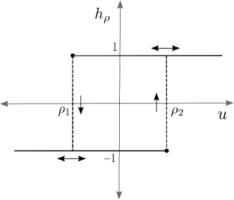
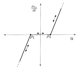
Figure 1: Relay in the $(u,h_{\rho})$-plane for the classical Preisach model (left) and relay slope for the dynamic Preisach model for the case $|\eta_{\rho}|<1$(right). The arrows mark the authorized paths.

Formally, given any couple $\rho=(\rho_{1},\rho_{2})$, such that $\rho_{1}<\rho_{2}$, the corresponding relay operator $h_{\rho}$ is defined as follows: for any $u\in C([0,T])$ and $\xi\in\{1,-1\}$ (an initial condition), $h_{\rho}(u,\xi)$ is a function from $[0,T]$ to $\mathbb{R}$ such that,

$$h_{\rho}(u,\xi)(0):=\left\{\begin{array}[]{rl}-1&\quad\mathrm{if}\;u(0)\leq\rho_{1},\\ \xi&\quad\mathrm{if}\;\rho_{1}<u(0)<\rho_{2},\\ 1&\quad\mathrm{if}\;u(0)\geq\rho_{2}.\\ \end{array}\right.$$

Then, for any $t\in(0,T]$, let us set $X_{u}(t):=\{\tau\in\,(0,t]:\,\,u(\tau)=\rho_{1}\,\,\mbox{or}\,\,\rho_{2}\}$. This set keeps account of the previous instants in which $u$ has got the thresholds $\rho_{1}$ or $\rho_{2}$. We define

$$h_{\rho}(u,\xi)(t):=\left\{\begin{array}[]{cl}h_{\rho}(u,\xi)(0)&\quad\mathrm{if}\,\,X_{u}(t)=\emptyset\,,\\ -1&\quad\mathrm{if}\,\,X_{u}(t)\neq\emptyset\quad\mbox{and}\quad u(\max X_{u}(t))=\rho_{1},\\ ~{}~{}~{}1&\quad\mathrm{if}\,\,X_{u}(t)\neq\emptyset\quad\mbox{and}\quad u(\max X_{u}(t))=\rho_{2}.\\ \end{array}\right.$$ (1)

We notice that $h_{\rho}$ can only be equal to $\pm 1$ depending on the past history of the system, with instantaneous “switch-down” and “switch-up” when $u$ takes the values $\rho_{1}$ and $\rho_{2}$, respectively. The value of the relay operator remains at the last value ($\pm 1$) until $u$ takes the value of one opposite switch, that is, switch to value $1$ when $u$ attains the value $\rho_{2}$ from below, and to $-1$ when it attains $\rho_{1}$ from above.

To define the classical Preisach operator $\mathcal{F}_{{}_{\!\!S}}$, it is useful to introduce the so-called Preisach triangle $\mathcal{T}:=\{\rho=(\rho_{1},\rho_{2})\in\mathbb{R}^{2}:-\rho_{0}\leq\rho_{1}\leq\rho_{2}\leq\rho_{0}\}$ where $\rho_{0}>0$ is given. Let us denote by $Y$ the family of Borel measurable functions ${\mathcal{T}}\rightarrow\{-1,1\}$ and by $\xi$ a generic element of $Y$. Then, $\mathcal{F}_{{}_{\!\!S}}$ is given by:

$$\mathcal{F}_{{}_{\!\!S}}:C([0,T])\times Y\longrightarrow C([0,T]),$$

$$(u,\xi)\longmapsto[\mathcal{F}_{{}_{\!\!S}}(u,\xi)](t)=\int_{\mathcal{T}}[h_{\rho}(u,\xi(\rho))](t)p(\rho)\,d\rho,$$ (2)

where $p\in\mathrm{L}^{1}({\mathcal{T}})$ with $p>0$ is termed Preisach density function. Thus, the classical Preisach model can be understood as the “sum” of a family of static relays, distributed with a certain density $p$. Considering the definition above, this operator is a hysteresis operator in the mathematical sense established by Visintin [41].

Remark 1

If $u=0$ at $t=0$, then we can consider the following initial condition:

$$h_{\rho}(u,\xi)(0):=\left\{\begin{array}[]{cl}-1&\mathrm{if}\,\,\rho_{1}+\rho_{2}>0\\ 1&\mathrm{if}\,\,\rho_{1}+\rho_{2}<0.\\ \end{array}\right.$$ (3)

In electromagnetism, this initial configuration is usually called “demagnetized” or “virginal” state because it leads to a null magnetic induction when $p$ is symmetric [32].

Currently, the classical Preisach model serves as a basis for generalizations that try to overcome some of the lacks of the model. In particular, the fact that the form of the hysteresis diagram does not reflect the frequency content of the input $u(t)$ (see (1) and (2)). In other words, the model is rate-independent [32]; this means that at any instant $t$, $[\mathcal{F}_{{}_{\!\!S}}(u,\xi)](t)$ only depends on the image set $u([0,t])$ and on the order in which these values of $u$ have been attained, but not on the rate of change of $u$. Formally, this can be expressed as follows [41]:

Definition 1

$\zeta:\mbox{Dom}(\zeta)\subset C([0,T])\times[-1,1]$ is said rate independent if the path of the pair $(u,\zeta(u,\xi))$ is invariant with respect to any increasing diffeomorphism $\varphi:[0,T]\rightarrow[0,T]$, i.e.,

$$\forall(u,\xi)\in\mathrm{Dom}(\zeta),$$

$$\zeta(u\circ\varphi,\xi)=\zeta(u,\xi)\circ\varphi~{}~{}\mbox{in}~{}[0,T].$$

In order to take into account the rate-dependent effects, in the following section we will introduce the so-called dynamic relay.

2.2 The dynamic relay

In the rate-dependent generalization of the Preisach model (the so-called dynamic Preisach model) introduced by Bertotti [6, 8], the relays are assumed to switch at a finite rate proportional to the difference between $u(t)$ and the switching values $\rho_{1}$ and $\rho_{2}$ (see Figure 1 (right)). In particular, this means that, contrary to the classical relay where only two states, $-1$ and $1$ are possible, now all intermediate states in the interval $[-1,1]$ can be attained; see Figure 2 and Remark 2. The proportionality factor, denoted by $k$, is a material-dependent parameter.

Formally, for a fixed $\rho=(\rho_{1},\rho_{2})\in\mathbb{R}^{2}$, $\rho_{1}<\rho_{2}$, and motivated by [6], we define the dynamic relay operator $\eta_{\rho}:\mathrm{L}^{2}(0,T)\times[-1,1]\to\mathrm{H}^{1}(0,T)$ such that, for any $u\in\mathrm{L}^{2}(0,T)$ and $\xi\in[-1,1]$, $\eta_{\rho}(u,\xi):[0,T]\to[-1,1]$ is the unique function $y\in\mathrm{H}^{1}(0,T)$ such that $-1\leq y(t)\leq 1$ and solves the nonlinear Cauchy problem:

$$\frac{dy}{dt}(t) =F(t,y(t)):=\left\{\begin{array}[]{l}k(u(t)-\rho_{2})^{+}-k(u(t)-\rho_{1})^{-}\,\,\mbox{ if }-1<y(t)<1,\\ 0\phantom{(u(t)-\rho_{2})}\quad\mbox{ if }y(t)=-1\mbox{ and }u(t)\leq\rho_{2},\\ k(u(t)-\rho_{2})\quad\mbox{ if }y(t)=-1\mbox{ and }u(t)\geq\rho_{2},\\ k(u(t)-\rho_{1})\quad\mbox{ if }y(t)=1\mbox{ and }u(t)\leq\rho_{1},\\ 0\phantom{(u(t)-\rho_{2})}\quad\mbox{ if }y(t)=1\mbox{ and }u(t)\geq\rho_{1},\end{array}\right.$$ (9)

$$y(0) =\xi.$$ (10)

We have used the standard notations:

$$x^{+}=\max\{x,0\}\mbox{ and }x^{-}=\max\{-x,0\},$$

so that $x=x^{+}-x^{-}$. Notice that (9) partially coincides with the definition given in [6] when $-1<y<1$. Nevertheless, in order to perform a suitable mathematical analysis, we need to consider all the other cases included in (9). We also notice that this formulation and that of Bertotti are consistent because cases third and fourth cannot happen, as we will see in the sequel.

Let $g_{\rho}:\mathbb{R}\rightarrow\mathbb{R}$ be defined by

$$g_{\rho}(u):=-k(u-\rho_{1})^{-}+k(u-\rho_{2})^{+}.$$

Then $g$ is Lipschitz-continuous:

$$|g_{\rho}(u_{1})-g_{\rho}(u_{2})|\leq k|u_{1}-u_{2}|.$$

In terms of $g_{\rho}(u(t))$, (9) can be rewritten as follows

$$\frac{dy}{dt}(t) =\left\{\begin{array}[]{ll}g_{\rho}(u(t))&\mbox{ if }-1<y(t)<1,\\ 0&\mbox{ if }y(t)=-1\mbox{ and }g_{\rho}(u(t))\leq 0,\\ g_{\rho}(u(t))&\mbox{ if }y(t)=-1\mbox{ and }g_{\rho}(u(t))\geq 0,\\ g_{\rho}(u(t))&\mbox{ if }y(t)=1\mbox{ and }g_{\rho}(u(t))\leq 0,\\ 0&\mbox{ if }y(t)=1\mbox{ and }g_{\rho}(u(t))\geq 0,\end{array}\right.$$ (16)

$$y(0) =\xi,$$ (17)

To prove the existence and uniqueness of such a function $y$ we will consider another apparently different initial-value problem, namely, find $y\in\mathrm{H}^{1}(0,T)$ satisfying $-1\leq y(t)\leq 1$ and $q\in\mathrm{L}^{2}(0,T)$ such that

$$\left\{\begin{array}[]{l}\dfrac{dy}{dt}(t)=g_{\rho}(u(t))-q(t),\\ y(0)=\xi,\end{array}\right.$$ (18)

and

$$\left\{\begin{array}[]{ll}q(t)=0&\mbox{ if }|y(t)|<1,\\ q(t)\in(-\infty,0]&\mbox{ if }y(t)=-1,\\ q(t)\in[0,\infty)&\mbox{ if }y(t)=1.\end{array}\right.$$ (19)

Function $q(t)$ is a priori unknown and can be considered as a Lagrange multiplier associated with the constraint $|y(t)|\leq 1$. In fact, problem (18)-(19) can be written in a more compact but equivalent way as a multi-valued ordinary differential equation:

$$\left\{\begin{array}[]{l}\dfrac{dy}{dt}(t)+\partial\chi_{[-1,1]}(y(t))\ni g_{\rho}(u(t)),\\ y(0)=\xi,\end{array}\right.$$ (20)

where $\partial\chi_{[-1,1]}$ denotes the sub-differential of $\chi_{[-1,1]}$ which is the indicator function of the interval $[-1,1]$. Let us recall that (see, for instance, [10])

$$\chi_{[-1,1]}(x)=\left\{\begin{array}[]{ll}\infty&\mbox{ if }|x|>1,\\ 0&\mbox{ if }|x|\leq 1,\end{array}\right.\qquad\mbox{and}\qquad\partial\chi_{[-1,1]}(x)=\left\{\begin{array}[]{ll}[0,\infty)&\mbox{ if }x=1,\\ (-\infty,0]&\mbox{ if }x=-1,\\ 0&\mbox{ if }|x|<1,\\ \emptyset&\mbox{ if }|x|>1.\end{array}\right.$$

Thus, it is easy to see that function $q(t)$ belongs to $\partial\chi_{[-1,1]}(y(t))$ for each $t\in[0,T]$ which means $|y(t)|\leq 1$ and

$$q(t)\Big{(}z-y(t)\Big{)}\leq 0\quad\forall z\in\mathbb{R}\mbox{ with }|z|\leq 1.$$

Indeed, we notice that the latter is equivalent to (19). Let us emphasize that function $q(t)$ is also an unknown of the problem and, as we will see below, it is unique too. Actually, the value of $q(t)$ accommodates so that the solution of the Cauchy problem satisfies $|y(t)|\leq 1$, i.e., it is a Lagrange multiplier associated to this constraint.

The existence of a unique solution to the Cauchy problem (20) has been proved in a much more general setting (see for instance [10]). However, for the sake of completeness we include a direct proof for this simpler case in A.

Theorem 2.1

Let us assume that $u$ is a given function in $\mathrm{L}^{2}(0,T)$. Then for each $\xi\in[-1,1]$ there exists a unique function $y\in\mathrm{H}^{1}(0,T)$ satisfying (20). Consequently, function $q(t)$ defined almost everywhere by

$$q(t):=-\dfrac{dy}{dt}(t)-k(u(t)-\rho_{1})^{-}+k(u(t)-\rho_{2})^{+}$$

belongs to $\mathrm{L}^{2}(0,T)$ and $q(t)\in\partial\chi_{[-1,1]}(y(t))\mbox{ a.e. in }(0,T)$.

We also have the following characterization of $q(t)$.

Lemma 2.2

For a.e. in $[0,T]$ we have,

$$q(t)=P_{\partial\chi_{[-1,1]}(y(t))}\big{(}g_{\rho}(u(t))\big{)}=\left\{\begin{array}[]{ll}0&\mbox{ if }-1<y(t)<1,\\ g_{\rho}(u(t))&\mbox{ if }y(t)=-1\mbox{ and }g_{\rho}(u(t))\leq 0,\\ 0&\mbox{ if }y(t)=-1\mbox{ and }g_{\rho}(u(t))\geq 0,\\ 0&\mbox{ if }y(t)=1\mbox{ and }g_{\rho}(u(t))\leq 0,\\ g_{\rho}(u(t))&\mbox{ if }y(t)=1\mbox{ and }g_{\rho}(u(t))\geq 0,\end{array}\right.$$ (21)

where $P_{\partial\chi_{[-1,1]}(y(t))}$ denotes the projection on the set $\partial\chi_{[-1,1]}(y(t))$.

Proof 1

It follows immediately from Remark 3.9 in [10].

As a consequence of the previous characterization of $q(t)$ we obtain an equivalent expression for (18).

Corollary 2.3

We have, a.e. in $[0,T]$,

$$\frac{dy}{dt}(t)=g_{\rho}(u(t))-q(t)=\left\{\begin{array}[]{ll}g_{\rho}(u(t))&\mbox{ if }-1<y(t)<1,\\ 0&\mbox{ if }y(t)=-1\mbox{ and }g_{\rho}(u(t))\leq 0,\\ g_{\rho}(u(t))&\mbox{ if }y(t)=-1\mbox{ and }g_{\rho}(u(t))\geq 0,\\ g_{\rho}(u(t))&\mbox{ if }y(t)=1\mbox{ and }g_{\rho}(u(t))\leq 0,\\ 0&\mbox{ if }y(t)=1\mbox{ and }g_{\rho}(u(t))\geq 0.\end{array}\right.$$ (22)

and, therefore, the solution of (20) is also the solution of the original problem (9)-(10). This follows from (22) and the fact that $g_{\rho}(u(t))\leq 0$ is equivalent to $u(t)\leq\rho_{2}$, and the same is true for $g_{\rho}(u(t))\geq 0$ and $u(t)\geq\rho_{1}$.

From the previous analysis it follows that, for a given input $u$ and initial state $\xi$, the dynamic relay can be computed by solving the multi-valued ordinary differential equation (20). This can be done, for instance, by using semi-smooth Newton [21] or Bermúdez-Moreno method [5], just to name a few. However, motivated by [6], we notice that for an input $u\in C([0,T])$ such that $X_{u}(T)=\{t_{u}^{1},\ldots,t_{u}^{M}\},M\geq 1$, if we define $t_{u}^{0}:=0$ and $t_{u}^{M+1}:=T$, then the dynamic relay $y:=\eta_{\rho}(u,\xi)$ can be obtained by integrating (22) (equivalently (9)) with respect to $t$ and taking into account the saturation $-1\leq y\leq 1$. Notice that, for each $t\in(t_{u}^{m},t_{u}^{m+1}],m=0,\ldots,M+1$, $y(t)$ is either nondecreasing (if $u(t)\geq\rho_{2}$), or nonincreasing (if $u(t)\leq\rho_{1}$) or constant (if $\rho_{1}\leq u(t)\leq\rho_{2}$). For ease of presentation, in order to obtain an expression for $y(t)$, we consider the first interval, namely, $t\in(t_{u}^{0},t_{u}^{1}]$. In this case it follows that,

• If $\rho_{1}\leq u(t)\leq\rho_{2}$ then, from (22), the slope of $y$ vanishes along the interval. Thus, $y(t)=y(t_{u}^{0})=\xi$ on $(t_{u}^{0},t_{u}^{1}]$.

• If $u(t)\geq\rho_{2}$ then $y(t)$ increases but cannot exceed $1$. Notice that the third case in (22) cannot be fulfilled on $(t_{u}^{0},t_{u}^{1}]$, because, when $y(t_{u}^{0})=-1$ the slope of $y$ is positive and $y(t)>-1,t\in(t_{u}^{0},t_{u}^{1}]$ . Thus, If $|y|<1$ or $y=1$, from the first and fifth cases in (22), respectively, we arrive at

  $$y(t)=\min\left\{1,y(t_{u}^{0})+\displaystyle\int_{t_{u}^{0}}^{t}k(u(s)-\rho_{2})ds\right\}.$$

• If $u(t)\leq\rho_{1}$, then $y(t)$ decreases but cannot be less than $-1$. Similar to the previous case, we notice that the fourth case in (22) cannot be fulfilled on $(t_{u}^{0},t_{u}^{1}]$ because when $y(t_{u}^{0})=1$ the slope of $y$ is negative and $y(t)<1,t\in(t_{u}^{0},t_{u}^{1}].$ Thus, if $|y|<1$ or $y=-1$, from the first and second cases in (22), respectively, we arrive at

  $$y(t)=\max\left\{-1,y(t_{u}^{0})+\displaystyle\int_{t_{u}^{0}}^{t}k(u(s)-\rho_{1})ds\right\}.$$

Thus, by proceeding similarly with the remaining intervals, it follows that for $t\in~{}(t_{u}^{m},t_{u}^{m+1}],m=0,\ldots,M$:

$$y(t) =\left\{\begin{array}[]{cl}\min\left\{1,y(t_{u}^{m})+\displaystyle\int_{t_{u}^{m}}^{t}k(u(s)-\rho_{2})ds\right\}&\mbox{ if }u(s)\geq\rho_{2}\mbox{ for }s\in(t_{u}^{m},t],\\ \max\left\{-1,y(t_{u}^{m})+\displaystyle\int_{t_{u}^{m}}^{t}k(u(s)-\rho_{1})ds\right\}&\mbox{ if }u(s)\leq\rho_{1}\mbox{ for }s\in(t_{u}^{m},t],\\ y(t_{u}^{m})&\mbox{otherwise.}\end{array}\right.$$ (26)

To give an idea of the plane curve $t\in[0,T]\rightarrow(u(t),y(t))$, we consider two examples with a sinusoidal input $u(t)=200\sin(2\pi ft)$ and initial condition $\xi=-1$. This input is depicted in Figure 2 (top and bottom left) for frequency $f=20$Hz, where the dotted lines represent different $(\rho_{1},\rho_{2})$ values. Figure 2 (top right) shows the curve $t\in[0,T]\rightarrow(u(t),y(t))$ when the relay $\eta_{\rho}$ is characterized by switching values $(\rho_{1},\rho_{2})=(50,100)$ and slopes $k\in\{1,50,10^{8}\}$. For the same slopes, in Figure 2 (bottom right) we show this curve for switching values $(\rho_{1},\rho_{2})=(-50,50)$. Notice that $(u(t),y(t))$ may vary in an asymmetric way when the input is not symmetric with respect to $(\rho_{1},\rho_{2})$ (see dashed line in Figure 2 (top right)). We also notice that the dash-dotted line in Figure 2 (top and bottom right) becomes similar to the discontinuous relay of the classical Preisach model (see Figure 1 (left)), that is, the classical relay can be seen as the limit as $k\rightarrow\infty$ of the dynamic relay.

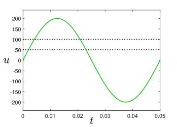
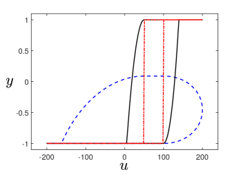
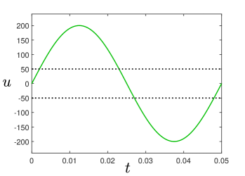
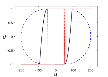
Figure 2: Input function $u(t)=200\sin(2\pi ft)$ (left) for frequency $f=20$Hz. Three dynamic relays are presented for switching values $(\rho_{1},\rho_{2})=(50,100)$ (top), $(\rho_{1},\rho_{2})=(-50,50)$ (bottom) and initial state $\xi=-1$. The switching values are represented by dotted lines on the left panels. The right panels show the different relay with slopes $k=1$ (dashed line), $k=50$ (solid line) and $k=10^{8}$ (dash-dotted line).

For the second example we analyze the evolution of the relays with a sinusoidal input $u(t)=200\sin(2\pi ft)$ for $k=50$ and different frequencies $f$. Figure 3 shows the dynamic relays characterized by $(\rho_{1},\rho_{2})=(50,100)$ (top right) and $(\rho_{1},\rho_{2})=(-50,50)$ (bottom right) for frequencies 50, 500 and 5000 Hz. From these examples we can see the variation of the dynamic relay with respect to $k$ and the input rate. In particular, Figure 3 shows that the dynamic relay is rate-dependent.

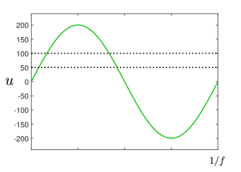
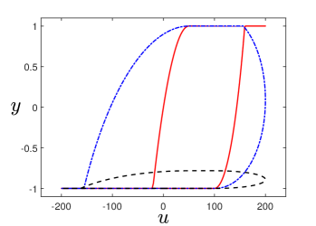
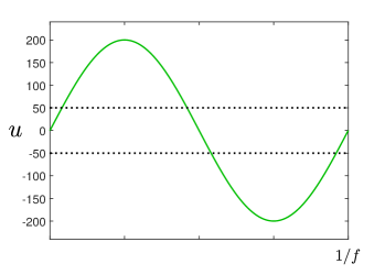
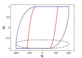
Figure 3: Input function $u(t)=200\sin(2\pi ft)$ (left) for a fixed frequency denoted by $f$. Three dynamic relays are presented for switching values $(\rho_{1},\rho_{2})=(50,100)$ (top), $(\rho_{1},\rho_{2})=(-50,50)$ (bottom) and initial state $\xi=-1$. The switching values are represented by dotted lines on the left panels. The figures at the right show the $(u,y)$ curve corresponding to the dynamic relay for $k=50$ and three frequencies: $f=50$Hz (dashed line), $f=500$Hz (dash-dotted line) and $f=5000$Hz (solid line).

Remark 2

Unlike the classical Preisach model, in the dynamic model the initial state $\xi$ belongs to $[-1,1]$ instead of $\{-1,1\}$. Figure 4 shows the relays for $u_{1}(t)=150\sin(2\pi ft)$ and $u_{2}(t)=150\sin(2\pi ft)+75$, for $f=20$ Hz and two different initial states: $\xi_{1}=-0.5$ (left) and $\xi_{2}=0.5$ (right). Two slopes are considered for each initial state: $k=5$ and $k=50$.

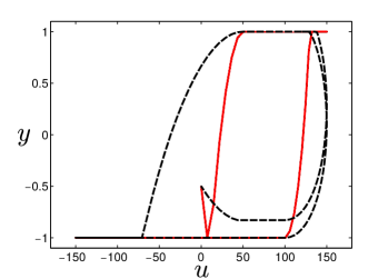
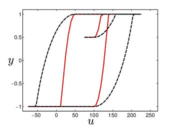
Figure 4: The left panel shows a dynamic relay corresponding to the input $u_{1}(t)=150\sin(2\pi ft)$ and initial state $\xi=-0.5$. The right panel shows a dynamic relay corresponding to input $u_{2}(t)=150\sin(2\pi ft)+75$ and initial state $\xi=0.5$. For both relays $f=20$ Hz; two slopes, $k=50$ (solid line) and $k=5$ (dashed line) are considered.

From the previous examples we notice that, unlike the classical static relay, the dynamic relay $\eta_{\rho}$ does not satisfy either the so-called rate independence (see Definition 1) or the piecewise monotonicity properties defined as follows:

Definition 2

$\zeta$ is said piecewise monotone if when $u$ is either nondecreasing or nonincreasing in $[t_{1},t_{2}]\subset[0,T]$ then so is $\zeta(u,\xi)(t)$.

Notice that the dashed curve on Figure 3 (right) shows that the latter is not satisfied by the dynamic relay.

In the sequel we will show some properties of the dynamic relay solution to (9)-(10). The following lemma shows that, like the classical relay, the dynamic relays “preserves the order” of the inputs.

Lemma 2.4

Let $u_{1},u_{2}\in\mathrm{L}^{2}(0,T)$, $\xi_{1},\xi_{2}\in[-1,1]$ and $k>0$. The dynamic relay $\eta_{\rho}$ satisfies the following order preservation property:

$$\mbox{If }u_{1}\leq u_{2}\mbox{ a.e. in }[0,T]\mbox{ and }\xi_{1}\leq\xi_{2},\mbox{ then }[\eta_{\rho}(u_{1},\xi_{1})](t)\leq[\eta_{\rho}(u_{2},\xi_{2})](t)\,\,\forall t\in[0,T].$$ (27)

Proof 2

Let $y_{i}(t)$ be the solution of problem (20) for $u=u_{i}(t)$, $i=1,2$ and respective initial condition $y_{i}(0)=\xi_{i}$, $i=1,2$. Then we have

$$\frac{dy_{1}}{dt}-\frac{dy_{2}}{dt}+q_{1}(t)-q_{2}(t)=g_{\rho}(u_{1}(t))-g_{\rho}(u_{2}(t)),$$ (28)

$y_{1}(0)-y_{2}(0)=\xi_{1}-\xi_{2}$ and $q_{i}(t)\in\partial\chi_{[-1,1]}(y_{i}(t))$, $i=1,2$. Let us multiply (28) by $\big{(}y_{1}(t)-y_{2}(t)\big{)}^{+}$. We get

$$\frac{1}{2}\frac{d}{dt}|\big{(}y_{1}(t)-y_{2}(t)\big{)}^{+}|^{2}+(q_{1}(t)-q_{2}(t))\big{(}y_{1}(t)-y_{2}(t)\big{)}^{+}\\ =\big{(}g_{\rho}(u_{1}(t))-g_{\rho}(u_{2}(t))\big{)}(y_{1}(t)-y_{2}(t)\big{)}^{+}\leq 0$$

By integrating from $0$ to $T$ and using the monotonicity of $\partial\chi_{[-1,1]}$ we deduce

$$\frac{1}{2}|\big{(}y_{1}(t)-y_{2}(t)\big{)}^{+}|^{2}\leq\frac{1}{2}|\big{(}y_{1}(0)-y_{2}(0)\big{)}^{+}|^{2}=\frac{1}{2}|\big{(}\xi_{1}-\xi_{2}\big{)}^{+}|^{2}=0$$

Hence $\big{(}y_{1}(t)-y_{2}(t)\big{)}^{+}=0$ from which the result follows.

As a consequence of the previous result, the following property, to be used in the sequel, holds true.

Corollary 2.5

Let $\xi\in[-1,1]$ and $u,v\in\mathrm{L}^{2}(0,T)$ such that $u(t)=v(t)$ a.e. in $[0,t_{1}]$. If $u\geq v$ a.e. in $[t_{1},t_{2}]$, $t_{1}\leq t_{2}$, then

$$\left([\eta_{\rho}(u,\xi)](t)-[\eta_{\rho}(v,\xi)](t)\right)\left(u(t)-v(t)\right)\geq 0\mbox{ a.e. in }[t_{1},t_{2}].$$ (29)

The following lemma establishes a continuity property of dynamic relays.

Lemma 2.6

Let $k>0$ be given, then the operator $\eta_{\rho}:\mathrm{L}^{2}(0,T)\times[-1,1]\to C([0,T])$ is Lipschitz-continuous. More precisely, let $u_{1},\,u_{2}$ be any functions in $\mathrm{L}^{2}(0,T)$, $\xi_{1},\xi_{2}\in[-1,1]$, and $y_{1},\,y_{2}$ their respective solutions of the Cauchy problem (20). Then we have

$$\|y_{1}-y_{2}\|_{C([0,T])}\leq\mathrm{e}^{\frac{T}{2}}\Big{(}|\xi_{1}-\xi_{2}|+k\|u_{1}-u_{2}\|_{\mathrm{L}^{2}(0,T)}\Big{)}.$$ (30)

Proof 3

Let us denote by $y_{1}(t)$ and $y_{2}(t)$ the solutions of (20) corresponding to functions $u_{1}$, $u_{2}$ in $\mathrm{L}^{2}(0,T)$ and initial conditions $\xi_{1}$ and $\xi_{2}$, respectively. Then there must exist $q_{i}(t)\in\partial\chi_{[-1,1]}(y_{i}(t)),\ i=1,2$ such that

$$\dfrac{dy_{i}}{dt}(t)+q_{i}(t)=g_{\rho}(u_{i}(t)),\ i=1,2.$$

Let us subtract the above equations for $i=1,2$ and then make the scalar product by $y_{1}-y_{2}$. We get

$$\frac{1}{2}\frac{d}{dt}|y_{1}(t)-y_{2}(t)|^{2}\leq|g_{\rho}(u_{1}(t))-g_{\rho}(u_{2}(t))|\,|y_{1}(t)-y_{2}(t)|$$

because $(q_{1}(t)-q_{2}(t))(y_{1}(t)-y_{2}(t))\geq 0,$ as $\partial\chi_{[-1,1]}$ is monotone. By integrating from $0$ to $t$ we obtain

$$\frac{1}{2}|y_{1}(t)-y_{2}(t)|^{2}\leq\frac{1}{2}|\xi_{1}-\xi_{2}|^{2}+\int_{0}^{t}|g_{\rho}(u_{1}(s))-g_{\rho}(u_{2}(s))|\,|y_{1}(s)-y_{2}(s)|\;ds$$

$$\leq\frac{1}{2}|\xi_{1}-\xi_{2}|^{2}+\left(\int_{0}^{t}|g_{\rho}(u_{1}(s))-g_{\rho}(u_{2}(s))|^{2}\;ds\right)^{1/2}\,\left(\int_{0}^{t}|y_{1}(s)-y_{2}(s)|^{2}\;ds\right)^{1/2}$$

$$\leq\frac{1}{2}|\xi_{1}-\xi_{2}|^{2}+\frac{1}{2}\int_{0}^{t}|g_{\rho}(u_{1}(s))-g_{\rho}(u_{2}(s))|^{2}\;ds+\frac{1}{2}\int_{0}^{t}|y_{1}(s)-y_{2}(s)|^{2}\;ds$$

and then

$$|y_{1}(t)-y_{2}(t)|^{2}\leq|\xi_{1}-\xi_{2}|^{2}+k^{2}\int_{0}^{t}|u_{1}(s)-u_{2}(s)|^{2}\;ds+\int_{0}^{t}|y_{1}(s)-y_{2}(s)|^{2}\;ds.$$

By using the generalized Gronwall’s inequality (see, for instance, Lemma 6.2 in [19]) we deduce

$$|y_{1}(t)-y_{2}(t)|^{2}\leq\,\mathrm{e}^{t}\left(|\xi_{1}-\xi_{2}|^{2}+k^{2}\int_{0}^{t}|u_{1}(s)-u_{2}(s)|^{2}\;ds\right)$$

and finally

$$\max_{t\in[0,T]}|y_{1}(t)-y_{2}(t)|\leq\mathrm{e}^{\frac{T}{2}}\left(|\xi_{1}-\xi_{2}|^{2}+k^{2}\int_{0}^{T}|u_{1}(s)-u_{2}(s)|^{2}\;ds\right)^{\frac{1}{2}}$$

$$\leq\mathrm{e}^{\frac{T}{2}}\left(|\xi_{1}-\xi_{2}|+k\Big{(}\int_{0}^{T}|u_{1}(s)-u_{2}(s)|^{2}\;ds\Big{)}^{\frac{1}{2}}\right)$$

which finishes the proof.

3 Dynamic Preisach model

In this section we introduce the dynamic Preisach operator and prove some properties which are similar to the ones satisfied by the classical Preisach operator. Given $\rho_{0}>0$, let us consider again the Preisach triangle $\mathcal{T}:=\{\rho=(\rho_{1},\rho_{2})\in\mathbb{R}^{2}:-\rho_{0}\leq\rho_{1}\leq\rho_{2}\leq\rho_{0}\}$ (see Figure 5 (left)) and the Preisach function $p\in\mathrm{L}^{1}(\mathcal{T})$ with $p>0$. We denote by $Y$ the convex set of initial configurations which can be defined by

$$Y:=\left\{v\in L^{1}_{p}(\mathcal{T}):|v(\rho)|\leq 1,\mbox{ a.e. }\rho\in\mathcal{T}\right\}$$

where

$$L^{1}_{p}(\mathcal{T}):=\{\xi:\mathcal{T}\to\mathbb{R}\mbox{ Lebesgue-measurable such that }\int_{\mathcal{T}}|\xi(\rho)|p(\rho)\,d\rho<\infty\}$$

endowed with the norm

$$\|\xi\|_{L^{1}_{p}(\mathcal{T})}:=\int_{\mathcal{T}}|\xi(\rho)|p(\rho)\,d\rho.$$

Let us define the dynamic Preisach operator (see [6])

$$\mathcal{F}_{{}_{\!\!D}}:\mathrm{L}^{2}(0,T)\times Y\longrightarrow\mathrm{H}^{1}(0,T),$$

$$(u,\xi)\longmapsto[\mathcal{F}_{{}_{\!\!D}}(u,\xi)](t)=\int_{\mathcal{T}}[\eta_{\rho}(u,\xi(\rho))](t)p(\rho)\,d\rho,$$ (31)

Notice that, if $\eta_{\rho}$ is replaced by $h_{\rho}$ given by (1) then we obtain the classical, rate-independent, Preisach model.

Mathematical properties of the classical Preisach operator are well known (see, for instance, [41]) but this is not the case for the dynamic model. From Lemmas 2.4 and 2.6 we obtain the following properties of the dynamic Preisach model.

Lemma 3.1

The dynamic Preisach operator $\mathcal{F}_{{}_{\!\!D}}:\mathrm{L}^{2}(0,T)\times Y\longrightarrow\mathrm{H}^{1}(0,T)$ is order preserving $(\textrm{cf}.~{}\eqref{eq:order_pre})$ and satisfies the following properties:

• It is Lipschitz-continuous; more precisely, for all $u_{1},u_{2}\in\mathrm{L}^{2}(0,T)$ and $\xi_{1},\xi_{2}\in Y$,

  $$\|\mathcal{F}_{{}_{\!\!D}}(u_{1},\xi_{1})-\mathcal{F}_{{}_{\!\!D}}(u_{2},\xi_{2})\|_{C([0,T])}\\ \leq\mathrm{e}^{\frac{T}{2}}\left(\|\xi_{1}-\xi_{2}\|_{L^{1}_{p}(\mathcal{T})}+k\|u_{1}-u_{2}\|_{\mathrm{L}^{2}(0,T)}\int_{\mathcal{T}}p(\rho)\,d\rho\right).$$

• It is bounded in the following sense: for all $v\in\mathrm{L}^{2}(0,T)$ and $\xi\in Y$,

  $$\left\|\mathcal{F}_{{}_{\!\!D}}(v,\xi)\right\|_{C([0,T])}\leq\displaystyle\int_{\mathcal{T}}p(\rho)\,d\rho.$$ (32)

Proof 4

The order preserving property is a consequence of Lemma 2.4 and the positivity of the Preisach function $p$.

The Lipschitz-continuity follows from Lemma 2.6. Indeed, we have

$$\|\mathcal{F}_{{}_{\!\!D}}(u_{1},\xi_{1})-\mathcal{F}_{{}_{\!\!D}}(u_{2},\xi_{2})\|_{C[0,T]} \leq\int_{\mathcal{T}}\max_{t\in[0,T]}\left\{|[\eta_{\rho}(u_{1},\xi_{1}(\rho))](t)-[\eta_{\rho}(u_{2},\xi_{2}(\rho))](t)|\right\}p(\rho)\,d\rho$$

$$\leq\mathrm{e}^{\frac{T}{2}}\left(\int_{\mathcal{T}}|\xi_{1}(\rho)-\xi_{2}(\rho)|p(\rho)\,d\rho+k\|u_{1}-u_{2}\|_{\mathrm{L}^{2}(0,T)}\int_{\mathcal{T}}p(\rho)\,d\rho\right),$$

from which the result follows.

Finally (32) is a consequence of the fact that $|\eta_{\rho}(u,\xi(\rho))(t)|\leq 1\ \forall t\in[0,T].$

As mentioned, in the classical Preisach model the relay $h_{\rho}$ only takes values $+1$ or $-1$. Thus, at each time $t\geq t^{0}$, the Preisach triangle $\mathcal{T}$ is subdivided into two sets (one possibly empty):

$$S_{u}^{-}(t):=\left\{(\rho_{1},\rho_{2})\in\mathcal{T}:[h_{\rho}(u,\xi)](t)=-1\right\},\,S_{u}^{+}(t):=\left\{(\rho_{1},\rho_{2})\in\mathcal{T}:[h_{\rho}(u,\xi)](t)=1\right\},$$

and consequently

$$[\mathcal{F}_{{}_{\!\!S}}(u,\xi)](t)=\int_{S_{u}^{+}(t)}p(\rho)\,d\rho-\int_{S_{u}^{-}(t)}p(\rho)\,d\rho.$$

However, this is not the case for the dynamic model where the relays vary at finite rate between $-1$ and $1$. Figure 6 shows the classical and dynamic relay configuration with respect to the same input $u$ depicted in Figure 6 (top left). For this example we have considered a Preisach triangle characterized by $\rho_{0}=300$, a constant $k=50$ and the demagnetized state as initial condition (cf. (1)).

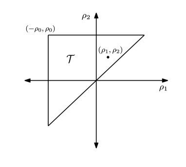
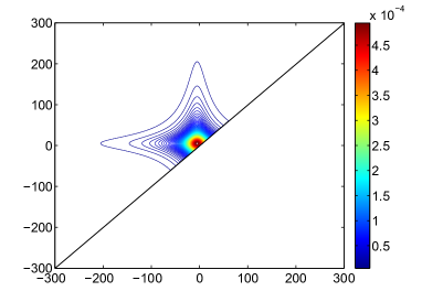
Figure 5: Preisach triangle (left) and Factorized-Lorentzian distribution $p$ (right) with $N=1/2000$, $\omega=5$ and $\gamma=4$.

We also compute the dynamic Preisach operator $\mathcal{F}_{{}_{\!\!D}}(u,\xi)$ for $u$ depicted in Figure 6 (top left) for different $k$ values and frequencies. For the dynamic relay we have considered $k=50$ and the Preisach function $p$ is given by the Factorized-Lorentzian distribution [7] (see Figure 5 (right)):

$$p(\rho_{1},\rho_{2}):=N\left(1+\left(\dfrac{\rho_{2}-\omega}{\gamma\omega}\right)^{2}\right)^{-1}\left(1+\left(\dfrac{\rho_{1}+\omega}{\gamma\omega}\right)^{2}\right)^{-1}$$ (33)

with $N=1/2000$, $\omega=5$ and $\gamma=4$. Figure 7 shows the dynamic curve $(u,\mathcal{F}_{{}_{\!\!D}}(u,\xi))$ for different $k$ values and input velocities.

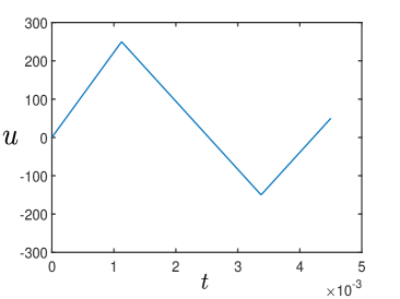
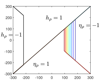
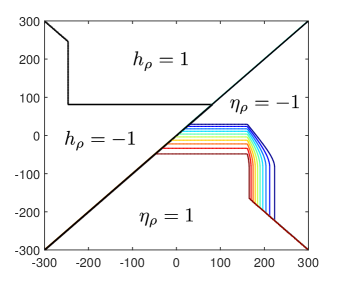
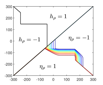
Figure 6: Input function $u(t)$ (top left) defined in $[0,0.0045]$. The isolines represent the corresponding dynamic relay values $\eta_{\rho}$ for $k=50$ and the classical relay $h_{\rho}$ at $t=0.001$ (top right), $t=0.003$ (bottom left) and t= 0.0045 (bottom right). For compactness we have considered the dynamic and classical relay in the same figure.

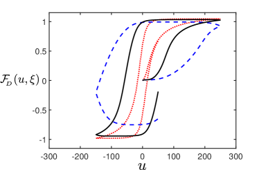
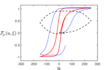
Figure 7: Dynamic Preisach hysteresis curve $\mathcal{F}_{{}_{\!\!D}}$ for a Factorized-Lorentzian distribution, diferent $k$ values and input $u(t)$ depicted on Figure 6 (top left). Left: input $u$ defined in $[0,0.0045]$ and slope values $k=25$ (dashed line), $k=200$ (solid line) and $k=10^{8}$ (dotted line). Right: slope value $k=100$ and input function $u(t)$ defined in $[0,4.5]$ (solid line), $[0,0.0045]$ (dotted line) and $[0,0.00045]$ (dashed line).

Finally, since we are interested in the mathematical analysis and computation of distributed electromagnetic models (also called field models), following [41] we introduce a space-time dependent operator. Given a time dependent input field $u(x,\cdot)\in\mathrm{L}^{2}(0,T)$ and an initial state field $\xi(x)\in Y,$ we define a space and time dependent hysteresis operator $\mathcal{F}:\mathrm{L}^{2}(0,T;\mathrm{L}^{2}(\Omega))\times\mathrm{L}^{2}(\Omega;Y)\to C(0,T;\mathrm{L}^{2}(\Omega))$ as follows:

$$[\mathcal{F}(u,\xi)](x,t):=[\mathcal{F}_{{}_{\!\!D}}(u(x,\cdot),\xi(x))](t)\quad,\mbox{ a.e. in }[0,T]\times\Omega$$ (34)

where $\mathrm{L}^{2}(\Omega;Y)$ is a subset of $\mathrm{L}^{2}(\Omega;\mathrm{L}^{1}_{p}(\mathcal{T}))$, the space of all function $v:\Omega\to\mathrm{L}^{1}_{p}(\mathcal{T})$ such that

$$\left\|v\right\|_{\mathrm{L}^{2}(\Omega;\mathrm{L}^{1}_{p}(\mathcal{T}))}:=\left(\int_{\Omega}\left\|u\right\|_{\mathrm{L}^{1}_{p}(\mathcal{T})}^{2}\right)^{1/2}<\infty.$$

Let us emphasize that operator $\mathcal{F}$ is local in $x$ but non-local in $t$. We end this section with the following properties of dynamic operator $\mathcal{F}$ which follow from Lemma 3.1.

Lemma 3.2

The dynamic Preisach operator $\mathcal{F}:\mathrm{L}^{2}(0,T;\mathrm{L}^{2}(\Omega))\times\mathrm{L}^{2}(\Omega;Y)\to C(0,T;\mathrm{L}^{2}(\Omega))$ is uniformly bounded, order preserving $(\textrm{cf}.~{}\eqref{eq:order_pre})$ and Lipschitz-continuous in the following sense: there exists $C$ depending on $k$ such that, for all $u_{1},u_{2}\in\mathrm{L}^{2}(0,T;\mathrm{L}^{2}(\Omega))$ and $\xi_{1},\xi_{2}\in\mathrm{L}^{2}(\Omega;Y)$

$$\|\mathcal{F}(u_{1},\xi_{1})-\mathcal{F}(u_{2},\xi_{2})\|_{C(0,T;\mathrm{L}^{2}(\Omega)))}\leq C\left(\left\|\xi_{1}-\xi_{2}\right\|_{\mathrm{L}^{2}(\Omega;\mathrm{L}^{1}_{p}(\mathcal{T}))}+\left\|u_{1}-u_{2}\right\|_{\mathrm{L}^{2}(0,T;\mathrm{L}^{2}(\Omega))}\right).$$

4 Parabolic problem with dynamic hysteresis

In this section we introduce a parabolic problem with dynamic hysteresis for which we state an existence result by using the properties proved on the previous section.

Let $T>0$ and $\Omega\in\mathbb{R}^{d},d=2,3$ be a bounded domain with smooth boundary $\Gamma=\partial\Omega$. Let $V\subset H$ be two Hilbert spaces of scalar functions defined in $\Omega$ with continuous, dense, compact embedding. Then we have $V\subset H\equiv H^{\prime}\subset V^{\prime}$. We consider a mapping $a:(0,T)\times V\times V\to\mathbb{R}$ such that $a(t,\cdot,\cdot)$ is bilinear a.e. $t\in(0,T)$. We are interested in the mathematical analysis of the following parabolic problem: find $u\in\mathrm{L}^{2}(0,T;V)\cap\mathrm{L}^{\infty}(0,T;H)$ with $\partial_{t}u\in\mathrm{L}^{2}(0,T;V^{\prime})$ and $w\in\mathrm{L}^{2}(0,T;H)$ with $\partial_{t}w\in\mathrm{L}^{2}(0,T;V^{\prime})$, such that

$$\left\langle\partial_{t}u+\partial_{t}w,v\right\rangle_{V,V^{\prime}}+a(t,u,v) =\langle f,v\rangle_{V,V^{\prime}}\quad\forall v\in V,\quad\mbox{a.e. in }(0,T],$$ (35a)

$$w =\mathcal{F}(u,\xi)\qquad\mbox{in }\Omega\times[0,T],$$ (35b)

$$(u+w)(0) =u_{0}+w_{0}\,\,\,\,\quad\mbox{in }\Omega.$$ (35c)

Here, operator $\mathcal{F}$ is defined by (34). We introduce the following assumptions that will be used to prove the existence of a solution to (35):

• $a(\cdot,u,v)$ is a continuous form in $V\times V$. Moreover, it is Lipschitz continuous in $t$ and satisfies the Gårding’s inequality

  $$a(t,v,v)+\lambda\|G\|_{{H}}^{2}\geq\gamma\|G\|_{V}^{2}\quad\forall v\in V,\quad\forall t\in[0,T],$$ (36)

  for some constants $\lambda,\gamma\geq 0$.

• $f$ belongs to $\mathrm{H}^{1}(0,T;V^{\prime})$, $u_{0}\in V$ and $w_{0}:=\mathcal{F}(u_{0})\in H$.

• For a fixed initial state $\xi:\Omega\to Y$, the mapping $\mathcal{F}:\mathrm{L}^{2}(0,T;H)\to C(0,T;H)$ is well defined and Lipschitz continuous in the following sense: there exits $C>0$ such that:

  $$\|\mathcal{F}(u,\xi)-\mathcal{F}(v,\xi)\|_{C(0,T;H))}\leq C\left\|u-v\right\|_{\mathrm{L}^{2}(0,T;H)}.$$

The next result shows the existence of solution to problem (35). The proof is carried out through three different steps: time discretization, a priori estimates and passage to the limit by using compactness (cf. H.3). This approximation procedure is often used in the analysis of equations that include a memory operator since at any time-step we solve a stationary problem in which this operator is reduced to a standard nonlinear mapping (see, for instance, [41]).

Theorem 4.1

Let us assume H.1, H.2 and H.3 hold true. Then, problem (35) has a solution.

Proof 5

Let us fix $m\in\mathbb{N}$ and set $\Delta t:=T/m$. Now, for $n=1,\ldots,m$, we define $t^{n}:=n\Delta t$. The time discretization of problem (35) based on backward Euler’s scheme reads as follows: Given $u^{0}=u_{0}$ and $w^{0}=w_{0}$ in $\Omega$, find $u^{n}\in V$ and $w^{n}\in H$, $n=1,\ldots,m$, satisfying

$$\left(u^{n}+w^{n},v\right)_{H,H}+\Delta ta(t^{n},u^{n},v) =\Delta t\langle f^{n},v\rangle_{V,V^{\prime}}+(u^{n-1}+w^{n-1},v),$$ (37)

$$w^{n} =[\mathcal{F}(u_{\Delta t^{n}},\xi)](t^{n})\qquad\quad\mbox{in }\Omega,$$ (38)

for all $v\in V$, where $u_{\Delta t^{n}}$ is the piecewise linear in time interpolant of $\{u^{i}\}_{i=0}^{n}$. In order to study the time-discrete problem we introduce an operator $F^{n}:H\longrightarrow H$ as follows:

$$F^{n}(w):=[\mathcal{F}(\Lambda^{n}(w),\xi)](t^{n})\quad\forall w\in H,$$

where $\Lambda^{n}:H\rightarrow\mathrm{H}^{1}(0,t^{n};H)$ is defined as follows: for $w\in H$, $\Lambda^{n}(w)$ is the continuous piecewise linear function in time such that $\Lambda^{n}(w)(t^{i})=u^{i},\ i=0,\ldots,n-1,$ and $\Lambda^{n}(w)(t^{n})=w$. From Lemma 3.2 it follows that $F^{n}$ is Lipschitz continuous in $H$, uniformly bounded and, from the order preservation property, we have $\forall w_{1},w_{2}\in H$

$$\left(F^{n}(w_{1})-F^{n}(w_{2})\right)(w_{1}-w_{2})\geq 0\qquad\mbox{a.e. in }\Omega.$$ (39)

Thus, from H.1 it follows that (37) has a unique solution (see, for instance, [37]). The next step is to prove an a priori estimate for the solution of (37). Let us apply (37) to $v=u^{n}-u^{n-1}$. For $n=1,\ldots,m$ we obtain

$$\Delta t\left\|\dfrac{u^{n}-u^{n-1}}{{\Delta t}}\right\|_{H}^{2}+\left(\dfrac{w^{n}-w^{n-1}}{\Delta t},u^{n}-u^{n-1}\right)_{H,H}+a(t^{n},u^{n},u^{n}-u^{n-1})$$

$$=\langle f^{n},u^{n}-u^{n-1}\rangle_{V,V^{\prime}}.$$ (40)

It is well known that, when the classical Preisach model is considered, the second term on the left hand side of the previous equality is positive. This is a consequence of the order preservation property and the fact that $w^{n-1}=F^{n}(u^{n-1})$ in the rate-independent setting. However, this does not hold true for the dynamic Preisach operator. In order to estimate this term, from (39) we first notice that, a.e. in $\Omega$,

$$(w^{n}-w^{n-1})(u^{n}-u^{n-1}) =(F^{n}(u^{n})-F^{n}(u^{n-1}))(u^{n}-u^{n-1})$$

$$-(w^{n-1}-F^{n}(u^{n-1}))(u^{n}-u^{n-1})$$

$$\geq-([\mathcal{F}(u_{\Delta t^{n}},\xi)](t^{n-1})-F^{n}(u^{n-1}))(u^{n}-u^{n-1})$$

$$=([\mathcal{F}(\widetilde{u}_{\Delta t^{n}},\xi)](t^{n})-[\mathcal{F}(\widetilde{u}_{\Delta t^{n}},\xi)](t^{n-1}))(u^{n}-u^{n-1})$$ (41)

where $\widetilde{u}_{\Delta t^{n}}$ is the continuous piecewise linear in time function such that $\widetilde{u}_{\Delta t^{n}}(t^{i})=u^{i}$, $i=0,\ldots,n-1$ and $\widetilde{u}_{\Delta t^{n}}(t^{n})=u^{n-1}$ a.e. in $\Omega$. Moreover, from (31) and (34) it follows that, a.e. in $\Omega$,

$$[\mathcal{F}(\widetilde{u}_{\Delta t^{n}},\xi)](t^{n})-[\mathcal{F}(\widetilde{u}_{\Delta t^{n}},\xi)](t^{n-1})=\int_{t^{n-1}}^{t^{n}}\partial_{t}[\mathcal{F}(\widetilde{u}_{\Delta t^{n}},\xi)](s)ds\\ =\int_{t^{n-1}}^{t^{n}}\int_{\mathcal{T}}\partial_{t}\eta_{\rho}(\widetilde{u}_{\Delta t^{n}},\xi)(s)p(\rho)d\rho\,ds\leq C\Delta t\left(|u^{n-1}|+1\right)$$ (42)

where latter inequality follows from (9) and the fact that $\widetilde{u}_{\Delta t^{n}}=u^{n-1}$ in $[t^{n-1},t^{n}]$. Here $C$ depends on $k$ but it is independent of $\Delta t$. On the other hand, in order to estimate the last term on the left-hand side of (5) we use the identity $2(p-q)p=p^{2}+(p-q)^{2}-q^{2}$ and the Lipschitz continuity of $a(\cdot,v,w):(0,T)\to\mathbb{R},\forall v,w\in V$ to obtain that

$$2a(t^{n},u^{n},u^{n}-u^{n-1})\geq a(t^{n},u^{n},u^{n})-a(t^{n},u^{n-1},u^{n-1})$$

$$\geq a(t^{n},u^{n},u^{n})-a(t^{n-1},u^{n-1},u^{n-1})-C\Delta t\left\|u^{n-1}\right\|_{V}^{2}.$$ (43)

Summing up (5) for $n=1,\ldots,l$ with $l\in\{1,\ldots,m\}$, from (41)–(5) we obtain

$$\sum_{n=1}^{l}\Delta t\left\|\dfrac{u^{n}-u^{n-1}}{\Delta t}\right\|_{H}^{2}+\dfrac{1}{2}a(t^{l},u^{l},u^{l})\\ \leq\dfrac{1}{2}a(t^{0},u_{0},u_{0})+\sum_{n=1}^{l}C\Delta t\left\|u^{n-1}\right\|_{V}^{2}+\sum_{n=1}^{l}\langle f^{n},u^{n}-u^{n-1}\rangle_{V,V^{\prime}}+C.$$

By proceeding as in [4] it follows that, for $l=1,\ldots,m$

$$\Delta t\sum_{n=1}^{l}\left\|\dfrac{w^{n}-w^{n-1}}{\Delta t}\right\|_{H}^{2}+\Delta t\sum_{n=1}^{l}\left\|\dfrac{u^{n}-u^{n-1}}{\Delta t}\right\|_{H}^{2}+\left\|u^{l}\right\|_{V}^{2}\leq C,\qquad$$ (44)

Finally, let us define $u_{\Delta t}:[0,T]\to V$, $w_{\Delta t}:[0,T]\to H$ as the continuous piecewise linear in time interpolants of $\{w^{n}\}_{n=0}^{m}$ and $\{u^{n}\}_{n=0}^{m}$, respectively. We also introduce the step function $\overline{u}_{\Delta t}:[0,T]\to V$ by

$$\overline{u}_{\Delta t}(t^{0}):=u_{0};\quad\overline{u}_{\Delta t}(t):=u^{n},\quad t\in(t^{n-1},t^{n}],\quad i=n,\ldots,m,$$

and define the step functions $\overline{a}(t)$ and $\overline{f}$ in a similar way.

Using the above notation we rewrite equation (37) as follows:

$$\left(\partial_{t}u_{\Delta t}+\partial_{t}w_{\Delta t},v\right)_{H,H}+\overline{a}(t,\overline{u}_{\Delta t},v)=\langle\overline{f},v\rangle_{V,V^{\prime}}\quad\forall v\in V,\,\,\mbox{a.e. in }(0,T].$$ (45)

From (44) we deduce that there exists $C>0$ such that

$$\left\|w_{\Delta t}\right\|_{\mathrm{L}^{\infty}(0,T;H)}+\left\|\dfrac{\partial w_{\Delta t}}{\partial t}\right\|_{\mathrm{L}^{2}(0,T;V^{\prime})}+\left\|u_{\Delta t}\right\|_{\mathrm{H}^{1}(0,T;H)\cap\mathrm{L}^{\infty}(0,T;V)}+\left\|\overline{u}_{\Delta t}\right\|_{\mathrm{L}^{\infty}(0,T;V)}\leq C.$$

Thus, there exists $u,w$ such that $w_{\Delta t}\to w$ and $u_{\Delta t}\to u$ weakly in the corresponding spaces. Passing to the limit in (45) we obtain

$$\langle\partial_{t}u+\partial_{t}w,v\rangle_{V,V^{\prime}}+a(t,u,v)=\langle f,v\rangle_{V,V^{\prime}}\qquad\quad\forall v\in V,\quad\mbox{a.e. in }(0,T].$$

The next step is to prove that $w=\mathcal{F}(u,\xi)$. This equality follows from the compact embedding of $\mathrm{H}^{1}(0,T;H)\cap\mathrm{L}^{2}(0,T;V)$ in $\mathrm{L}^{2}(0,T;H)$ (see, for instance, [27, Th. 51]) and the Lipschitz continuity of $\mathcal{F}$ (see H.3).

Remark 3

The previous result applies, for instance, to the following parabolic equation:

$$\left\langle\partial_{t}u+\partial_{t}w,v\right\rangle_{V,V^{\prime}}+(\nabla u,\nabla v)_{H,H} =\langle f,v\rangle_{V,V^{\prime}}\quad\forall v\in V,\quad\mbox{a.e. in }(0,T],$$

$$w =\mathcal{F}(u,\xi)\qquad\mbox{in }\Omega\times[0,T],$$

$$(u+w)(0) =u_{0}+w_{0}\,\,\,\,\quad\mbox{in }\Omega,$$

where $V=\mathrm{H}_{0}^{1}(\Omega)$ and $H=\mathrm{L}^{2}(\Omega)$ (see Chapter IX in [41] for the rate-independent case).

It can also be applied to the axisymmetric eddy current model

$$\left\langle\partial_{t}w,rv\right\rangle_{V,V^{\prime}}\!\!+\int_{\Omega}\dfrac{1}{\sigma r}\left(\dfrac{\partial(ru)}{\partial r}\dfrac{\partial(rv)}{\partial r}+\dfrac{\partial(ru)}{\partial z}\dfrac{\partial(rv)}{\partial r}\right)\;drdz =b^{\prime}(t)\left(rv\right)|_{\Gamma}\quad\forall v\in V,$$

$$w =u+\mathcal{F}(u,\xi)\quad\mbox{in }\Omega\times(0,T),$$

$$w(0) =w_{0}\quad\mbox{in }\Omega.$$

where $V=\big{\{}v\in\mathrm{L}^{2}_{r}(\Omega):\partial_{r}(rv)\in\mathrm{L}^{2}_{1/r}(\Omega),\partial_{z}v\in\mathrm{L}^{2}_{r}(\Omega)\mbox{ and }rv|_{\Gamma}\mbox{ is constant}\big{\}}$ and $H=\mathrm{L}^{2}_{r}(\Omega)$. Here $u$ represents the magnetic field, $w$ is the magnetic induction, $b$ is the magnetic flux and $\sigma$ is the electrical conductivity (see [40]).

5 Numerical approximation and examples

The aim of this section is twofold: first, to introduce and analyze the convergence properties of a numerical scheme to approximate a partial differential equation (PDE) with hysteresis. For this purpose, we apply the numerical approximation to a test problem where several successively refined meshes and time-steps have been considered. Second, to illustrate the behavior of the numerical solution for different configurations of the dynamic Preisach model.

With this end, let us consider the following weak formulation: find $u\in\mathrm{H}^{1}(0,T;\mathrm{L}^{2}(\Omega))\cap\mathrm{L}^{\infty}(0,T;\mathrm{H}^{1}(\Omega))$ and $w\in\mathrm{L}^{2}(0,T;\mathrm{L}^{2}(\Omega))$ with $\partial_{t}w\in\mathrm{L}^{2}(0,T;\mathrm{H}^{1}(\Omega)^{\prime})$, such that

$$\left\langle\partial_{t}u+\partial_{t}w,v\right\rangle_{\mathrm{H}^{1}(\Omega),\mathrm{H}^{1}(\Omega)^{\prime}}+\sigma^{-1}(\nabla u,\nabla v) =0\quad\qquad\quad\forall v\in\mathrm{H}_{0}^{1}(\Omega),$$ (46a)

$$w =\mathcal{F}(u,\xi)\quad\mbox{ in }\Omega\times[0,T],$$ (46b)

$$u =g\qquad\qquad\mbox{on }\partial\Omega\times[0,T],$$ (46c)

$$(u+w)(0) =0\qquad\qquad\mbox{in }\Omega,$$ (46d)

where $\Omega\in\mathbb{R}^{2}$, $\sigma>0$ and $g\in\mathrm{H}^{1}(0,T;\mathrm{H}^{1/2}(\Gamma))$. This problem arises, for instance, in the computation of 2D electromagnetic field in a cross-section of laminated media (see [40]). This field is important for the evaluation of the electromagnetic losses.

Notice that this problem does not lie exactly in the same framework as the previous one because of Dirichlet, instead of Neumann, boundary condition; nevertheless, the existence of solution can be proven with the same techniques as those in [4].

Next, we introduce a fully discrete approximation of problem (46). From now on we will assume that $\Omega$ is a convex polygon. We associate a family of partitions $\{\mathcal{T}_{h}\}_{h>0}$ of $\Omega$ into triangles, where $h$ denotes the mesh size. Let $\mathcal{V}_{h}$ be the space of continuous piecewise linear finite elements. We also consider the finite-dimensional space $\mathcal{V}^{0}_{h}:=\mathcal{V}_{h}\cap\mathrm{H}_{0}^{1}(\Omega)$ and denote by $\mathcal{V}_{h}(\Gamma)$ the space of traces on $\Gamma$ of functions in $\mathcal{V}_{h}$. We introduce a uniform partition $\{t^{i}:=i\Delta t,i=0,\ldots,m\}$ of $[0,T]$, with time step $t:=T/m,m\in\mathbb{N}$. By using the above finite element space for space discretization and the backward Euler scheme for time discretization, we are led to the following Galerkin approximation of problem (46): Given $u_{h}^{0}=w_{h}^{0}=0$ in $\Omega$, find $u_{h}^{n}\in\mathcal{V}_{h}$ and $w_{h}^{n}\in\mathcal{V}_{h}$, $n=1,\ldots,m$, satisfying

$$\left(u_{h}^{n}+w_{h}^{n},v_{h}\right)+\Delta t\sigma^{-1}(\nabla u_{h}^{n},\nabla v_{h}) =(u_{h}^{n-1}+w_{h}^{n-1},v_{h})\quad\forall v_{h}\in\mathcal{V}^{0}_{h},$$ (47a)

$$w_{h}^{n} =[\mathcal{F}(u^{h}_{\Delta t^{n}},\xi)](t^{n})\quad\mbox{in }\Omega,$$ (47b)

$$u_{h}^{n} =g^{n}_{h}\quad\mbox{in }\Gamma,$$ (47c)

where $g^{n}_{h}\in\mathcal{V}_{h}(\Gamma)$ is a convenient approximation of $g(t^{n}),n=1,\ldots,m$ and $u^{h}_{\Delta t^{n}}$ is the piecewise linear in time interpolant of $\{u_{h}^{i}\}_{i=0}^{n}$.

At each time step of the above algorithm, we must solve a non-linear problem. With this purpose, and given the history dependence of the nonlinear operator, we have considered a Newton-like method. To complete the proposed numerical scheme, a particular hysteresis operator must be considered (cf. (47b)). In view of applications we have considered the dynamic Preisach model described in Section 3 characterized by the Factorized-Lorentzian distribution (33) (see Figure 5 (right)) and different values of slopes $k$ (cf. (9)).

5.1 Convergence analysis

Given the difficulties related with the numerical analysis of the problem, we estimate experimentally the order of convergence of the scheme presented in the previous section. With this aim, we have solved problem (47) in a square domain $\Omega=[0,0.02]^{2}$ along the time interval $[0,0.01]$, with $\sigma=100$, non-homogeneous Dirichlet boundary condition $g(x,y,t)=200\sin(2\pi t/0.01)$ and the dynamic Preisach model with slope $k=10$.

Since there is no analytical solution to this problem, we asses the performance of the method by comparing the computed results with those obtained with a very fine uniform mesh of size $h_{0}/15$ and time step $\Delta t_{0}/512$. The solution to this problem is taken as the “exact” solution $u$. The method has been used on several successively refined meshes chosen in a convenient way in order to analyze convergence. We denote by $h_{0}=0.0033$ the corresponding mesh size and we have taken as coarser time step $\Delta t_{0}=0.01$. The rest of the meshes are uniform refinements of this one. The numerical approximations are compared with the “exact” solution by computing the percentage error for $u$ in both a discrete $\mathrm{L}^{2}(0,T;\mathrm{L}^{2}(\Omega))$-norm and a discrete $\mathrm{L}^{2}(0,T;\mathrm{H}^{1}(\Omega))$-semi norm, respectively.

Figure 8 (left) shows the percentage error for $u$ versus the mesh-size $h$ for a fixed time-step. We observe a linear order of convergence in norm $\mathrm{L}^{2}(0,T;\mathrm{H}^{1}(\Omega))$ and a quadratic order in $\mathrm{L}^{2}(0,T;\mathrm{L}^{2}(\Omega))$. A similar behavior is also observed when the rate-independent Preisach model is considered (see [3]).

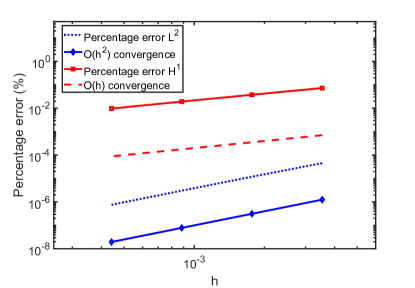
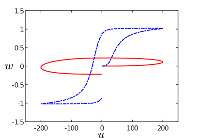
Figure 8: Left. Percentage errors in norms and versus the mesh-size $h$ for a fixed time-step $\Delta t/128$ (log-log scale). Right. Curve $w-u$ on a boundary point for $k=10^{3}$ (dashed line) and $k=0$ (solid line).

5.2 Numerical solution for different k-values

In this section we illustrate the behavior of the numerical solution to problem (47) for different configurations of the dynamic Preisach model. As we notice in Section 3, the evolution of the dynamic relay and, accordingly, the dynamic Preisach model, varies with respect to the velocity of the input and the relay slope $k$ (cf. Figures 2, 3 and 7). We have computed the solution of problem (47) where we have only changed the slope $k$ of the dynamic Preisach model. For the considered examples $k=1$ and $k=10^{3}$. Figures 9 and 10 show fields $u$ and $w$ solution to problem (47). From Figure 10 (bottom) it can be seen that changes in $w$ are smaller when $k=1$. This behavior is expected as the size of the $u-w$ cycle decreases when the slope, k, decreases (see Figure 2). This is not the case for the $w$ field for $k=10^{3}$: it reaches values close to saturation (see Figures 10 (top) and 8 (left)).

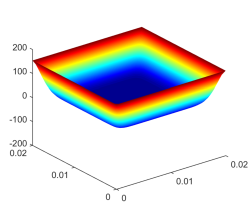
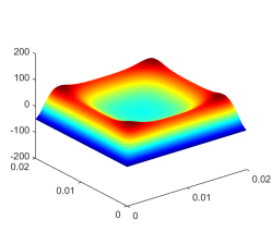
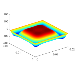
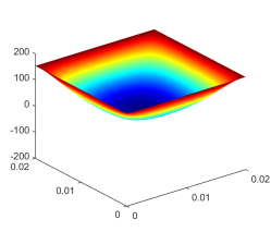
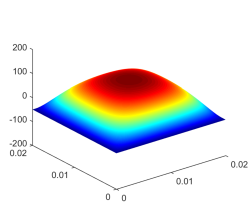
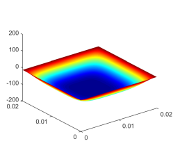
$t=0.002$s                           $t=0.0055$s                           $t=0.01$s

Figure 9: $u$-field solution to problem (47) for $k=10^{3}$ (top) and $k=1$ (bottom).

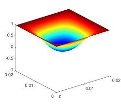
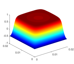
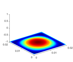
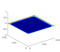
$t=0.002$s                           $t=0.0055$s                           $t=0.01$s

Figure 10: $w$-field solution to problem (47) for $k=10^{3}$ (top) and $k=1$ (bottom).

6 Conclusion

In this paper, we have introduced a functional analytic framework to study the dynamic Preisach model presented in [6]. This framework allow us to prove properties of the operator that can be used to study a wide range of hysteresis phenomena. In particular, and motivated by electromagnetic field equations, we study the well posedness of a family of PDE’s involving hysteresis. We have noticed that, even though the analysis is similar to the one applied for the classical Preisach model, key changes need to be done for the dynamic case. We also propose a numerical scheme to approximate a parabolic problem with dynamic Hysteresis. The numerical results presented in sections 3 and 5 help us to become familiar with the role of the $k$-value and the speed of the input in the dynamic Preisach model and how this parameter affects the solution of a PDE. A better understanding of the dynamic behavior of solution in processes with hysteresis is essential to understand the process itself and to develop appropriate numerical approximations.

Appendix A Proof of Theorem 2.1

Let us introduce the Lipschitz-continuous approximation of the multi-valued function $\partial\chi_{[-1,1]}$ defined by

$$(\partial\chi_{[-1,1]})_{\mu}(x)=\left\{\begin{array}[]{ll}\displaystyle\frac{x+1}{\mu}&\mbox{ if }x\leq-1,\\ \displaystyle 0&\mbox{ if }-1<x<1,\\ \displaystyle\frac{x-1}{\mu}&\mbox{ if }x\geq 1.\end{array}\right.$$

Actually, $(\partial\chi_{[-1,1]})_{\mu}$ is the so-called Yosida regularization of the multi-valued operator $\partial\chi_{[-1,1]}$. We notice that

$$(\partial\chi_{[-1,1]})_{\mu}(x)=\frac{x-P_{[-1,1]}(x)}{\mu}\quad\forall x\in\mathbb{R}$$ (48)

where $P_{[-1,1]}$ denotes the projection on the interval $[-1,1]$.

Let us consider an approximation of the Cauchy problem (20) defined as

$$\dfrac{dy_{\mu}}{dt}(t)+(\partial\chi_{[-1,1]})_{\mu}(y_{\mu}(t))=g_{\rho}(u(t)),$$ (49)

$$y(0)=\xi.$$ (50)

Since $g_{\rho}\in\mathrm{L}^{2}(0,T)$ and $(\partial\chi_{[-1,1]})_{\mu}$ is Lipschitz-continuous this problem has a unique solution from the Picard-Lipschitz Theorem. Moreover $y_{\mu}\in\mathrm{H}^{1}(0,T)$. In order to pass to the limit as $\mu\rightarrow 0$ let us obtain some a priori estimates. For this purpose we multiply both sides by $y_{\mu}(t)$. We have

$$\dfrac{dy_{\mu}}{dt}(t)y_{\mu}(t)+(\partial\chi_{[-1,1]})_{\mu}(y_{\mu}(t))y_{\mu}(t)=g_{\rho}(u(t))y_{\mu}(t)$$

and then

$$\frac{1}{2}\frac{d}{dt}|y_{\mu}(t)|^{2}\leq|g_{\rho}(u(t))||y_{\mu}(t)|.$$

From Gronwall’s inequality we deduce

$$|y_{\mu}(t)|\leq C\quad\forall t\in(0,T)$$

for some constant $C$. Next, we multiply (49) by $\frac{dy_{\mu}}{dt}(t)$. We get

$$|\frac{dy_{\mu}}{dt}(t)|^{2}+(\partial\chi_{[-1,1]})_{\mu}(y_{\mu}(t))\frac{dy_{\mu}}{dt}(t)=g_{\rho}(u(t))\frac{dy_{\mu}}{dt}(t).$$ (51)

From the chain rule we have

$$(\partial\chi_{[-1,1]})_{\mu}(y_{\mu}(t))\frac{dy_{\mu}}{dt}(t)=\frac{d}{dt}(\chi_{[-1,1]})_{\mu}(y_{\mu}(t)),$$

where $(\chi_{[-1,1]})_{\mu}(x)$ is a primitive of $(\partial\chi_{[-1,1]})_{\mu}(x)$. More precisely,

$$(\chi_{[-1,1]})_{\mu}(x)=\left\{\begin{array}[]{ll}\displaystyle\frac{(x+1)^{2}}{2\mu}&\mbox{ if }x\leq-1,\\ \displaystyle 0&\mbox{ if }-1<x<1,\\ \displaystyle\frac{(x-1)^{2}}{2\mu}&\mbox{ if }x\geq 1.\end{array}\right.$$

Since $(\chi_{[-1,1]})_{\mu}$ is non-negative, (51) yields

$$\int_{0}^{T}|\frac{dy_{\mu}}{dt}(t)|^{2}\,dt\leq\Big{(}\int_{0}^{T}|g_{\rho}(u(t))|^{2}dt\Big{)}^{1/2}\Big{(}\int_{0}^{T}|\frac{dy_{\mu}}{dt}|^{2}(t)\,dt\Big{)}^{1/2}$$

and hence

$$\|\frac{dy_{\mu}}{dt}\|_{\mathrm{L}^{2}(0,T)}\leq\|g_{\rho}\|_{\mathrm{L}^{2}(0,T)}.$$

Thus, the set $\{y_{\mu}\}$ is bounded in $\mathrm{H}^{1}(0,T)$ which implies that there exists $y\in\mathrm{H}^{1}(0,T)$ and a subsequence $\{y_{\mu_{n}}\}$ such that

$$\{y_{\mu_{n}}\}\mbox{ converges to }y\mbox{ weakly in }\mathrm{H}^{1}(0,T)\mbox{ and strongly in }\mathrm{L}^{2}(0,T).$$

Let

$$q_{\mu}:=(\partial\chi_{[-1,1]})_{\mu}(y_{\mu}(t)).$$

This means

$$q_{\mu}(t)\Big{(}x-y_{\mu}(t)\Big{)}\leq\Big{(}\chi_{[-1,1]}\Big{)}_{\mu}(x)-\Big{(}\chi_{[-1,1]}\Big{)}_{\mu}(y_{\mu}(t))\quad\forall x\in\mathbb{R}.$$ (52)

Besides, since $\displaystyle q_{\mu}=g_{\rho}(u(t))-\dfrac{dy_{\mu}}{dt}(t)$ then the set $\{q_{\mu}\}$ is bounded in $\mathrm{L}^{2}(0,T)$ and hence there exists $q\in\mathrm{L}^{2}(0,T)$ and a subsequence $\{q_{\mu_{n}}\}$ such that

$$\{q_{\mu_{n}}\}\mbox{ converges to }q\mbox{ weakly in }\mathrm{L}^{2}(0,T).$$

Passing to the limit in (49) we get

$$\dfrac{dy}{dt}(t)+q(t)=g_{\rho}(u(t)).$$ (53)

Now the goal is to prove that $q(t)\in\partial\chi_{[-1,1]}(y(t))$ a.e. in $[0,T]$. For this purpose we notice that, since $\{q_{\mu}\}$ is bounded in $\mathrm{L}^{2}(0,T)$, then (48) yields

$$\lim_{n\rightarrow\infty}\{P_{[-1,1]}(y_{\mu_{n}})\}=y\mbox{ strongly in }\mathrm{L}^{2}(0,T),$$

which in particular implies $-1\leq y(t)\leq 1\ \forall t\in[0,T]$. Now, let pass to the limit in (52) for $\mu=\mu_{n}$. Firstly, we have

$$0\leq\int_{0}^{T}\Big{(}\chi_{[-1,1]}\Big{)}_{\mu_{n}}(y_{\mu_{n}}(t))\,dt\leq-\int_{0}^{T}q_{\mu_{n}}(t)\big{(}z(t)-y_{\mu_{n}}(t)\big{)}\,dt+\int_{0}^{T}\Big{(}\chi_{[-1,1]}\Big{)}_{\mu_{n}}(z(t))\,dt,$$ (54)

for all $z\in\mathrm{L}^{2}(0,T)$. Then,

$$0\leq-\int_{0}^{T}q(t)\big{(}z(t)-y(t)\big{)}\,dt+\int_{0}^{T}\chi_{[-1,1]}(z(t))\,dt$$ (55)

because of the strong convergence of $\{y_{\mu_{n}}\}$, the weak convergence of $\{q_{\mu_{n}}\}$ and the fact that

$$\lim_{n\rightarrow\infty}\int_{0}^{T}\Big{(}\chi_{[-1,1]}\Big{)}_{\mu_{n}}(z(t))\,dt=\int_{0}^{T}\chi_{[-1,1]}(z(t))\,dt.$$

Finally, since $|y(t)|\leq 1$, then $\chi_{[-1,1]}(y(t))=0\,\forall t$ and we deduce from (55)

$$\int_{0}^{T}q(t)\big{(}z(t)-y(t)\big{)}\,dt\leq\int_{0}^{T}\chi_{[-1,1]}(z(t))\,dt-\int_{0}^{T}\chi_{[-1,1]}(y(t))\,dt$$

and then $q(t)\in\partial\chi_{[-1,1]}(y(t))\,\mbox{ a.e. in }(0,T)$.

Let us prove uniqueness. Assume that $y_{1}(t)$ and $y_{2}(t)$ are two solutions of (49), (50). Firstly $y_{1}(0)-y_{2}(0)=0$ and there exist $q_{i}(t)\in\partial\chi_{[-1,1]}(y_{i}(t)),\ i=1,2$ such that

$$\dfrac{dy_{i}}{dt}(t)+q_{i}(t)=g_{\rho}(u(t)),\ i=1,2.$$

Let us subtract the above equations for $i=1,2$ and then make the scalar product by $y_{1}-y_{2}$. We get

$$\frac{1}{2}\int_{0}^{t}\frac{d}{ds}|y_{1}(s)-y_{2}(s)|^{2}\leq 0$$

because,

$$\int_{0}^{t}(q_{1}(s)-q_{2}(s))(y_{1}(s)-y_{2}(s))\,dt\geq 0,$$

as $\partial\chi_{[-1,1]}$ is monotone. Hence,

$$|y_{1}(t)-y_{2}(t)|^{2}\leq|y_{1}(0)-y_{2}(0))|^{2}=0,$$

which finishes the proof.

References

- [1] F. Baronti, N. Femia, R. Saletti, C. Visone, and W. Zamboni. Hysteresis modeling in li-ion batteries. IEEE Trans. Magn., 50(11):1–4, 2014.
- [2] V. Basso, G. Bertotti, O. Bottauscio, F. Fiorillo, M. Pasquale, M. Chiampi, and M. Repetto. Power losses in magnetic laminations with hysteresis: Finite element modeling and experimental validation. J. Appl. Phys., 81(8):5606–5608, 1997.
- [3] A. Bermúdez, L. Dupré, D. Gómez, and P. Venegas. Electromagnetic computations with preisach hysteresis model. Finite Elem. Anal. Des., 126:65–74, 2017.
- [4] A. Bermúdez, D. Gómez, R. Rodríguez, and P. Venegas. Mathematical analysis and numerical solution of axisymmetric eddy-current problems with preisach hysteresis model. Rend. Semin. Mat. Univ. Politec. Torino, 72(1-2):73–117, 2014.
- [5] A. Bermúdez and C. Moreno. Duality methods for solving variational inequalities. Comput. Math. Appl., 7:43–58, 1981.
- [6] G. Bertotti. Dynamic generalization of the scalar preisach model of hysteresis. IEEE Trans. Magn., 28(5):2599–2601, 1992.
- [7] G. Bertotti. Hysteresis in Magnetism. Academic Press, 1998.
- [8] G. Bertotti and M. Pasquale. Physical interpretation of induction and frequency dependence of power losses in soft magnetic materials. IEEE Trans. Magn., 28(5):2787–2789, 1992.
- [9] O. Bottauscio, M. Chiampi, D. Chiarabaglio, and M. Repetto. Preisach-type hysteresis models in magnetic field computation. Physica B, 275(1-3):34–39, 2000.
- [10] H. Brézis. Opérateurs maximaux monotones et semi-groupes de contractions dans les espaces de Hilbert. North-Holland, 1973.
- [11] M. Brokate and J. Sprekels. Hysteresis and Phase Transitions. Springer, Berlin, 1996.
- [12] E. Della Torre. Magnetic Hysteresis. IEEE Press, New York, 1999.
- [13] L. Dupré, G. Bertotti, V. Basso, F. Fiorillo, and J.A.A Melkebeek. Generalisation of the dynamic preisach model toward grain oriented FeSi alloys. Physica B: Condensed Matter, 275(1):202 – 206, 2000.
- [14] L. Dupré, G. Bertotti, and J.A.A. Melkebeek. Dynamic preisach model and energy dissipation in soft magnetic materials. IEEE Trans. Magn., 34(4, 1):1168–1170, 1998.
- [15] M. Eleuteri. Well-posedness results for a class of partial differential equations with hysteresis arising in electromagnetism. Nonlinear Anal-Real, 8(5):1494 – 1511, 2007.
- [16] M. Eleuteri and J. Kopfová. Uniqueness and decay estimates for a class of parabolic partial differential equations with hysteresis and convection. Nonlinear Anal., 73(1):48–65, 2010.
- [17] J. A. Ewing. X. experimental researches in magnetism. Philos. Trans. R. Soc. Lond., 176:523–640, 1885.
- [18] P. Gurevich and W. Jäger. Parabolic problems with the Preisach hysteresis operator in boundary conditions. J. Differential Equations, 247(11):2966–3010, 2009.
- [19] J. K. Hale. Ordinary differential equations. Robert E. Krieger Publishing Co., Inc., Huntington, N.Y., second edition, 1980.
- [20] V. Hassani, T. Tjahjowidodo, and N. D. Thanh. A survey on hysteresis modeling, identification and control. Mech. Syst. Signal Proc., 49(1-2, SI):209–233, 2014.
- [21] M. Hintermüller, K. Ito, and K. Kunisch. The primal-dual active set strategy as a semismooth Newton method. SIAM J. Optim., 13(3):865–888 (2003), 2002.
- [22] P. Kordulová. Water flow through unsaturated porous media with hysteresis. Nonlinear Anal-Real, 12(6):3125 – 3134, 2011.
- [23] M.A. Krasnosel’skiĭ and A.V. Pokrovskiĭ. Systems with Hysteresis. Springer, Berlin, 1989. (Russian edition, Nauka, Moscow (1983)).
- [24] P. Krejčí. Evolution variational inequalities and multidimensional hysteresis operators. In Nonlinear differential equations, volume 404 of Res. Notes Math., pages 47–110. Chapman & Hall/CRC, London, 1999.
- [25] P. Krejčí, J. P. O’Kane, A. Pokrovskii, and D. Rachinskii. Properties of solutions to a class of differential models incorporating Preisach hysteresis operator. Phys. D, 241(22):2010–2028, 2012.
- [26] M. Kuczmann. Dynamic Preisach model identification applying FEM and measured BH curve. COMPEL, 33(6):2043–2052, 2014.
- [27] J.L. Lions. Quelques méthodes de résolution des problèmes aux limites non linéaires. Dunod, Gauthier-Villars, Paris, 1969.
- [28] V. A. Lubarda, D. Šumarac, and D. Krajcinovic. Preisach model and hysteretic behaviour of ductile materials. European J. Mech. A Solids, 12(4):445–470, 1993.
- [29] J. W. Macki, P. Nistri, and P. Zecca. Mathematical Models for Hysteresis. SIAM Review, 35(1):94–123, 1993.
- [30] G. Marinoschi. The diffusive form of Richards’ equation with hysteresis. Nonlinear Anal-Real, 9(2):518 – 535, 2008.
- [31] I. D. Mayergoyz. Dynamic Preisach Model of hysteresis. IEEE Trans. Magn., 24(6):2925–2927, 1988.
- [32] I. D. Mayergoyz. Mathematical models of hysteresis. Springer-Verlag, New York, 1991.
- [33] A. Mielke and R. Rossi. Existence and uniqueness results for a class of rate-independent hysteresis problems. Math. Models Meth. Appl. Sci., 17(01):81–123, 2007.
- [34] D. A. Philips, L. Dupré, J. Cnops, and J. A. A. Melkebeek. The application of the preisach model in magnetodynamics: theoretical and practical aspects. J. Magn. Magn. Mater., 133(1):540 – 543, 1994.
- [35] F. Preisach. Über die magnetische nachwirkung. Zeitschrift für Physik,, 94:277–302, 1935.
- [36] A. Rao and A.R. Srinivasa. A two species thermodynamic Preisach model for the torsional response of shape memory alloy wires and springs under superelastic conditions. Int. J. Solids Struct., 50(6):887 – 898, 2013.
- [37] T. Roubíček. Non Linear Partial Differential Equations with Applications. Birkhäuser, 2005.
- [38] B. Schweizer. Hysteresis in porous media: Modelling and analysis. Interface Free Bound., 19(3):417–447, 2017.
- [39] R. E. Showalter, T. D. Little, and U. Hornung. Parabolic PDE with Hysteresis. Control Cybern., 25:631–643, 1996.
- [40] R. Van Keer, L. Dupré, and J. A. A. Melkebeek. On a numerical method for 2D magnetic field computations in a lamination with enforced total flux. J. Comput. Appl. Math., 72:179–191, 1996.
- [41] A. Visintin. Differential models of hysteresis, volume 111 of Applied Mathematical Sciences. Springer-Verlag, Berlin, 1994.
- [42] A. Visintin. Chapter 1 - Mathematical Models of Hysteresis. In Giorgio Bertotti and I. D. Mayergoyz, editors, The Science of Hysteresis, pages 1 – 123. Academic Press, Oxford, 2006.
- [43] Y. Yu, Z. Xiao, N. G. Naganathan, and R. V. Dukkipati. Dynamic preisach modelling of hysteresis for the piezoceramic actuator system. Mech. Mach. Theory, 37(1):75–89, 2002.