Scattering amplitudes versus potentials in nuclear effective field theory:
is there a potential compromise?

Abstract

In effective field theory physical quantities, in particular observables, are expressed as a power series in terms of a small expansion parameter. For non-perturbative systems, for instance nuclear physics, this requires the non-perturbative treatment of at least a part of the interaction (or the potential, if we are dealing with a non-relativistic system). This is not entirely trivial and as a consequence different interpretations on how to treat these systems have appeared. A practical approach is to expand the effective potential, where this potential is later fully iterated in the Schrödinger equation for obtaining amplitudes and observables. The expectation is that this will lead to observables that will have an implicit power counting expansion. Here we explicitly check whether the amplitudes are actually following the same power counting as the potential. It happens that reality does not necessarily conform to expectations and the amplitudes will often violate the power counting with which the potential has been expanded. A more formal approach is to formulate the expansion directly in terms of amplitudes and observables, which is the original aim of the effective field theory idea. Yet this second approach is technically complicated. We explore here the possibility of constructing potentials that when fully iterated will make sure that amplitudes indeed are expansible in terms of a small expansion parameter.

The derivation of nuclear forces from first principles is the central problem of nuclear physics. It is also a hard nut to crack and despite many breakthroughs it has not been solved yet, see Ref. Machleidt (2017) for a historical perspective. Nowadays the expression from first principles refers to a derivation of the nuclear force grounded on quantum chromodynamics (QCD), the fundamental theory of strong interactions. But QCD is not analytically solvable at the natural energy scales of hadronic and nuclear physics. There are strategies to deal with this problem, of which the two most prominent ones are lattice QCD Beane et al. (2011) and effective field theory (EFT) Bedaque and van Kolck (2002); Epelbaum et al. (2009); Machleidt and Entem (2011). Lattice QCD directly solves QCD numerically in a space-time lattice. EFT in contrast handles QCD in an indirect way by exploiting the symmetries and degrees of freedom of QCD at low energies. The most fertile idea within the EFT formalism for strong forces is that of chiral symmetry Bernard et al. (1995), which plays a crucial role in the description of low energy hadronic processes.

EFTs heavily rely on the idea of separation of scales: specific physical phenomena take place at a natural low energy scale $Q$, which can be distinguished from the high energy scale $M$ at which a more fundamental description will eventually take place. For nuclear and hadronic physics this low energy scale is the pion mass or the typical momenta of nuclei within a nucleus ($Q\sim 100-200\,{\rm MeV}$), while the high energy scale is the typical mass of most hadrons ($M\sim 0.5-1.0\,{\rm GeV}$) which is a consequence of QCD. The key feature of EFTs is that every physical quantity can be expressed as an expansion in powers of $Q/M$. The advantages of the EFT expansion cannot be understated: in principle we have control on the theoretical accuracy of a calculation. In practice the realization of this idea will inevitably run into technical complications, particularly in the case of nuclear physics. The subject of the present manuscript is how to deal with a few of these complications.

The fact that physical quantities are expansions is incredibly convenient for precision era nuclear physics (a term referring to recent advances in ab-initio methods Soma et al. (2013); Lähde et al. (2014); Hagen et al. (2014); Carlson et al. (2015); Binder et al. (2016); Hebeler et al. (2015); Hergert et al. (2016)), as this property enables us to understand the errors of the calculations Navarro Pérez et al. (2015); Furnstahl et al. (2015); Grießhammer (2016). Hence the growing interest in developing EFT-based descriptions of the nuclear force Epelbaum et al. (2015); Entem et al. (2017); Reinert et al. (2018). This expectation is however at odds with the current implementation of nuclear EFT, which is a consequence of the history of the field. A few decades ago the theoretical understanding of EFTs was perturbative (see Ref. Polchinski (1984) for a lucid exposition), as exemplified by chiral perturbation theory (ChPT), the EFT for low energy hadronic processes. However nuclear physics is non-perturbative, a point that is obvious from the existence of nuclei. The most popular implementation of nuclear EFT, the Weinberg counting Weinberg (1990, 1991), can be understood in hindsight as an inspired workaround of the theoretical problem of formulating an EFT for a non-perturbative physical system. Weinberg noticed that while amplitudes in nuclear physics are non-perturbative and it is not obvious how to expand them in EFT, in contrast the nuclear potential is perturbative and amenable to an EFT expansion. Thus a very sensible solution is to simply expand the nuclear potential in EFT and then use it in the Schrödinger equation as has always been done in nuclear physics.

The problem with this potential-based formulation is that strictly speaking is not a genuine EFT: the natural expectation is that a small correction in the potential will translate into a small correction in the amplitudes, but this has not been tested except in a few instances usually involving toy models Epelbaum and Gegelia (2009). Besides power counting, there is a second pillar for EFTs: renormalization group invariance (or cut-off independence). It can be argued indeed that power counting is merely a consequence of renormalization group invariance Birse et al. (1999); Birse (2006); Valderrama (2016). Yet a series of works have shown that it is probably not possible to meet the requirements of renormalization with the purely non-perturbative treatment of the potential Pavon Valderrama and Arriola (2006); Pavon Valderrama and Ruiz Arriola (2006). As already conjectured in Ref. Nogga et al. (2005), we now know that the mixture of non-perturbative and perturbative methods guarantees observables that have a good expansion and are RG invariant at the same time Long and van Kolck (2008); Valderrama (2011); Pavon Valderrama (2011); Long and Yang (2011, 2012a, 2012a, 2012b); Wu and Long (2018). That is, they lead to exactly what we expect of nuclear EFT.

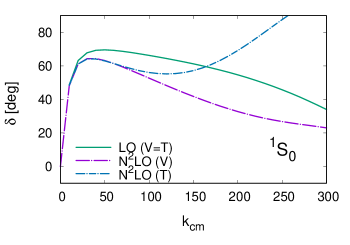
Figure 1: Phase shifts in the Weinberg counting, depending on whether we apply the power counting to the potential (V) or to the scattering amplitude (T). The calculation is done at ${\rm N^{2}LO}$ (i.e. including terms up to $\nu=3$ or $Q^{3}$) with a momentum space cutoff $\Lambda=400\,{\rm MeV}$ (see Appendix  A). At ${\rm LO}$ the potential- and amplitude-based expansions coincide, which in the figure is indicated with the notation $V=T$.

We mention in passing that a few authors have conjectured that the application of non-perturbative methods with a finite cut-off of an ideal size will lead to a well-defined expansion Epelbaum and Meissner (2013); Epelbaum and Gegelia (2009); Epelbaum et al. (2018). Yet this has only been illustrated with toy models Epelbaum and Gegelia (2009). The personal opinion of the author of the present manuscript is that these ideas are interesting but insufficient and that we should strive for full consistency though Valderrama (2019).

EFT expansion:

The purpose of the present manuscript is to check whether the potential-based approach to nuclear EFT complies with power counting expectations. That is, in the Weinberg prescription do small corrections to the EFT potential translate into small corrections to the amplitudes? In the Weinberg counting Weinberg (1990, 1991) the two-nucleon potential is expanded in terms of power counting as

$$V=\sum_{\nu=0}^{\nu_{\rm max}}V^{(\nu)}+\mathcal{O}\left({(\frac{Q}{M})}^{\nu_{\rm max}+1})\right)\,,$$ (1)

where the specific power counting used is naive dimensional analysis (NDA) and the error refers to the relative uncertainty. Depending on how many terms of the expansion we keep, we will say that we are working in leading order (${\rm LO}$), next-to-leading order ($\rm NLO$), next-to-next-to-leading order (${\rm N^{2}LO}$):

$$V^{\rm LO} = V^{(0)}\,,$$ (2)

$$V^{\rm NLO} = V^{(0)}+V^{(2)}\,,$$ (3)

$$V^{\rm N^{2}LO} = V^{(0)}+V^{(2)}+V^{(3)}\,,$$ (4)

plus analogous expressions for higher orders (notice that at $\nu=1$ there is no contribution to the EFT potential). In the Weinberg prescription the scattering amplitude is directly computed from the EFT potential:

$$T_{\rm W}=V+V\,G_{0}\,T\,,$$ (5)

where depending on where we cut the expansion we will talk about $T_{\rm W}^{\rm LO}$, $T_{\rm W}^{\rm NLO}$, $T_{\rm W}^{\rm N^{2}LO}$ and so on. There are a few technicalities involved in the previous process. One is that the EFT potential is singular and has to be regularized for its proper use within the Lippmann-Schwinger equation. Another is that the EFT potential contains free parameters that have to be fitted to data. We will not cover the specific details at the moment as these are standard technical procedures (a brief overview is given in Appendix A).

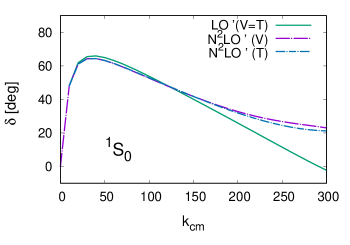
Figure 2: Phase shifts in an alternative power counting (read below), depending on whether we apply the power counting to the potential (V) or to the scattering amplitude (T). In this alternative power counting we have promoted the leading and subleading two-pion exchange diagrams to ${\rm LO}$ and demoted one-pion exchange to ${\rm N^{2}LO}$. We use the terms ${\rm LO}^{\prime}$ and ${\rm N^{2}LO^{\prime}}$ for referring to the orders in this counting. This alternative power counting is indistinguishable from the Weinberg one when expanding in terms of the potential.

If power counting is really working for the potential, the natural expectation is that the subleading contributions will be smaller than the leading order ones for the momenta at which the expansion is expected to work. That is, the scattering amplitude can be expanded in terms of the power counting

$$T_{\rm EFT}=\sum_{\nu=0}^{\nu_{\rm max}}T^{(\nu)}+\mathcal{O}\left({(\frac{Q}{M})}^{\nu_{\rm max}+1})\right)\,,$$ (6)

in analogy to what happens with the potential. This in turns means that the scattering amplitude should be perturbatively expansible, where each term in the expansion can be computed as

$$T^{(0)} = V^{(0)}+V^{(0)}\,G_{0}\,T^{(0)}\,,$$ (7)

$$T^{(2)} = \left(1+T^{(0)}\,G_{0}\right)\,V^{(2)}\left(\,G_{0}\,T^{(0)}+1\right),$$ (8)

$$T^{(3)} = \left(1+T^{(0)}\,G_{0}\right)\,V^{(3)}\left(\,G_{0}\,T^{(0)}+1\right),$$ (9)

plus more involved expression at higher orders (notice that the expressions above are relatively simple because the $\nu=1$ contribution to the EFT potential cancels, which means that up to $\nu=3$ first order perturbation theory is enough).

This means in particular that the a priori assumptions about power counting can indeed be tested a posteriori. For this we simply have to compare the T-matrix obtained with the standard Weinberg prescription with the T-matrix obtained from the perturbative expansion and check that their difference is higher order

$$|T_{W}-T_{\rm EFT}|\sim\mathcal{O}\left({(\frac{Q}{M})}^{\nu_{\rm max}+1})\right)\,.$$ (10)

For this we only have to adapt the existing frameworks for perturbative calculations Valderrama (2011); Pavon Valderrama (2011); Long and Yang (2011, 2012a, 2012b) to this particular case. In practice, instead of the $T$-matrix, we will compute the phase shift for a particular partial wave, where for illustrative purposes I will consider the ${}^{1}S_{0}$ channel at ${\rm N^{2}LO}$. The Weinberg amplitude $T_{W}$ is constructed by fitting the contact-range couplings of the EFT potential to the ${}^{1}S_{0}$ phase shifts obtained from a partial wave analysis (PWA) or a phenomenological potential. In particular we use the Nijmegen II potential Stoks et al. (1994) — equivalent to the Nijmegen PWA Stoks et al. (1993) — for this purpose. The Nijmegen PWA Stoks et al. (1993) has been recently improved upon by the more recent PWA of the Granada group Navarro Pérez et al. (2013a) and its phase-equivalent nuclear potentials Navarro Pérez et al. (2013b, 2015), but the specific choice of what data to fit is unessential for out discussion. The ${\rm LO}$ EFT amplitude $T_{\rm EFT}$ is constructed as the Weinberg one at the same order, while for the subleading corrections we determine the contact-range couplings by fitting to the phase shifts obtained from the subleading Weinberg amplitude $T_{W}$. That is, at the end we are comparing theory with theory (in the spirit of another recent proposal for analyzing power counting Grießhammer (2016)).

The outcome of this analysis can be seen in Fig. 1, where a clear breakdown of the assumed power counting happens at relatively low momenta. The potential- and amplitude-based expansions use a Gaussian regulator in p-space with a cutoff $\Lambda=400\,{\rm MeV}$. It can be seen that when amplitudes are expanded according to power counting, the Weinberg power counting is only preserved up to center-of-mass momenta of $100{\rm MeV}$ give or take. The amplitude-based expansion has been fitted to the potential-based phase shifts in the center-of-mass momentum range $k_{cm}=20-60\,{\rm MeV}$, where extending the range to higher momenta does not improve the visual appearance of the fits in Fig. 1 (but definitely spoils the agreement at low momenta). For further details of the calculation, we refer to Appendix A. We do not show the Nijmegen II phase shifts as they are not important in this context: they are merely used as a proxy for the calculation of $T_{W}$, but the focus is the comparison between $T_{W}$ and $T_{\rm EFT}$. Regarding the $\rm NLO$ phase shifts, we do not show them either as they are qualitatively similar to the $\rm N^{2}LO$ ones. We do not consider $\rm N^{3}LO$ and higher orders in the Weinberg counting either because they require second order perturbation theory for the finite-range potential.

Power counting breakdown:

As a matter of fact we can use perturbation theory to further analyze the actual power counting behaviour of the amplitudes against the nominal one in the potential. For instance, we can play the following game: exchange the orders of one and two pion exchange in the EFT expansion. That is, we consider a hypothetical power counting in which the two pion exchange piece of the EFT potential is ${\rm LO}$, while the one pion exchange piece is demoted to subleading orders ($\rm N^{2}LO$ for instance). The power counting of the contact-range interactions is left unchanged though. If we consider only the ${\rm N^{2}LO}$ potential-based expansion, this hypothetical power counting is indistinguishable from the Weinberg counting. The outcome is this game is shown in Fig. 2, which reproduces relatively well the ${\rm N^{2}LO}$ Weinberg phase shifts. This is indeed shocking to say the least, because it implies that the actual power counting of the amplitudes is radically different than the power counting assumed for the potential. We will call this type of behaviour power counting breakdown or power counting extravaganza, to indicate the relative freedom of the actual power counting in the amplitudes. This scenario was first considered in Ref. Valderrama (2010).

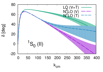
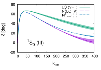
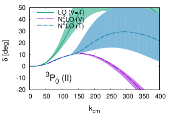
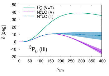
Figure 3: Phase shifts for second Epelbaum et al. (2004a, b) and third generation Gezerlis et al. (2014) $\rm N^{2}LO$ potentials in the Weinberg counting, depending on whether we expand the potential (V) or the scattering amplitude (T). For the second generation potential of Refs. Epelbaum et al. (2004a, b) the Lippmann-Schwinger and SFR cutoffs are $\Lambda=450-650$ and $\tilde{\Lambda}=500-700\,{\rm GeV}$, with the central phase shifts calculated for $(\Lambda,\tilde{\Lambda})=(550,600)\,{\rm MeV}$. The third generation potential of Ref. Gezerlis et al. (2014) is formulated in coordinate space and it uses a Gaussian type cutoff in the range $R_{c}=1.0-1.2\,{\rm fm}$ and the SFR cutoff $\tilde{\Lambda}=1.0-1.4\,{\rm GeV}$. In the figures for the potential of Ref. Gezerlis et al. (2014) we have generated the error bands from varying $R_{c}$ only, leaving the SFR cutoff unchanged at the value $\tilde{\Lambda}=1.0\,{\rm GeV}$. We compute the phase shifts for the ${}^{1}S_{0}$ and ${}^{3}P_{0}$ partial waves, where the roman numeral in parentheses indicates whether the calculation corresponds to the second (II) or third generation (III) potential.

Analyzing EFT potentials that follow the Weinberg counting:

The breakdown of power counting is not universal to all amplitudes in the Weinberg prescription. Whether this happens or not actually depends on the interplay between the regulator and the cut-off, and while in a few cases there will be severe power counting breakdowns, in other cases power counting will work perfectly fine. Besides, from the initial Weinberg potential of Ray, Ordoñez and van Kolck Ordonez et al. (1994, 1996) (which can be understood as a proof of concept of the applicability of EFT ideas to nuclear physics) till the present day, the EFT descriptions of the nuclear forces have improved dramatically. For discussion purposes we will refer to the work of Ray, Ordoñez and van Kolck Ordonez et al. (1994, 1996) as the first generation of EFT potentials, which contains more or less the same ingredients as the calculation of Fig. 1 (except for the use of time-ordered perturbation theory and the explicit inclusion of isobar $\Delta$ excitations in Ref. Ordonez et al. (1996)). For this reason, though we have not explicitly analyzed it, we do not expect the first generation potential of Ref. Ordonez et al. (1996) to do much better in terms of power counting than the calculation of Fig. 1. The first ${\rm N^{2}LO}$ potential that signaled the quantitative viability of Weinberg’s prescription fifteen years ago is the one from Epelbaum, Glöckle and Meißner Epelbaum et al. (2004a, b), which we will refer to as a second generation EFT potential and features an energy independent potential and an improved regularization and renormalization process owing to the inclusion of spectral function regularization (SFR). The more recent ${\rm N^{2}LO}$ potential of Gezerlis et al. Gezerlis et al. (2014) is local and pushes the SFR cutoff to harder values. We will refer to it as a third generation potential.

Here we analyze the power counting of the second and third generation potentials for the ${}^{1}S_{0}$ and ${}^{3}P_{0}$ partial waves at $\rm N^{2}LO$. The choice of the ${}^{1}S_{0}$ and ${}^{3}P_{0}$ channels is because these are two partial waves for which power counting is expected to deviate from Weinberg, at ${\rm LO}$ for the ${}^{3}P_{0}$ case Nogga et al. (2005) and at subleading orders for the ${}^{1}S_{0}$ case Valderrama (2011); Long and Yang (2012b). The result of this analysis is shown in Fig. 3, where we can check that power counting is still failing for the amplitudes but this failure is nonetheless less severe as the one in Fig. 1. Not only that, there is indeed a marked improvement of the implicit power counting features of the third generation potential over the second generation one, particularly in the ${}^{3}P_{0}$ partial wave.

The technical details of the previous comparison are similar to the ones behind the calculation of Fig. 1 and can be consulted in Appendices A and B for the second and third generation potentials, respectively. There are a few details that are worth commenting now. For the finite-range piece of the EFT potential, i.e. one- and two-pion exchange, we use the same conventions and regularizations as in the original potentials Epelbaum et al. (2004a, b); Gezerlis et al. (2014). In particular we include SFR for the two-pion exchange piece of the EFT potential. The perturbative amplitude $T_{\rm EFT}$ for the ${}^{1}S_{0}$ partial wave is fitted to the corresponding ${\rm N^{2}LO}$ amplitude in the range $k_{\rm cm}=40-120\,{\rm MeV}$, where $k_{cm}$ is the center of mass momentum. In the case of the ${}^{3}P_{0}$ partial wave, the range is $k_{\rm cm}=40-120\,{\rm MeV}$ for the second generation EFT potential and $k_{\rm cm}=50-150\,{\rm MeV}$ for the third generation one. It is possible to fit for larger momenta, but this does not translate into better phase shifts when expanding in terms of amplitudes (on the contrary, it only worsens the matching between $T_{W}$ and $T_{\rm EFT}$). There is also a difficulty in the EFT fit to the ${}^{3}P_{0}$ phase shift of Gezerlis et al. Gezerlis et al. (2014), which actually depends on which representation we use for the contact-range potential. The third generation potential of Ref. Gezerlis et al. (2014) is local, which implies a contact-range potential that has a central, spin-spin, tensor and spin-orbit component. Yet the projection into a particular partial wave does not discriminate among these operators. For this reason we have settled into a spin-orbit form of the contact-range interaction, which actually provides a better fit than a tensor form. A more detailed discussion is presented in Appendix B.5.

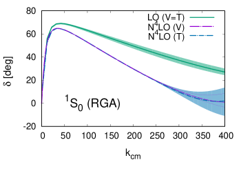
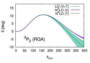
Figure 4: Phase shifts in the power counting of the pionful EFT of Refs. Valderrama (2011); Pavon Valderrama (2011); Long and Yang (2011, 2012a, 2012b), depending on whether we expand in the potential (V) or in the scattering amplitude (T). The calculation is done at $\rm N^{4}LO$ (i.e. including contributions up to $\nu=3$ or $Q^{3}$) and uses a Gaussian type regulator in coordinate space with $R_{c}=1.1-1.3\,{\rm fm}$, where the unregularized EFT potential is calculated in dimensional regularization (equivalent to taking $\tilde{\Lambda}\to\infty$ in SFR).

Operator	Weinberg	Pionful RGA/EFT(s)
$G_{0}$	$Q^{0}$	$Q^{1}$
$V_{\rm OPE}$	$Q^{0}$	$Q^{-1}$
$V_{\rm TPE(L)}$	$Q^{2}$	$Q^{2}$
$V_{\rm TPE(SL)}$	$Q^{3}$	$Q^{3}$
$C_{0}$	$Q^{0}$	$Q^{-1}$
$C_{2}(p^{2}+{p^{\prime}}^{2})$	$Q^{2}$	$Q^{0}$
$C_{4}(p^{2}+{p^{\prime}}^{2})$	$Q^{4}$	$Q^{2}$
$C_{1}\vec{p}\cdot{\vec{p}\,}^{\prime}$	$Q^{2}$	$Q^{-1}$
$C_{3}\vec{p}\cdot{\vec{p}\,}^{\prime}\,(p^{2}+{p^{\prime}}^{2})$	$Q^{4}$	$Q^{3/2}$

Table 1: Power counting of different contributions in the Weinberg counting and in the pionful EFT derived from Refs. Birse (2006); Valderrama (2011); Long and Yang (2012b). We only consider the ingredients relevant for the calculation of the ${}^{1}S_{0}$ and ${}^{3}P_{0}$ phase shifts, which are the propagator $G_{0}$, the one- and two-pion exchange potentials (leading and subleading), $V_{\rm OPE}$, $V_{\rm TPE(L)}$, $V_{\rm TPE(SL)}$ and the contact-range interactions in the ${}^{1}S_{0}$ and ${}^{3}P_{0}$ partial waves, denoted by $C_{0}$, $C_{2}$, $C_{4}$ and $C_{1}$, $C_{3}$ respectively. It must be said that Refs. Birse (2006); Valderrama (2011); Long and Yang (2012b) do not agree on the details and that the version presented here is closest to Refs. Valderrama (2011); Pavon Valderrama (2011), except for the counting of the $C_{2}$ coupling in the singlet for which we follow Ref. Valderrama (2016).

Building EFT potentials that preserve power counting:

Now we consider the power counting that stems from RG invariance Birse (2006); Valderrama (2011); Pavon Valderrama (2011); Long and Yang (2011, 2012a, 2012b) instead of NDA. It can be said that the application of this power counting to nucleon-nucleon scattering is still in the proof of concept phase Valderrama (2011); Pavon Valderrama (2011); Long and Yang (2011, 2012a, 2012b), a situation analogous to that of Weinberg’s counting twenty years ago. Though originally intended for expanding amplitudes, this power counting can be used to construct a potential in the same way as in the case of the Weinberg counting. Then the non-perturbative amplitudes obtained from this potential can also be reexpanded following the previous ideas, to check whether the power counting in the potential and the amplitudes coincide. There is however a certain degree of ambiguity in the power counting of pionful EFT, where different works display minor differences regarding the ordering of operators Birse (2006); Valderrama (2011); Pavon Valderrama (2011); Long and Yang (2011, 2012a, 2012b). Here I settle for the specific version of Ref. Valderrama (2016), which can be regarded as a maturation of the previous ideas of Refs. Valderrama (2011); Pavon Valderrama (2011). For concreteness the power counting conventions we employ for the ${}^{1}S_{0}$ and ${}^{3}P_{0}$ partial waves are written down in Table 1, where a comparison with the standard Weinberg counting is also provided. It is important to notice that in the pionful EFT of Table 1 the expansion begins at order $\nu=-1$, and that new couplings or new corrections to already existing couplings enter at each new order. For this reason the orders are labeled in a different way than in the Weinberg counting: $\nu=0$ is now ${\rm NLO}$, $\nu=1$ is ${\rm N^{2}LO}$, $\nu=2$ is ${\rm N^{3}LO}$ and $\nu=3$ is ${\rm N^{4}LO}$.

In this case we arrive at the results of Fig. 4, where we show the phase shifts for the potential-based and amplitudes-base EFT expansions at ${\rm N^{4}LO}$ in the power counting of the pionful EFT of Table 1. Notice that ${\rm N^{4}LO}$ in the pionful RGA corresponds to including the finite-range (pion) physics up to order $Q^{3}$, i.e. this type of calculation contains the same finite-range physics as the ${\rm N^{2}LO}$ calculations of Fig. 3. It can be appreciated that for the chosen cutoff window the potential- and amplitude-based approaches are compatible and lead to the same results. The potentials and amplitudes are regularized in coordinate space with the cutoff window is $R_{c}=1.1-1.3\,{\rm fm}$, where the explicit details are explained in Appendix A. The cutoff window of Fig. 4 is indeed a big larger than (but still pretty similar to) the one of the third generation potential of Ref. Gezerlis et al. (2014) (namely $R_{c}=1.0-1.2\,{\rm fm}$). In contrast with the idea of power counting extravaganza shown in Fig. 2, the situation in Fig. 4 could be labeled power counting preservation (or power counting bonanza). Notice that for generating Fig. 4 we have used the EFT potentials derived from dimensional regularization instead of the ones using SFR, where the explicit expressions have been taken form Ref. Rentmeester et al. (1999). We notice that this demonstrates the conjecture of Ref. Gezerlis et al. (2014) about the possibility of removing spectral function regularization in the future, albeit in a different power counting as the original one considered in Ref. Gezerlis et al. (2014). The choice of couplings for the finite-range piece of the chiral potential ($g_{A}$, $f_{\pi}$, $m_{\pi}$, $d_{18}$, $c_{1}$, $c_{3}$ and $c_{4}$) is identical to the one in Ref. Pavon Valderrama (2011). We also include the recoil corrections in the subleading piece of the two-pion exchange potential. In the amplitude-based approach the contact-range potential is iterated according to its power counting. This comment applies in particular to the $C_{2}\,(p^{2}+p^{\prime 2})$ operator, which is included in first order perturbation theory at ${\rm NLO}$, in second order at ${\rm N^{2}LO}$, and so on.

At this point it is also worth mentioning that there are EFT-inspired potentials which combine finite-range interactions up to order $Q^{3}$ with contact-range interactions up to order $Q^{4}$, for instance the recent potential of Ref. Piarulli et al. (2015). The inclusion of the higher order contact-range operators is reminiscent of the pionful power counting that is derived from RGA or perturbative renormalizability Birse (2006); Valderrama (2011); Long and Yang (2012b). Alternatively, a quick look at Table 1 illustrates the point. This potential might indeed be an accidental realization of the ideas promoted in this manuscript about finding a potential that preserves power counting when iterated. Yet for this to be true, it would be necessary to define what constitutes the ${\rm LO}$ of the potential of Ref. Piarulli et al. (2015) and to check whether their subleading pieces behave indeed as perturbations.

Conclusions:

We have analyzed whether the scattering amplitudes derived in the Weinberg prescription do actually follow the Weinberg power counting. The answer seems to be no, except for very low momenta (definitely below the expected range of applicability of this power counting), though particular potentials in the Weinberg prescription can do a better job for good regulator and cutoff choices. In particular the more recent potentials using the Weinberg prescription Gezerlis et al. (2014) fare noticeably better than the older ones Epelbaum et al. (2004a, b). The tool for this analysis are the distorted wave perturbative techniques that are normally used to construct scattering amplitudes following an explicit power counting Valderrama (2011); Pavon Valderrama (2011); Long and Yang (2011, 2012a, 2012b). Yet the present analysis is of an exploratory nature and a more definite conclusion will require a thorough analysis including more partial waves, considering second and higher order perturbation theory for the two-pion exchange potential and going beyond ${\rm N^{2}LO}$ (within the Weinberg counting).

There is a tension between traditional nuclear physics methods and nuclear EFTs with formal power counting. The former usually relies on purely non-perturbative methods, while the later requires that the subleading pieces of the interaction are treated in perturbation theory and renormalized accordingly. Here we have explicitly shown that it is possible to construct EFT-inspired potentials with good power counting properties. This provides a compromise between EFT and traditional approaches to nuclear physics. Of course a necessary condition is to follow the power counting derived from the RG analysis of pionful EFT Birse (2006); Valderrama (2011); Pavon Valderrama (2011); Long and Yang (2011, 2012a, 2012b); Valderrama (2016) (instead of NDA) when building this type of potential. The price to pay is that exact RG invariance is broken: the EFT-inspired potentials we are proposing here are only guaranteed to have good power counting properties for a particular cutoff range. But the advantages derived from RG invariance, in particular the possibility of a priori error estimations (crucial for precision nuclear physics), are preserved.

Appendix A Perturbation theory in p-space

First we explain perturbation theory as applied in p-space. The most prominent application is the EFT analysis of the phase shifts in the Weinberg counting, in particular the second generation $\rm N^{2}LO$ Weinberg potential of Refs. Epelbaum et al. (2004a, b). For this reason we will use here the power counting convention and notations of the Weinberg prescription. The starting point is the Lippmann-Schwinger equation

$$T=V+V\,G_{0}\,T\,,$$ (11)

which we expand according to the power counting of the potential and the T-matrix, see Eqs. (1) and (6). The resulting leading and subleading order Lippmann-Schwinger equations are the ones in Eqs. (7-9).

The relation of the full T-matrix with the phase shifts is given by

$$k\cot{\delta(k)}-ik=-\frac{2\pi}{\mu}\,\frac{1}{T(k)}\,,$$ (12)

which can change depending on how we normalize the T-matrix. We can simplify the previous relation to

$$\cot{\delta(k)}=-\frac{2\pi}{\mu k}\,{\rm Re}\left[\frac{1}{T(k)}\right]=-\frac{2\pi}{\mu k}\,\frac{1}{K(k)}\,.$$ (13)

where $K(k)$ is often called the K-matrix. Expanding according to the power counting we obtain at ${\rm LO}$ ($\nu=0$)

$$\cot{\delta^{(0)}(k)}=-\frac{2\pi}{\mu k}\,\frac{1}{K^{(0)}(k)}\,,$$ (14)

while at higher orders ($1\leq\nu<4$) we have

$$\frac{\delta^{(\nu)}(k)}{\sin^{2}{\delta^{(\nu)}}}=-\frac{2\pi}{\mu k}\,\frac{K^{(\nu)}(k)}{{K^{(0)}(k)}^{2}}\,,$$ (15)

where we have used again the K-matrix formalism.

In the ${}^{1}S_{0}$ partial wave the $\rm LO$ potential is the sum of the OPE potential and a momentum-independent contact term

$$\langle p|V^{(0)}({}^{1}S_{0})|p^{\prime}\rangle=C_{0}^{(-1)}+\langle p|V_{\rm OPE}^{{}^{1}S_{0}}|p^{\prime}\rangle\,,$$ (16)

while for the ${}^{3}P_{0}$ it only contains the OPE potential

$$\langle p|V^{(0)}({}^{3}P_{0})|p^{\prime}\rangle=\langle p|V_{\rm OPE}^{{}^{3}P_{0}}|p^{\prime}\rangle\,.$$ (17)

At $\rm NLO$ and ${\rm N^{2}LO}$ the contact-range piece of the potential in the ${}^{1}S_{0}$ and ${}^{3}P_{0}$ channels is given by

$$\langle p|V_{C}^{(\nu)}({}^{1}S_{0})|p^{\prime}\rangle = C_{0}^{(\nu)}+C_{2}^{(\nu)}\,(p^{2}+p^{\prime 2})\,,$$ (18)

$$\langle p|V_{C}^{(\nu)}({}^{3}P_{0})|p^{\prime}\rangle = C_{1}^{(\nu)}\,pp^{\prime}\,.$$ (19)

In turn the specific expressions for the $\rm NLO$ and ${\rm N^{2}LO}$ finite-range potential (with SFR) can be consulted in Refs. Epelbaum et al. (2004a, b). For solving the Lippmann-Schwinger equation or its perturbative expansion, the EFT potential is regularized as follows

$$\langle p|V(\Lambda)|p^{\prime}\rangle = \langle p|V_{\rm DR/SFR}|p^{\prime}\rangle\,f(\frac{p}{\Lambda})\,f(\frac{p^{\prime}}{\Lambda})\,,$$ (20)

where following Refs. Epelbaum et al. (2004a, b) we take $f(x)=e^{-x^{4}}$ and the original EFT potential, which might be the dimensional regularizarion (DR) or the SFR version, depending on the calculation.

Finally we mention that a very convenient feature of the perturbative corrections to the $T$-matrix is that they depend linearly on the contact-range couplings. In particular $T^{(\nu)}$ can be subdivided into a finite- and contact-range piece

$$T^{(\nu)}=T_{F}^{(\nu)}+T_{C}^{(\nu)}\,,$$ (21)

where $T_{C}^{(\nu)}$ can be written as

$$T_{C}^{(\nu)}({}^{1}S_{0}) = C_{0}^{(\nu)}T_{C_{0}}^{(\nu)}+C_{2}^{(\nu)}T_{C_{2}}^{(\nu)}\,,$$ (22)

$$T_{C}^{(\nu)}({}^{3}P_{0}) = C_{1}^{(\nu)}T_{C_{1}}^{(\nu)}\,,$$ (23)

for the ${}^{1}S_{0}$ and ${}^{3}P_{0}$ partial waves, respectively. This in turns simplifies the fitting procedure, see Appendix B.7 for further details.

Appendix B Perturbation theory in r-space

Here we explain how perturbation theory works in r-space. The principles are the same as in the p-space case, but the details are more complicated because we consider perturbation theory at higher orders. This is required for the description of the ${}^{1}S_{0}$ phase shifts in the power counting derived from the RGA of pionful EFT, see Table 1, which entails the iteration of the $C_{2}\,(p^{2}+p^{\prime 2})$ contact-range operator according to the counting, i.e. $\nu$-iterations (or $\nu$-loops) of $C_{2}\,(p^{2}+p^{\prime 2})$ at $N^{\nu+1}LO$. Though we are using perturbation theory in r-space for both the Weinberg counting and pionful RGA, the most representative application is the later. For this reason the notation will be adapted to the pionful RGA of Table 1.

B.1 Perturbative (Power Counting) Series

The starting point is the reduced Schrödinger equation for the $l$-wave

$$-u_{k}^{\prime\prime}(r)+\left[2\mu V_{\rm EFT}(r)+\frac{l(l+1)}{r^{2}}\right]\,u_{k}(r)=k^{2}u_{k}(r)\,,$$

where $u_{k}$ is the reduced wave function, $V_{\rm EFT}$ the EFT potential, $k$ the center-of-mass momentum, $l$ the orbital angular momentum and $\mu$ the reduced mass. The EFT potential and the wave function are expanded as a series

$$V_{\rm EFT}(r) = \sum_{\nu=-1}V^{(\nu)}(r)\,,$$ (25)

$$u_{k}(r) = \sum_{\nu=0}u^{(\nu)}_{k}(r)\,,$$ (26)

where the expansion of the reduced wave function begins at $\nu=0$. From this, we arrive at the following set of coupled differential equations

$$F^{(-1)}\,[u_{k}^{(0)}(r)] = 0\,,$$ (27)

$$F^{(-1)}\,[u_{k}^{(\nu)}(r)] = -2\mu\sum_{\begin{subarray}{c}\nu_{1},\nu_{2}\geq 0\\ \nu_{1}+\nu_{2}=\nu-1\end{subarray}}\,V^{(\nu_{1})}u_{k}^{(\nu_{2})}\,,$$ (28)

where the differential operator $F^{(-1)}$ is simply the ${\rm LO}$ reduced Schrödinger equation

$$F^{(-1)}\,[u_{k}] = -u_{k}^{{}^{\prime\prime}}+\left[2\mu V^{(-1)}+\frac{l(l+1)}{r^{2}}-k^{2}\right]\,u_{k}\,.$$

We are interested in the EFT series of the phase shifts

$$\delta(k)=\sum_{\nu=0}\delta^{(\nu)}(k)\,,$$ (30)

which we will calculate iteratively. We begin with $\nu=-1$ in the potential (i.e. $\nu=0$ in the wave function and phase shifts), for which the wave function behaves as

$$u_{k}^{(0)}\to\cot{\delta^{(0)}}\,\hat{j}_{l}(kr)-\hat{y}_{l}(kr)\,,$$ (31)

from which we extract the phase shift $\delta^{(0)}$, where $\hat{j}_{l}(x)=xj_{l}(x)$, $\hat{y}_{l}(x)=xy_{l}(x)$ with $j_{l}(x)$ and $y_{l}(x)$ the spherical Bessel functions. From this, we obtain $\delta^{(1)}$ as

$$[\cot{\delta}]^{(1)}=\frac{2\mu}{k}\,I_{k}^{(0)}$$ (32)

where $[\cot{\delta}]^{(1)}$ refers to the first term of the expansion

$$\cot{\delta}=\cot{(\sum_{\nu=0}\delta^{(\nu)})}=\sum_{\nu=0}\,[\cot{\delta}]^{(\nu)}\,,$$ (33)

which is the result of expanding the phase shift $\delta$ within the cotangent, and which leads to

$$[\cot{\delta}]^{(1)}=-(1+{\cot{\delta^{0}}}^{2})\,\delta^{(1)}\,.$$ (34)

$I_{k}^{(0)}$ the perturbative integral, which is given by

$$I^{(0)} = \int_{0}^{\infty}dr\,V^{(0)}\,{u_{k}^{(0)}}^{2}\,.$$ (35)

From this we can obtain the asymptotic form ($r\to\infty$) of the subleading correction to the reduced wave function at the following order in the EFT expansion

$$u^{(1)}_{k}(r)\to[\cot{\delta}]^{(1)}\,\hat{j}_{l}(kr)\,,$$ (36)

where, by integrating downwards towards $r=0$, we can compute the full subleading reduced wave function. If we assume that we have $\delta^{(0)}$, $\delta^{(1)}$, $\dots$, $\delta^{(\nu)}$ and $u_{k}^{(0)}$, $u_{k}^{(1)}$, $\dots$, $u_{k}^{(\nu)}$, we can obtain the $(\nu+1)$-th correction to the phase shift as

$$[\cot{\delta}]^{(\nu+1)}=\frac{2\mu}{k}\,I_{k}^{(\nu)}$$ (37)

where $[\cot{\delta}]^{(\nu+1)}$ is the $(\nu+1)$-th term in the expansion of Eq. (33). The perturbative integral is defined as

$$I^{(\nu)} = \int_{0}^{\infty}dr\,\left[V^{(\nu)}\,{u_{k}^{(0)}}^{2}+V^{(\nu-1)}u_{k}^{(0)}u_{k}^{(1)}+\dots\right]$$ (38)

$$= \int_{0}^{\infty}dr\,u_{k}^{(0)}\sum_{\begin{subarray}{c}\nu_{1},\nu_{2}\geq 0\\ \nu_{1}+\nu_{2}=\nu\end{subarray}}V^{(\nu_{1})}\,u_{k}^{(\nu_{2})}\,,$$

from which we obtain the asymptotic form of the $u_{k}^{(\nu+1)}$ reduced wave function as

$$u^{(\nu+1)}_{k}\to[\cot{\delta}]^{(\nu+1)}\,\hat{j}_{l}(kr)\,,$$ (39)

and then continue to the next order.

B.2 Are perturbative phase shifts uniquely defined?

A common misconception is that the perturbative phase shifts are not well-defined and rely on some sort of unitarization. In fact at first sight it looks like the definition of the perturbative phase shifts depends on the asymptotic normalization of the wave function. But this is merely apparent. If instead of the asymptotic normalization

$$u_{k}\to\cot{\delta}\,\hat{j}_{l}(kr)-\hat{y}_{l}(kr)\,,$$ (40)

we have used other normalization, for example

$$u_{k}\to\hat{j}_{l}(kr)-\tan{\delta}\,\hat{y}_{l}(kr)\,,$$ (41)

the final calculation of $\delta^{(\nu)}$ would have been the same (though it requires a bit of patience to check this explicitly at higher orders).

B.3 Regularization of the finite-range potential

The finite-range potential is regularized as in Ref. Gezerlis et al. (2014), that is, we multiply the EFT potential by

$$V_{\rm EFT}(r;R_{c})=(1-f(r;R_{c}))\,V_{\rm EFT}(r)\,,$$ (42)

with $f=e^{-(r/R_{c})^{2n}}$. For the power counting analysis of the potential of Ref. Gezerlis et al. (2014) we use $n=2$ and in addition the EFT potential is further regularized with SFR. For the power counting analysis of the pionful theory we use $n=3$ and the EFT potential that is obtained in dimensional regularization. We notice that the $n=2$ and $n=3$ exponents are not entirely arbitrary: the $Q^{2}$ and $Q^{3}$ EFT potentials diverge as $1/r^{5}$ and $1/r^{6}$ in dimensional regularization, or as $1/r^{3}$ in SFR. This means that $n=3$ and $n=2$ are the smallest exponents that lead to a regularized potential that is finite at the origin.

B.4 The S-wave contact-range potential

The standard (unregularized) representation of the contact-range potential for S-waves is a power series in terms of $p^{2}$ and ${p^{\prime}}^{2}$

$$\langle p^{\prime}|V_{C}|p\rangle = \sum_{n}C_{2n}P_{n}({p^{\prime}}^{2},{p}^{2})$$ (43)

$$= C_{0}+C_{2}(p^{2}+{p^{\prime}}^{2})$$

$$+ C_{4}(p^{4}+{p^{\prime}}^{4})+C_{4}^{\prime}p^{2}{p^{\prime}}^{2}+\dots$$

where $p^{\prime}$ and $p$ are the center-of-mass outgoing and incoming momenta of the nucleons and $P_{n}(x,y)$ is a polynomial of order ${n}$ of two variables such that $P_{n}(x,y)=P_{n}(y,x)$. At higher order there are terms that are equivalent in the pionless theory, for instance $C_{4}\,(p^{4}+p^{\prime 4})$ and $C_{4}^{\prime}\,p^{2}{p^{\prime}}^{2}$ as shown in Ref. Beane and Savage (2001). In the pionful theory they are suspected to be equivalent, but this has not been proven. Be it as it may, there is a certain arbitrariness in the representation of contact-range physics which can be used to devise more convenient representations.

Here we will use the local representation of proposed in Ref. Gezerlis et al. (2014), in which the S-wave contact-range potential is expressed as

$$V_{C}(\vec{q})=\sum_{n\geq 0}\,C_{2n}{\vec{q}\,}^{2n}\,.$$ (44)

When Fourier-transformed and regularized into r-space, the corresponding contact-range potential reads

$$V_{C}(r;R_{c})=\sum_{2n}\,C_{2n}^{(\nu)}{(-\Delta)}^{2n}\delta_{c}(r;R_{c})\,,$$ (45)

with $\Delta$ the Laplacian and

$$\delta_{c}({r};R_{c})=\frac{e^{-(r/R_{c})^{2n}}}{\frac{4}{3}\pi\,\Gamma(1+\frac{3}{2n})\,R_{c}^{3}}\,,$$ (46)

where owing to the central character of $\delta_{c}$, the Laplacian simplifies to

$$\Delta=\frac{d^{2}}{dr^{2}}+\frac{2}{r}\,\frac{d}{dr}\,.$$ (47)

For the EFT amplitudes corresponding to the local $\rm N^{2}LO$ Weinberg potential of Ref. Gezerlis et al. (2014) we use $n=2$, while for the pionful EFT calculation of Fig. 4 we use $n=3$.

B.5 The $P$-wave contact-range potential

The standard (unregularized) representation of the $l$-wave contact-range potential reads (after projection in the $l$-wave)

$$\langle p^{\prime},l|V_{C}|p,l\rangle = p^{l}{p^{\prime}}^{l}\sum_{n}C^{l}_{2n}P_{n}({p^{\prime}}^{2},{p}^{2})\,,$$ (48)

that is, exactly as the $S$-wave one except for the extra factors of $(pp^{\prime})^{l}$. By setting $l=1$ we particularize for the $P$-wave.

The previous representation is the most obvious one but it is also non-local. There are local representations though, as the one of Ref. Gezerlis et al. (2014), in which all the contact-range terms with two derivatives are written together as

$$V_{C}^{[2]} = (C_{1}+C_{2}\tau)\,(-\Delta)\delta_{c}(r;R_{c})$$ (49)

$$+ \left[(C_{3}+C_{4}\tau)+\frac{1}{3}\,(C_{6}+C_{7}\tau)\right]\,\sigma\,(-\Delta)\delta_{c}(r;R_{c})$$

$$+ \frac{C_{5}}{2}\vec{L}\cdot\vec{S}\,\delta_{so}(r;R_{c})$$

$$+ \frac{1}{3}\,(C_{6}+C_{7}\tau)\,S_{12}(\vec{r})\,\delta_{t}(r;R_{c})\,,$$

where we have already Fourier-transformed and regularized the contact-range potential and $C_{i}$, $i=1,\dots,7$ refers to the notation for the subleading contact-range couplings in Ref. Gezerlis et al. (2014). In the expression $V^{[2]}$ the superscript $[2]$ is used to indicate the number of derivatives (not the power counting). We have $\tau=\vec{\tau}_{1}\cdot\vec{\tau}_{2}$, $\sigma=\vec{\sigma}_{1}\cdot\vec{\sigma}_{2}$ and $S_{12}(\vec{r})=3\,\vec{\sigma}_{1}\cdot\hat{r}\vec{\sigma}_{2}\cdot\hat{r}-\vec{\sigma}_{1}\cdot\vec{\sigma}_{2}$, with $\vec{\tau}_{i}$, $\vec{\sigma}_{i}$ the isospin and spin operators of the nucleon $i=1,2$. The $\delta_{t}$ and $\delta_{so}$ functions read as

$$\delta_{t}(r;R_{c}) = (\frac{d^{2}}{dr^{2}}-\frac{1}{r}\frac{d}{dr})\,\delta_{c}(r;R_{c})\,,$$ (50)

$$\delta_{so}(r;R_{c}) = \frac{1}{r}\frac{d}{dr}\,\delta_{c}(r;R_{c})\,.$$ (51)

The problem with the local representation of Eq. (49) is that it mixes the contribution of the contact-range potential to different partial waves. This leads to a certain degree of ambiguity when matching the local $\rm N^{2}LO$ Weinberg potential of Ref. Gezerlis et al. (2014) in a specific partial wave to a scattering amplitude where the subleading interactions are perturbative. The reason is that the contact-range couplings of the local $\rm N^{2}LO$ cannot be unambiguously fitted in a single partial wave, but must be fitted in all the partial waves where it can give a contribution. Yet this does not preclude the possibility of a power counting analysis of the ${}^{3}P_{0}$ partial wave: the only condition is to choose a modified representation of the $P$-wave contact-range potential different than (but a subset of) the one in Eq. (49).

For that we notice that the $(-\Delta)\delta_{C}$ terms contribute strongly to $S$-waves, but more weakly to $P$-waves. In contrast, the spin-orbit and tensor pieces of Eq. (49) do not affect the S-waves. Thus we can rearrange subleading contact-range potential in two ways depending on what type of contact-range interaction (spin-orbit or tensor) we want to stress. If we want to write the pure $P$-wave piece in terms of the tensor-type contact-range potential $\delta_{t}$, we can write

$$V_{C}^{[2]} = \left[\dots\right](-\Delta)\,\delta_{c}(r;R_{c})$$ (52)

$$- \frac{1}{3}\,\left[\frac{C_{5}}{2}\vec{L}\cdot\vec{S}+(C_{6}+\tau\,C_{7})S_{12}(\hat{r})\right]\,\delta_{t}\,,$$

where the $[\dots]$ represent a specific linear combination of the $C_{i}$ ($i=1,\dots,7$) couplings. If we prefer a presentation in terms of the spin-orbit $\delta_{so}$, we can write instead

$$V_{C}^{[2]} = \left[\dots\right](-\Delta)\,\delta_{c}(r;R_{c})$$ (53)

$$+ \left[\frac{C_{5}}{2}\vec{L}\cdot\vec{S}+(C_{6}+\tau\,C_{7})S_{12}(\hat{r})\right]\,\delta_{so}\,,$$

with the $[\dots]$ representing another linear combination of the couplings. The factors in front of $\delta_{\rm t}$ and $\delta_{\rm so}$ in Eqs. (52) and (53) are proportional. This does not imply that the $\delta_{\rm t}$ and $\delta_{\rm so}$ type representations of the P-wave contact interactions are equivalent, at least for finite cutoffs, as they will differ by the residual terms, that is, by the $[\dots]$ terms of Eqs. (52) and (53).

The two previous representations suggest the following type of contact-range potential for the ${}^{3}P_{0}$ at $\rm N^{2}LO$ in the Weinberg counting

$$\langle^{3}P_{0}|V_{C}|^{3}P_{0}\rangle=C_{1}\,\delta_{p}\,,$$ (54)

with $p={\rm t}/{\rm so}$. The best fit to the $\rm N^{2}LO$ Weinberg amplitude happens for the spin-orbit type potential $\delta_{\rm so}$. Analogously, if we use the pionful EFT instead we can write the subleading contact-range potential as

$$\langle^{3}P_{0}|V_{C}|^{3}P_{0}\rangle=C_{1}\,\delta_{p}+C_{3}\,(-\Delta)\,\delta_{p}\,,$$ (55)

with $p={\rm t}/{\rm so}$, where we choose the spin-orbit type term $\delta_{\rm so}$ for a greater similarity with the EFT matching to the local potential of Ref. Gezerlis et al. (2014).

B.6 Arbitrariness in the representation of the contact-range potential

The contact-range potential is the combination of a contact-range operator and a coupling, which runs when a cutoff is included in the calculations. This actually has important ramifications for local representations of the contact-range operator, which were pointed out in Ref. Pavon Valderrama and Ruiz Arriola (2011). If we consider a delta-shell representation of the Dirac delta

$$\delta(\vec{r};R_{c})=\frac{\delta(r-R_{c})}{4\pi R_{c}^{2}}\,,$$ (56)

we can construct an $l$-wave contact-range potential as

$$V_{C}^{l}(r;R_{c})=C^{l}_{0}\,{f_{l}^{2}(R_{c})}\,\frac{\delta(r-R_{c})}{4\pi R_{c}^{2}}\,,$$ (57)

where the factor $f_{l}(R_{c})=(2l+1)!!/R_{c}^{l}$ ensures that the finite part of the Fourier-transformation of this $l$-wave contact-range potential is

$$\lim_{R_{c}\to 0}\langle p^{\prime},l^{\prime}|V_{C}^{l}|p,l^{\prime}\rangle=C^{l}_{0}(pp^{\prime})^{l}\,\delta_{ll^{\prime}},$$ (58)

when the cutoff is removed (there is an infinite part for $l^{\prime}<l$, but this can be taken care of by explicitly considering the contact-range potential for $l^{\prime}<l$).

This expectation can be subverted for a running coupling $C^{l}_{0}=C^{l}_{0}(R_{c})$. By means of the following relation

$$C_{l_{1}}(R_{c})f_{l_{1}}^{2}(R_{c})=C_{l_{2}}(R_{c})f_{l_{2}}^{2}(R_{c})\,,$$ (59)

we can transplant the running coupling of the $l_{1}$-wave into the contact-range potential of the $l_{2}$-wave, which will now behave as the $l_{1}$-wave contact-range potential. Indeed for local representations of the contact-range interactions what matters is the different number of inequivalent representations of contact-range operators that we have, but not which are these representations. For instance, instead of the $S$-wave contact-range potential representation of Eq. (45), we could have alternatively used

$$V_{C}(r;R_{c})=\sum_{2n}\,C_{2n}^{{}^{\prime}(\nu)}\delta_{c,2n}(r;R_{c})\,,)$$ (60)

with

$$\delta_{c,2n}(r;R_{c})={\left(\frac{r}{R_{c}^{2}}\right)}^{2n}\,\delta_{c}(r;R_{c})\,.$$ (61)

This change of representation is actually trivial, as there are algebraic relations between the couplings used in Eqs. (45) and (60). But the idea is general: the differences will be absorbed in the running of the $C_{2n}$ and $C_{2n}^{\prime}$ couplings for each representation.

B.7 Linear Fits

The previous description of the calculation of the perturbative phase shifts assumes that the EFT potential is perfectly well-known. It happens that the contributions to the EFT potential can be further subdivided into a finite-range and a contact-range piece

$$V^{(\nu)}=V_{F}^{(\nu)}+V_{C}^{(\nu)}\,,$$ (62)

where the finite-range piece is usually well-known, but the contact-range piece contains a series of couplings that have to be determined from available data

$$V_{c}^{(\nu)}=\sum_{n=0}^{n_{\rm max}(\nu)}C_{2n}^{(\nu)}\,V_{C,2n}^{(\nu)}\,,$$ (63)

where $n_{\rm max}(\nu)$ indicates where to cut the derivative expansion at each order. The interesting thing is that this property translates directly into the structure of the perturbative integrals

$$I^{(\nu)}=I_{F}^{(\nu)}+\sum_{n=0}^{n_{\rm max}(\nu)}C_{2n}^{(\nu)}I_{C,2n}^{(\nu)}\,,$$ (64)

and the phase shifts too

$$\delta^{(\nu)}=\delta_{F}^{(\nu)}+\sum_{n=0}^{n_{\rm max}(\nu)}C_{2n}^{(\nu)}\delta_{C,2n}^{(\nu)}\,.$$ (65)

This implies that the determination of the couplings $C_{2n}^{(\nu)}$ is easier than in the non-perturbative case because the observable quantities depend linearly on these couplings. The fitting procedure is therefore relatively simple.

It is interesting to notice that for the pionful RGA, the EFT expansion of the contact-range couplings seem to converge to the values of the couplings in the potential-based expansion. For the ${}^{1}S_{0}$ partial wave in the potential-based expansion we have (for $R_{c}=1.2\,{\rm fm}$)

$$C_{0}^{\rm N^{4}LO} = +3.0584\,{\rm fm}^{2}\,,$$ (66)

$$10\,C_{2}^{\rm N^{4}LO} = +1.0525\,{\rm fm}^{4}\,,$$ (67)

$$100\,C_{4}^{\rm N^{4}LO} = +1.3740\,{\rm fm}^{6}\,,$$ (68)

while for the amplitude-based expansion we arrive to

$$\sum_{\nu=-1}^{\nu=3}C_{0}^{(\nu)} = +2.2885\,{\rm fm}^{2}\,,$$ (69)

$$10\,\sum_{\nu=0}^{\nu=3}C_{2}^{(\nu)} = +1.8742\,{\rm fm}^{4}\,,$$ (70)

$$100\,\sum_{\nu-2}^{\nu=3}C_{4}^{(\nu)} = +1.7134\,{\rm fm}^{6}\,.$$ (71)

For the ${}^{3}P_{0}$ this convergence is more evident, where in the potential-based expansion we have (for $R_{c}=1.2\,{\rm fm}$)

$$C_{1}^{\rm N^{4}LO} = -2.7068\,{\rm fm}^{4}\,,$$ (72)

$$10\,C_{3}^{\rm N^{4}LO} = +1.1622\,{\rm fm}^{6}\,,$$ (73)

and in the amplitude-base expansion

$$\sum_{\nu=-1}^{\nu=3}C_{1}^{(\nu)} = -2.5803\,{\rm fm}^{4}\,,$$ (74)

$$10\,\sum_{\nu={3}/{2}}^{\nu=3}C_{3}^{(\nu)} = +1.1954\,{\rm fm}^{6}\,,$$ (75)

for the particular case of a spin-orbit type contact-range potential $\delta_{\rm so}$. We stress that this possible convergence is not a necessary property of potentials with good power counting properties, but rather a nice extra feature.

References

- Machleidt (2017) R. Machleidt, Int. J. Mod. Phys. E26, 1730005 (2017), arXiv:1710.07215 [nucl-th] .
- Beane et al. (2011) S. R. Beane, W. Detmold, K. Orginos, and M. J. Savage, Prog. Part. Nucl. Phys. 66, 1 (2011), arXiv:1004.2935 [hep-lat] .
- Bedaque and van Kolck (2002) P. F. Bedaque and U. van Kolck, Ann. Rev. Nucl. Part. Sci. 52, 339 (2002), nucl-th/0203055 .
- Epelbaum et al. (2009) E. Epelbaum, H.-W. Hammer, and U.-G. Meissner, Rev. Mod. Phys. 81, 1773 (2009), arXiv:0811.1338 [nucl-th] .
- Machleidt and Entem (2011) R. Machleidt and D. Entem, Phys.Rept. 503, 1 (2011), arXiv:1105.2919 [nucl-th] .
- Bernard et al. (1995) V. Bernard, N. Kaiser, and U.-G. Meissner, Int. J. Mod. Phys. E4, 193 (1995), arXiv:hep-ph/9501384 [hep-ph] .
- Soma et al. (2013) V. Soma, C. Barbieri, and T. Duguet, Phys. Rev. C87, 011303 (2013), arXiv:1208.2472 [nucl-th] .
- Lähde et al. (2014) T. A. Lähde, E. Epelbaum, H. Krebs, D. Lee, U.-G. Meißner, and G. Rupak, Phys. Lett. B732, 110 (2014), arXiv:1311.0477 [nucl-th] .
- Hagen et al. (2014) G. Hagen, T. Papenbrock, M. Hjorth-Jensen, and D. J. Dean, Rept. Prog. Phys. 77, 096302 (2014), arXiv:1312.7872 [nucl-th] .
- Carlson et al. (2015) J. Carlson, S. Gandolfi, F. Pederiva, S. C. Pieper, R. Schiavilla, K. E. Schmidt, and R. B. Wiringa, Rev. Mod. Phys. 87, 1067 (2015), arXiv:1412.3081 [nucl-th] .
- Binder et al. (2016) S. Binder et al. (LENPIC), Phys. Rev. C93, 044002 (2016), arXiv:1505.07218 [nucl-th] .
- Hebeler et al. (2015) K. Hebeler, J. D. Holt, J. Menendez, and A. Schwenk, Ann. Rev. Nucl. Part. Sci. 65, 457 (2015), arXiv:1508.06893 [nucl-th] .
- Hergert et al. (2016) H. Hergert, S. K. Bogner, T. D. Morris, A. Schwenk, and K. Tsukiyama, Phys. Rept. 621, 165 (2016), arXiv:1512.06956 [nucl-th] .
- Navarro Pérez et al. (2015) R. Navarro Pérez, J. E. Amaro, and E. Ruiz Arriola, Phys. Rev. C91, 054002 (2015), arXiv:1411.1212 [nucl-th] .
- Furnstahl et al. (2015) R. J. Furnstahl, N. Klco, D. R. Phillips, and S. Wesolowski, Phys. Rev. C92, 024005 (2015), arXiv:1506.01343 [nucl-th] .
- Grießhammer (2016) H. W. Grießhammer, Proceedings, 8th International Workshop on Chiral Dynamics (CD15): Pisa, Italy, June 29-July 3, 2015, PoS CD15, 104 (2016), arXiv:1511.00490 [nucl-th] .
- Epelbaum et al. (2015) E. Epelbaum, H. Krebs, and U. G. Meißner, Phys. Rev. Lett. 115, 122301 (2015), arXiv:1412.4623 [nucl-th] .
- Entem et al. (2017) D. R. Entem, R. Machleidt, and Y. Nosyk, Phys. Rev. C96, 024004 (2017), arXiv:1703.05454 [nucl-th] .
- Reinert et al. (2018) P. Reinert, H. Krebs, and E. Epelbaum, Eur. Phys. J. A54, 86 (2018), arXiv:1711.08821 [nucl-th] .
- Polchinski (1984) J. Polchinski, Nucl.Phys. B231, 269 (1984).
- Weinberg (1990) S. Weinberg, Phys. Lett. B251, 288 (1990).
- Weinberg (1991) S. Weinberg, Nucl. Phys. B363, 3 (1991).
- Epelbaum and Gegelia (2009) E. Epelbaum and J. Gegelia, Eur. Phys. J. A41, 341 (2009), arXiv:0906.3822 [nucl-th] .
- Birse et al. (1999) M. C. Birse, J. A. McGovern, and K. G. Richardson, Phys. Lett. B464, 169 (1999), hep-ph/9807302 .
- Birse (2006) M. C. Birse, Phys. Rev. C74, 014003 (2006), arXiv:nucl-th/0507077 .
- Valderrama (2016) M. P. Valderrama, Int. J. Mod. Phys. E25, 1641007 (2016), arXiv:1604.01332 [nucl-th] .
- Pavon Valderrama and Arriola (2006) M. Pavon Valderrama and E. R. Arriola, Phys. Rev. C74, 054001 (2006), arXiv:nucl-th/0506047 .
- Pavon Valderrama and Ruiz Arriola (2006) M. Pavon Valderrama and E. Ruiz Arriola, Phys. Rev. C74, 064004 (2006), arXiv:nucl-th/0507075 .
- Nogga et al. (2005) A. Nogga, R. G. E. Timmermans, and U. van Kolck, Phys. Rev. C72, 054006 (2005), nucl-th/0506005 .
- Long and van Kolck (2008) B. Long and U. van Kolck, Annals Phys. 323, 1304 (2008), arXiv:0707.4325 [quant-ph] .
- Valderrama (2011) M. Valderrama, Phys.Rev. C83, 024003 (2011), arXiv:0912.0699 [nucl-th] .
- Pavon Valderrama (2011) M. Pavon Valderrama, Phys.Rev. C84, 064002 (2011), arXiv:1108.0872 [nucl-th] .
- Long and Yang (2011) B. Long and C. Yang, Phys.Rev. C84, 057001 (2011), published version, arXiv:1108.0985 [nucl-th] .
- Long and Yang (2012a) B. Long and C. J. Yang, Phys. Rev. C85, 034002 (2012a), arXiv:1111.3993 [nucl-th] .
- Long and Yang (2012b) B. Long and C. J. Yang, Phys. Rev. C86, 024001 (2012b), arXiv:1202.4053 [nucl-th] .
- Wu and Long (2018) S. Wu and B. Long, (2018), arXiv:1807.04407 [nucl-th] .
- Epelbaum and Meissner (2013) E. Epelbaum and U. G. Meissner, Few Body Syst. 54, 2175 (2013), arXiv:nucl-th/0609037 [nucl-th] .
- Epelbaum et al. (2018) E. Epelbaum, A. M. Gasparyan, J. Gegelia, and U.-G. Meißner, Eur. Phys. J. A54, 186 (2018), arXiv:1810.02646 [nucl-th] .
- Valderrama (2019) M. P. Valderrama, (2019), arXiv:1901.10398 [nucl-th] .
- Stoks et al. (1994) V. G. J. Stoks, R. A. M. Klomp, C. P. F. Terheggen, and J. J. de Swart, Phys. Rev. C49, 2950 (1994), nucl-th/9406039 .
- Stoks et al. (1993) V. G. J. Stoks, R. A. M. Kompl, M. C. M. Rentmeester, and J. J. de Swart, Phys. Rev. C48, 792 (1993).
- Navarro Pérez et al. (2013a) R. Navarro Pérez, J. E. Amaro, and E. Ruiz Arriola, Phys. Rev. C88, 024002 (2013a), [Erratum: Phys. Rev.C88,no.6,069902(2013)], arXiv:1304.0895 [nucl-th] .
- Navarro Pérez et al. (2013b) R. Navarro Pérez, J. E. Amaro, and E. Ruiz Arriola, Phys. Rev. C88, 064002 (2013b), [Erratum: Phys. Rev.C91,no.2,029901(2015)], arXiv:1310.2536 [nucl-th] .
- Valderrama (2010) M. P. Valderrama, Proceedings, 6th International Workshop on Chiral symmetry in hadrons and nuclei (CHIRAL 10): Valencia, Spain, June 21-24, 2010, AIP Conf. Proc. 1322, 205 (2010), arXiv:1009.6100 [nucl-th] .
- Epelbaum et al. (2004a) E. Epelbaum, W. Glöckle, and U.-G. Meißner, Eur. Phys. J. A19, 125 (2004a), nucl-th/0304037 .
- Epelbaum et al. (2004b) E. Epelbaum, W. Glöckle, and U.-G. Meißner, Eur. Phys. J. A19, 401 (2004b), nucl-th/0308010 .
- Gezerlis et al. (2014) A. Gezerlis, I. Tews, E. Epelbaum, M. Freunek, S. Gandolfi, K. Hebeler, A. Nogga, and A. Schwenk, Phys. Rev. C90, 054323 (2014), arXiv:1406.0454 [nucl-th] .
- Ordonez et al. (1994) C. Ordonez, L. Ray, and U. van Kolck, Phys. Rev. Lett. 72, 1982 (1994).
- Ordonez et al. (1996) C. Ordonez, L. Ray, and U. van Kolck, Phys. Rev. C53, 2086 (1996), hep-ph/9511380 .
- Rentmeester et al. (1999) M. C. M. Rentmeester, R. G. E. Timmermans, J. L. Friar, and J. J. de Swart, Phys. Rev. Lett. 82, 4992 (1999), nucl-th/9901054 .
- Piarulli et al. (2015) M. Piarulli, L. Girlanda, R. Schiavilla, R. Navarro Pérez, J. E. Amaro, and E. Ruiz Arriola, Phys. Rev. C91, 024003 (2015), arXiv:1412.6446 [nucl-th] .
- Beane and Savage (2001) S. R. Beane and M. J. Savage, Nucl. Phys. A694, 511 (2001), arXiv:nucl-th/0011067 [nucl-th] .
- Pavon Valderrama and Ruiz Arriola (2011) M. Pavon Valderrama and E. Ruiz Arriola, Phys. Rev. C83, 044002 (2011), arXiv:1005.0744 [nucl-th] .