High precision determination of $\as$ from a global fit of jet rates

Abstract

We present state-of-the-art extractions of the strong coupling based on N³LO+NNLL accurate predictions for the two-jet rate in the Durham clustering algorithm at $e^{+}e^{-}$ collisions, as well as a simultaneous fit of the two- and three-jet rates taking into account correlations between the two observables. The fits are performed on a large range of data sets collected at LEP and PETRA colliders, with energies spanning from $35$ GeV to $207$ GeV. Owing to the high accuracy of the predictions used, the perturbative uncertainty is considerably smaller than that due to hadronization. Our best determination at the $Z$ mass is $\alpha_{s}(M_{Z})=0.11881\pm 0.00063{\text{(}exp.)}\pm 0.00101{\text{(}hadr.)}\pm 0.00045{\text{(}ren.)}\pm 0.00034{\text{(}res.)}$, which is in agreement with the latest world average and has a comparable total uncertainty.

1 Introduction

Measurements using hadronic final states in $e^{+}e^{-}$ annihilation provide a unique opportunity to study the strong interaction in a well controlled environment without strongly interacting particles in the initial state. Accordingly, Quantum Chromodynamics (QCD) was tested extensively at LEP (see e.g. Fritzsch:1973pi ; Gross:1973id ; Politzer:1973fx ; Gross:1973ju ).

QCD is a well-established theory by now, and its coupling constant $\alpha_{s}$ has been measured in a variety of different processes at different energies. Still, the last PDG average of $\alpha_{s}$ has an uncertainty of about 1% Olive:2016xmw , which is considerably larger than errors in other gauge couplings. This uncertainty has an important impact on the current LHC precision physics program. Furthermore, a number of outlier fits of $\alpha_{s}$ exist, hence any further precise determination of the value of the strong coupling constant is very valuable.

Many measurements of the strong coupling $\alpha_{s}$ at $e^{+}e^{-}$ colliders are based on comparisons of differential distributions of event shapes or jet rates to perturbative predictions. Presently progress in such measurements depends solely on the improvement in the accuracy of theoretical predictions as new data are not foreseen in the near future.

Compared to event shapes, jet-rates are known to be less sensitive to hadronization corrections, hence more suited for precise determinations of the strong coupling constant. Fully differential predictions for the process $e^{+}e^{-}\to 3$ partonic jets are available to NNLO ($\as^{3}$) accuracy GehrmannDeRidder:2007hr ; GehrmannDeRidder:2008ug ; Weinzierl:2008iv ; Weinzierl:2009ms ; DelDuca:2016ily . Using the predictions for the three-jet rate at NNLO and the total cross-section at N³LO Gorishnii:1990vf , the two-jet rate can be deduced at N³LO accuracy.

For a jet rate with a resolution parameter $y$, the fixed order predictions have a limited range of validity and are not reliable near the boundaries of the phase space, dominated by soft and collinear QCD radiation. In particular, for $y\to 0$, the perturbative prediction at order ${\cal O}(\alpha_{s}^{n})$ features logarithmic terms of the type $\alpha_{s}^{n}L^{m}$ with $L=\ln(y)$, and $m\leq 2n$. When $L$ is large, such terms have to be summed up to all orders in perturbation theory.

The accuracy of the resummation for observables for which double logarithmic terms ${\cal O}(\as^{n}L^{2n})$ exponentiate, is usually defined in terms of the logarithm of the cumulative distribution $\Sigma$. For such exponentiating observables, we define leading logarithms (LL) as terms of the form $\as^{n}L^{n+1}$, next-to-leading logarithms (NLL) as $\as^{n}L^{n}$, next-to-next-to-leading logarithms (NNLL) as $\as^{n}L^{n-1}$, in $\ln\Sigma$. The state of the art for most event shapes and jet rates measured at LEP is either NNLL or even N³LL Becher:2008cf ; Abbate:2010xh ; Monni:2011gb ; Becher:2012qc ; Hoang:2014wka ; deFlorian:2004mp ; Banfi:2014sua ; Banfi:2016zlc ; Tulipant:2017ybb ; Moult:2018jzp ; Banfi:2018mcq ; Bell:2018gce . These resummed predictions matched to fixed-order ones were used for precise extractions of $\alpha_{s}$ Becher:2008cf ; Abbate:2010xh ; Gehrmann:2012sc ; Hoang:2014wka ; Kardos:2018kqj .

Since the structure of logarithmic terms of predictions for jet rates is commonly more involved than that of most event shapes, until very recently, only next-to-double logarithmic corrections $\alpha_{s}^{n}L^{2n-1}$ to these observables were known Catani:1991hj . In this study, we focus on jet rates obtained with the Durham clustering algorithm Catani:1991hj and will use for the first time NNLL predictions for the two-jet rate $R_{2}(y)$, which became available in Ref. Banfi:2016zlc .

The main result of this paper is an extraction of the strong coupling from the Durham two-jet rate to data measured at the LEP and PETRA colliders which relies on N³LO+NNLL accurate theoretical predictions. As an additional result, we also present a fit based simultaneously on the two- and three-jet rates, where the latter is computed at NNLO accuracy. For the first time, a fit of the coupling based on the two-jet rate features perturbative uncertainties that are considerably smaller than those of hadronization. This is due to the accurate N³LO+NNLL prediction adopted in the extraction.

2 Observables and predictions

2.1 Jet rates

A jet clustering algorithm is a procedure to classify final-state events into different jet multiplicities. This categorisation depends on the underlying algorithm used. In this paper we adopt the Durham clustering Catani:1991hj . This is a sequential recombination algorithm, which requires a distance measure in phase space between momenta $p_{i}^{\mu}$ and $p_{j}^{\mu}$,

$$y_{ij}=2\frac{\min(E_{i}^{2},E_{j}^{2})}{E^{2}_{\text{vis}}}(1-\cos\theta_{ij}),$$ (1)

where $\theta_{ij}$ is the angle between the spatial components of the pair and $E_{\text{vis}}$ the visible energy in the event. If the smallest of these, $y_{\min}=\min(\{y_{ij}\})$ is below a pre-defined number, $y_{\text{cut}}$, then the corresponding pair of momenta is recombined into a single one. The procedure continues until all distance measures become larger than $y_{\text{cut}}$. The momenta are recombined using some recombination scheme. Here we adopt the $E$-scheme Catani:1991hj , according to which the four-momenta of the two clustering particles are simply added together. The $n$-jet rate is then defined as

$$R_{n}(y)=\frac{\sigma_{n\text{-jet}}(y)}{\sigma_{\text{tot}}}\,,$$ (2)

where $\sigma_{n\text{-jet}}$ is the cross section for $n$-jet production in hadronic final states obtained with the above algorithm and $\sigma_{\rm tot}$ is the total hadronic cross section.

In the following sections we briefly review the fixed-order and resummed predictions used in this study. The two results can be combined by means of a matching procedure to obtain the predictions that we ultimately use in the fit.

2.2 Fixed-order predictions

In this work we use predictions obtained with the CoLoRFulNNLO method Somogyi:2006da ; Somogyi:2006db ; DelDuca:2016ily . The perturbative expansion of the $n$-jet rate $R_{n}$ as function of $y_{\rm cut}$ at the default renormalization scale $\mu_{\rm ren}=Q$ reads

$$\begin{split}R_{n}(y_{\rm cut})=\delta_{2,n}&+\frac{\alpha_{\rm{S}}(Q)}{2\pi}A_{n}(y_{\rm cut})+\left(\frac{\alpha_{\rm{S}}(Q)}{2\pi}\right)^{2}B_{n}(y_{\rm cut})+\left(\frac{\alpha_{\rm{S}}(Q)}{2\pi}\right)^{3}C_{n}(y_{\rm cut})+\mathcal{O}(\as^{4})\,,\\ &\end{split}$$ (3)

where $A$, $B$ and $C$ are the perturbative coefficients computed by the MCCSM code Kardos:2016pic . For massless quarks, these coefficients are independent of $Q$. The renormalization scale dependence of the fixed-order prediction can be restored using the renormalization group equation for $\as$,

$$\begin{split}R_{n}(y_{\rm cut},\mu_{\rm ren}){}=\delta_{2,n}&+\frac{\alpha_{\rm{S}}(\mu_{\rm ren})}{2\pi}A_{n}(y_{\rm cut},x_{R})+\left(\frac{\alpha_{\rm{S}}(\mu_{\rm ren})}{2\pi}\right)^{2}B_{n}(y_{\rm cut},x_{R})+\\ &+\left(\frac{\alpha_{\rm{S}}(\mu_{\rm ren})}{2\pi}\right)^{3}C_{n}(y_{\rm cut},x_{R})+\mathcal{O}(\as^{4})\,,\end{split}$$ (4)

where

$$\begin{split}A_{n}(y_{\rm cut},x_{R})&=A_{n}(y_{\rm cut})\,,\\ B_{n}(y_{\rm cut},x_{R})&=B_{n}(y_{\rm cut})+A_{n}(y_{\rm cut})\frac{1}{2}\beta_{0}\ln(x_{R}^{2})\,,\\ C_{n}(y_{\rm cut},x_{R})&=C_{n}(y_{\rm cut})+B_{n}(y_{\rm cut})\beta_{0}\ln(x_{R}^{2})+A_{n}(y_{\rm cut})\bigg{(}\frac{1}{4}\beta_{1}\ln(x_{R}^{2})+\frac{1}{4}\beta_{0}^{2}\ln^{2}(x_{R}^{2})\bigg{)}\,,\end{split}$$ (5)

with $x_{R}=\mu_{\rm ren}/Q$, $\beta_{0}=(11C_{\rm{A}}-4n_{\rm{f}}T_{\rm{R}})/3$ and $\beta_{1}=(34C_{\rm{A}}^{2}-20C_{\rm{A}}T_{\rm{R}}n_{\rm{f}}-12C_{\rm{F}}T_{\rm{R}}n_{\rm{f}})/3$. The numerical values for fixed-order coefficients for $R_{3}$, $R_{4}$ and $R_{5}$ are reported in Appendix A, Tab. 3. These can be used to build up the necessary fixed-order predictions for $R_{2}$ that we use in the following.

2.3 Resummed predictions

The resummation technique adopted here was formulated in Refs. Banfi:2014sua ; Banfi:2016zlc ; Banfi:2018mcq , hence we present only the main features of these results. The essence of the procedure described in Ref. Banfi:2014sua is that the NLL cross section is given by all-order configurations made of partons independently emitted off the Born legs and widely separated in angle Banfi:2001bz . The NNLL corrections are obtained by correcting a single parton of the above ensemble to account for all kinematic configurations that give rise to NNLL effects Banfi:2016zlc . The two-jet rate at NNLL can be written as

$$R_{2}(y_{\rm cut}) =e^{-R_{\text{NNLL}}(y_{\rm cut})}\left[\left(1+\frac{\as(Q)}{2\pi}H^{(1)}+\right.\right.$$

$$\left.\left.+\frac{\as(Q\sqrt{y_{\rm cut}})}{2\pi}C^{(1)}_{\rm hc}\right)\mathcal{F}_{\text{NLL}}(y_{\rm cut})+\frac{\as(Q)}{\pi}\delta{\mathcal{F}}_{\rm NNLL}(y_{\rm cut})\right],$$ (6)

where the Sudakov radiator $R_{\text{NNLL}}$ and the coefficients $H^{(1)}$, $C^{(1)}_{\rm hc}$ are defined in Ref. Banfi:2018mcq , while the functions $\mathcal{F}_{\text{NLL}}$ and $\delta{\mathcal{F}}_{\rm NNLL}$ are given in Refs. Banfi:2014sua ; Banfi:2016zlc .

For the two-jet rate $R_{2}$ the resummation is performed with the ARES program Banfi:2016zlc and the matching to fixed-order is done according to the $\ln R$ scheme Catani:1992ua .

The resummation of the three-jet rate is much more involved due to the extra number of emitting particles. Accordingly, the state-of-the-art resummed predictions have a much lower logarithmic accuracy and include only terms ${\cal O}(\as^{n}L^{2n})$ and ${\cal O}(\as^{n}L^{2n-1})$ in $R_{3}(y)$ Catani:1991hj , in contrast to the logarithmic counting that we introduced for $R_{2}$ which refers to the logarithm of the jet rate. While $R_{3}$ is more sensitive to $\as$ than $R_{2}$, the low theoretical accuracy of the resummation does not guarantee a good theoretical control in the region where the logarithms are large. Therefore, for the present analysis, we do not perform any resummation of $R_{3}$ and limit the fit to a range where the fixed order is reliable.

2.4 Effects of quark masses

The effect of the non-vanishing $b$-quark mass on the predictions has also been considered in the literature. In particular, predictions for $e^{+}e^{-}\to$ partons are known including $\as^{2}$ corrections with massive $b$-quarks Nason:1997tz . The resummed predictions for the Durham $R_{2}$ and $R_{3}$ observables with non-zero $b$-quark masses are only known at next-to-double logarithmic accuracy Krauss:2003cr (i.e. $\as^{n}L^{2n-1}$ in the jet-rates) and are not used in this analysis as this does not match our target accuracy needed to guarantee a robust theoretical control even in the region where the logarithms become large.

In order to take $b$-quark mass corrections into account, we subtract the fraction of $b$-quark events $r_{b}(Q)$ from the massless result and add back the corresponding massive contribution computed at fixed order. Hence, we include mass effects directly at the level of the final distributions according to the formulae

$$R_{2}(y) =R_{2}^{\mathrm{N^{3}LO+NNLL}}(y)_{m_{b}=0}(1-r_{b}(Q))+r_{b}(Q)R_{2}^{\mathrm{NNLO}}(y)_{m_{b}\neq 0}\,,$$

$$R_{3}(y) =R_{3}^{\mathrm{NNLO}}(y)_{m_{b}=0}(1-r_{b}(Q))+r_{b}(Q)R_{3}^{\mathrm{NLO}}(y)_{m_{b}\neq 0}\,.$$ (7)

The latter quantities are obtained by combining the total cross section at NNLO including mass corrections as obtained from Ref. Chetyrkin:2000zk , and the three- and four-jet rate ${\cal O}(\as^{2})$ predictions as computed with the Zbb4 program Nason:1997tz ; Nason:1997nw . The strong coupling used in the prediction of Zbb4 is then converted into a 5-flavour coupling by means of the matching relation for $\alpha_{s}(m_{b})$ Abbiendi:1999fs ; Chetyrkin:2000yt .

We define the fraction of $b$-quark events as the ratio of the total $b$-quark production cross section divided by the total hadronic cross section,

$$r_{b}(Q)\equiv\frac{\sigma_{m_{b}\neq 0}(e^{+}e^{-}\to b\bar{b})}{\sigma_{m_{b}\neq 0}(e^{+}e^{-}\to\mathrm{hadrons})}\,.$$ (8)

We evaluate the ratio of these cross sections to approximate ${\cal O}(\as^{3})$ according to Ref. Chetyrkin:2000zk .

For the bottom quark we used a pole mass of $m_{b}=4.78{\,\text{Ge}\kern-0.66666pt\text{V\/}}$, which is consistent with the corresponding world average PDG2018 .

3 Determination of $\as$

To extract the strong coupling we compare the theory predictions described above to the available data, taking into account the non-perturbative corrections from Monte Carlo (MC) models, as described in detail in the following.

3.1 Data sets

We select experimental data that satisfy the following basic requirements: (i) measurements are obtained with both charged and neutral final state particles, (ii) corrections for detector effects have been taken into account, and (iii) corrections for initial-state QED radiation have been taken into account. We found that the data from Refs. Buskulic:1992hq ; Ackerstaff:1997kk ; Alexander:1996kh ; Pfeifenschneider:1999rz ; Acton:1992fa ; Schieck:2012mp ; Achard:2004sv ; Abreu:1996mk ; Heister:2003aj satisfy these basic criteria.

However, the measurements of Ref. Ackerstaff:1997kk and Ref. Alexander:1996kh are superseded by the measurements in Ref. Pfeifenschneider:1999rz and hence not included in our analysis. The analysis in Ref. Acton:1992fa was excluded as the provided combined uncertainties are much lower than those from later refined analyses and are close to expected statistical uncertainties estimated from earlier analysis in Ref. Akrawy:1990ac . We also excluded the measurements from Ref. Schieck:2012mp as these contain explicit corrections for the contributions of the process $e^{+}e^{-}\to b\bar{b}$ from MC simulations and cannot be treated in the same way as the data without such corrections.

From the selected analyses we also excluded the measurements at $\sqrt{s}=172{\,\text{Ge}\kern-0.66666pt\text{V\/}}$ from Ref. Achard:2004sv as the background subtraction procedure performed with data of limited statistics has biased the measurement, e.g. introduced a non-monotonous behaviour of $R_{2}(y)$, see Ref. Acciarri:1997xr for details. For similar reasons we exclude data from Ref. Abreu:1996mk . The sum of the rates for the data sets in Ref. Heister:2003aj deviates from unity, and the largest deviation reaches almost $0.03$ for the data set at $\sqrt{s}=200{\,\text{Ge}\kern-0.66666pt\text{V\/}}$. For this reason we excluded this data from the fits as well.

We summarise the information on the selected data sets in Tab. 1. For some data sets the uncertainties were updated before the fit, as follows. We added in quadrature the two available systematic uncertainties for the measurements at $\sqrt{s}=91{\,\text{Ge}\kern-0.66666pt\text{V\/}}$ from Ref. Heister:2003aj . The data from JADE Pfeifenschneider:1999rz does not include systematic uncertainties related to the choice of MC samples used for the calculations of detector corrections. Later studies with the same data Schieck:2012mp indicated that such uncertainties can be at least as large as the statistical uncertainties. Therefore, in this case we added a relative uncertainty of $1.5\%$ as an estimation of missing systematic uncertainties.

	Data	MC
Experiment	$\sqrt{s},$	$\sqrt{s},$	Events
	GeV	GeV
OPAL Pfeifenschneider:1999rz	$91.2(91.2)$	$91.2$	$1508031$
OPAL Pfeifenschneider:1999rz	$189.0(189.0)$	$189$	$3300$
OPAL Pfeifenschneider:1999rz	$183.0(183.0)$	$183$	$1082$
OPAL Pfeifenschneider:1999rz	$172.0(172.0)$	$172$	$224$
OPAL Pfeifenschneider:1999rz	$161.0(161.0)$	$161$	$281$
OPAL Pfeifenschneider:1999rz	$130.0-136.0(133.0)$	$133$	$630$
L3 Achard:2004sv	$201.5-209.1(206.2)$	$206$	$4146$
L3 Achard:2004sv	$199.2-203.8(200.2)$	$200$	$2456$
L3 Achard:2004sv	$191.4-196.0(194.4)$	$194$	$2403$
L3 Achard:2004sv	$188.4-189.9(188.6)$	$189$	$4479$
L3 Achard:2004sv	$180.8-184.2(182.8)$	$183$	$1500$
L3 Achard:2004sv	$161.2-164.7(161.3)$	$161$	$424$
L3 Achard:2004sv	$135.9-140.1(136.1)$	$136$	$414$
L3 Achard:2004sv	$129.9-130.4(130.1)$	$130$	$556$
JADE Pfeifenschneider:1999rz	$43.4-44.3(43.7)$	$44$	$4110$
JADE Pfeifenschneider:1999rz	$34.5-35.5(34.9)$	$35$	$29514$
ALEPH Heister:2003aj	$91.2(91.2)$	$91.2$	$3600000$
ALEPH Heister:2003aj	$206.0(206.0)$	$206$	$3578$
ALEPH Heister:2003aj	$189.0(189.0)$	$189$	$3578$
ALEPH Heister:2003aj	$183.0(183.0)$	$183$	$1319$
ALEPH Heister:2003aj	$172.0(172.0)$	$172$	$257$
ALEPH Heister:2003aj	$161.0(161.0)$	$161$	$319$
ALEPH Heister:2003aj	$133.0(133.0)$	$133$	$806$

Table 1: Data used for the determination of $\as$ in this work. The ranges of collision energies, their weighted average value (in brackets) and the number of events for each experiment are given as quoted in the original publications.

The measurements of the jet rates selected for the analysis are provided in the original publications without correlations between the individual points and without decomposition of the total systematic uncertainties. To perform an accurate extraction procedure, we examined the available data and uncertainties and built a covariance matrix for all measured sets of data. This procedure consists of multiple steps.

In the first step we estimated the statistical correlation matrix of the individual points in the fit range as described in Ref. Verbytskyi:2016ymc from the MC generated samples. We find that these are in good agreement with statistical correlation matrices obtained from data in unpublished Ref. Verbytskyi201813 . In the second step we built the full covariance matrix for each measurement from the correlation matrix, statistical and systematic uncertainties.

As the original publications do not contain enough information, the procedure is based on some assumptions. Namely, for a pair of measurements $R_{n}(y_{1})$ and $R_{m}(y_{2})$ we make the following assumptions on the correlation coefficients of the systematic uncertainties: (i) ${\rm corr}_{{\rm syst}}[R_{n}(y_{1}),R_{m}(y_{2})]={\rm corr}_{{\rm stat}}[R_{n}(y_{1}),R_{m}(y_{2})]\times K\times\rho^{|\log(y_{1})-\log(y_{2})|}$ for $|\log(y_{1})-\log(y_{2})|<0.25$ and (ii) ${\rm corr}_{{\rm syst}}(R_{n}(y_{1}),R_{m}(y_{2}))=0$ for $|\log(y_{1})-\log(y_{2})|>0.25$. We selected $\rho=0.006$ in order to mimic patterns of systematic uncertainties observed in Ref. Verbytskyi201813 . This corresponds to ${\rm corr}_{{\rm syst}}[R_{n}(y_{1}),R_{m}(y_{2})]\approx 0.5K\,{\rm corr}_{{\rm stat}}[R_{n}(y_{1}),R_{m}(y_{2})]$ for measurements with $|\log(y_{1})-\log(y_{2})|=0.125$, i.e. in the neighbouring bins for typical binning used in the measurements. $K$ is equal to $1$ if $n=m$ and $0.5$ otherwise. This approach approximates correlations between observables $R_{2}$ and $R_{3}$.

3.2 Monte Carlo event generation setup

In our analysis we model non-perturbative effects in the $e^{+}e^{-}\to$ hadrons process using state-of-the-art particle level MC event generators. As usual, we estimate the non-perturbative corrections of the jet rate distributions by comparing distributions at hadron and parton level in the simulated samples. In particular, we used the Herwig7.1.4 Bellm:2015jjp MC event generator to deliver our final results, and the Sherpa2.2.6 Gleisberg:2008ta MC event generator for cross-checks.

We generated event samples for the process $e^{+}e^{-}\to$ hadrons at the centre-of-mass energies listed in Tab. 1. In all cases, we switched off the simulation of initial state radiation and used default generator settings, unless stated otherwise. We used $\as(M_{Z})=0.1181$ PDG2018 as input for the generation. Moreover, we adopted the $G_{\mu}$ scheme with input parameters $M_{Z}=91.1876{\,\text{Ge}\kern-0.66666pt\text{V\/}}$, $M_{W}=80.379{\,\text{Ge}\kern-0.66666pt\text{V\/}}$ and $G_{F}=1.1663787\times 10^{-5}{\,\text{Ge}\kern-0.66666pt\text{V\/}}^{-2}$. The pole masses of $b$- and $t$-quarks were set to $4.78{\,\text{Ge}\kern-0.66666pt\text{V\/}}$ and $173{\,\text{Ge}\kern-0.66666pt\text{V\/}}$ respectively.

The Herwig7.1.4 samples were generated with the unitarised MENLOPS method Platzer:2012bs using the MadGraph5 Alwall:2011uj matrix element generator and the OpenLoops Cascioli:2011va one-loop library to produce matrix elements for the 2, 3, 4 and 5 parton final states in the hard process. The two- and three-parton final state matrix elements have again NLO accuracy in perturbative QCD and the QCD matrix elements were also calculated using massive $b$-quarks. The merging parameter was set to $\sqrt{s}\times 10^{-1.25}$.

To test the fragmentation and hadronization model dependence, the events generated with Herwig7.1.4 were hadronized using either the cluster fragmentation model Webber:1983if or the Lund string fragmentation model Andersson:1983ia . The cluster fragmentation model is natively implemented in Herwig7.1.4. The Lund string fragmentation model is implemented in Pythia8.2.35 Sjostrand:2007gs and was used in Herwig7.1.4 via the ThePEG1.6.1++ Lonnblad:2006pt toolkit. For both setups the hadron decays were performed by the EvtGen1.7.0 Lange:2001uf package. We label the first setup $H^{C}$ and the second one $H^{L}$.

The Sherpa2.2.6 samples were generated with the MENLOPS method using the matrix element generators AMEGIC Krauss:2001iv , COMIX Duhr:2006iq and the OpenLoops Cascioli:2011va one-loop library to produce matrix elements of the processes $e^{+}e^{-}\to Z/\gamma^{*}\to$ 2, 3, 4, 5 partons. The two parton final state matrix elements again have NLO QCD accuracy. The QCD matrix elements were calculated assuming massive $b$-quarks. The merging parameter $Y_{cut}$ was set to $10^{-2.5}$. The events were hadronized using the cluster fragmentation model Winter:2003tt as implemented in Sherpa2.2.6. We label this setup $S^{C}$.

3.3 Estimation of hadronization effects from MC models

The estimation of hadronization corrections is an integral part of comparing the parton-level QCD predictions to the data measured at hadron (particle) level. While the principle of local parton-hadron duality leads to close values of observable quantities at parton and hadron level, the difference between them is not negligible and must be taken into account if one aims at a precise determination of $\as$. One possible way to do this is to apply correction factors estimated from MC simulations to the perturbative predictions.

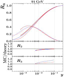
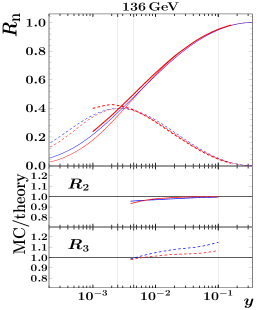
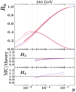
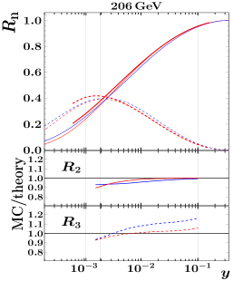
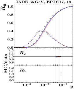
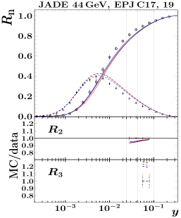
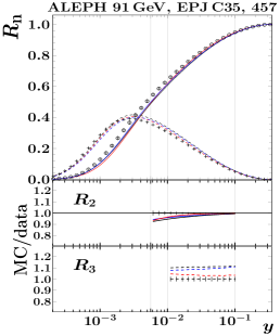
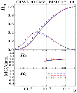
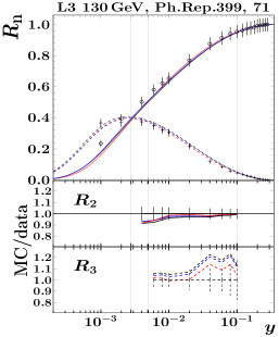
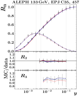
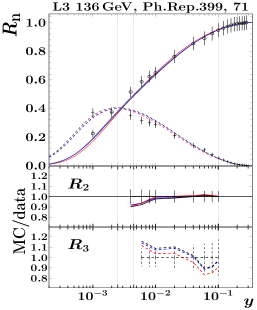
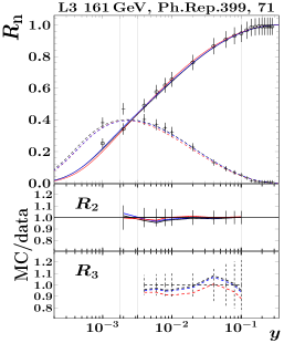
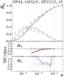
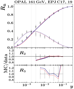
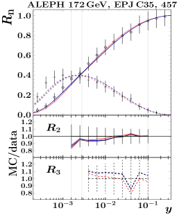
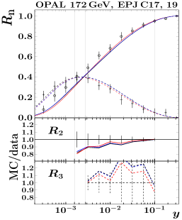
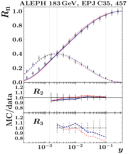
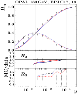
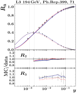
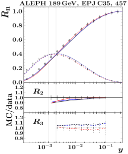
To obtain the jet rates at parton and hadron level, we processed the MC generated samples in the same way as for the data, using undecayed/stable particles for hadron level calculations. To define jets with the Durham clustering, we used the implementation of the FastJet/fjcore3.3.0 package Cacciari:2011ma . The selected resulting distributions are shown in Fig. 8 in Appendix B.

The predictions obtained with all setups describe the data well for all ranges of $y$, with the exception of the regions of small $y$ at all values of $\sqrt{s}$ (see Figs. 9, 10 and 11).

Among all considered MC setups, $H^{L}$ was selected to be the reference. The selected setup uses the very well tested Lund hadronization model that provides stable and physically reliable predictions throughout a wide range of centre-of-mass energies in $e^{+}e^{-}$ collisions. Moreover, precisely this hadronization model was used for the modelling of $e^{+}e^{-}$ collisions in the original publications Pfeifenschneider:1999rz ; Heister:2003aj ; Achard:2004sv .

To estimate the uncertainty related to the hadronization modelling, we consider half the difference between the $H^{L}$ and $H^{C}$ setups, as explained in more detail in the following.

MC generators were already used to model hadronization effects in the previous QCD analyses of $e^{+}e^{-}$ data Kardos:2018kqj ; Dissertori:2007xa . Typically, hadron level predictions for every observable were obtained by multiplying the perturbative predictions by some factor derived from the analysis of MC generated events. In the present analysis the approach was amended to take into account physical constraints on $R_{n}$, namely that jet rates are positive and that their sum should be one. These constraints are implemented by introducing the variables $\xi_{1}$ and $\xi_{2}$ such that at parton level

$$R_{2}^{({\rm p})}=\cos^{2}\xi_{1}\,,\quad R_{3}^{({\rm p})}=\sin^{2}\xi_{1}\cos^{2}\xi_{2}\quad\text{and}\quad R_{\geq 4}^{({\rm p})}=\sin^{2}\xi_{1}\sin^{2}\xi_{2}\,,$$ (9)

with the constraint

$$R_{2}^{({\rm p})}+R_{3}^{({\rm p})}+R_{\geq 4}^{({\rm p})}=1\,.$$ (10)

The corresponding relations at hadron level are

$$R_{2}^{({\rm h})} =\cos^{2}(\xi_{1}+\delta\xi_{1})\,,\quad R_{3}^{({\rm h})}=\sin^{2}(\xi_{1}+\delta\xi_{1})\cos^{2}(\xi_{2}+\delta\xi_{2}),$$

$$R_{\geq 4}^{({\rm h})} =\sin^{2}(\xi_{1}+\delta\xi_{1})\sin^{2}(\xi_{2}+\delta\xi_{2}).$$ (11)

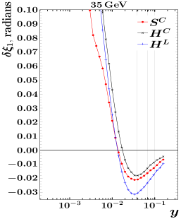
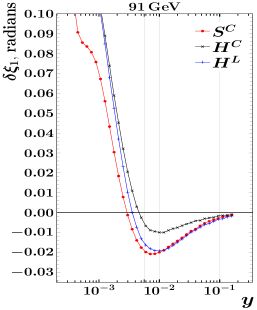
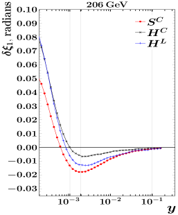
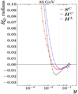
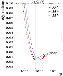
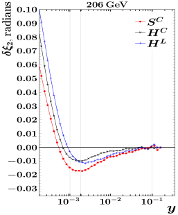
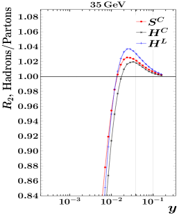
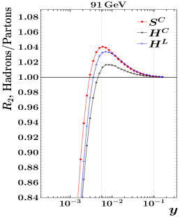
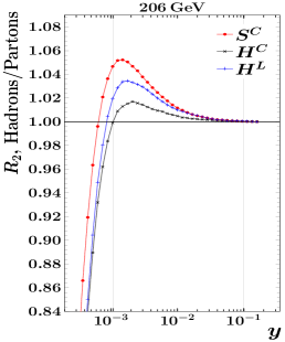
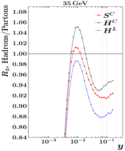
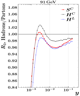
The functions $\delta\xi_{1}(y)$ and $\delta\xi_{2}(y)$ take into account the non-perturbative corrections. We obtained the numerical values for $\delta\xi_{1}(y)$ and $\delta\xi_{2}(y)$ from the MC simulated samples. In order to extract the hadronization corrections we proceed as follows. For a given $y$ bin, we extract $\xi_{1}$ from the parton level prediction for the two-jet rate, and $\xi_{2}$ from the same prediction for the three-jet rate. The shifts $\delta\xi_{1}$ and $\delta\xi_{2}$ are then extracted in the same fashion from the hadron level predictions. The extracted values and corresponding interpolated functions (splines) are shown in Fig. 12 in App. C for selected centre-of-mass energies. The size of the derived hadronization corrections can be read off Fig. 13. As expected, we see that hadronization corrections increase at small values of the two- and three-jet rates and that the corrections become less important at higher energies.

4 Fit procedure

To find the optimal value of $\as$, we used the MINUIT2 minuit package to minimize $\chi^{2}=\sum_{\rm data\ sets}\chi^{2}(\as)_{\rm data\ set},$ where $\chi^{2}(\as)$ was calculated for each data set as

$$\chi^{2}(\as)=\vec{r}\,V^{-1}\,\vec{r}^{T},\qquad\vec{r}\equiv(\vec{D}-\vec{P}(\as)),$$ (12)

where $\vec{D}$ stands for the vector of data points, $\vec{P}(\as)$ is the vector of theoretical predictions, and $V$ is the covariance matrix for the experimental data $\vec{D}$.

We choose the fit range as follows. In order to assure that the implementation of the hadronization corrections is unitary, i.e. the constraint of eq. (10) is satisfied, we set the upper bound of the fit range below the kinematical limit for four jet production, $\log_{10}(y)=\log_{10}(1/6)\simeq-0.8$. We therefore choose $\log_{10}(y)=-1$ as an upper bound. Moreover, we adapt the lower bound to the centre-of-mass energy in order to take into account that hadronization corrections become more important at lower energies. Accordingly, we fix the lower bound $\log_{10}{y_{\rm min}(Q)}$ of the fit range as $\log_{10}{y_{\rm min}(Q)}=\log_{10}{y_{\rm min}}(M_{Z})+{\cal L}$ with ${\cal L}=\log_{10}(M_{Z}^{2}/Q^{2})$. Different values used for $\log_{10}(y_{\rm min}(M_{Z}))$ for $R_{2}$ and $R_{3}$ are indicated in the first columns in Tabs. 2, 4 and 5.

4.1 Fit of the coupling with the two-jet rate $R_{2}$

To obtain the most precise results, we first concentrate on fits that include the two-jet rate $R_{2}$ solely. The results of the fits, together with the used fit ranges, are given in Tab. 2. We show the results obtained via a fit of $R_{2}$ both at N³LO and N³LO+NNLL, with different hadronization models. The corresponding values of $\chi^{2}$ divided by the number of degrees of freedom (${\rm ndof}$) in the global fit is also reported. The values $\chi^{2}/{\rm ndof}$ in the global fit as well as the values for every data set (not shown) are all of order unity, which can be viewed as a support for our correlation model. These values can be compared to the ones obtained in similar analyses. For instance, in Ref. OPAL:2011aa , the $\chi^{2}/{\rm ndof}$ for fits with statistical uncertainties only varies for different observables between $0.5$ and $60$.

From the results given in the table one notices that the effect of the resummation is to move the fitted $\alpha_{s}(M_{Z})$ to slightly lower values. The quality of the fit, with or without resummation, is very similar. The benefit of including the resummation will become evident when perturbative uncertainties of the results are discussed.

Fit ranges, $\log_{10}(y)$	N3LO	N3LO+NNLL
Hadronization	$\chi^{2}/ndof$	$\chi^{2}/ndof$
$[-1.75+{\cal L},-1]$	$0.12121\pm 0.00095$	$0.11849\pm 0.00092$
$S^{C}$	$20/86=0.24$	$20/86=0.24$
$[-2+{\cal L},-1]$	$0.12114\pm 0.00081$	$0.11864\pm 0.00075$
$S^{C}$	$26/100=0.26$	$26/100=0.26$
$[-2.25+{\cal L},-1]$	$0.12119\pm 0.00060$	$0.11916\pm 0.00063$
$S^{C}$	$44/150=0.29$	$44/150=0.29$
$[-2.5+{\cal L},-1]$	$0.12217\pm 0.00052$	$0.12075\pm 0.00055$
$S^{C}$	$89/180=0.50$	$107/180=0.59$
$[-1.75+{\cal L},-1]$	$0.11957\pm 0.00098$	$0.11698\pm 0.00093$
$H^{C}$	$22/86=0.26$	$22/86=0.25$
$[-2+{\cal L},-1]$	$0.11923\pm 0.00079$	$0.11687\pm 0.00076$
$H^{C}$	$29/100=0.29$	$28/100=0.28$
$[-2.25+{\cal L},-1]$	$0.11868\pm 0.00068$	$0.11679\pm 0.00064$
$H^{C}$	$43/150=0.28$	$40/150=0.27$
$[-2.5+{\cal L},-1]$	$0.11849\pm 0.00050$	$0.11723\pm 0.00053$
$H^{C}$	$58/180=0.32$	$58/180=0.32$
$[-1.75+{\cal L},-1]$	$0.12171\pm 0.00109$	$0.11897\pm 0.00092$
$H^{L}$	$21/86=0.25$	$21/86=0.24$
$[-2+{\cal L},-1]$	$0.12144\pm 0.00078$	$0.11893\pm 0.00075$
$H^{L}$	$28/100=0.28$	$26/100=0.26$
$[-2.25+{\cal L},-1]$	$0.12080\pm 0.00069$	$0.11881\pm 0.00063$
$H^{L}$	$43/150=0.28$	$39/150=0.26$
$[-2.5+{\cal L},-1]$	$0.12024\pm 0.00051$	$0.11897\pm 0.00053$
$H^{L}$	$57/180=0.32$	$52/180=0.29$

Table 2: Fit of $\alpha_{s}(M_{Z})$ from experimental data for $R_{2}$ obtained using N³LO and N³LO+NNLL predictions, three different hadronization models and four different choices of the fit range, as given in the brackets, with ${\cal L}=\log_{10}(M_{Z}^{2}/Q^{2})$. The reported uncertainty is the fit uncertainty as given by MINUIT2.

As our best fit we quote the result obtained from the fits of the $R_{2}$ observable with the $H^{L}$ hadronization model in the fit range $[-2.25+{\cal L},-1]$, that reads

$$\as(M_{Z})=0.11881\pm 0.00063{\text{(}exp.)}\pm 0.00101{\text{(}hadr.)}\pm 0.00045{\text{(}ren.)}\pm 0.00034{\text{(}res.)}\,,$$ (13)

where the quoted uncertainties are coming from MINUIT2 $(exp.)$, variation of renormalization scale $(ren.)$, variation of resummation scale $(res.)$ and choice of hadronization model $(hadr.)$. The estimation of these uncertainties is described in the following subsection.

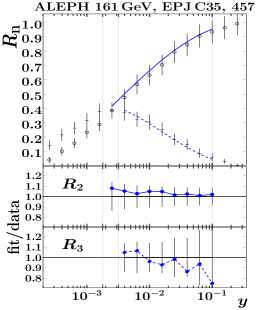
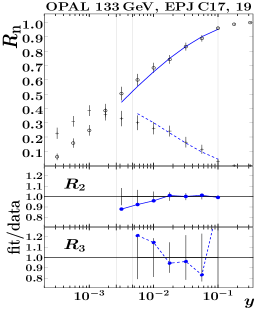
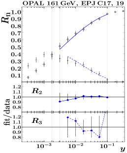
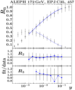
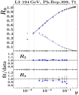
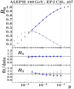
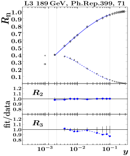
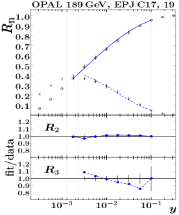
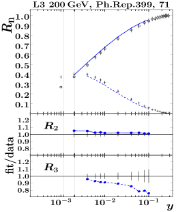
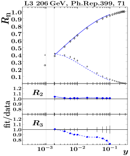
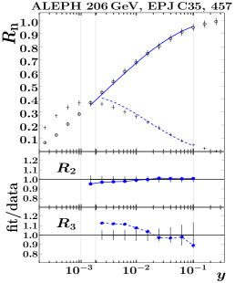
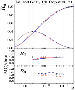
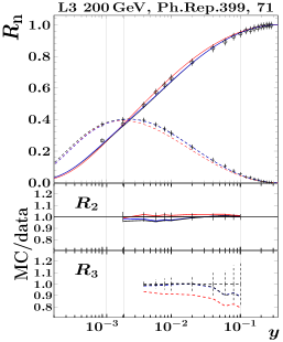
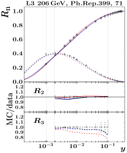
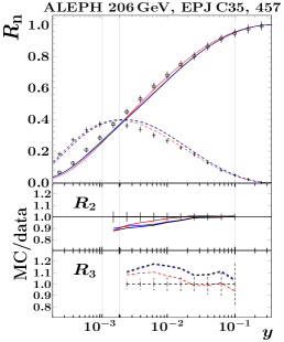
Finally, we show in Figs. 1, 2 and 3 the comparison of data at different energies with theory predictions using $\alpha_{s}(M_{Z})$ obtained from our global fit, eq. (13).

Figure 1: Comparison of data and perturbative predictions supplemented by hadronization corrections in the $H^{L}$ model using for the strong coupling the value obtained from our global fit, eq. (13).

Figure 2: Comparison of data and perturbative predictions supplemented by hadronization corrections in the $H^{L}$ model using for the strong coupling the value obtained from our global fit, eq. (13).

Figure 3: Comparison of data and perturbative predictions supplemented by hadronization corrections in the $H^{L}$ model using for the strong coupling the value obtained from our global fit, eq. (13).

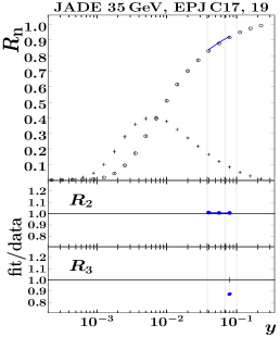
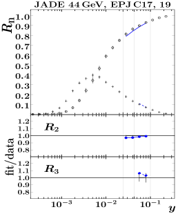
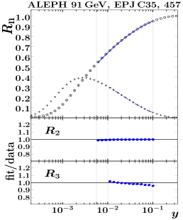
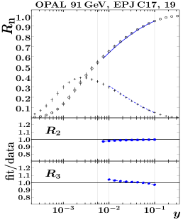
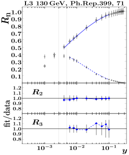
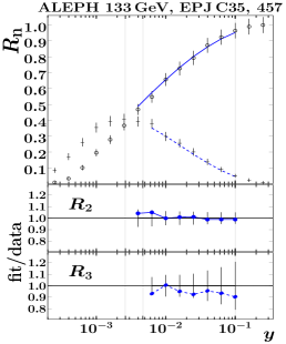
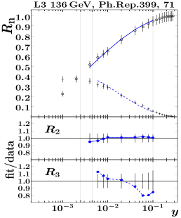
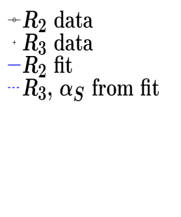
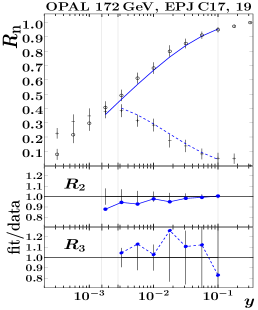
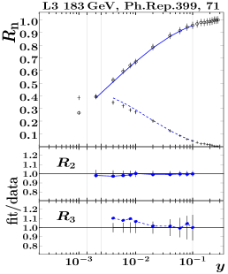
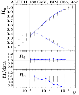
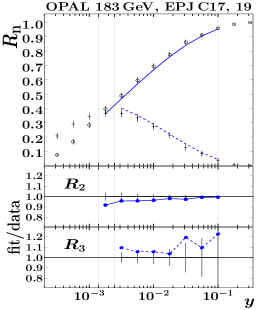
4.2 Estimation of uncertainties

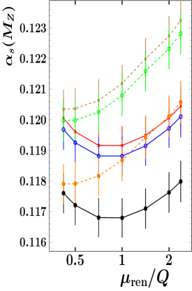
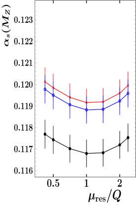
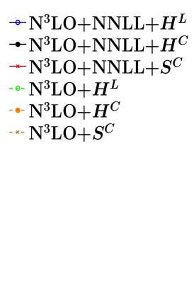
The systematic uncertainties in $\alpha_{s}$ are determined following the procedure of Jones:2003yv . To estimate the size of higher-order terms in the perturbative prediction, we vary the renormalization scale in the range $\mu_{{\rm ren}}=Q/2$ and $\mu_{{\rm ren}}=2Q$. Moreover, while keeping $\mu_{{\rm ren}}=Q$ fixed, we vary the resummation scale in the range $\mu_{{\rm res}}=Q/2$ and $\mu_{{\rm res}}=2Q$. The effects of the individual variations are displayed in Fig. 4, where different hadronization models are compared. We notice that, when resummation is included, a much reduced dependence on the renormalization scale is observed.

The bias due to the selection of the hadronization model is studied by means of the difference between the $H^{L}$ and $H^{C}$ setups, see Fig. 4. In particular, considering the results from the Lund string and cluster hadronization models, the desired systematic uncertainty is obtained as half of the difference between the $\alpha_{S}(M_{Z})$ results obtained in nominal fits with $H^{L}$ and $H^{C}$ setups. The obtained numerical value is close to $0.001$ (i.e. slightly below 1%). This can be briefly compared to previous estimations obtained with Monte Carlo event generator models in similar analyses. Namely, the values $0.001$ Dissertori:2007xa ; OPAL:2011aa and $0.0005$ Dissertori:2009ik obtained previously allow us to validate our estimation. We stress that we have not performed any tuning of the adopted hadronization models to the data in order to artificially reduce the related uncertainties. This leads to a more conservative, and thus more robust estimate of hadronization uncertainties.

The final uncertainty is obtained by combining each of the above uncertainties in quadrature.

Figure 4: Dependence of ($R_{2}$) fit results on the renormalization and resummation scales. The fit range for $S^{C}$, $H^{C}$ and $H^{L}$ setups is $[-2.25+{\cal L},-1]$ with ${\cal L}=\log_{10}(M_{Z}^{2}/Q^{2})$.

5 Validation of the procedure and further fits

In this section we perform some consistency checks to validate the fitting procedure used above. Moreover, we present an extraction of $\alpha_{s}(M_{Z})$ from a simultaneous fit of $R_{2}$ at N³LO+NNLL and $R_{3}$ at NNLO.

5.1 Fit consistency tests

We have performed a number of consistency tests, as outlined in the following:

1. We repeat the nominal fits in different ranges of $\sqrt{s}$ separately, instead of simultaneously. The results of these fits are shown in Fig. 5. We do not observe any significant dependence of the results on the centre-of-mass energy.

   

   

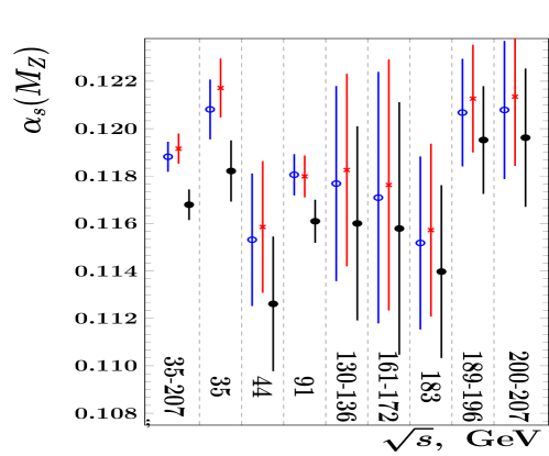
   Figure 5: Dependence of ($R_{2}$) fit results on the $\sqrt{s}$ of measurement. The fit range is $[-2.25+{\cal L},-1]$. Only statistical uncertainties are shown.

2. We repeat the nominal fit for $R_{2}$ by implementing the hadronization corrections on a bin-by-bin basis as $R_{2,{\rm hadron}}=R_{2,{\rm parton}}f_{2}(y)$, where $f_{2}(y)$ is derived from the MC generated samples. Within this scheme, we find

   $\as(M_{Z})=0.11881\pm 0.00063{\text{(}exp.)}\pm 0.00109{\text{(}hadr.)}.$

   This value is close to the reference result, but the hadronization uncertainty estimated from this setup is more sensitive to changes in the fit range.

3. To test the reliability of the correlation model used for the systematic uncertainties in the reference fit, we use the OPAL data and systematic shifts (uncertainties) from Ref. Verbytskyi201813 . With this data we perform the fits using the $\chi^{2}$ definition from eq. (12) and the definition that explicitly includes set of $N$ nuisance parameters $B=\{b_{1},b_{2}\dots b_{N}\}$ and vectors of systematic shifts (uncertainties) $\vec{S_{1}},\vec{S_{2}}\dots\vec{S_{N}}$:

   $$\chi^{2}(\as,B)=(\vec{r}-\sum_{i=1}^{N}b_{i}\vec{S_{i}})V^{-1}(\vec{r}-\sum_{i=1}^{N}b_{i}\vec{S_{i}})^{T}+\sum_{i=1}^{N}b_{i}^{2}.$$ (14)

   The result is

   $\as(M_{Z})=0.11893\pm 0.00137{\text{(}exp.)}$ for the definition in eq. (12)

   and

   $\as(M_{Z})=0.11761\pm 0.00179{\text{(}exp.)}$ for the definition in eq. (14).

   These results are in fair agreement, and the corresponding values of $\chi^{2}$ are close, which demonstrates the relatively good performance of the selected correlation model.

4. We repeat the reference fit without the data sets from JADE, for which the explicit verification of correlation model using Ref. Verbytskyi201813 was not possible. The obtained result $\as(M_{Z})=0.11838\pm 0.00077{\text{(}exp.)}$ agrees well with the reference value $\as(M_{Z})=0.11881\pm 0.00063{\text{(}exp.)}\pm 0.00101{\text{(}hadr.)}\pm 0.00045{\text{(}ren.)}\pm 0.00034{\text{(}res.)}$.

5. To estimate the error due to the correlation model, we vary the value of the parameter $\rho$ in a wide range. No significant change of fit results was observed, see Fig. 6.

   

   

   

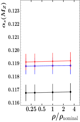
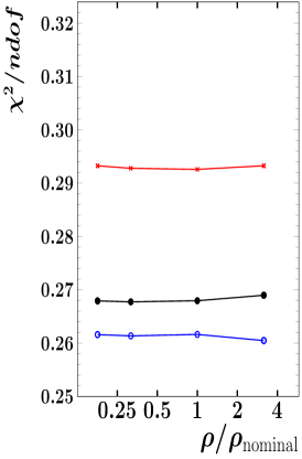
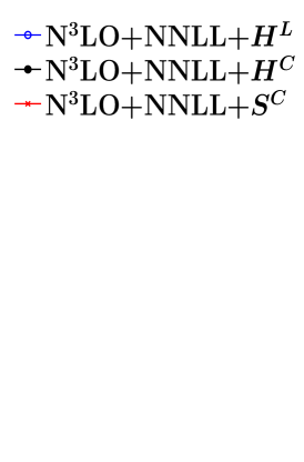
   Figure 6: Dependence of the ($R_{2}$) fit results on the parameter $\rho$ used in the correlation model. The fit range is fixed to $[-2.25+{\cal L},-1]$.

6. We perform variations of the renormalization and resummation scales simultaneously, as done in Ref. Schieck:2012mp . The results are reported in Fig. 7 and show smaller uncertainty than in the case of independent variations.

   

   

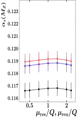
   Figure 7: Dependence of the ($R_{2}$) fit results on the simultaneous variation of renormalization and resummation scales. The fit range is fixed to $[-2.25+{\cal L},-1]$.

   A similar behaviour was observed in Ref. Kardos:2018kqj .

5.2 Simultaneous fit of the coupling with the two- and three- jet rates $R_{2}$ and $R_{3}$

An alternative fit was performed with $R_{2}$ and $R_{3}$ observables simultaneously, with $R_{3}$ computed at NNLO. The obtained result using the $[-2.25+{\cal L},-1][-2+{\cal L},-1]$ fit ranges for $R_{2}$ and $R_{3}$, respectively, and the $H^{L}$ setup is

$\as(M_{Z})=0.11989\pm 0.00045{\text{(}exp.)}\pm 0.00098{\text{(}hadr.)}\pm 0.00046{\text{(}ren.)}\pm 0.00017{\text{(}res.)}.$

Unlike the results of the reference fits, the obtained result is sensitive to the selected fit range, see Tab. 4 in App. D. Taking this effect into account would result in another uncertainty of order $0.001$ that is not included in the uncertainties given above.

As a final cross-check we perform a fit for a single point of ALEPH $R_{3}$ data at $y=0.02$ without resummation. The obtained result (with statistical uncertainties only), $\as(M_{Z})=0.11905\pm 0.00251{\text{(}exp.)}$, can be compared to the results from Ref. Dissertori:2009qa , $\as(M_{Z})=0.1175\pm 0.0020{\text{(}exp.)}\pm 0.0015{\text{(}theo.)}$. The results agree well despite the differences in the implementation of the hadronization corrections.

5.3 Discussion

The value obtained from the analysis relying on N³LO+NNLL predictions for $R_{2}$ is in agreement with the world average as of 2017 Bethke:2017uli , however it is visibly lower than the results from measurements performed for other $e^{+}e^{-}$ observables using NNLO perturbative QCD predictions and MC hadronization models Bethke:2017uli . The estimated uncertainties are on the other hand approximately of the same sizes.

6 Summary

The main result of this paper is a first fit of the strong coupling for the two-jet rate that relies on very accurate (N³LO+NNLL) predictions. Our main result reads

$$\as(M_{Z})=0.11881\pm 0.00063{\text{(}exp.)}\pm 0.00101{\text{(}hadr.)}\pm 0.00045{\text{(}ren.)}\pm 0.00034{\text{(}res.)}.$$

The uncertainty on $\alpha_{s}$ induced by scale variations is now considerably smaller than that related to hadronization modelling. This is not the case if the fit is performed using only N³LO predictions, see Fig. 4. Furthermore the experimental uncertainty is now comparable to the perturbative one.

After combining the uncertainties in quadrature we obtain

$$\as(M_{Z})=0.11881\pm 0.00131{\text{(}comb.)},$$

where the largest estimation bias comes from the used hadronization model.

Our results agrees with the last PDG average

$$\as(M_{Z})_{\rm PDG2018}=0.1181\pm 0.0011$$

with an uncertainty that is of the same size.

We have also performed a combined fit of the two- and three-jet rate, taking for the first time the correlation between these observables into account. The results of the two fits are fully compatible. However, the fit including $R_{3}$ shows a stronger dependence on the fit range than the results of our reference fit based on $R_{2}$ only. An accurate resummation for the $R_{3}$ observable could potentially reduce the sensitivity to the fit range selection and lead to an even more precise determination of $\as(M_{Z})$.

Appendix A Perturbative ingredients

We report in Tab. 3 the numerical results for the fixed-order coefficients introduced in eq. (5).

$y$	$A_{3}$	$A_{4}$	$A_{5}$	$B_{3}$	$B_{4}$	$C_{3}$
0.000249	64.853	2226.9	52659	-2276.3	-18059	-52708
0.000304	61.462	1981.9	43613	-1951.9	-9434	-49312
0.000371	57.969	1745.7	35503	-1644.5	-2392	-45862
0.000453	54.589	1531.6	28680	-1370.8	2875.1	-41808
0.000553	51.315	1337.6	22984	-1126.4	6726.2	-38197
0.000676	48.149	1162.6	18248	-911.38	9293.8	-33891
0.000825	45.081	1005.5	14362	-722.69	10902	-29909
0.001008	42.125	864.92	11185	-558.20	11665	-25860
0.001231	39.267	739.71	8612	-416.39	11905	-22437
0.001503	36.514	628.56	6548	-295.16	11595	-18881
0.001836	33.865	530.39	4910	-192.34	10949	-15681
0.002243	31.318	444.20	3627	-106.70	10084	-12771
0.002739	28.874	368.93	2634	-36.132	9080.6	-10373
0.003346	26.532	303.65	1875	20.7909	8018.6	-8011
0.004087	24.292	247.42	1307	65.2347	6936.3	-6144
0.004992	22.155	199.36	888.5	98.9217	5886.0	-4478
0.006097	20.118	158.62	586.9	123.332	4897.6	-3090
0.007447	18.183	124.43	374.8	139.397	3982.9	-1863
0.009095	16.354	96.058	230.1	148.398	3173.8	-944.6
0.011109	14.621	72.787	134.4	151.554	2469.0	-218.7
0.013569	12.988	53.978	74.07	149.800	1868.4	250.42
0.016573	11.455	39.019	37.89	144.067	1373.2	580.39
0.020242	10.019	27.368	17.63	135.256	974.01	724.38
0.024724	8.6830	18.495	7.213	124.148	662.70	917.46
0.030197	7.4420	11.934	2.471	111.328	428.24	950.16
0.036883	6.2962	7.2589	0.647	97.6721	260.70	897.90
0.045049	5.2435	4.0822	0.110	83.5664	145.88	812.72
0.055023	4.2842	2.0589	0.008	69.5476	73.141	700.85
0.067206	3.4173	0.8849	0.000	56.1021	31.186	571.07
0.082085	2.6424	0.2950	-0.00	43.4943	10.302	449.83
0.100259	1.9584	0.0630	-0.00	32.1309	2.1788	326.17
0.122456	1.3647	0.0056	0.000	22.1977	0.1915	218.79
0.149569	0.8612	0.0000	0.000	13.8521	0.0005	133.14
0.182684	0.4500	-0.000	0.000	7.16729	-0.000	73.647
0.223130	0.1366	0.0000	-0.00	2.15434	0.0000	24.828
0.272532	0.1320	-0.000	0.000	2.08088	0.0000	23.734

Table 3: The perturbative coefficients entering eq. (5) as calculated by the MCCSM program.

Appendix B MC simulations at hadron and parton levels

The figures in this section contain data measurements and predictions for jet rates calculated in very fine binning at parton (Fig. 8) and hadron (Figs. 9, 10 and  11) levels using different MC setups. The plots with ratios of hadron level predictions to data measurements are calculated with the binning used in the measurements. The error bars in the plots are calculated from the total uncertainty of the data points. The vertical lines in the plots show the fit ranges used in this work for fits of the $R_{2}$ and $R_{3}$ observables.

Figure 8: Selected predictions obtained with $S^{C}$, $H^{C}$ and $H^{L}$ MC setups at parton level and theory predictions obtained with $\alpha_{S}(M_{Z})=0.1181$.

Figure 9: Predictions obtained with $S^{C}$, $H^{C}$ and $H^{L}$ MC setups at hadron level.

Figure 10: Predictions obtained with $S^{C}$, $H^{C}$ and $H^{L}$ MC setups at hadron level.

Figure 11: Predictions obtained with $S^{C}$, $H^{C}$ and $H^{L}$ MC setups at hadron level.

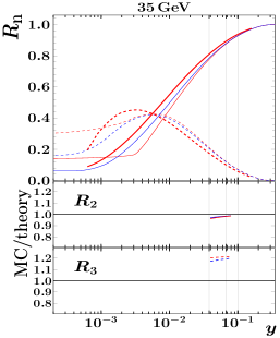
Appendix C Hadronization corrections

Fig. 12 shows the $\delta\xi_{1}$ and $\delta\xi_{2}$ distributions used to model hadronization corrections of jet rates at different centre-of-mass energies. As before, the vertical lines in the plots show the fit range for reference fits of the $R_{2}$ and $R_{3}$ observables. Fig. 13 shows the size of hadronization corrections obtained from the $\delta\xi_{1}$ and $\delta\xi_{2}$ values using eqs. (9) and (11).

Figure 12: Hadronization corrections obtained with $S^{C}$, $H^{C}$ and $H^{L}$ hadronization models.

Figure 13: Hadronization corrections obtained with $S^{C}$, $H^{C}$ and $H^{L}$ hadronization models.

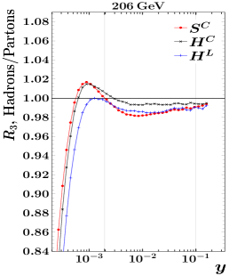
Appendix D Additional fits

In this section we present results of additional fits that we have performed.

Table 4 shows a simultaneous fit of $\alpha_{s}(M_{Z})$ from experimental data for $R_{2}$ and $R_{3}$ obtained using N³LO and N³LO+NNLL predictions for $R_{2}$ and NNLO predictions for $R_{3}$. Three different hadronization models are used and four different choices of the fit range are shown. The reported uncertainty is only the statistical uncertainty of the fit, as given by MINUIT2. We note that these results show a significant dependence on the fit range used.

Fit ranges, $\log y$	N3LO, NNLO	N3LO+NNLL, NNLO
Hadronization	$\chi^{2}/ndof$	$\chi^{2}/ndof$
$[-1.75+{\cal L},-1][-1.5+{\cal L},-1]$	$0.12195\pm 0.00072$	$0.12078\pm 0.00066$
$S^{C}$	$120/143=0.84$	$140/143=0.98$
$[-2+{\cal L},-1][-1.75+{\cal L},-1]$	$0.12163\pm 0.00061$	$0.12065\pm 0.00056$
$S^{C}$	$153/187=0.82$	$176/187=0.94$
$[-2.25+{\cal L},-1][-2+{\cal L},-1]$	$0.12075\pm 0.00044$	$0.11994\pm 0.00041$
$S^{C}$	$208/251=0.83$	$222/251=0.88$
$[-2.5+{\cal L},-1][-2.25+{\cal L},-1]$	$0.12143\pm 0.00043$	$0.12089\pm 0.00044$
$S^{C}$	$321/331=0.97$	$336/331=1.01$
$[-1.75+{\cal L},-1][-1.5+{\cal L},-1]$	$0.12068\pm 0.00073$	$0.11956\pm 0.00066$
$H^{C}$	$126/143=0.88$	$147/143=1.03$
$[-2+{\cal L},-1][-1.75+{\cal L},-1]$	$0.12006\pm 0.00061$	$0.11913\pm 0.00054$
$H^{C}$	$163/187=0.87$	$188/187=1.01$
$[-2.25+{\cal L},-1][-2+{\cal L},-1]$	$0.11869\pm 0.00043$	$0.11793\pm 0.00043$
$H^{C}$	$221/251=0.88$	$238/251=0.95$
$[-2.5+{\cal L},-1][-2.25+{\cal L},-1]$	$0.11845\pm 0.00045$	$0.11799\pm 0.00047$
$H^{C}$	$302/331=0.91$	$310/331=0.94$
$[-1.75+{\cal L},-1][-1.5+{\cal L},-1]$	$0.12248\pm 0.00068$	$0.12129\pm 0.00063$
$H^{L}$	$121/143=0.85$	$141/143=0.99$
$[-2+{\cal L},-1][-1.75+{\cal L},-1]$	$0.12211\pm 0.00057$	$0.12110\pm 0.00053$
$H^{L}$	$155/187=0.83$	$180/187=0.96$
$[-2.25+{\cal L},-1][-2+{\cal L},-1]$	$0.12071\pm 0.00044$	$0.11989\pm 0.00045$
$H^{L}$	$209/251=0.83$	$227/251=0.90$
$[-2.5+{\cal L},-1][-2.25+{\cal L},-1]$	$0.12041\pm 0.00044$	$0.11990\pm 0.00044$
$H^{L}$	$266/331=0.80$	$278/331=0.84$

Table 4: Simultaneous fit of $\alpha_{s}(M_{Z})$ from experimental data for $R_{2}$ and $R_{3}$ obtained using N³LO and N³LO+NNLL predictions for $R_{2}$ and NNLO predictions for $R_{3}$. Three different hadronization models are used and four different choices of the fit range are shown, as given in the brackets, with ${\cal L}=\log_{10}(M_{Z}^{2}/Q^{2})$. The fit range for $R_{2}$ is given in the first pair of brackets and the the fit range for $R_{3}$ in the second. The reported uncertainty is the fit uncertainty only, as given by MINUIT2.

We also show in Tab. 5 a fit of $\alpha_{s}(M_{Z})$ from experimental data for $R_{3}$ only obtained using NNLO predictions, three different hadronization models and four different choices of the fit range. As before, the reported uncertainty is the fit uncertainty only, as given by MINUIT2. These results can be compared directly with results of similar analyses, such as the study of Ref. Dissertori:2009qa . Altogether we find good agreement between the fitted values reported in Tab. 5 and the results of Ref. Dissertori:2009qa .

Fit ranges, $\log y$	NNLO
Hadronization	$\chi^{2}/ndof$
$[-1.5+{\cal L},-1]$	$0.12176\pm 0.00113$
$S^{C}$	$39/56=0.70$
$[-1.75+{\cal L},-1]$	$0.12088\pm 0.00088$
$S^{C}$	$56/86=0.65$
$[-2+{\cal L},-1]$	$0.11996\pm 0.00074$
$S^{C}$	$74/100=0.74$
$[-2.25+{\cal L},-1]$	$0.11853\pm 0.00068$
$S^{C}$	$111/150=0.74$
$[-1.5+{\cal L},-1]$	$0.12053\pm 0.00114$
$H^{C}$	$41/56=0.74$
$[-1.75+{\cal L},-1]$	$0.11933\pm 0.00084$
$H^{C}$	$61/86=0.70$
$[-2+{\cal L},-1]$	$0.11810\pm 0.00074$
$H^{C}$	$83/100=0.83$
$[-2.25+{\cal L},-1]$	$0.11645\pm 0.00061$
$H^{C}$	$125/150=0.83$
$[-1.5+{\cal L},-1]$	$0.12257\pm 0.00112$
$H^{L}$	$39/56=0.70$
$[-1.75+{\cal L},-1]$	$0.12178\pm 0.00088$
$H^{L}$	$57/86=0.66$
$[-2+{\cal L},-1]$	$0.12076\pm 0.00068$
$H^{L}$	$75/100=0.75$
$[-2.25+{\cal L},-1]$	$0.11931\pm 0.00067$
$H^{L}$	$115/150=0.77$

Table 5: Fit of $\alpha_{s}(M_{Z})$ from experimental data for $R_{3}$ obtained using NNLO predictions, three different hadronization models and four different choices of the fit range, as given in the brackets, where ${\cal L}=\log_{10}(M_{Z}^{2}/Q^{2})$. The reported uncertainty is the fit uncertainty only, as given by MINUIT2.

References

- (1) H. Fritzsch, M. Gell-Mann and H. Leutwyler, Advantages of the color octet gluon picture, Phys. Lett. B47 (1973) 365.
- (2) D.J. Gross and F. Wilczek, Ultraviolet behavior of nonabelian gauge theories, Phys. Rev. Lett. 30 (1973) 1343.
- (3) H. Politzer, Reliable perturbative results for strong interactions?, Phys. Rev. Lett. 30 (1973) 1346.
- (4) D.J. Gross and F. Wilczek, Asymptotically free gauge theories. 1, Phys. Rev. D8 (1973) 3633.
- (5) Particle Data Group collaboration, Review of Particle Physics, Chin. Phys. C40 (2016) 100001.
- (6) Y.L. Dokshitzer, G. Marchesini and B.R. Webber, Dispersive approach to power behaved contributions in QCD hard processes, Nucl. Phys. B469 (1996) 93 [hep-ph/9512336].
- (7) A. Gehrmann-De Ridder et al., NNLO corrections to event shapes in annihilation, JHEP 12 (2007) 094 [0711.4711].
- (8) A. Gehrmann-De Ridder et al., Jet rates in electron-positron annihilation at in QCD, Phys. Rev. Lett. 100 (2008) 172001 [0802.0813].
- (9) S. Weinzierl, NNLO corrections to 3-jet observables in electron-positron annihilation, Phys. Rev. Lett. 101 (2008) 162001 [0807.3241].
- (10) S. Weinzierl, Event shapes and jet rates in electron-positron annihilation at NNLO, JHEP 06 (2009) 041 [0904.1077].
- (11) V. Del Duca et al., Jet production in the CoLoRFulNNLO method: event shapes in electron-positron collisions, Phys. Rev. D94 (2016) 074019 [1606.03453].
- (12) S.G. Gorishnii, A.L. Kataev and S.A. Larin, The -corrections to and in QCD, Phys. Lett. B259 (1991) 144.
- (13) T. Becher and M. Schwartz, A precise determination of from LEP thrust data using effective field theory, JHEP 07 (2008) 034 [0803.0342].
- (14) R. Abbate et al., Thrust at LL with power corrections and a precision global fit for , Phys.Rev. D83 (2011) 074021 [1006.3080].
- (15) P.F. Monni, T. Gehrmann and G. Luisoni, Two-Loop Soft Corrections and Resummation of the Thrust Distribution in the Dijet Region, JHEP 08 (2011) 010 [1105.4560].
- (16) T. Becher and G. Bell, NNLL Resummation for jet broadening, JHEP 1211 (2012) 126 [1210.0580].
- (17) A. Hoang et al., -parameter distribution at N3LL including power corrections, Phys. Rev. D91 (2015) 094017 [1411.6633].
- (18) D. de Florian and M. Grazzini, The back-to-back region in energy-energy correlation, Nucl. Phys. B704 (2005) 387 [hep-ph/0407241].
- (19) A. Banfi et al., A general method for the resummation of event-shape distributions in annihilation, JHEP 1505 (2015) 102 [1412.2126].
- (20) A. Banfi et al., The two-jet rate in at next-to-next-to-leading-logarithmic order, Phys. Rev. Lett. 117 (2016) 172001 [1607.03111].
- (21) Z. Tulipánt, A. Kardos and G. Somogyi, Energy-energy correlation in electron–positron annihilation at NNLL + NNLO accuracy, Eur. Phys. J. C77 (2017) 749 [1708.04093].
- (22) I. Moult and H.X. Zhu, Simplicity from Recoil: The Three-Loop Soft Function and Factorization for the Energy-Energy Correlation, JHEP 08 (2018) 160 [1801.02627].
- (23) A. Banfi, B.K. El-Menoufi and P.F. Monni, The Sudakov radiator for jet observables and the soft physical coupling, 1807.11487.
- (24) G. Bell et al., angularity distributions at NNLL′ accuracy, 1808.07867.
- (25) T. Gehrmann, G. Luisoni and P.F. Monni, Power corrections in the dispersive model for a determination of the strong coupling constant from the thrust distribution, Eur. Phys. J. C73 (2013) 2265 [1210.6945].
- (26) A. Kardos et al., Precise determination of from a global fit of energy–energy correlation to NNLO+NNLL predictions, Eur. Phys. J. C78 (2018) 498 [1804.09146].
- (27) S. Catani et al., New clustering algorithm for multi-jet cross-sections in annihilation, Phys. Lett. B269 (1991) 432.
- (28) G. Somogyi, Z. Trócsányi and V. Del Duca, A Subtraction scheme for computing QCD jet cross sections at NNLO: Regularization of doubly-real emissions, JHEP 01 (2007) 070 [hep-ph/0609042].
- (29) G. Somogyi and Z. Trócsányi, A Subtraction scheme for computing QCD jet cross sections at NNLO: Regularization of real-virtual emission, JHEP 01 (2007) 052 [hep-ph/0609043].
- (30) A. Kardos, G. Somogyi and Z. Trócsányi, Jet cross sections with CoLoRFul NNLO, PoS LL2016 (2016) 021.
- (31) A. Banfi, G.P. Salam and G. Zanderighi, Semi-numerical resummation of event shapes, JHEP 01 (2002) 018 [hep-ph/0112156].
- (32) S. Catani et al., Resummation of large logarithms in event shape distributions, Nucl. Phys. B407 (1993) 3.
- (33) P. Nason and C. Oleari, Next-to-leading order corrections to momentum correlations in , Phys. Lett. B407 (1997) 57 [hep-ph/9705295].
- (34) F. Krauss and G. Rodrigo, Resummed jet rates for annihilation into massive quarks, Phys. Lett. B576 (2003) 135 [hep-ph/0303038].
- (35) K.G. Chetyrkin, R.V. Harlander and J.H. Kühn, Quartic mass corrections to at order , Nucl.Phys. B586 (2000) 56 [hep-ph/0005139].
- (36) P. Nason and C. Oleari, Next-to-leading order corrections to the production of heavy flavor jets in collisions, Nucl. Phys. B521 (1998) 237 [hep-ph/9709360].
- (37) OPAL collaboration, Test of the flavor independence of alpha(s) using next-to-leading order calculations for heavy quarks, Eur. Phys. J. C11 (1999) 643 [hep-ex/9904013].
- (38) K. G. Chetyrkin, J. H. Kuhn and M. Steinhauser, RunDec: A Mathematica package for running and decoupling of the strong coupling and quark masses, Comput. Phys. Commun. 133 (2000) 43 [hep-ph/0004189].
- (39) Particle Data Group collaboration, Review of Particle Physics, Phys. Rev. D98 (2018) 030001.
- (40) ALEPH Collaboration collaboration, Properties of hadronic decays and test of QCD generators, Z. Phys. C55 (1992) 209.
- (41) OPAL Collaboration collaboration, QCD studies with annihilation data at , Z. Phys. C75 (1997) 193.
- (42) OPAL Collaboration collaboration, QCD studies with annihilation data at and , Z. Phys. C72 (1996) 191.
- (43) JADE and OPAL Collaborations collaboration, QCD analyses and determinations of in annihilation at energies between and , Eur. Phys. J. C17 (2000) 19 [hep-ex/0001055].
- (44) OPAL Collaboration collaboration, A global determination of at LEP, Z. Phys. C55 (1992) 1.
- (45) JADE Collaboration collaboration, Measurement of the strong coupling from the three-jet rate in - annihilation using JADE data, Eur. Phys. J. C73 (2013) 2332 [1205.3714].
- (46) L3 Collaboration collaboration, Studies of hadronic event structure in annihilation from to with the L3 detector, Phys. Rept. 399 (2004) 71 [hep-ex/0406049].
- (47) DELPHI Collaboration collaboration, Measurement of event shape and inclusive distributions at and , Z. Phys. C73 (1997) 229.
- (48) ALEPH Collaboration collaboration, Studies of QCD at centre-of-mass energies between and , Eur. Phys. J. C35 (2004) 457.
- (49) OPAL Collaboration collaboration, A study of the recombination scheme dependence of jet production rates and of in hadronic decays, Z. Phys. C49 (1991) 375.
- (50) L3 Collaboration collaboration, QCD studies and determination of in collisions at and , Phys. Lett. B404 (1997) 390.
- (51) A. Verbytskyi, Studies of correlations between measurements of jet observables, JINST 12 (2017) P04013 [1609.06898].
- (52) A. Verbytskyi, Measurements of durham, anti- and SIScone jet rates at LEP with the OPAL detector, Nuclear and Particle Physics Proceedings 294-296 (2018) 13.
- (53) J. Bellm et al., Herwig 7.0/Herwig++ 3.0 release note, Eur. Phys. J. C76 (2016) 196 [1512.01178].
- (54) T. Gleisberg et al., Event generation with SHERPA 1.1, JHEP 02 (2009) 007 [0811.4622].
- (55) S. Plätzer, Controlling inclusive cross sections in parton shower + matrix element merging, JHEP 08 (2013) 114 [1211.5467].
- (56) J. Alwall et al., MadGraph 5 : Going Beyond, JHEP 06 (2011) 128 [1106.0522].
- (57) F. Cascioli, P. Maierhofer and S. Pozzorini, Scattering Amplitudes with Open Loops, Phys. Rev. Lett. 108 (2012) 111601 [1111.5206].
- (58) B. Webber, A QCD model for jet fragmentation including soft gluon interference, Nucl. Phys. B238 (1984) 492.
- (59) B. Andersson et al., Parton Fragmentation and String Dynamics, Phys. Rept. 97 (1983) 31.
- (60) T. Sjöstrand, S. Mrenna and P.Z. Skands, A brief introduction to PYTHIA 8.1, Comput. Phys. Commun. 178 (2008) 852 [0710.3820].
- (61) L. Lönnblad, ThePEG, Pythia7, herwig++ and Ariadne, Nucl. Instrum. Meth. A559 (2006) 246.
- (62) D.J. Lange, The EvtGen particle decay simulation package, Nucl. Instrum. Meth. A462 (2001) 152.
- (63) F. Krauss, R. Kuhn and G. Soff, AMEGIC++ 1.0: A Matrix element generator in C++, JHEP 02 (2002) 044 [hep-ph/0109036].
- (64) C. Duhr, S. Hoeche and F. Maltoni, Color-dressed recursive relations for multi-parton amplitudes, JHEP 08 (2006) 062 [hep-ph/0607057].
- (65) J.C. Winter, F. Krauss and G. Soff, A modified cluster hadronization model, Eur. Phys. J. C36 (2004) 381 [hep-ph/0311085].
- (66) M. Cacciari, P.G. Salam and G. Soyez, FastJet user manual, Eur. Phys. J. C72 (2012) 1896 [1111.6097].
- (67) G. Dissertori et al., First determination of the strong coupling constant using NNLO predictions for hadronic event shapes in annihilations, JHEP 02 (2008) 040 [0712.0327].
- (68) F. James and M. Roos, Minuit: A system for function minimization and analysis of the parameter errors and correlations, Comput.Phys.Commun. 10 (1975) 343.
- (69) OPAL Collaboration collaboration, Determination of using OPAL hadronic event shapes at and resummed NNLO calculations, Eur. Phys. J. C71 (2011) 1733 [1101.1470].
- (70) R.W.L. Jones et al., Theoretical uncertainties on from event shape variables in annihilations, JHEP 12 (2003) 007 [hep-ph/0312016].
- (71) G. Dissertori et al., Determination of the strong coupling constant using matched NNLO+NLLA predictions for hadronic event shapes in annihilations, JHEP 08 (2009) 036 [0906.3436].
- (72) S. Alekhin et al., HERAFitter, Eur. Phys. J. C75 (2015) 304 [1410.4412].
- (73) G. Dissertori et al., Precise determination of the strong coupling constant at NNLO in QCD from the three-jet rate in electron-positron annihilation at LEP, Phys. Rev. Lett. 104 (2010) 072002 [0910.4283].
- (74) S. Bethke, 2016, Nucl. Part. Phys. Proc. 282-284 (2017) 149.