A Nonparametric Multi-view Model for Estimating
Cell Type-Specific Gene Regulatory Networks

Abstract

We present a Bayesian hierarchical multi-view mixture model termed Symphony that simultaneously learns clusters of cells representing cell types and their underlying gene regulatory networks by integrating data from two views: single-cell gene expression data and paired epigenetic data, which is informative of gene-gene interactions. This model improves interpretation of clusters as cell types with similar expression patterns as well as regulatory networks driving expression, by explaining gene-gene covariances with the biological machinery regulating gene expression. We show the theoretical advantages of the multi-view learning approach and present a Variational EM inference procedure. We demonstrate superior performance on both synthetic data and real genomic data with subtypes of peripheral blood cells compared to other methods.

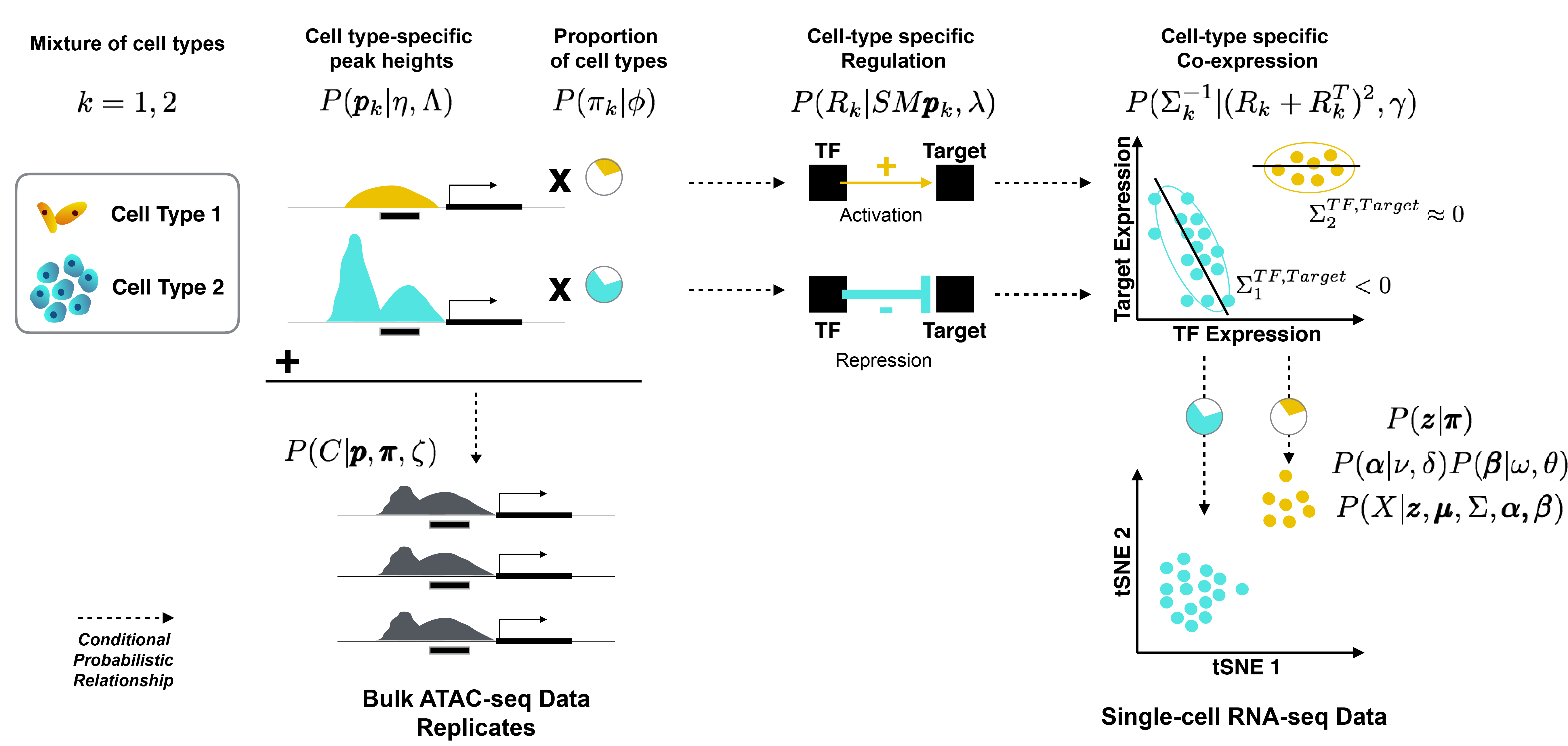
Figure 1: The generative process in Symphony: We aim to infer gene regulatory networks (GRNs) denoted as $R_{k}$ specific to each cluster of cells from integration of two views: Epigenetic data (indicative of network edges) from the bulk of cells ($C$) and expression of genes (network nodes) at resolution of single cells ($X$). GRNs are directed weighted networks with edge weights denoting regulatory impact of one gene on another (e.g. activation or repression); the impact of regulation is reflected in covariance between genes ($\Sigma_{k}$).

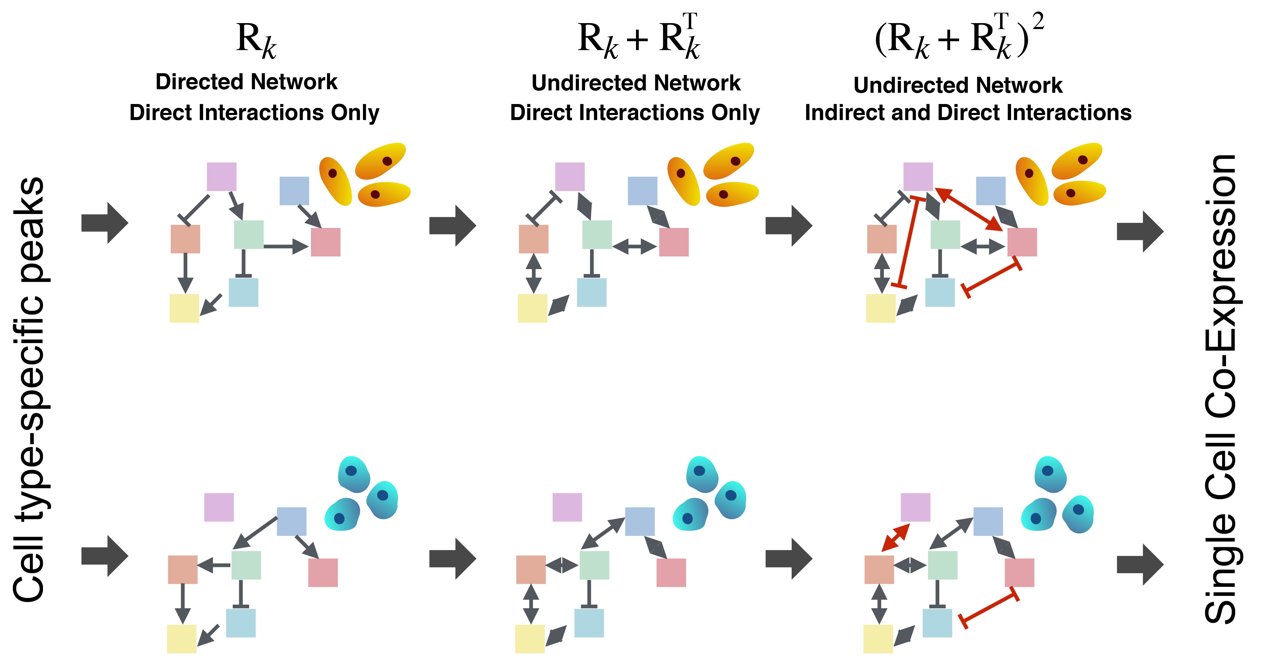
Figure 2: Symphony captures direct and indirect regulation. The impact of regulation ($R_{k}$) is propagated through the network up to path length of two and is reflected in covariance between indirectly connected genes ($\Sigma_{k}$).

1 Introduction

Joint analysis of different types of data that are associated with the same underlying phenomenon is more informative than analysis of individual data types, and increases signal to noise ratio (Xu et al., 2013; Wang et al., 2013; Rey & Roth, 2012). This approach, known as multi-view learning or learning with multiple distinct features, has been successfully used in various settings (Li et al., 2002; Jones & Viola, 2003; Hardoon et al., 2004; Pan et al., 2007).

Here, we apply such a multi-view learning approach to address an important biological problem by integrating two views of gene regulation. Our goal is to infer cell clusters (characterizing cell types) as well as their underlying gene regulatory networks (GRNs), which are directed weighted networks between genes depicting the extent to which a regulatory gene influences the expression of each of its downstream target genes. Understanding differences between regulatory mechanisms across different cell types provides valuable insight in normal development of cell types (Davidson, 2010), and mechanisms disrupted in cancer cells (Pe’er & Hacohen, 2011; Kreeger & Lauffenburger, 2009).

Recent advances in single-cell genomic technologies (Hashimshony et al., 2012; Jaitin et al., 2014; Shalek et al., 2013) which measure gene expression at the resolution of individual cells, present remarkable opportunities to characterize different cell types by clustering cells based on heterogeneity of gene expression (as observed features) (Satija et al., 2015; Macosko et al., 2015). Learning GRNs from gene expression data alone, however, leads to detection of spurious network links based on correlated genes, while integrative learning from multiple data sources has been shown to improve overall joint inference (Zhu et al., 2008; Hecker et al., 2009; Azizi et al., 2014). Therefore, we aim to identify GRNs driving heterogeneous cell types through integrating single-cell expression data with other genomic data types. In particular, epigenetic technologies such as ATAC-seq (Buenrostro et al., 2015a), scan the genome for accessible DNA regions, identifying potential interaction between a gene and regulator proteins translated from other genes. In other words, epigenetic data contains information about direct regulatory links between genes and incorporation of epigenetic data is a promising direction for improved inference of GRNs (Guo et al., 2017; Rotem et al., 2015).

We present a novel integrative model, which we refer to as Symphony, as a Dirichlet process mixture model that jointly learns clusters of cells and GRNs specific to each cluster. Symphony is an extension of the BISCUIT model (Prabhakaran et al., 2016; Azizi et al., 2018) which clusters cells while simultaneously distinguishing biological heterogeneity from technical noise in single-cell gene expression data. This is done through incorporating cell-specific parameters scaling the cluster means and covariances for a multivariate Gaussian mixture model.

We extend the BISCUIT model and replace the hyperparameters with a generative process exclusively driven by the paired epigenetic data, which captures the biological mechanism responsible for observed gene covariances per cell type. Briefly, the epigenetic profiles which denote accessible DNA in the bulk samples are deconvolved into cell-type specific accessible regions (Figure 1). Within these regions, the binding of regulatory proteins translated from genes impacts the expression of nearby genes, such that accessible regions may be mapped to gene-gene interactions. This mapping is based on prior knowledge of recurring DNA sequences (known as motifs) associated with these regulatory proteins which occur in regions of accessible DNA. Most importantly, the covariance in observed gene expression is related to a graph power of the regulatory network, capturing the propagated impact of regulation in the network (indirect regulation)(Figure 2).

This multi-view framework can also be applied to other settings, such as text characterization. For example, to learn the context of queries (vector of words), the bag-of-words simplification may not be sufficient (Biemann, 2005). However, the order of words, which can be represented as a latent directed network can imply the context, and incorporating observations from this network such as the frequency of one word following another (as a second view) can enhance extraction of context and clustering of queries (observed as the first view) (Landauer et al., 1997; Recchia & Jones, 2009).

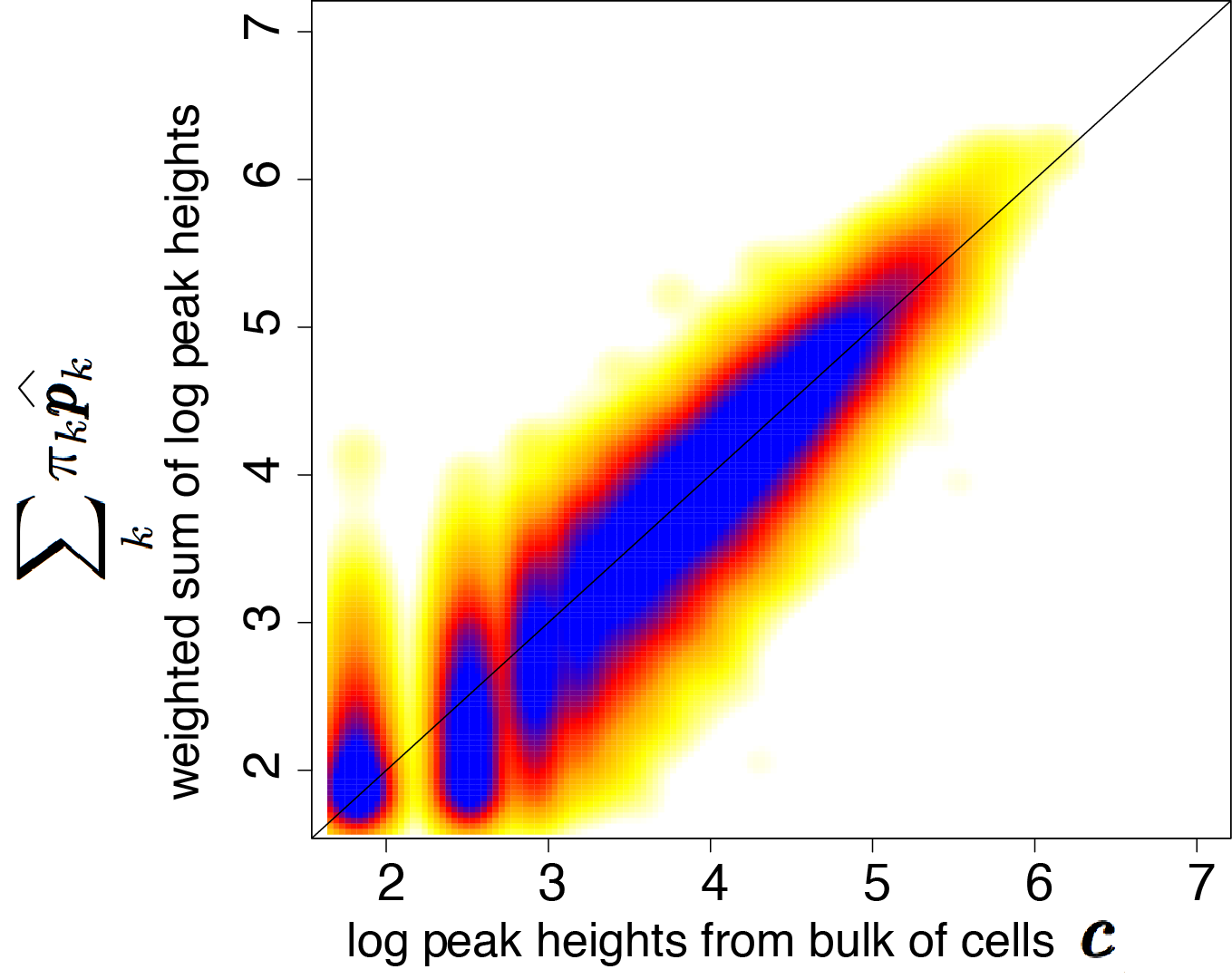
Figure 3: Validation of model assumption. Weighted sum of actual peak heights $\hat{\boldsymbol{p}}_{k}$s measured from sorted clusters of CD34+ hematopoeitic cells using ATAC-seq, with weights proportional to proportions of cell types, compared to measured peak height from ATAC-seq on the bulk of cells $\boldsymbol{c}$; heatmap shows density with yellow (low) to blue (high).

Related technologies and methods. The problem of inferring GRNs specific to cell types involves identifying differences in gene-gene interactions across cell types. However, in most cases the cell types are not well-characterized, hence gene markers are not known to enable sorting of cell types prior to measuring epigenetic data (gene-gene interactions). Therefore, epigenetic data measured on the bulk of cells represents a mixture of cell type-specific epigenetic profiles. One solution is measuring epigenetic profiles at the resolution of single cells. These technologies have only recently emerged (Buenrostro et al., 2015b); we therefore constructed a model to allow integration of bulk ATAC-seq data. Symphony can be easily adapted for inferring GRNs from single-cell ATAC-seq data as well.

Other works have attempted to apply computational deconvolution algorithms intended for bulk expression data, such as those using source separation techniques (Houseman et al., 2016), NMF-based methods (Repsilber et al., 2010) or Bayesian models (Erkkilä et al., 2010), to instead infer cell type-specific epigenetic profiles. Recent methods such as SCENIC (Aibar et al., 2017) infer GRNs from single-cell expression data alone and do not incorporate epigenetic or other types of data.

Contributions. In this paper, we show that a multi-view learning framework would improve the deconvolution of epigenetic data. Furthermore, using an integrative model, we improve the clustering of cells, and hence characterization of cell types. Most importantly, our model presents the advantage of inferring cell type-specific GRNs that give insight into heteroegeneity of underlying mechanisms across cell types. We present a Variational EM inference procedure and show that the integration guarantees model identifiability, while learning from the epigenetic view alone does not. While other works have attempted to integrate bulk multi-omics data (Lake et al., 2017; Brown et al., 2013; Ritchie et al., 2015), there are no methods to our knowledge that infer heterogeneous GRNs through integrating epigenetic and single-cell resolution gene expression data.

Figure 4: Plate model for Symphony. white circles denote latent variables of interest, diamonds are hyperparameters and double diamonds are hyperpriors calculated empirically.

2 Model

The observed data is considered as two views from the biological system (Figure 1):

View 1. Single-cell gene expression data from scRNA-seq technologies (Klein et al., 2015; Macosko et al., 2015) denoted as $X^{d\times n}=[\boldsymbol{x}_{1},\cdots,\boldsymbol{x}_{j},\cdots,\boldsymbol{x}_{n}]$ where each observation $\boldsymbol{x}_{j}\in\mathbb{R}^{d}$ for cell $j\in\{1,\cdots,n\}$ corresponds to $d$ genes (as features). Each entry $x_{ij}$ for $i=[1,\cdots,d]$ contains the expression of gene $i$ in cell $j$ (more precisely, the log of counts of mRNA molecules per gene $i$ from cell $j$ plus a pseudo-count).

View 2. Epigenetic data, for example measured with ATAC-seq technology (Buenrostro et al., 2015a), denoted as $C^{l\times r}=[\boldsymbol{c}_{1},\cdots,\boldsymbol{c}_{t},\cdots,\boldsymbol{c}_{r}]$ where each observation $\boldsymbol{c}_{t}\in\mathbb{R}^{l}$ for $t\in\{1,\cdots,r\}$ corresponds to $l$ genomic regions (as features). Specifically, $\boldsymbol{c}_{t}$ is an experimental replicate measuring accessibility of genomic regions $m=[1,\cdots,l]$.

Prior knowledge. The genomic regions in $C$ can be mapped to genes in $X$ with a pre-defined mapping function $g(i,i^{\prime})=m$ that relates each genomic region $m\in\{1,\cdots,l\}$ to a gene-gene interaction $i^{\prime}\rightarrow i$ for $i,i^{\prime}\in\{1,\cdots,d\}$. We also define $M^{d\times d}$ based on prior knowledge containing binary values $M_{i,i^{\prime}}=1$ if the motif sequence for gene $i^{\prime}$ exists in the genomic region $m$ in the vicinity of gene $i$, meaning a potential interaction can exist from gene $i^{\prime}$ to gene $i$.

2.1 Epigenetic Model (View 2)

The epigenetic data is informative of network structure, i.e. existence of edges between genes (features) and gene expression data contains information on network nodes. We aim to infer this directed weighted network (GRN) for each cluster $k\in\{1,\cdots,K\}$ of cells, denoted by the asymmetric matrix $R_{k}^{d\times d}$ in which entry $R_{k_{i,i^{\prime}}}\neq 0$ if $i^{\prime}\rightarrow i$, meaning gene $i^{\prime}$ directly regulates gene $i$. $R_{k_{i,i^{\prime}}}$ is the regulatory function of gene $i^{\prime}$ on gene $i$ in cluster $k$ such that $R_{k_{i,i^{\prime}}}>0$ or $R_{k_{i,i^{\prime}}}<0$ represent activation or repression of expression respectively, with $|R_{k_{i,i^{\prime}}}|$ being the strength of regulation.

We do not aim to distinguish all layers of the regulatory process (such as protein phosphorylation) and rather interpret GRNs as an approximation for the overall impact of TFs on target genes at the transcriptional level.

We model regulation of gene expression as follows: Genome accessibility in cluster $k$ is represented with latent variable ${\boldsymbol{p}}_{k}=[p_{k}^{1},\cdots,p_{k}^{l}]^{T}\in{\mathbb{R}^{+}}^{l}$ containing $l$ genomic regions (features). This represents log of peak heights plus 1 (to ensure positive domain) in all genomic regions, for each cell type $k$. We set a truncated multivariate Normal prior to capture the structure between genomic regions encompassing co-regulated genes (i.e. genes sharing regulators) with mean $\boldsymbol{\eta}$ and covariance $\Lambda$: $\quad\boldsymbol{p}_{k}\sim trunc\mathcal{N}(\boldsymbol{\eta},\Lambda,\boldsymbol{0},+\infty).\quad$In this paper, we assume a setting where we do not observe $\boldsymbol{p}_{k}$s, and only observe epigenetic data from the bulk of cells which can be represented as a weighted sum of cluster-specific epigenetic profiles where $\pi_{k}$s are weights. Thus, our epigenetic model is:

$$\begin{split}\{\boldsymbol{c}\}_{t}^{(1,\cdots,l)}|{\boldsymbol{p}}_{k},\pi_{k}&\stackrel{{\scriptstyle\text{ind}}}{{\sim}}\mathcal{N}(\sum_{k}\pi_{k}{\boldsymbol{p}}_{k},\zeta I)\end{split}$$ (1)

We validated the above assumption of weighted sum using ATAC-seq data from hematopoeitic progenitor cells from Corces et al. (2016) by computing the weighted sum of measurements from sorted cell types (actual $\boldsymbol{p}_{k}$s denoted with $\hat{\boldsymbol{p}}_{k}$) to measurements from the bulk of cells as $\boldsymbol{c}$ (Figure 3).

We have a $K$-order Dirichlet prior over $\pi_{k}$: $\pi_{k}|\varphi,K\sim\mathit{Dir}(\pi_{k}|\tfrac{\varphi}{K},\cdots,\tfrac{\varphi}{K})$, where $\varphi^{-1}\sim\mathit{Gamma}(1,1)$. Then, in cell type $k$, if a genomic region $m$ in the vicinity of gene $i$ is accessible with log peak height $p_{k}^{m}$, and the motif sequence associated with one or more Transcription Factor (TF) proteins translated from genes $i^{\prime},i^{\prime\prime},...$ exists in the region ($M_{i,i^{\prime}}=M_{i,i^{\prime\prime}}=1$), then the TF(s) can bind to the region and hence regulate the expression of gene $i$. Furthermore, we assume the peak height (strength of TF binding to genome) is informative of $i^{\prime}\rightarrow i$ edge weight $|R_{k}|$ (strength of regulation). Thus, we model $R_{k}$ as follows:

$$\begin{split}R_{k}^{i,i^{\prime}}&\sim\mathcal{N}(S^{i,i^{\prime}}M^{i,i^{\prime}}\boldsymbol{p}_{k}^{g(i,i^{\prime})},\lambda)\end{split}$$ (2)

The function $g(\cdot)$ maps gene pair $i,i^{\prime}$ to genomic region $l$. $S$ denotes a sign indicator variable representing repression or activation function. We set $S$ according to the sign of the empirical covariance: $S^{i,i^{\prime}}=sign(\Sigma^{\prime\prime^{i,i^{\prime}}})$.

2.2 Single-cell Gene Expression Model (View 1)

We use the above epigenetic model to drive gene expression data based on the following key ideas: First, if a direct regulatory link exists from a TF associated with gene $i^{\prime}$ to a target gene $i$ ($i^{\prime}\rightarrow i$), we assume there is strong covariance between their expressions. Second, due to van der Corput’s inequality (Montgomery, 2001), covariances can partly reflect the propagated impact of indirect regulation in cases where genes are not directly connected but exist on the same path in the network (Figure 2). For example if $i^{\prime\prime}\rightarrow i^{\prime}$ and $i^{\prime}\rightarrow i$, we might also observe covariance between $i,i^{\prime\prime}$ even though they are not directly connected in the network (e.g. $R_{k}^{i,i^{\prime\prime}}=0,\Sigma_{k}^{i,i^{\prime\prime}}\neq 0$). Here, we consider indirect effects with path length up to two using the square of the indirected network $(R_{k}+R_{k}^{T})^{2}$ (Walker, 1992) such that:

$$\begin{split}\Sigma_{k}^{-1}|R_{k}&\sim\mathit{Wish}({(R_{k}+R_{k}^{T})}^{-2},\gamma)\\ \end{split}$$ (3)

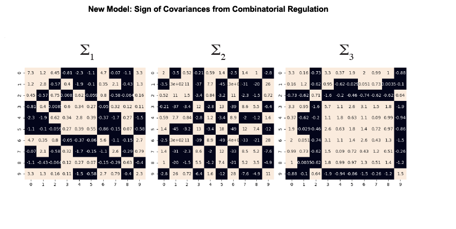
Figure 12: Examples of synthetic $\Sigma_{k}$ simulated from the same $S$ matrix for clusters $k=1,2,3$, showing variability in sign of $\Sigma_{k}$ that can capture the impact of combinatorial regulations.

${(R_{k}+R_{k}^{T})}^{2}$ is positive semi-definite according to Lemma 3 in the following section making the above modeling assumption feasible. Additionally, this model can capture combinatorial regulation in the inferred covariances. In particular, a gene pair $i,i^{\prime}$ will always have the same directionality of regulation (i.e. activation or repression relationship), but $\Sigma_{k}^{i,i^{\prime}}$ can be positive in one cluster and negative in another cluster depending on the relative regulatory strength of activators and regulators in its path. An example of this variability in sign is shown in Supplmentary Figure 12.

Gene expression data for each cell $j$ denoted as $\boldsymbol{x}_{j}$ is then modeled similar to the multivariate Gaussian mixture model in BISCUIT:

$$\begin{split}\{\boldsymbol{x}\}_{j}^{(1,\cdots,d)}|z_{j}=k\stackrel{{\scriptstyle\text{ind}}}{{\sim}}&\mathcal{N}(\alpha_{j}\boldsymbol{\mu}_{k},\beta_{j}\Sigma_{k})\\ \boldsymbol{\mu}_{k}\sim\mathcal{N}(\boldsymbol{\mu}^{\prime},\Sigma^{\prime}),&\quad\boldsymbol{\mu}^{\prime}\sim\mathcal{N}(\boldsymbol{\mu}^{\prime\prime},\Sigma^{\prime\prime})\\ \Sigma^{\prime-1}\sim\mathit{Wish}(d,\frac{1}{d\Sigma^{\prime\prime}}),&\quad z_{j}|\pi_{k}\stackrel{{\scriptstyle\mathrm{iid}}}{{\sim}}\mathit{Mult}(z_{j}|\pi_{k})\\ \alpha_{j}\sim log\mathcal{N}(\nu,\delta^{2}),&\quad\beta_{j}\sim log\mathcal{N}(\omega,\theta)\end{split}$$ (4)

where $z_{j}$ denotes assignment of cell $j$ to cluster $k\in\{1,\cdots,K\}$. With integrating two data modalities (gene expression and epigenetic data), we improve inference of clusters (cell types). The scaling parameters $\alpha_{j},\beta_{j}$ specific to cell $j$ are used to normalize the data $\boldsymbol{x}_{j}$ in downstream analysis by transforming to $\boldsymbol{y}_{j}\sim\mathcal{N}(\boldsymbol{\mu}_{k},\Sigma_{k})$ according to the cluster it is assigned to $z_{j}=k$, similar to Prabhakaran et al. (2016). The plate model for Symphony is summarized in Figure 4.

3 Theory

We show theoretical advantages of integration of the two data types using Symphony as follows: We define $f(\boldsymbol{x}):=\mathcal{N}(\alpha\boldsymbol{\mu}_{k},\beta\Sigma_{k})\in\mathbb{R}^{d}$ as the multivariate Gaussian density of $\boldsymbol{x}$ and $f(\boldsymbol{c}):=\mathcal{N}(\sum_{k}\pi_{k}{\boldsymbol{p}}_{k},\zeta I)\in\mathbb{R}^{l}$ as the multivariate Gaussian density of $\boldsymbol{c}$. First, we emphasize that the epigenetic model alone $f(\boldsymbol{c}|\boldsymbol{p}_{k},\pi_{k},\zeta)$ is not identifiable and therefore precise inference of deconvolved epigenetic profiles ($\boldsymbol{p}_{k}$s) is not possible:

Lemma 1

The epigenetic model $f(\boldsymbol{c}|\boldsymbol{p}_{k},\pi_{k})$ is non-identifiable (Proof in Supplementary section B)

This motivated us to build an integrative model. Identifiability of the single-cell expression model $f(\boldsymbol{x}|\boldsymbol{\mu}_{k},\Sigma_{k},\boldsymbol{\alpha},\boldsymbol{\beta},\boldsymbol{z})$ has been shown under certain enforced constraints on both $\boldsymbol{\alpha,\beta}$:

Lemma 2

(Prabhakaran et al., 2016) Defining $\Phi=\{\forall j,k:(\alpha_{j},\boldsymbol{\mu}_{k},\beta_{j},\Sigma_{k})\}\cup\{\boldsymbol{\pi}\}$$\Phi=\Phi^{\star}$ if the following conditions hold: $\forall j:\boldsymbol{\mu}_{k}\geq\boldsymbol{\mu}^{\prime}+diag(\Sigma^{\prime})(\alpha_{j}-\nu)/\delta$ and $\forall j:\beta_{j}\geq\frac{\theta}{\omega+1}$

While the above conditions guarantee identifiability, they are not inferred from data or biologically motivated and hence interpretation of parameters may not provide the best characterization of cell types. Here, we show that in the integrative model, the constraints for $\beta_{j}$s are no longer required and identifiability of the expression model $f(\boldsymbol{x}|\boldsymbol{\mu}_{k},\Sigma_{k},\boldsymbol{\alpha},\boldsymbol{\beta},\boldsymbol{z},\boldsymbol{p}_{k},R_{k})$ is guaranteed through the extension of the model that captures regulation, from which we observe additional epigenetic data $\boldsymbol{c}$. Hence the full model $f(X,C|\{\boldsymbol{\mu}_{k},\Sigma_{k},\boldsymbol{\alpha},\boldsymbol{\beta},\boldsymbol{z},\boldsymbol{p}_{k},R_{k},\pi_{k},\zeta\})$ is identifiable. We will use the following lemma to show $(R_{k}+R_{k}^{T})^{2}$ is positive semi-definite.

Lemma 3

Square of a symmetric matrix $H$ gives a symmetric positive semi-definite matrix $L$ (Proof in Supplementary section B).

Since single-cell expression data $X$ usually contains expression of genes that do not have observations in their mapped genomic regions in $\boldsymbol{c}$ such that $d>l$, we first define a reduced version of the model where all genes in $\boldsymbol{x}$ do have mapped genomic regions: $f(X^{0},C)$ where $X^{0}$ is a ${l\times n}$ subset of $X$. Then, $f(\boldsymbol{x}^{0}_{l\times 1})=\mathcal{N}(\alpha\boldsymbol{\mu}_{k}^{0},\beta\Sigma_{k}^{0})$ with $\boldsymbol{\mu}_{k}^{0},\Sigma_{k}^{0}$ being subsets of $\boldsymbol{\mu}$ and $\Sigma$. We next show the identifiability of the reduced model. Then, we use this result to extend the identifiability to the full model given $\boldsymbol{\beta}$ which is the parameter scaling $\Sigma_{k}$. Finally, we show the identifiability of the full model.

Lemma 4

In the reduced model: $f(X^{0},C|\boldsymbol{\beta},\boldsymbol{\mu}_{k}^{0},\Sigma_{k}^{0},\boldsymbol{\alpha},\boldsymbol{z},\boldsymbol{p}_{k},R_{k}^{0},\pi_{k},\zeta)$, $\beta$s are identifiable under the conditions of: $\forall j:\boldsymbol{\mu}_{k}\geq\boldsymbol{\mu}^{\prime}+diag(\Sigma^{\prime})(\alpha_{j}-\nu)/\delta$ without the need for condition on $\beta$s (Proof in Supplementary section B).

Lemma 5

For a given $\boldsymbol{\beta}=\beta^{*}$, identifiability of: $f(X,C|\boldsymbol{\mu}_{k},\Sigma_{k},\boldsymbol{\alpha},\boldsymbol{\beta}=\boldsymbol{\beta}^{*},\boldsymbol{z},\boldsymbol{p}_{k},R_{k},\pi_{k},\zeta)$ is guaranteed if $\forall j:\boldsymbol{\mu}_{k}\geq\boldsymbol{\mu}^{\prime}+diag(\Sigma^{\prime})(\alpha_{j}-\nu)/\delta$ (Proof in Supplementary section B).

Theorem 6

The full model $f(X,C|\{\boldsymbol{\mu}_{k},\Sigma_{k},\boldsymbol{\alpha},\boldsymbol{\beta},\boldsymbol{z},\boldsymbol{p}_{k},R_{k},\pi_{k},\zeta\}))$ is identifiable if $\ \forall j:\boldsymbol{\mu}_{k}\geq\boldsymbol{\mu}^{\prime}+diag(\Sigma^{\prime})(\alpha_{j}-\nu)/\delta$ (Proof in Supplementary section B).

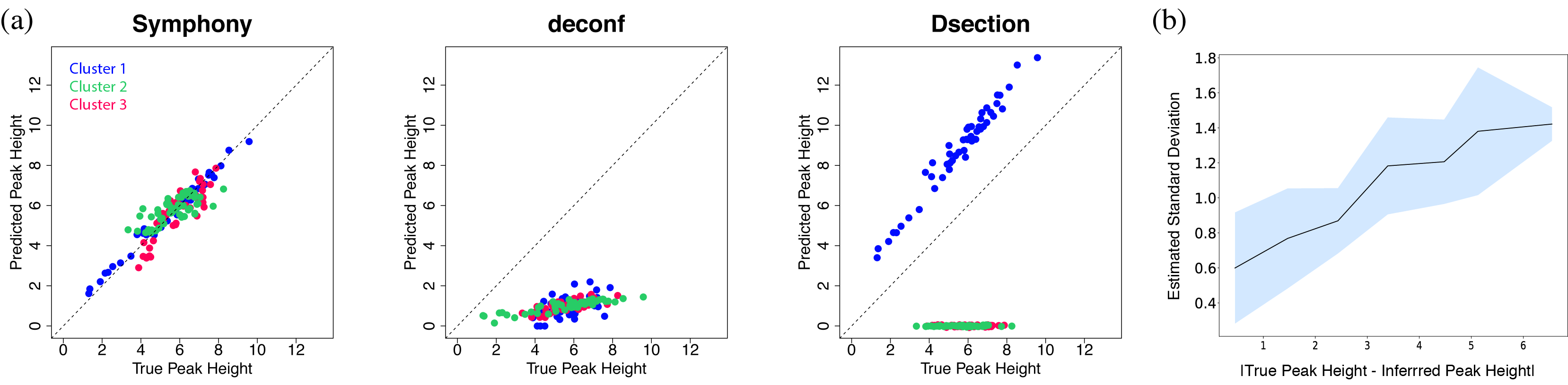
Figure 5: Performance in deconvolving epigenetic data. (a) Estimated peak heights $\boldsymbol{p}_{k}$ using Symphony for $K=3$ synthetic clusters versus true peak heights, compared to two other deconvolution methods: deconf (Repsilber et al., 2010) and Dsection (Erkkilä et al., 2010); each dot represents a genomic region. (b) Moving average of estimated standard deviation for $\boldsymbol{p}_{k}$s using Symphony vs. estimate residual; shaded area shows 1 standard deviation in each window of length 1.

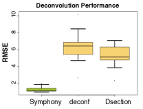
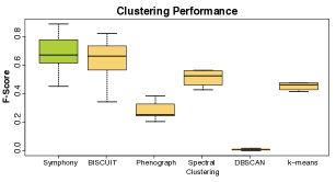
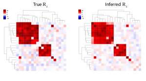
Figure 6: Left: Root-mean-square error (RMSE) in inferring $\boldsymbol{p}_{k}$s across $10$ experiments compared to other deconvolution methods used for genomic data. Middle: Performance in clustering cells across $10$ experiments compared to other clustering methods commonly used for single-cell gene expression data. Right: Heatmap depicting true versus inferred $R_{k}$ in synthetic data showing Symphony’s superior capabilities in recovering underlying $R_{k}$.

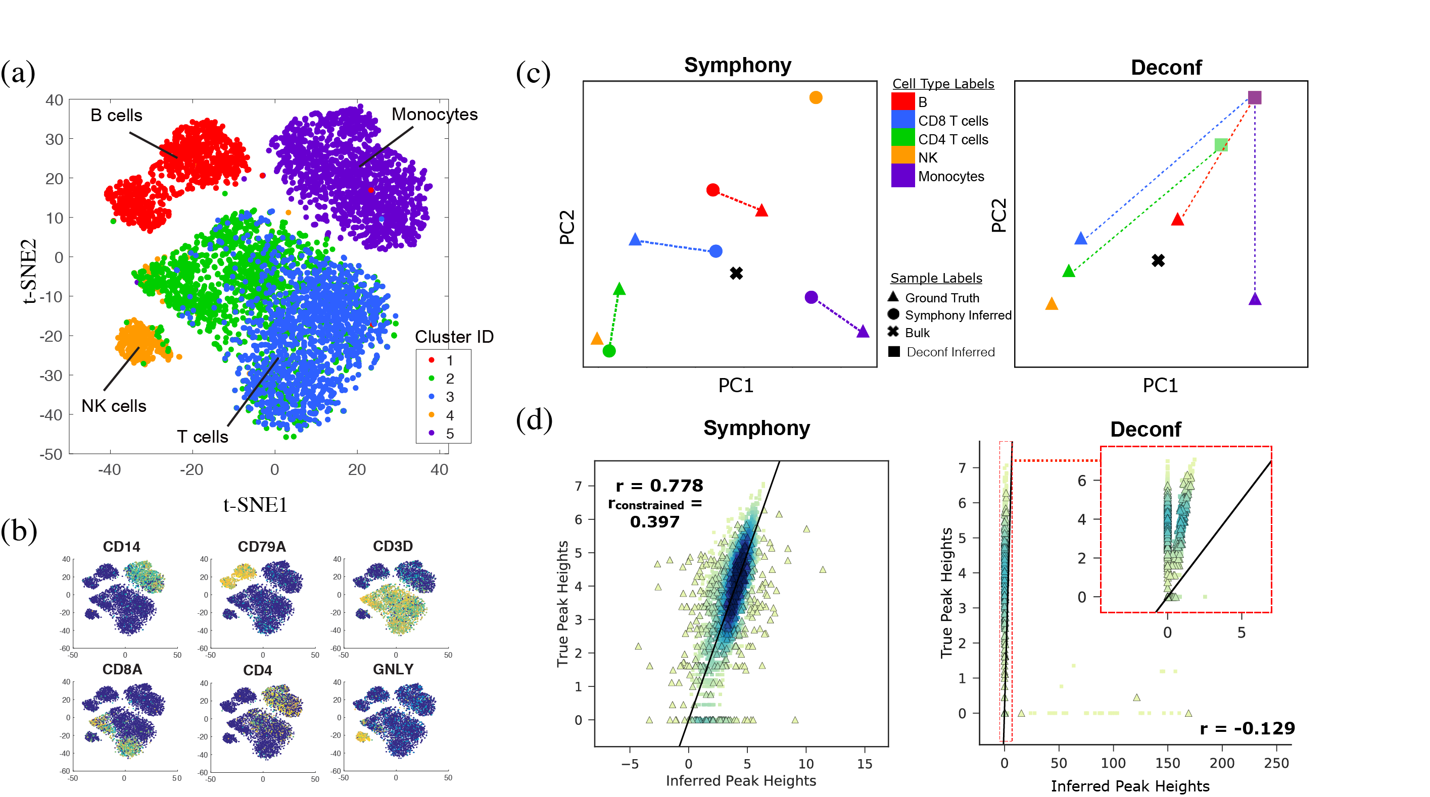
Figure 7: Performance on genomic data from PBMCs. (a) t-SNE map of $6825$ single-cell gene expression data from 5 cell types after normalization, cells colored by clusters (b) expression of cell-type markers (c) PCA on expression-constrained peaks and those which show at least some accessibility in all cell types (to show effective peak magnitude estimation) showing global performance of Symphony in deconvolving epigenetic data; shown with projection of inferred peak heights on principal components of ground truth peak heights (from ATAC-seq on sorted cell types in Corces et al. (2016)) (left) compared to deconvolution using Deconf (right) which fails to deconvolve the majority of peaks shown with overlapping squares (d) Scatterplot of inferred peak heights for all clusters vs ground truth peak height using Symphony (left) compared to Deconf (right); peaks are colored by density; $r$ values show Pearson correlation; peaks constrained by expression data and bulk epigenetic data are triangular points with black outline; NK cells were not included in this plot due to the small cell proportion ($<$ 5%), making deconvolution impossible.

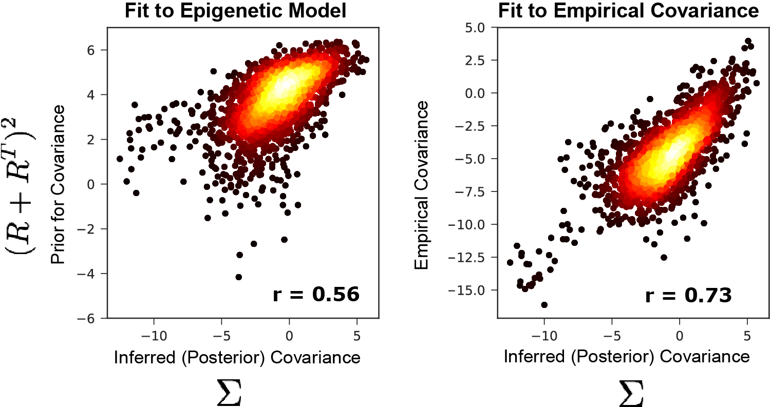
Figure 8: Symphony model fit. Left: Inferred covariance vs its prior capturing direct and indirect regulation $(R+R^{T})^{2}$; Right: Empirical gene covariance compared to inferred covariance across all cell types. All axes are log-transformed.

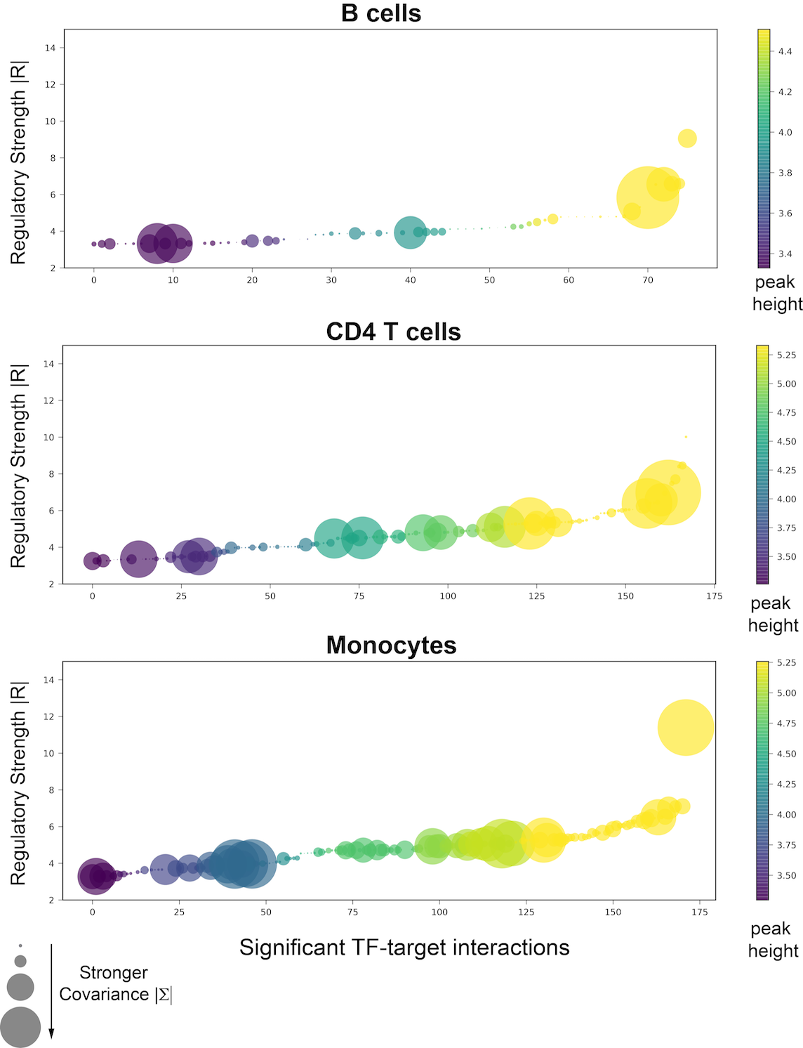
Figure 9: GRN Interpretation. Inferred regulations sorted by strength ($|R|$) show association with either peak heights or TF-target covariance or both; circle sizes are proportional to covariance strength ($|\Sigma|$) and they are colored by inferred peak height per cell type. Covariances are z-normalized for scale.

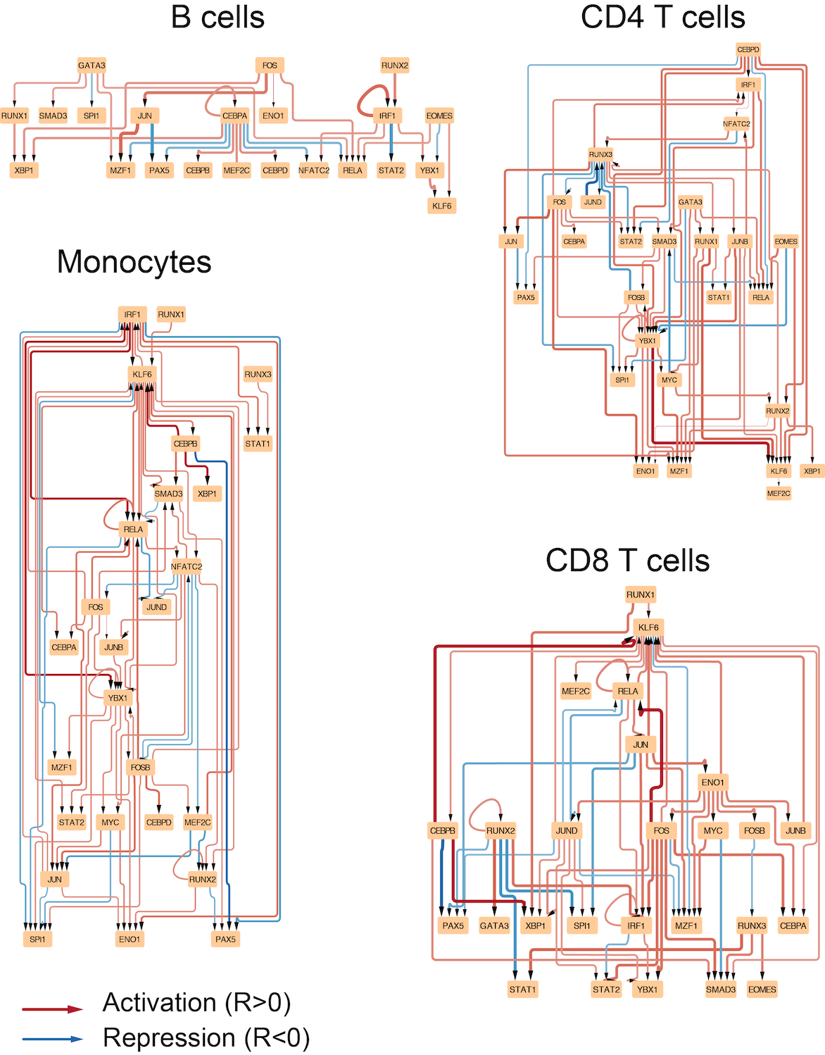
Figure 10: Subnetworks of cell type-specific GRNs between TFs with strongest regulations ($|R_{k}|>4.5$); global structures show differences in connectivity of TFs across clusters (cell types); red and blue edges indicate activation and repression; edge widths are proportional to strength of regulation ($|R|$).

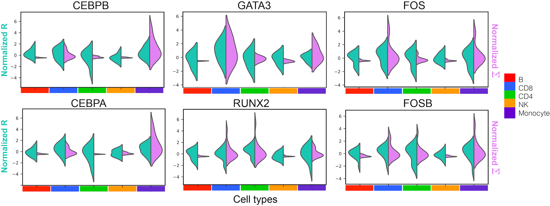
Figure 11: Identification of cell type-specific regulators. Violinplots of inferred cell type-specific regulatory function $R$ (green) for TFs that show variability across cell types, compared to inferred covariance $\Sigma$ (pink) between example TFs (regulators) and all of their target genes; positive and negative signs in $R$ denote activation and repression of expression, respectively; values have been z-score normalized to display both variables on the same y-axis.

4 Inference

We applied the co-ordinate ascent mean field variational inference (CAVI) (Blei et al., 2017; Ghahramani & Beal, 2001) which assigns independent factors to the latent variables. The blueprint for corresponding CAVI updates are below and full derivations are presented in Supplementary section C.

Variational E-step

a. $q^{*}(z_{j})=\prod_{k}r_{jk}^{z_{jk}}$ where

$$\begin{split}r_{jk}=\mathbb{E}_{\boldsymbol{z}}{z_{jk}}\propto&\widetilde{|\beta_{j}\Sigma_{k}|^{-1}}\exp(-S_{2})\widetilde{\pi_{k}},\ \sum_{k}r_{nk}=1\\ S_{2}=&\tfrac{1}{2}\Big{(}\textit{tr}(\Sigma_{k}^{-1}\beta_{j}^{-1}\Sigma^{\prime\prime-1})+\\ &(\boldsymbol{\mu}^{\prime\prime}-\alpha_{j}\boldsymbol{\mu}_{k})^{T}(\beta_{j}\Sigma_{k})^{-1}(\boldsymbol{\mu}^{\prime\prime}-\alpha_{j}\boldsymbol{\mu}_{k})\Big{)}\\ \widetilde{|\beta_{j}\Sigma_{k}|^{-1}}:=&\frac{1}{2}(-d\mathbb{E}_{\beta_{j}}\ln\beta_{j}+\\ &d\ln(2)+\ln|R^{*}_{k}|+\sum_{i=1}^{d}\psi\Big{(}\frac{\gamma+1-i}{2}\Big{)})\\ \end{split}$$ (5)

where $\ln\widetilde{\pi_{k}}:=\psi(\varphi_{0})-\psi(\sum_{k}\varphi_{k})$ and $\psi$ is the digamma function and $R^{*}_{k}=(R_{k}+R_{k}^{T})^{2}$.

Variational M-step

$$\begin{split}\textbf{b. }q^{*}(\pi_{k})=&\pi_{k}\sim\text{Stick-breaking Beta}(1,\varphi)\\ \textbf{c. }q^{*}(\boldsymbol{\mu}_{k})=&\exp\Big{(}-\tfrac{1}{2}\sum_{j}r_{jk}\Big{(}\textit{tr}(\Sigma_{k}^{-1}(\tfrac{\beta_{j}}{\alpha_{j}^{2}})^{-1}\Sigma^{\prime\prime-1})\\ &+(\bar{\boldsymbol{\mu_{k}}}-\frac{x_{j}}{\alpha_{j}})^{T}{(\frac{\beta_{j}}{\alpha_{j}^{2}}\Sigma_{k})}^{-1}(\bar{\boldsymbol{\mu_{k}}}-\frac{x_{j}}{\alpha_{j}})\\ &+(\boldsymbol{\mu}_{k}-\boldsymbol{\mu}^{\prime})^{T}\Sigma^{\prime-1}(\boldsymbol{\mu}_{k}-\boldsymbol{\mu}^{\prime})\Big{)}+c\Big{)}\\ \end{split}$$ (6)

$$\begin{split}\textbf{d. }q^{*}(\Sigma_{k}^{-1})=&\exp\Big{(}-\tfrac{1}{2}\sum_{j}r_{jk}\Big{(}\ln\beta_{j}^{d}+\ln|\Sigma_{k}|\\ &+\tfrac{1}{\beta_{j}}\Big{(}\textit{tr}(\Sigma_{k}^{-1}\Sigma^{\prime\prime-1})\\ &+(\boldsymbol{\mu}^{\prime\prime}-\alpha_{j}\boldsymbol{\mu}_{k})^{T}(\Sigma_{k})^{-1}(\boldsymbol{\mu}^{\prime\prime}-\alpha_{j}\boldsymbol{\mu}_{k})\Big{)}\Big{)}\\ &+\ln|\Sigma_{k}^{-1}|^{\frac{\lambda-d-1}{2}}+\{-\frac{tr(R^{*-1}_{k}\Sigma_{k}^{-1})}{2}\}\\ &-\ln(2^{\lambda d/2}|R^{*-1}_{k}|^{-\lambda/2}\Gamma_{d}(\lambda/2))+c\Big{)}\\ \textbf{e.}q^{*}(\alpha_{j})=&\exp\Big{(}-\sum_{k}r_{jk}S_{2}\\ +\frac{1}{\sqrt{2\delta^{2}\pi}}&\exp\Big{(}-\frac{(\ln\alpha_{j}-\nu)\mathbb{I}_{1\times 1}(\ln\alpha_{j}-\nu)}{2\delta^{2}}\Big{)}+c\Big{)}\\ \textbf{f. }q^{*}(\beta_{j})=&\exp\Big{(}-\sum_{k}r_{jk}S_{2}\\ +\frac{1}{\sqrt{2\theta^{2}\pi}}&\exp\Big{(}-\frac{(\ln\beta_{j}-\omega)\mathbb{I}_{1\times 1}(\ln\beta_{j}-\omega)}{2\theta^{2}}\Big{)}+c\Big{)}\\ \textbf{g. }q^{*}(\boldsymbol{\mu}^{\prime})\sim&\mathcal{N}(\boldsymbol{\mu}_{\mu^{\prime}},\Sigma_{\mu^{\prime}})\\ \end{split}$$ (7)

$$\begin{split}\textbf{h. }q^{*}(\Sigma^{-1\prime})&\sim\mathcal{W}(V_{\Sigma^{\prime-1}},d_{\Sigma^{\prime-1}})\\ \textbf{i. }q^{*}(R_{k})=&\exp\Big{(}\{-\frac{tr(R^{*-1}_{k}\Sigma_{k}^{-1})}{2}\}\\ -\ln(2^{\lambda d/2}&|R^{*-1}_{k}|^{-\lambda/2}\Gamma_{d}(\lambda/2))\\ -\tfrac{1}{2\delta^{2}}\sum_{i}\sum_{i^{\prime}}&\Big{(}(R_{k}^{i,i^{\prime}}-S^{i,i^{\prime}}M^{i,i^{\prime}}\boldsymbol{p}_{k}^{g(i,i^{\prime})})\mathbb{I}_{1\times 1}(R_{k}^{i,i^{\prime}}-\\ &S^{i,i^{\prime}}M^{i,i^{\prime}}\boldsymbol{p}_{k}^{g(i,i^{\prime})})\Big{)}+c\Big{)}\\ \textbf{j.}q^{*}(\boldsymbol{p}_{k})=\exp&\Big{(}(\bar{c}_{t}-\sum_{k}(\pi_{k}\boldsymbol{p}_{k}))^{T}(\zeta\mathbb{I})^{-1}(\bar{c}_{t}-\sum_{k}(\pi_{k}\boldsymbol{p}_{k}))]\\ +\ln&\Big{(}\tfrac{1}{\sqrt{2\pi}\Lambda}\exp(-\tfrac{1}{2}(\tfrac{\boldsymbol{p}_{k}-\eta}{\Lambda})^{2}))\Big{)}\\ -\tfrac{1}{2\delta^{2}}&\sum_{i}\sum_{i^{\prime}}\Big{(}(R_{k}^{i,i^{\prime}}-S^{i,i^{\prime}}M^{i,i^{\prime}}\boldsymbol{p}_{k}^{g(i,i^{\prime})})\mathbb{I}_{1\times 1}\\ &(R_{k}^{i,i^{\prime}}-S^{i,i^{\prime}}M^{i,i^{\prime}}\boldsymbol{p}_{k}^{g(i,i^{\prime})})\Big{)}+c\Big{)}\end{split}$$ (8)

where $c$ is the integration constant (details are included in Supplementary section C). Since the E-step takes $\approx\mathrm{O}(d^{3})$ due to three matrix inversions, we substitute this with $z_{\small{MAP}}(\boldsymbol{x})=\arg\max_{z}p(\boldsymbol{x}|\boldsymbol{z})p(\boldsymbol{z}|\boldsymbol{\pi})$ which takes $\approx\mathrm{O}(d^{2})$ when $\Sigma_{k}^{-1}$s and $\Sigma^{\prime\prime}$ are apriori Cholesky decomposed.

Given the complexity of the model (refer to Supplementary section C), we implemented Symphony using the probabilistic programming language Stan (Carpenter et al., 2016). Furthermore, for a scalable implementation applicable to real genomic data containing thousands of cells, we used the probabilistic programming language, Edward (Tran et al., 2016, 2017) for variational EM (details and approximations presented in Supplementary section E).

5 Results

5.1 Synthetic Data

We first evaluated the performance in deconvolving epigenetic data, clustering cells, and inferring GRNs using data simulated from the Symphony model. We simulated data for $n=100$ cells in $K=3$ clusters with $d$ ranging from $5$ to $20$ genes and $l=50$ using the Symphony model.

Inference of $\boldsymbol{p}_{k},R_{k}$. Figure 5(a) shows scatterplots of deconvolved peak heights ($\boldsymbol{p}_{k}$) compared to actual data. We compared the performance of Symphony to two other deconvolution methods: deconf (Repsilber et al., 2010) which uses NMF, and Dsection (Erkkilä et al., 2010) which is based on a Bayesian model. While Dsection captures only the largest cluster, deconf underestimates the cluster-specific peak heights. The behavior of Dsection was reproducible across simulations, and is likely due to the lack of identifiability in the model for epigenetic data alone, as discussed above.

Figure 6 summarizes the error in estimating $\boldsymbol{p}_{k}$s across $10$ synthetic datasets with the same size as above. This shows the value of incorporating expression data (view 1) in deconvolution of epigenetic data (view 2). Figure 6 also shows a heatmap of inferred $R_{k}$ in one of the synthetic experiments as an example, compared to the actual $R_{k}$, confirming the ability of Symphony in inferring GRNs.

Clustering performance. We then show the performance in clustering with integrating both views as compared to only using gene expression data (view 1) by computing F-scores across $10$ experiments with the same size as above. We compared the performance to BISCUIT (Prabhakaran et al., 2016), as well as other methods commonly used for clustering cells in single-cell gene expression data including DBscan (Satija et al., 2015), Phenograph (Levine et al., 2015), Spectral clustering (Ng et al., 2002) and k-means (with $K=3$) (Figure 6). These results show improvement over BISCUIT due the epigenetic extension of the model and significant improvement over other methods. DBscan was unable to cluster the majority of cells, likely due to the small dimensionality of the feature space used in simulations. This shows the value of incorporating epigenetic data (view 2) in improving clustering performance, as compared to using expression data (view 1) alone. This has further value in biological interpretation of clusters as cell types that have both similar expression and similar underlying mechanisms driving expression.

5.2 Genomic Data

We also evaluated the performance of Symphony on real genomic data. We used previously published single-cell expression data for peripheral blood mononuclear cells (PBMCs) from Zheng et al. (2017) combined with ATAC-seq data for PBMCs from Corces et al. (2016). For single-cell expression data, we chose a subset of PBMCs from (Zheng et al., 2017) as $X$ containing $n=6825$ cells which express known gene markers for either monocytes, B cells or T cells and NK cells. We chose to focus on $d=28$ transcription factors which showed high standard deviation in expression data and are known to be lineage-defining factors.

For epigenetic data matching the above cell types, we generated $r=1$ mixture of epigenetic measurements with $l=1053$ peaks from real ATAC-seq data collected from the above sorted cell types in Corces et al. (2016), with weights $\pi_{k}$ proportional to frequency of cell types in blood, and used this as observed epigenetic data $C$. We fixed the clustering in this experiment using Phenograph-derived assignments which we mapped onto nearest cell types to match with epigenetic data (Levine et al., 2015).

We determined non-zero entries in $M$ from ATAC-seq using the FIMO algorithm (Grant et al., 2011), which scans the sequence under the ATAC-seq peak for the occurrence of a motif. We associated a peak with the target gene closest in genomic distance to the peak in these experiments. This assignment is independent of the model structure and can be manually defined by the user.

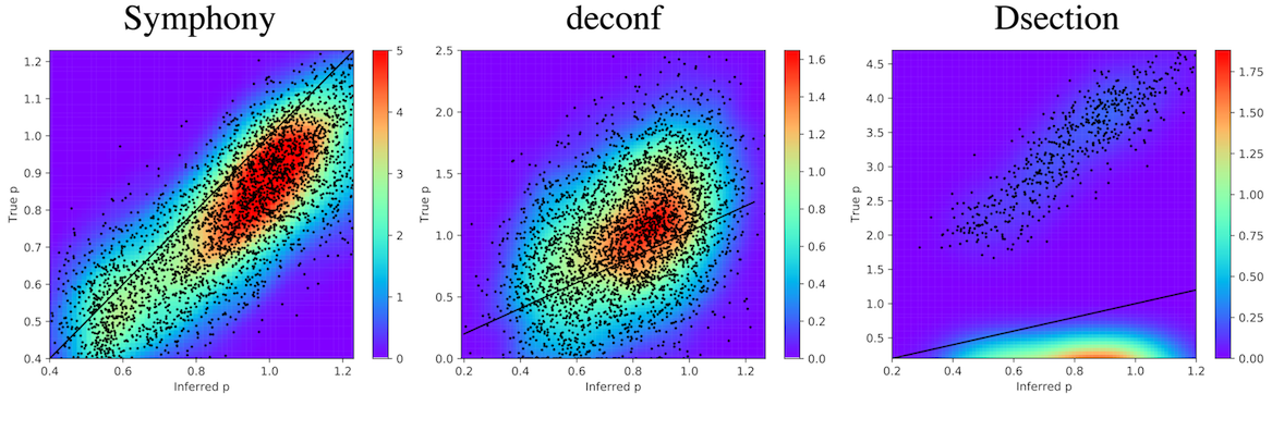
Figure 14: Performance in deconvolving epigenetic data with Edward implementation. Estimated peak heights $\boldsymbol{p}_{k}$ using Symphony for $n=4000$ simulated cells in $K=3$ clusters with $d=100$ genes and $l=550$ versus true peak heights, compared to two other deconvolution methods: deconf (Repsilber et al., 2010) and Dsection (Erkkilä et al., 2010); each dot represents a genomic region; heatmap shows density.

In the following tests, we used a scalable implementation with Edward (Tran et al., 2016) detailed in Supplementary section E. Figure 14 shows the performance of this implementation on a larger number of cells and genes.

Cell type characterization. In this test, we pre-imputed and normalized data, and fix BISCUIT-derived normalization parameters ($\alpha,\beta$). Specifically, we normalized and imputed $\boldsymbol{x}_{j}$ for each cell $j$ by transforming it to $\boldsymbol{y}_{j}$ with $\boldsymbol{y}_{j}=A\boldsymbol{x}_{j}+b$, and setting $A=I/\beta_{j}$ and $b=(I-\alpha_{j}A)\boldsymbol{\mu}_{k}$ with BISCUIT -inferred parameters. This transformation corrects for cell-specific technical effects captured by $\alpha_{j}.\beta_{j}$, as $\boldsymbol{y}_{j}\sim\mathcal{N}(\boldsymbol{\mu}_{k},\Sigma_{k})$ while $\boldsymbol{x}_{j}\sim\mathcal{N}(\alpha_{j}\boldsymbol{\mu}_{k},\beta_{j}\Sigma_{k})$ (Figure 4) (Prabhakaran et al., 2016). Figure 7 (a) shows t-SNE projections (Maaten & Hinton, 2008) of $\boldsymbol{y}_{j}$s after normalizing expression data based on inferred parameters $\boldsymbol{\mu}_{k},\Sigma_{k},\boldsymbol{\alpha},\boldsymbol{\beta}$ where cells are colored by cluster assignments $z_{j}$s for $K=5$ distinct cell populations. Figure 7 (b) shows normalized expression of known marker genes used to characterize the clusters as monocyte, B, T and NK cell types.

Deconvolving epigenetic data. Figure 7 (c,d) show inferred peak heights $\boldsymbol{p}_{k}$ for all clusters using Symphony compared to ground truth cell type specific peak heights (measured with ATAC-seq from sorted cell types). Supplementary Figure 13 shows an example genomic region with differential peaks for three of these cell types showing distinct epigenetic profiles. Projection of peak heights to principal components of ground truth peaks (excluding peaks un-constrained by expression data and peaks which show 0 accessibility in some cell types, to show performance at deciphering magnitudes) shows superior performance in deconvolving all subsets of cells except for the smallest population (NK cells, $<5$% of cells). The small error between estimated $\boldsymbol{p}_{k}$s and ground truth cell type-specific peak heights confirms that our model is a good fit for the biological mechanism of regulation. We also evaluated the deconvolution of epigenetic data using deconf (Figure 7 (c)) which shows under-estimation or inaccurate estimation of peak heights. We could not test Dsection as the number of clusters exceeds the number of replicates.

Inferring GRNs. The main advantage of Symphony is the inference of GRNs. Figure 8 shows Symphony can successfully learn cell type-specific covariances comparable to empirical covariances. The gene-gene covariance matrix is then explained by direct regulation as well as the propagated impact of regulation through $(R+R^{T})^{2}$, which we previously validated is capable of capturing epigenetic information through the accuracy of its prior $p$. Furthermore, Figure 9 reveals that inferred regulatory functions are explained by either TF binding strength (peak height) or TF-gene covariance or both.

Figure 10 shows the inferred GRNs between TFs with strongest inferred links ($|R_{k}|>4.5$) in each cluster. The differences in the structure of the networks suggests different mechanisms driving cell type-specific expression.

We observe numerous regulatory interactions that are variable across clusters. Figure 11 shows examples of TF-gene interactions ($R$) that are also supported by known literature. It can be seen that regulatory functions are partially supported by gene-gene covariances ($\Sigma$). We observe $CEBPA,CEBPB$ differentially regulating target genes in monocytes (cluster 5). A recent study (Jaitin et al., 2016) has shown that knock-outs of $CEBPB$ block monocyte differentiation.

We observe regulatory edges in the GRN for T cells between Transcription Factors (TFs) $GATA3,RUNX2$ and their target genes, with minimal interaction in B cells and NK cells (Figure 11), and indeed these TFs are known to be associated with activation of cytotoxic T cells (Pearce et al., 2003) and CD8 T cell development (Woolf et al., 2003). We also observe cases such as $FOS,FOSB$ with different regulatory functions despite belonging to the same TF family, showing an example of how expression-derived information can further distinguish genetic interactions which cannot be immediately deciphered from epigenetic data.

6 Conclusion

We present a hierarchical Bayesian mixture model named Symphony that infers clusters of cells representative of cell types and gene regulatory networks (GRNs) specific to cell types. This is done by modeling the regulatory mechanism driving gene expression in each cell type, and assuming two observations as two views from the system: epigenetic measurements, which are informative of network edges and single-cell gene expression data, informative of network node activity. To the best of our knowledge, this is the first computational method that integrates single-cell expression data with epigenetic data. We provide theoretical justifications for the model and an EM-VI procedure. Symphony shows great performance in clustering cells, deconvolving epigenetic profiles and inferring GRNs in both synthetic and real data from peripheral blood cells and shows superiority to other methods that only address one of these problems. Further, Symphony was able to deconvolve epigenetic data when only one replicate was available through integration of expression data, a potentially common task which would be challenging for any source separation technique. Future iterations of the experiments will allow a Symphony -derived clustering of PBMCs to improve the mapping of cells to cell types, particularly for more similar cell types such as CD4+ and CD8+ T cells and when few genes are considered. Applied to the growing single-cell datasets, Symphony can reveal cell type-specific regulation in normal cells as well as disrupted regulation in cancerous cells.

Supplementary Materials for A Nonparametric Multi-view Model for Estimating Cell Type-Specific Gene Regulatory Networks

Appendix A Supplementary Figures

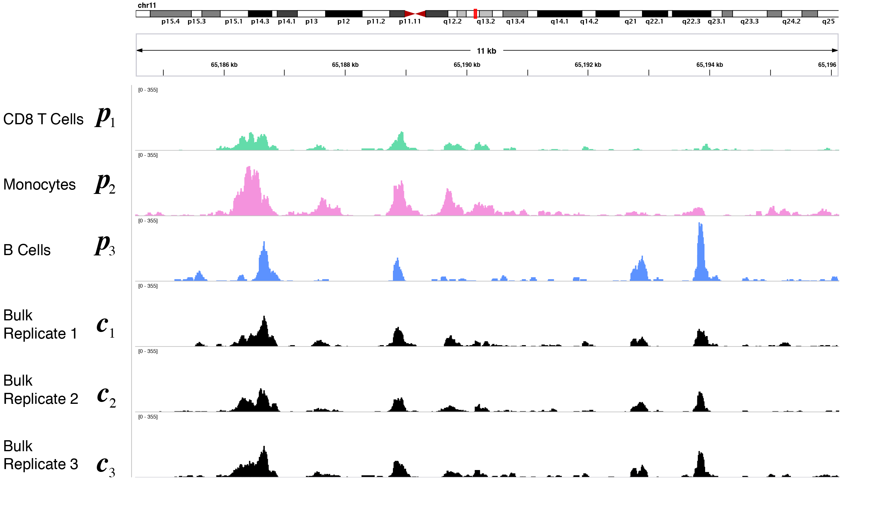
Figure 13: Epigenetic (ATAC-seq) data visualized for the three cell types used in section 7 showing an example region with differential peak heights $\boldsymbol{p}_{k}$s across the cell types and examples of simulated bulk data $\boldsymbol{c}_{t}$ for $t=1,2,3$ from the weighted sum.

Appendix B Extended Theory

Lemma 1 The epigenetic model $f(\boldsymbol{c}|\boldsymbol{p}_{k},\pi_{k})$ is non-identifiable
Proof sketch. Due to having $Kl+K$ unknowns in the mean parameters while having an $l$ dimensional Normal distribution, where $K$ is the maximum number of allowed clusters, we have an under-determined problem. Thus, we can provide multiple parameter sets $\pi_{k}$ and $\boldsymbol{p}_{k}$ leading to the same Normal distribution for $\boldsymbol{c}$.

Lemma 3 Square of a symmetric matrix $H$ gives a symmetric positive semi-definite matrix $L$.
Proof. We show that there exists a symmetric positive semi-definite matrix $L$ iff there exists a symmetrix matrix $H$ that satisfies $H^{2}=L$. $H,L\in\mathrm{R^{d\times d}}$. Orthogonal diagonalization of $L$ gives $QLQ^{-1}=D^{2}$ where $Q$ is the orthogonal matrix and $D$ is the square root diagonal matrix $diag(l_{1}^{\frac{1}{2}},\cdots,l_{d}^{\frac{1}{2}})$. If there exists a matrix $H$ where $H=Q*diag(l_{1}^{\frac{1}{2}},\cdots,l_{d}^{\frac{1}{2}})*Q^{-1}=QDQ^{-1}$, then $QHQ^{-1}=D$. We now write:

$$\begin{split}QLQ^{-1}&=D^{2}\\ &=diag(l_{1}^{\frac{1}{2}},\cdots,l_{d}^{\frac{1}{2}})*diag(l_{1}^{\frac{1}{2}},\cdots,l_{d}^{\frac{1}{2}})\\ &=QHQ^{-1}QHQ^{-1}=QH^{2}Q^{-1}\\ \end{split}$$

showing $H^{2}=L$. Next assume $H$ is symmetric and therefore all its eigenvalues are real. For some eigenvalue $h$ of $H$, $l$ is an eigenvalue of $L$ iff $l=h^{2}$ implying all eigenvalues of $L\in\mathrm{R}^{*}$ where $\mathrm{R}^{*}=\{0\}\cup\mathrm{R}^{+}$. Further, $L$ is symmetric given $H$ is symmetric. We now have $L$ as symmetric and has non-negative eigenvalues proving that $L$ is positive semi-definite. $\blacksquare$

Lemma 4 In the reduced model: $f(X^{0},C|\boldsymbol{\beta},\boldsymbol{\mu}_{k}^{0},\Sigma_{k}^{0},\boldsymbol{\alpha},\boldsymbol{z},\boldsymbol{p}_{k},R_{k}^{0},\pi_{k},\zeta)$, $\beta$s are identifiable under the conditions of: $\forall j:\boldsymbol{\mu}_{k}\geq\boldsymbol{\mu}^{\prime}+diag(\Sigma^{\prime})(\alpha_{j}-\nu)/\delta$ without the need for condition on $\beta$s.

Proof sketch. Using Lemma 2 and focusing on the marginal distribution $f(X^{0}|\boldsymbol{\beta},\boldsymbol{\mu}_{k}^{0},\Sigma_{k}^{0},\boldsymbol{\alpha},\boldsymbol{z},\pi_{k})$ we know that $\beta_{j}\Sigma_{k}^{0}$ and $\pi_{k}$ are identified for all $j$ and $k$. Hence, $\beta_{j}^{1/2}\Sigma\pi_{k}(\Sigma_{k}^{0})^{1/2}$ is identified. Using Lemma 3, $(R_{k}+R_{k}^{T})^{2}$ is non-negative semi definite which allows us to define $(\Sigma_{k}^{0})^{1/2}$ from the Wishart distribution.

Therefore, $\beta_{j}^{1/2}\Sigma\pi_{k}(R_{k}+R_{k}^{T})$ is identifiable. We also know that $\Sigma\pi_{k}\boldsymbol{p}_{k}$ is identified through the marginal distribution for $C$. Thus, putting the above together, it is not possible to have multiple values for $\beta_{j}$ since that would require the sum $\Sigma\pi_{k}(R_{k}+R_{k}^{T})$ to be different for two sets of parameters while each element of this sum can be written as elements of $\Sigma\pi_{k}\boldsymbol{p}_{k}$ which is identified. $\blacksquare$

Lemma 5 For a given $\boldsymbol{\beta}=\beta^{*}$, identifiability of: $f(X,C|\boldsymbol{\mu}_{k},\Sigma_{k},\boldsymbol{\alpha},\boldsymbol{\beta}=\boldsymbol{\beta}^{*},\boldsymbol{z},\boldsymbol{p}_{k},R_{k},\pi_{k},\zeta)$ is guaranteed if $\forall j:\boldsymbol{\mu}_{k}\geq\boldsymbol{\mu}^{\prime}+diag(\Sigma^{\prime})(\alpha_{j}-\nu)/\delta$.

Proof sketch. Parameters related to BISCUIT are identifiable using Lemma 2 without any of conditions on $\beta$s used in BISCUIT’s proof, since $\beta$s are all given.

It remains to show identifiability for parameters $\boldsymbol{p}_{k},R_{k},\zeta$ from integrated model on $C$. $\zeta$ is identified due to Normality of $C$. Identifiability of $\boldsymbol{p}_{k}$ will lead to identifiability of $R_{k}$. We focus on proving identifiability of $\boldsymbol{p}_{k}$.

Using the identifiability of $\Sigma_{k}$ we have $d(d-1)/2$ equations based on generation of $\Sigma_{k}$ based on $\boldsymbol{p}_{k}$. Considering that $\boldsymbol{p}_{k}$ has $l$ unknowns and the relationships are at most polynomials of degree 2, as long as $d(d-1)/2>l^{2}$ we have an overdetermined system of equations to identify $\boldsymbol{p}_{k}$ from $\Sigma_{k}$. $\blacksquare$

Theorem 6 The full model $f(X,C|\Theta)$ where $\Theta:=\{\boldsymbol{\mu}_{k},\Sigma_{k},\boldsymbol{\alpha},\boldsymbol{\beta},\boldsymbol{z},\boldsymbol{p}_{k},R_{k},\pi_{k},\zeta\}$ is identifiable if $\ \forall j:\boldsymbol{\mu}_{k}\geq\boldsymbol{\mu}^{\prime}+diag(\Sigma^{\prime})(\alpha_{j}-\nu)/\delta$.
Proof sketch. To prove identifiability of $\beta$, we use Lemma 5 on the following reduced distribution of $f(X,C|\Theta)$: $f(X^{0},C|\boldsymbol{\beta},\boldsymbol{\mu}_{k}^{0},\Sigma_{k}^{0},\boldsymbol{\alpha},\boldsymbol{z},\boldsymbol{p}_{k},R_{k}^{0},\pi_{k},\zeta)$. Given the identified $\beta$s from Lemma 5, we use Lemma 6 to conclude identifiability of the rest of the parameters of the full model $f(X,C|\Theta)$, as desired. $\blacksquare$

Appendix C Variational Inference update equation derivations

C.1 Joint distribution for X and C

We use the graphical model in Figure 4 to write down the variational inference equations for Symphony. Note that this is constructed based on conditionally-conjugate priors for $\boldsymbol{\mu}$ and $\Sigma$ and on space discretised by $\boldsymbol{z}=\{z_{1},\cdots,z_{n}\}$ where $z_{j}=\{j\},j=[1,\cdots,k]$. The joint is written based on the Markov blanket for each parameter.

$$\begin{split}p(X,C,\boldsymbol{z},\boldsymbol{\pi},\boldsymbol{\mu},\Sigma,\boldsymbol{\mu}^{\prime},\Sigma^{\prime},R,S,M,\lambda,\boldsymbol{\alpha},\boldsymbol{\beta},\boldsymbol{p},\eta,\gamma,\Lambda,\zeta)&=p(X|\boldsymbol{z},\boldsymbol{\mu},\Sigma,\boldsymbol{\alpha},\boldsymbol{\beta})p(C|\boldsymbol{p},\boldsymbol{\pi},\zeta)\\ &p(\boldsymbol{z}|\boldsymbol{\pi})p(\boldsymbol{\pi}|\boldsymbol{\varphi})\\ &p(\boldsymbol{\mu}^{\prime}|\boldsymbol{\mu}^{\prime\prime},\Sigma^{\prime\prime})p(\Sigma^{-1\prime}|\Sigma^{-1\prime\prime},d)\\ &p(\boldsymbol{\alpha}|\nu,\delta)p(\boldsymbol{\beta}|\omega,\theta)\\ &\prod_{k}p(\boldsymbol{\mu}_{k}|\boldsymbol{\mu}^{\prime},\Sigma^{\prime})p(\Sigma^{-1}_{k}|(R_{k}+R_{k}^{T})^{2},\gamma)p(R_{k}|SM\boldsymbol{p_{k}},\lambda)p(\boldsymbol{p}_{k}|\eta,\Lambda)\\ \end{split}$$ (9)

Next we expand each term in the RHS of Equation 9.

$$\begin{split}p(X|\boldsymbol{z},\boldsymbol{\mu},\Sigma,\boldsymbol{\alpha},\boldsymbol{\beta})&=\prod_{j}p(\boldsymbol{x}_{j}|z_{j},\boldsymbol{\mu},\Sigma,\alpha_{j},\beta_{j})\\ &=\prod_{j}\prod_{k}p(\boldsymbol{x}_{j}|z_{jk},\boldsymbol{\mu}_{k},\Sigma_{k},\alpha_{j},\beta_{j})^{z_{jk}}\\ &=\prod_{j}\prod_{k}\mathcal{N}(\boldsymbol{x}_{j}|\alpha_{j}\boldsymbol{\mu}_{k},\beta_{j}\Sigma_{k})^{z_{jk}}\\ \end{split}$$ (10)

$$\begin{split}p(\boldsymbol{z}|\boldsymbol{\pi})&=\prod_{j}p(z_{j}|\boldsymbol{\pi})\\ &=\prod_{j}\prod_{k}p(z_{jk}|\pi_{k})^{z_{jk}}\\ &=\prod_{j}\prod_{k}\mathrm{Mult}(z_{jk}|\pi_{k})^{z_{jk}}\\ &=\prod_{j}\prod_{k}\pi_{k}^{z_{jk}}\\ \end{split}$$ (11)

$$\begin{split}p(\boldsymbol{\pi}|\boldsymbol{\varphi})&=\mathrm{Dir}(\boldsymbol{\pi}|\varphi_{1},\cdots,\varphi_{K})\\ &=\mathrm{Dir}(\boldsymbol{\pi}|\varphi_{0})\\ &=\frac{1}{B(\varphi_{0})}\prod_{k}\pi_{k}^{\varphi_{0}-1}\end{split}$$ (12)

where $\sum_{k}\pi_{k}=1\quad\text{and}\quad\varphi_{1}=\cdots=\varphi_{K}$ for symmetric prior. .

In the experiments, we used:

$$\begin{split}p(\boldsymbol{\pi}|\varphi)&=\mathrm{Stick}(\boldsymbol{\pi}|\varphi)\\ p(\pi_{k}^{\prime}|\varphi)&=\mathrm{Beta}(\pi_{k}^{\prime}|1,\varphi)\\ \pi_{k}&=\pi_{k}^{\prime}\prod_{i}^{K-1}(1-\pi_{i}^{\prime})\\ \end{split}$$ (13)

where $\sum_{k}\pi_{k}=1$ and $\pi_{k}$ is the length of the k-th stick / proportion of the k-th cluster in stick breaking.

$$\begin{split}p(C|\boldsymbol{p},\boldsymbol{\pi},\zeta)&=\prod_{t}^{r}p(c_{t}|\boldsymbol{p},\boldsymbol{\pi},\zeta)\\ &=\prod_{t}^{r}\sum_{k}p(c_{t}|\boldsymbol{p},\boldsymbol{\pi},\zeta)\\ &=\prod_{t}^{r}\sum_{k}\mathcal{N}(c_{t}|\pi_{k}p_{k},\zeta\mathrm{I})\\ \end{split}$$ (14)

$$\begin{split}p(\boldsymbol{\mu}^{\prime}|\boldsymbol{\mu}^{\prime\prime},\Sigma^{\prime\prime})&=\mathcal{N}(\boldsymbol{\mu}^{\prime}|\boldsymbol{\mu}^{\prime\prime},\Sigma^{\prime\prime})\\ \end{split}$$ (15)

$$\begin{split}p(\Sigma^{\prime-1}|\Sigma^{\prime\prime-1},d)&=\mathcal{W}(\Sigma^{\prime-1}|\Sigma^{\prime\prime-1},d)\\ \end{split}$$ (16)

$$\begin{split}p(\boldsymbol{\alpha}|\nu,\delta)&=\prod_{j}p(\alpha_{j}|\nu,\delta)\\ &=\prod_{j}\mathrm{logNormal}(\alpha_{j}|\nu,\delta)\\ \end{split}$$ (17)

$$\begin{split}p(\boldsymbol{\beta}|\omega,\theta)&=\prod_{j}p(\beta_{j}|\omega,\theta)\\ &=\prod_{j}\mathrm{logNormal}(\beta_{j}|\omega,\theta)\\ \end{split}$$ (18)

$$\begin{split}\prod_{k}p(\boldsymbol{\mu}_{k}|\boldsymbol{\mu}^{\prime},\Sigma^{\prime})p(\Sigma^{-1}_{k}|R_{k},\gamma)p(R_{k}|SM\boldsymbol{p}_{k},\lambda)p(\boldsymbol{p}_{k}|\eta,\Lambda)&=\prod_{k}\mathcal{N}(\boldsymbol{\mu}_{k}|\boldsymbol{\mu}^{\prime},\Sigma^{\prime})\mathcal{W}(\Sigma^{-1}_{k}|(R_{k}+R_{k}^{T})^{2},\gamma)\\ \prod_{i}\prod_{i^{\prime}}\mathcal{N}(R_{k}^{i,i^{\prime}}|S^{i,i^{\prime}}M^{i,i^{\prime}}\boldsymbol{p}_{k}^{g(i,i^{\prime})},\lambda)\mathrm{trunc}\mathcal{N}(\boldsymbol{p_{k}}|\eta,\Lambda,\boldsymbol{0},+\infty)\\ \end{split}$$ (19)

C.2 Variational distributions

We now write the factorized distribution $q$ which will approximate the joint distribution in Equation 9. We follow Chapter 10 of Bishop (Bishop, 2006) and the Matrix cookbook Section 8.2 (Petersen et al., ).

$$\begin{split}q(\boldsymbol{z},\boldsymbol{\pi},\boldsymbol{\mu},\Sigma,\boldsymbol{\mu}^{\prime},\Sigma^{\prime},R,S,M,\lambda,\boldsymbol{\alpha},\boldsymbol{\beta},\boldsymbol{p},\eta,\gamma,\Lambda,\zeta|X,C)&=\underbrace{q(\boldsymbol{z}|X,C)}_{Variational\,\,E-step}\\ &\quad\underbrace{q(\boldsymbol{\pi},\boldsymbol{\mu},\Sigma,\boldsymbol{\mu}^{\prime},\Sigma^{\prime},R,S,M,\lambda,\boldsymbol{\alpha},\boldsymbol{\beta},\boldsymbol{p},\eta,\gamma,\Lambda,\zeta|X,C)}_{Variational\,\,M-step}\\ \end{split}$$ (20)

The sequential update equations can be written in terms of the E-step and M-step as follows:

Variational E-step.

Take the expectation of the log of the joint distribution with respect to $\boldsymbol{\Theta}:=\{\boldsymbol{\pi},\boldsymbol{\mu},\Sigma,\boldsymbol{\mu}^{\prime},\Sigma^{\prime},R,S,M,\lambda,\boldsymbol{\alpha},\boldsymbol{\beta},\boldsymbol{p},\eta,\gamma,\Lambda,\zeta\}$ i.e. all other parameters except $\boldsymbol{z}$. We have:

$$\begin{split}\ln q^{*}(\boldsymbol{z}|X,C)&=\mathbb{E}_{\boldsymbol{\Theta}}[\ln p(X,C,\boldsymbol{\pi},\boldsymbol{\mu},\Sigma,\boldsymbol{\mu}^{\prime},\Sigma^{\prime},R,S,M,\lambda,\boldsymbol{\alpha},\boldsymbol{\beta},\boldsymbol{p},\eta,\gamma,\Lambda,\zeta\ )]+Const\\ &=\mathbb{E}_{\boldsymbol{\Theta}}[\ln p(X|\boldsymbol{z},\boldsymbol{\mu},\Sigma,\boldsymbol{\alpha},\boldsymbol{\beta})+p(C|\boldsymbol{p},\boldsymbol{\pi},\zeta)+\ln p(\boldsymbol{z}|\boldsymbol{\pi})+\ln p(\boldsymbol{\pi}|\boldsymbol{\varphi})+\\ &\ln p(\boldsymbol{\mu}^{\prime}|\boldsymbol{\mu}^{\prime\prime},\Sigma^{\prime\prime})+\ln p(\Sigma^{-1\prime}|\Sigma^{-1\prime\prime},d)+\\ &\ln p(\boldsymbol{\alpha}|\nu,\delta)+\ln p(\boldsymbol{\beta}|\omega,\theta)]+\\ &\sum_{k}\Big{(}\ln p(\boldsymbol{\mu}_{k}|\boldsymbol{\mu}^{\prime},\Sigma^{\prime})+\ln p(\Sigma^{-1}_{k}|(R_{k}+R_{k}^{T})^{2},\gamma)+\ln p(R_{k}|SM\boldsymbol{p_{k}},\lambda)+\ln p(\boldsymbol{p}_{k}|\eta,\Lambda)\Big{)}]+Const\end{split}$$ (21)

Taking terms in $\boldsymbol{z}$ alone:

$$\begin{split}\ln q^{*}(\boldsymbol{z}|X,C)&=\mathbb{E}_{\boldsymbol{\Theta}}[\ln p(X|\boldsymbol{z},\boldsymbol{\mu},\Sigma,\boldsymbol{\alpha},\boldsymbol{\beta})+\ln p(\boldsymbol{z}|\boldsymbol{\pi})]+Const\\ &=\mathbb{E}_{\boldsymbol{\Theta}}[\ln\prod_{j}\prod_{k}\mathcal{N}(\boldsymbol{x}_{j}|\alpha_{j}\boldsymbol{\mu}_{k},\beta_{j}\Sigma_{k})^{z_{jk}}+\ln\prod_{j}\prod_{k}\pi_{k}^{z_{jk}}]+Const\\ &=\mathbb{E}_{\boldsymbol{\Theta}}[\sum_{j}\sum_{k}z_{jk}\ln\mathcal{N}(\boldsymbol{x}_{j}|\alpha_{j}\boldsymbol{\mu}_{k},\beta_{j}\Sigma_{k})+\sum_{j}\sum_{k}z_{jk}\ln\pi_{k}]+Const\\ &=\mathbb{E}_{\boldsymbol{\Theta}}[\sum_{j}\sum_{k}z_{jk}[\ln\mathcal{N}(\boldsymbol{x}_{j}|\alpha_{j}\boldsymbol{\mu}_{k},\beta_{j}\Sigma_{k})+\ln\pi_{k}]]+Const\\ &=\mathbb{E}_{\boldsymbol{\Theta}}[\sum_{j}\sum_{k}z_{jk}[(-\frac{d}{2}\ln 2\pi+\frac{1}{2}\ln|\beta_{j}\Sigma_{k}|^{-1}-\frac{1}{2}(\boldsymbol{x}_{j}-\alpha_{j}\boldsymbol{\mu}_{k})^{T}(\beta_{j}\Sigma_{k})^{-1}(\boldsymbol{x}_{j}-\alpha_{j}\boldsymbol{\mu}_{k}))+\ln\pi_{k}]]+Const\\ &=\sum_{j}\sum_{k}z_{jk}[\mathbb{E}_{\boldsymbol{\Theta}}(-\frac{d}{2}\ln 2\pi)+\mathbb{E}_{\boldsymbol{\Theta}}(\frac{1}{2}\ln|\beta_{j}\Sigma_{k}|^{-1})\\ &-\mathbb{E}_{\boldsymbol{\Theta}}(\frac{1}{2}(\boldsymbol{x}_{j}-\alpha_{j}\boldsymbol{\mu}_{k})^{T}(\beta_{j}\Sigma_{k})^{-1}(\boldsymbol{x}_{j}-\alpha_{j}\boldsymbol{\mu}_{k}))+\mathbb{E}_{\boldsymbol{\Theta}}(\ln\pi_{k})]+Const\\ &=\sum_{j}\sum_{k}z_{jk}\ln\Delta_{jk}+Const\\ &\propto\sum_{j}\sum_{k}z_{jk}\ln\Delta_{jk}\end{split}$$ (22)

Taking exponentials on both sides of Equation 22:

$$\begin{split}q^{*}(\boldsymbol{z}|X,C)&\propto\prod_{j}\prod_{k}\Delta_{jk}^{z_{jk}}\end{split}$$ (23)

where

$$\ln\Delta_{jk}:=-\frac{d}{2}\ln 2\pi+\underbrace{\mathbb{E}_{\boldsymbol{\Theta}}(\frac{1}{2}\ln|\beta_{j}\Sigma_{k}|^{-1})}_{S1}-\underbrace{\mathbb{E}_{\boldsymbol{\Theta}}(\frac{1}{2}(\boldsymbol{x}_{j}-\alpha_{j}\boldsymbol{\mu}_{k})^{T}(\beta_{j}\Sigma_{k})^{-1}(\boldsymbol{x}_{j}-\alpha_{j}\boldsymbol{\mu}_{k}))}_{S2}+\underbrace{\mathbb{E}_{\boldsymbol{\Theta}}(\ln\pi_{k})}_{S3}$$ (24)

Let us now expand the expectations given as S1, S2 and S3 in Equation 24.

1. $$\begin{split}S1&:=\mathbb{E}_{\boldsymbol{\Theta}}(\frac{1}{2}\ln|\beta_{j}\Sigma_{k}|^{-1})\\ &=\frac{1}{2}\mathbb{E}_{(\beta_{j},\Sigma_{k})}(\ln|\beta_{j}\Sigma_{k}|^{-1})\\ &=\frac{1}{2}\mathbb{E}_{(\beta_{j},\Sigma_{k})}(\ln\beta_{j}^{-d}|\Sigma_{k}^{-1}|)\\ &=\frac{1}{2}\mathbb{E}_{(\beta_{j},\Sigma_{k})}(\ln\beta_{j}^{-d}+\ln|\Sigma_{k}^{-1}|)\\ &=\frac{1}{2}(\mathbb{E}_{(\beta_{j},\Sigma_{k})}\ln\beta_{j}^{-d}+\mathbb{E}_{(\beta_{j},\Sigma_{k})}\ln|\Sigma_{k}^{-1}|)\\ &=\frac{1}{2}(-d\mathbb{E}_{\beta_{j}}\ln\beta_{j}+\mathbb{E}_{\Sigma_{k}}\ln|\Sigma_{k}|)\\ &=\frac{1}{2}(-d\mathbb{E}_{\beta_{j}}\ln\beta_{j}+d\ln(2)+\ln|(\boldsymbol{R}_{k}+\boldsymbol{R}_{k}^{t})^{2}|+\sum_{i=1}^{d}\psi\Big{(}\frac{\gamma_{k}+1-i}{2}\Big{)})\\ &\equiv\ln\widetilde{|\beta_{j}\Sigma_{k}|^{-1}}\\ \end{split}$$ (25)

   where $\psi(.)$ is the digamma function and equals $\tfrac{d}{dx}\log\Gamma(x)$ and $\gamma_{k}:=\gamma+n_{k}$. Runtime complexity$\sim\mathrm{O}(d^{3})$

2. $$\begin{split}S_{2}&:=\mathbb{E}_{\boldsymbol{\Theta}}[\frac{1}{2}(\boldsymbol{x}_{j}-\alpha_{j}\boldsymbol{\mu}_{k})^{T}(\beta_{j}\Sigma_{k})^{-1}(\boldsymbol{x}_{j}-\alpha_{j}\boldsymbol{\mu}_{k})]\\ &=\mathbb{E}_{(\Sigma_{k},\beta_{j},\alpha_{j},\mu_{k})}[\frac{1}{2}(\boldsymbol{x}_{j}-\alpha_{j}\boldsymbol{\mu}_{k})^{T}(\beta_{j}\Sigma_{k})^{-1}(\boldsymbol{x}_{j}-\alpha_{j}\boldsymbol{\mu}_{k})]\\ &=\tfrac{1}{2}\sum_{i}\sum_{j}(\beta\Sigma_{k_{ij}})^{-1}\mathbb{E}[(\boldsymbol{x}_{j}-\alpha_{j}\boldsymbol{\mu}_{k})^{T}(\boldsymbol{x}_{j}-\alpha_{j}\boldsymbol{\mu}_{k})]\quad\text{(linearity of expectation property)}\\ &=\tfrac{1}{2}\sum_{i}\sum_{j}(\beta\Sigma_{k_{ij}})^{-1}(\Sigma^{\prime\prime-1}+(\boldsymbol{\mu}^{\prime\prime}-\alpha_{j}\boldsymbol{\mu}_{k})^{T}(\boldsymbol{\mu}^{\prime\prime}-\alpha_{j}\boldsymbol{\mu}_{k}))\quad\text{(via covariance formula)}\\ &=\tfrac{1}{2}\sum_{i}\sum_{j}(\beta\Sigma_{k_{ij}})^{-1}(\Sigma^{\prime\prime-1})+\tfrac{1}{2}\sum_{i}\sum_{j}(\beta\Sigma_{k_{ij}})^{-1}(\boldsymbol{\mu}^{\prime\prime}-\alpha_{j}\boldsymbol{\mu}_{k})^{T}(\boldsymbol{\mu}^{\prime\prime}-\alpha_{j}\boldsymbol{\mu}_{k})\quad\text{($\Sigma_{k}$ symmetricity)}\\ &=\tfrac{1}{2}\Big{(}\textit{trace}(\Sigma_{k}^{-1}\beta^{-1}\Sigma^{\prime\prime-1})+(\boldsymbol{\mu}^{\prime\prime}-\alpha_{j}\boldsymbol{\mu}_{k})^{T}(\beta\Sigma_{k})^{-1}(\boldsymbol{\mu}^{\prime\prime}-\alpha_{j}\boldsymbol{\mu}_{k})\Big{)}\\ \end{split}$$ (26)

   Runtime complexity$\sim\mathrm{O}(d^{3})$

3. $$\begin{split}S3&:=\mathbb{E}_{\boldsymbol{\Theta}}[\ln\pi_{k}]\\ &=\mathbb{E}_{\boldsymbol{\pi}}[\ln\pi_{k}]\\ &=\psi(\varphi_{0})-\psi(\sum_{k}\varphi_{k})\\ &\equiv\ln\widetilde{\pi}_{k}\end{split}$$ (27)

   where $\psi$ is the digamma function and $\psi(t)=\frac{d}{d_{0}}\ln(\Gamma(t))=\frac{\Gamma^{\prime}(t)}{\Gamma(t)}$. Runtime complexity$\sim\mathrm{O}(1)$

Therefore,

$$\ln\Delta_{jk}:=-\frac{d}{2}\ln 2\pi+\ln\widetilde{|\beta_{j}\Sigma_{k}|^{-1}}-\mathbb{E}_{\boldsymbol{\Theta}}[\frac{1}{2}(\boldsymbol{x}_{j}-\alpha_{j}\boldsymbol{\mu}_{k})^{T}(\beta_{j}\Sigma_{k})^{-1}(\boldsymbol{x}_{j}-\alpha_{j}\boldsymbol{\mu}_{k})]+\ln\widetilde{\pi}_{k}$$ (28)

We require that $q^{*}(\boldsymbol{z}|X)$ is normalised and that for every observation $j$, there is only one non-zero $z_{jk}$ $\forall$ $k\in\{1,\cdots,K\}$. Therefore it is sufficient to normalise each $\Delta_{jk}$ as

$$r_{jk}=\frac{\Delta_{jk}}{\sum_{h=1}^{K}\Delta_{jh}}$$ (29)

$$\begin{split}q^{*}(\boldsymbol{z}|X)&=\prod_{j}\prod_{k}r_{jk}^{z_{jk}}\\ &=\prod_{j}q^{*}(z_{j})\\ \end{split}$$ (30)

The expectation for the discrete distribution $q^{*}(z_{jk})$ gives the responsibilities $r_{jk}$ for point $x_{j}$ with the current $k^{th}$ cluster’s parameters :

$$\begin{split}\mathbb{E}_{q^{*}(z_{jk})}[z_{jk}]&:=\frac{\pi_{k}\mathcal{N}(\boldsymbol{x}_{j}|\alpha_{j}\boldsymbol{\mu}_{k},\beta_{j}\Sigma_{k})}{\sum_{m=1}^{K}\pi_{m}\mathcal{N}(\boldsymbol{x}_{j}|\alpha_{j}\boldsymbol{\mu}_{m},\beta_{j}\Sigma_{m})}=r_{jk}\\ \end{split}$$ (31)

with the overall runtime complexity for calculating $r_{jk}$ is $\mathrm{O}(d^{3})$.

MAP estimate for z

Since the E-step has a runtime $\sim\mathrm{O}(d^{3})$ due to three matrix inversions, we substitute this as $z_{MAP}(\boldsymbol{x})=\arg\max_{z}p(\boldsymbol{x}|\boldsymbol{z})p(\boldsymbol{z}|\boldsymbol{\pi})$ which has a runtime of $\sim\mathrm{O}(d^{2})$ when $\Sigma_{k}^{-1}$s and $\Sigma^{\prime\prime}$ are apriori Cholesky decomposed.

Variational M-step.

Take the expectation of the log of the joint distribution with respect to $\boldsymbol{z}$. We have:

$$\begin{split}\ln q^{*}(&\boldsymbol{\pi},\boldsymbol{\mu},\Sigma,\boldsymbol{\mu}^{\prime},\Sigma^{\prime},R,S,M,\lambda,\boldsymbol{\alpha},\boldsymbol{\beta},\boldsymbol{p},\eta,\gamma,\Lambda,\zeta|X,C)\\ &=\mathbb{E}_{\boldsymbol{z}}[\ln p(X,C,\boldsymbol{z},\boldsymbol{\pi},\boldsymbol{\mu},\Sigma,\boldsymbol{\mu}^{\prime},\Sigma^{\prime},R,S,M,\lambda,\boldsymbol{\alpha},\boldsymbol{\beta},\boldsymbol{p},\eta,\gamma,\Lambda,\zeta)]+C\\ &=\mathbb{E}_{\boldsymbol{z}}[\ln p(X|\boldsymbol{z},\boldsymbol{\mu},\Sigma,\boldsymbol{\alpha},\boldsymbol{\beta})+\ln p(C|\boldsymbol{p},\boldsymbol{\pi},\zeta)+\ln p(\boldsymbol{z}|\boldsymbol{\pi})+\ln p(\boldsymbol{\pi}|\boldsymbol{\varphi})+\\ &\ln p(\boldsymbol{\mu}^{\prime}|\boldsymbol{\mu}^{\prime\prime},\Sigma^{\prime\prime})+\ln p(\Sigma^{-1\prime}|\Sigma^{-1\prime\prime},d)+\\ &\ln p(\boldsymbol{\alpha}|\nu,\delta)+\ln p(\boldsymbol{\beta}|\omega,\theta)]+\\ &\sum_{k}\Big{(}\ln p(\boldsymbol{\mu}_{k}|\boldsymbol{\mu}^{\prime},\Sigma^{\prime})+\ln p(\Sigma^{-1}_{k}|\boldsymbol{R}_{k},\gamma)+\ln p(\boldsymbol{R}_{k}|SM\boldsymbol{p_{k}},\lambda)+\ln p(\boldsymbol{p}_{k}|\eta,\Lambda)\Big{)}]+Const\end{split}$$ (32)

Taking terms in $(\boldsymbol{\pi},\boldsymbol{\mu},\Sigma,\boldsymbol{\mu}^{\prime},\Sigma^{\prime},R,S,M,\lambda,\boldsymbol{\alpha},\boldsymbol{\beta},\boldsymbol{p},\eta,\gamma,\Lambda,\zeta)$, we get:

$$\begin{split}\ln&q^{*}(\boldsymbol{\pi},\boldsymbol{\mu},\Sigma,\boldsymbol{\mu}^{\prime},\Sigma^{\prime},R,S,M,\lambda,\boldsymbol{\alpha},\boldsymbol{\beta},\boldsymbol{p},\eta,\gamma,\Lambda|X,C)=\\ &\mathbb{E}_{\boldsymbol{z}}[\ln p(X|\boldsymbol{z},\boldsymbol{\mu},\Sigma,\boldsymbol{\alpha},\boldsymbol{\beta})+\\ &\ln p(\boldsymbol{z}|\boldsymbol{\pi})+\ln p(C|\boldsymbol{p},\boldsymbol{\pi},\zeta)+\ln p(\boldsymbol{\pi}|\boldsymbol{\varphi})+\\ &\ln p(\boldsymbol{\mu}^{\prime}|\boldsymbol{\mu}^{\prime\prime},\Sigma^{\prime\prime})+\ln p(\Sigma^{-1\prime}|\Sigma^{-1\prime\prime},d)+\ln p(\boldsymbol{\alpha}|\nu,\delta)+\ln p(\boldsymbol{\beta}|\omega,\theta)]+\\ &\sum_{k}\Big{(}\ln p(\boldsymbol{\mu}_{k}|\boldsymbol{\mu}^{\prime},\Sigma^{\prime})+\ln p(\Sigma^{-1}_{k}|(R_{k}+R_{k}^{T})^{2},\gamma)+\ln p(R_{k}|SM\boldsymbol{p_{k}},\lambda)+\ln p(\boldsymbol{p}_{k}|\eta,\Lambda)\Big{)}]\\ &+C\\ &=\mathbb{E}_{\boldsymbol{z}}\Big{[}\ln\prod_{j}\prod_{k}\mathcal{N}(\boldsymbol{x}_{j}|\alpha_{j}\boldsymbol{\mu}_{k},\beta_{j}\Sigma_{k})^{z_{jk}}+\ln\prod_{j}\prod_{k}\pi_{k}^{z_{jk}}\Big{]}+\ln\mathrm{Dir}(\boldsymbol{\pi}|\varphi_{0})+\\ &\ln\prod_{t}^{r}\prod_{k}\mathcal{N}(c_{t}|\sum_{k}\pi_{k}\boldsymbol{p}_{k},\zeta\mathrm{I})+\ln\mathcal{N}(\boldsymbol{\mu}^{\prime}|\boldsymbol{\mu}^{\prime\prime},\Sigma^{\prime\prime})+\ln\mathcal{W}(\Sigma^{\prime-1}|\Sigma^{\prime\prime-1},d)+\\ &\ln\prod_{j}\mathrm{logNormal}(\alpha_{j}|\nu,\delta)+\ln\prod_{j}\mathrm{logNormal}(\beta_{j}|\omega,\theta)+\\ &\ln\Big{(}\prod_{k}\mathcal{N}(\boldsymbol{\mu}_{k}|\boldsymbol{\mu}^{\prime},\Sigma^{\prime})\mathrm{Wishart}(\Sigma^{-1}_{k}|R_{k},\gamma)\mathcal{N}((R_{k}+R_{k}^{T})^{2}|SM\boldsymbol{p}_{k},\lambda)\mathrm{trunc}\mathcal{N}(\boldsymbol{p}_{k}|\eta,\Lambda)\Big{)}\\ &+Const\\ &=\mathbb{E}_{\boldsymbol{z}}\Big{[}\sum_{j}\sum_{k}z_{jk}\ln\mathcal{N}(\boldsymbol{x}_{j}|\alpha_{j}\boldsymbol{\mu}_{k},\beta_{j}\Sigma_{k})+\sum_{j}\sum_{k}z_{jk}\ln\pi_{k}\Big{]}+\ln\mathrm{Dir}(\boldsymbol{\pi}|\varphi_{0})+\\ &\sum_{t}^{r}\sum_{k}\ln\mathcal{N}(c_{t}|\sum_{k}\pi_{k}\boldsymbol{p}_{k},\zeta\mathrm{I})+\ln\mathcal{N}(\boldsymbol{\mu}^{\prime}|\boldsymbol{\mu}^{\prime\prime},\Sigma^{\prime\prime})+\ln\mathcal{W}(\Sigma^{\prime-1}|\Sigma^{\prime\prime-1},d)+\\ &\sum_{j}\ln\mathrm{logNormal}(\alpha_{j}|\nu,\delta)+\sum_{j}\ln\mathrm{logNormal}(\beta_{j}|\omega,\theta)+\\ &\sum_{k}\ln\mathcal{N}(\boldsymbol{\mu}_{k}|\boldsymbol{\mu}^{\prime},\Sigma^{\prime})+\sum_{k}\ln\mathrm{Wishart}(\Sigma^{-1}_{k}|(R_{k}+R_{k}^{T})^{2},\gamma)+\\ &\sum_{k}\ln\mathcal{N}(R_{k}|SM\boldsymbol{p}_{k},\lambda)+\sum_{k}\ln\mathrm{trunc}\mathcal{N}(\boldsymbol{p}_{k}|\eta,\Lambda)+Const\\ \end{split}$$ (33)

We assume that the set of latent variables is independent of the rest of the latent variables given $X$ and $C$. This independence assumption reduces the problem complexity and allows us to get closed-form solutions in the M-step. This is called the mean-field assumption. We use this assumption and proceed to factor the latent variables into conditionally-independent components, to perform co-ordinate ascent mean field VI (CAVI) on each variational component:

$$\begin{split}\ln&q^{*}(\boldsymbol{\pi},\boldsymbol{\mu},\Sigma,\boldsymbol{\mu}^{\prime},\Sigma^{\prime},R,S,M,\lambda,\boldsymbol{\alpha},\boldsymbol{\beta},\boldsymbol{p},\eta,\gamma,\Lambda,\zeta|X,C)\\ &=\ln q^{*}(\boldsymbol{\pi})+\ln q^{*}(\boldsymbol{\mu})+\ln q^{*}(\Sigma)+\ln q^{*}(\boldsymbol{\alpha})+\ln q^{*}(\boldsymbol{\beta})\\ &+\ln q^{*}(\boldsymbol{\mu}^{\prime})++\ln q^{*}(\Sigma^{\prime})+\ln q^{*}(R)+\ln q^{*}(\boldsymbol{p})\\ &=\ln q^{*}(\boldsymbol{\pi})+\ln\prod_{k}q^{*}(\mu_{k})+\ln\prod_{k}q^{*}(\Sigma_{k}^{-1})+\ln\prod_{j}q^{*}(\alpha_{j})+\ln\prod_{j}q^{*}(\beta_{j})\\ &+\ln q^{*}(\boldsymbol{\mu}^{\prime})++\ln q^{*}(\Sigma^{\prime})+\ln\prod_{k}q^{*}(R)+\ln\prod_{k}q^{*}(\boldsymbol{p})\\ &=\ln q^{*}(\boldsymbol{\pi})+\sum_{k}\ln q^{*}(\mu_{k})+\sum_{k}\ln q^{*}(\Sigma_{k}^{-1})+\sum_{j}\ln q^{*}(\alpha_{j})+\sum_{j}\ln q^{*}(\beta_{j})\\ &+\ln q^{*}(\boldsymbol{\mu}^{\prime})++\ln q^{*}(\Sigma^{\prime})+\sum_{k}\ln q^{*}(R)+\sum_{k}\ln q^{*}(\boldsymbol{p})\\ \end{split}$$ (34)

Let us find the approximate distributions $q^{*}(\cdot)$ for every parameter in the RHS of Equation 34 by comparing to RHS of Equation 33.

1. $$\begin{split}q^{*}(\boldsymbol{\pi})=p(\boldsymbol{\pi}|\varphi)&=\mathrm{Stick}(\boldsymbol{\pi}|\varphi)\\ p(\pi_{k}^{\prime}|\varphi)&=\mathrm{Beta}(\pi_{k}^{\prime}|1,\varphi)\\ \pi_{k}&=\pi_{k}^{\prime}\prod_{i}^{K-1}(1-\pi_{i}^{\prime})\\ \end{split}$$ (35)

2. $$\begin{split}\sum_{k}\ln q^{*}(\mu_{k})&=\mathbb{E}_{\boldsymbol{z}}\Big{[}\sum_{j}\sum_{k}{z_{jk}}\ln\mathcal{N}(\boldsymbol{x}_{j}|\alpha_{j}\boldsymbol{\mu}_{k},\beta_{j}\Sigma_{k})\Big{]}+\sum_{k}\ln\mathcal{N}(\boldsymbol{\mu}_{k}|\boldsymbol{\mu}^{\prime},\Sigma^{\prime})\\ &=\sum_{k}\underbrace{(\mathbb{E}_{\boldsymbol{z}}\Big{[}\sum_{j}{z_{jk}}\ln\mathcal{N}(\boldsymbol{x}_{j}|\alpha_{j}\boldsymbol{\mu}_{k},\beta_{j}\Sigma_{k})\Big{]}+\ln\mathcal{N}(\boldsymbol{\mu}_{k}|\boldsymbol{\mu}^{\prime},\Sigma^{\prime}))}_{expanded\,\,below}\\ &=\sum_{j}\mathbb{E}_{\boldsymbol{z}}{z_{jk}}\ln\mathcal{N}(\boldsymbol{x}_{j}|\alpha_{j}\boldsymbol{\mu}_{k},\beta_{j}\Sigma_{k})+\ln\mathcal{N}(\boldsymbol{\mu}_{k}|\boldsymbol{\mu}^{\prime},\Sigma^{\prime})\\ &=-\frac{1}{2}\sum_{j}\mathbb{E}_{\boldsymbol{z}}{z_{jk}}(\boldsymbol{\mu}_{k}-\frac{\boldsymbol{x}_{j}}{\alpha_{j}})^{T}{(\frac{\beta_{j}}{\alpha_{j}^{2}}\Sigma_{k})}^{-1}(\boldsymbol{\mu}_{k}-\frac{x_{j}}{\alpha_{j}})\\ &-\frac{1}{2}\sum_{j}\mathbb{E}_{\boldsymbol{z}}{z_{jk}}\ln|\beta_{j}\Sigma_{k}|-\frac{d}{2}\sum_{j}\mathbb{E}_{\boldsymbol{z}}{z_{jk}}\ln(2\pi)\\ &-\frac{1}{2}\ln|\Sigma^{\prime}|-\frac{d}{2}\ln(2\pi)-\frac{1}{2}(\boldsymbol{\mu}_{k}-\boldsymbol{\mu}^{\prime})^{T}\Sigma^{\prime-1}(\boldsymbol{\mu}_{k}-\boldsymbol{\mu}^{\prime})\\ &\propto-\frac{1}{2}\sum_{j}\mathbb{E}_{\boldsymbol{z}}[{z_{jk}}(\boldsymbol{\mu}_{k}-\frac{\boldsymbol{x}_{j}}{\alpha_{j}})^{T}{(\frac{\beta_{j}}{\alpha_{j}^{2}}\Sigma_{k})}^{-1}(\boldsymbol{\mu}_{k}-\frac{\boldsymbol{x}_{j}}{\alpha_{j}})]-\frac{1}{2}(\boldsymbol{\mu}_{k}-\boldsymbol{\mu}^{\prime})^{T}\Sigma^{\prime-1}(\boldsymbol{\mu}_{k}-\boldsymbol{\mu}^{\prime})\\ &\text{(by taking terms in $\mu_{k}$ and $\mu^{\prime}$)}\\ &\propto-\frac{1}{2}\sum_{j}\mathbb{E}_{\boldsymbol{z}}{z_{jk}}\mathbb{E}_{\boldsymbol{z}}[(\boldsymbol{\mu}_{k}-\frac{\boldsymbol{x}_{j}}{\alpha_{j}})^{T}{(\frac{\beta_{j}}{\alpha_{j}^{2}}\Sigma_{k})}^{-1}(\boldsymbol{\mu}_{k}-\frac{\boldsymbol{x}_{j}}{\alpha_{j}})]-\frac{1}{2}(\boldsymbol{\mu}_{k}-\boldsymbol{\mu}^{\prime})^{T}\Sigma^{\prime-1}(\boldsymbol{\mu}_{k}-\boldsymbol{\mu}^{\prime})\\ &\propto-\frac{1}{2}\sum_{j}\mathbb{E}_{\boldsymbol{z}}{z_{jk}}\Big{(}\textit{trace(}\Sigma_{k}^{-1}(\tfrac{\beta_{j}}{\alpha_{j}^{2}})^{-1}\Sigma^{\prime\prime-1})+(\boldsymbol{\bar{\mu}_{k}}-\frac{\boldsymbol{x}_{j}}{\alpha_{j}})^{T}{(\frac{\beta_{j}}{\alpha_{j}^{2}}\Sigma_{k})}^{-1}(\boldsymbol{\bar{\mu}_{k}}-\frac{\boldsymbol{x}_{j}}{\alpha_{j}})\Big{)}\\ &-\frac{1}{2}(\boldsymbol{\mu}_{k}-\boldsymbol{\mu}^{\prime})^{T}\Sigma^{\prime-1}(\boldsymbol{\mu}_{k}-\boldsymbol{\mu}^{\prime})\\ &\propto-\frac{1}{2}\sum_{k}\Big{(}\sum_{j}r_{jk}\Big{(}\textit{trace}(\Sigma_{k}^{-1}(\tfrac{\beta_{j}}{\alpha_{j}^{2}})^{-1}\Sigma^{\prime\prime-1})+(\boldsymbol{\bar{\mu}_{k}}-\frac{\boldsymbol{x}_{j}}{\alpha_{j}})^{T}{(\frac{\beta_{j}}{\alpha_{j}^{2}}\Sigma_{k})}^{-1}(\boldsymbol{\bar{\mu}_{k}}-\frac{\boldsymbol{x}_{j}}{\alpha_{j}})\Big{)}\\ &+(\boldsymbol{\mu}_{k}-\boldsymbol{\mu}^{\prime})^{T}\Sigma^{\prime-1}(\boldsymbol{\mu}_{k}-\boldsymbol{\mu}^{\prime})\Big{)}\\ \end{split}$$ (36)

3. Let us denote $R^{*}_{k}=(R_{k}+R_{k}^{T})^{2}$. By construction of $R_{k}$, $R^{*}_{k}$ is a Gram matrix and a valid scale matrix for Wishart parametrisation.

   $$\begin{split}\sum_{k}\ln q^{*}(\Sigma_{k}^{-1})&=\mathbb{E}_{\boldsymbol{z}}\Big{[}\sum_{j}\sum_{k}{z_{jk}}\ln\mathcal{N}(\boldsymbol{x}_{j}|\alpha_{j}\boldsymbol{\mu}_{k},\beta_{j}\Sigma_{k})\Big{]}+\sum_{k}\ln\mathcal{W}(\Sigma^{-1}_{k}|R^{*}_{k},\lambda)\\ &=\sum_{k}\Big{[}\underbrace{\sum_{j}\mathbb{E}_{\boldsymbol{z}}{z_{jk}}\ln\mathcal{N}(\boldsymbol{x}_{j}|\alpha_{j}\boldsymbol{\mu}_{k},\beta_{j}\Sigma_{k})+\ln\mathcal{W}(\Sigma^{-1}_{k}|R^{*}_{k},\lambda)}_{expanded\,\,below}\Big{]}\\ &=-\sum_{j}\mathbb{E}_{\boldsymbol{z}}{z_{jk}}\frac{d}{2}\ln 2\pi-\sum_{j}\mathbb{E}_{\boldsymbol{z}}{z_{jk}}\frac{1}{2}\ln\beta_{j}^{d}-\\ &\sum_{j}\mathbb{E}_{\boldsymbol{z}}{z_{jk}}\frac{1}{2}\ln|\Sigma_{k}|-\sum_{j}\mathbb{E}_{\boldsymbol{z}}{z_{jk}}\frac{1}{2\beta_{j}}(\boldsymbol{x}_{j}-\alpha_{j}\boldsymbol{\mu}_{k})^{T}(\Sigma_{k})^{-1}(\boldsymbol{x}_{j}-\alpha_{j}\boldsymbol{\mu}_{k})+\\ &\ln|\Sigma_{k}^{-1}|^{\frac{\lambda-d-1}{2}}+\{-\frac{tr(R^{*-1}_{k}\Sigma_{k}^{-1})}{2}\}-\ln(2^{\lambda d/2}|R^{*-1}_{k}|^{-\lambda/2}\Gamma_{d}(\lambda/2))\\ &\propto-\sum_{j}\mathbb{E}_{z}z_{jk}(\tfrac{1}{2}\ln\beta_{j}^{d}+\tfrac{1}{2}\ln|\Sigma_{k}|)\\ &-\sum_{j}\mathbb{E}_{z}z_{jk}\tfrac{1}{2\beta_{j}}\Big{(}\textit{trace}(\Sigma_{k}^{-1}\Sigma^{\prime\prime-1})+(\boldsymbol{\mu}^{\prime\prime}-\alpha_{j}\boldsymbol{\mu}_{k})^{T}(\Sigma_{k})^{-1}(\boldsymbol{\mu}^{\prime\prime}-\alpha_{j}\boldsymbol{\mu}_{k})\Big{)}\\ &+\ln|\Sigma_{k}^{-1}|^{\frac{\lambda-d-1}{2}}+\{-\frac{tr(R^{*-1}_{k}\Sigma_{k}^{-1})}{2}\}-\ln(2^{\lambda d/2}|R^{*-1}_{k}|^{-\lambda/2}\Gamma_{d}(\lambda/2))\\ \end{split}$$ (37)

4. If $\alpha_{j}\sim\log\mathcal{N}(\nu,\delta)$, then $\alpha_{j}^{*}=\ln\alpha_{j}\sim\mathcal{N}(\nu,\delta)$ by properties of log Normal distribution (Aitchison & Brown, 1957).

   $$\begin{split}\sum_{j}\ln q^{*}(\alpha_{j})&=\mathbb{E}_{\boldsymbol{z}}\Big{[}\sum_{j}\sum_{k}{z_{jk}}\ln\mathcal{N}(\boldsymbol{x}_{j}|\alpha_{j}\boldsymbol{\mu}_{k},\beta_{j}\Sigma_{k})\Big{]}+\sum_{j}\ln\mathcal{N}(\alpha_{j}|\nu,\delta)\\ &=\mathbb{E}_{\boldsymbol{z}}\Big{[}\sum_{j}\sum_{k}{z_{jk}}\ln\mathcal{N}(\boldsymbol{x}_{j}|\alpha_{j}\boldsymbol{\mu}_{k},\beta_{j}\Sigma_{k})\Big{]}+\sum_{j}\mathcal{N}(\alpha_{j}^{*}|\nu,\delta)\\ &=\sum_{j}\underbrace{(\Big{[}\sum_{k}\mathbb{E}_{\boldsymbol{z}}{z_{jk}}\ln\mathcal{N}(\boldsymbol{x}_{j}|\alpha_{j}\boldsymbol{\mu}_{k},\beta_{j}\Sigma_{k})\Big{]}+\mathcal{N}(\alpha_{j}^{*}|\nu,\delta))}_{expanded\,\,below}\\ &=-\frac{1}{2}\sum_{k}\mathbb{E}_{\boldsymbol{z}}{z_{jk}}\ln|\beta_{j}\Sigma_{k}|-\frac{d}{2}\sum_{k}\mathbb{E}_{\boldsymbol{z}}{z_{jk}}\ln(2\pi)-\\ &\sum_{k}\mathbb{E}_{\boldsymbol{z}}{z_{jk}}\frac{1}{2}(\boldsymbol{x}_{j}-\alpha_{j}\boldsymbol{\mu}_{k})^{T}{(\beta_{j}\Sigma_{k})}^{-1}(\boldsymbol{x}_{j}-\alpha_{j}\boldsymbol{\mu}_{k})+\\ &\frac{1}{\sqrt{2\delta^{2}\pi}}\exp\Big{(}-\frac{(\alpha_{j}^{*}-\nu)\mathbb{I}_{1\times 1}(\alpha_{j}^{*}-\nu)}{2\delta^{2}}\Big{)}\\ &\propto-\sum_{k}\mathbb{E}_{\boldsymbol{z}}{z_{jk}}\frac{1}{2}(\boldsymbol{x}_{j}-\alpha_{j}\boldsymbol{\mu}_{k})^{T}{(\beta_{j}\Sigma_{k})}^{-1}(\boldsymbol{x}_{j}-\alpha_{j}\boldsymbol{\mu}_{k})+\\ &\frac{1}{\sqrt{2\delta^{2}\pi}}\exp\Big{(}-\frac{(\alpha_{j}^{*}-\nu)\mathbb{I}_{1\times 1}(\alpha_{j}^{*}-\nu)}{2\delta^{2}}\Big{)}\,\,\text{(taking terms in $\alpha_{j}$)}\\ &\propto-\sum_{k}r_{jk}\frac{1}{2}(\textit{trace}(\Sigma_{k}^{-1}\beta^{-1}\Sigma^{\prime\prime-1})+(\boldsymbol{\mu}^{\prime\prime}-\alpha_{j}\boldsymbol{\mu}_{k})^{T}(\beta\Sigma_{k})^{-1}(\boldsymbol{\mu}^{\prime\prime}-\alpha_{j}\boldsymbol{\mu}_{k}))+\\ &\frac{\alpha_{j}}{\alpha_{j}\sqrt{2\delta^{2}\pi}}\exp\Big{(}-\frac{(\ln\alpha_{j}-\nu)\mathbb{I}_{1\times 1}(\ln\alpha_{j}-\nu)}{2\delta^{2}}\Big{)}\,\,\\ &\text{(by replacing $\alpha_{j}^{*}$ with $\ln\alpha_{j}$ and making this a logNormal pdf )}\\ \end{split}$$ (38)

5. Derivation is similar to that of Equation 38.

   $$\begin{split}\sum_{j}\ln q^{*}(\beta_{j})&=\mathbb{E}_{\boldsymbol{z}}\Big{[}\sum_{j}\sum_{k}{z_{jk}}\ln\mathcal{N}(\boldsymbol{x}_{j}|\alpha_{j}\boldsymbol{\mu}_{k},\beta_{j}\Sigma_{k})\Big{]}+\sum_{j}\ln\mathrm{log}\mathcal{N}(\beta_{j}|\omega,\theta)\\ &=\mathbb{E}_{\boldsymbol{z}}\Big{[}\sum_{j}\sum_{k}{z_{jk}}\ln\mathcal{N}(\boldsymbol{x}_{j}|\alpha_{j}\boldsymbol{\mu}_{k},\beta_{j}\Sigma_{k})\Big{]}+\sum_{j}\mathcal{N}(\beta_{j}^{*}|\omega,\theta)\\ &\propto-\sum_{k}r_{jk}\frac{1}{2}(\textit{trace}(\Sigma_{k}^{-1}\beta^{-1}\Sigma^{\prime\prime-1})+(\boldsymbol{\mu}^{\prime\prime}-\alpha_{j}\boldsymbol{\mu}_{k})^{T}(\beta\Sigma_{k})^{-1}(\boldsymbol{\mu}^{\prime\prime}-\alpha_{j}\boldsymbol{\mu}_{k}))+\\ &\frac{\beta_{j}}{\beta_{j}\sqrt{2\theta^{2}\pi}}\exp\Big{(}-\frac{(\ln\beta_{j}-\omega)\mathbb{I}_{1\times 1}(\ln\beta_{j}-\omega)}{2\theta^{2}}\Big{)}\,\,\\ &\text{(by replacing $\beta_{j}^{*}$ with $\ln\beta_{j}$ and making this a logNormal pdf )}\\ \end{split}$$ (39)

6. $$\begin{split}\ln q^{*}(\boldsymbol{\mu}^{\prime})&=\ln\mathcal{N}(\boldsymbol{\mu}^{\prime}|\boldsymbol{\mu}^{\prime\prime},\Sigma^{\prime\prime})+\sum_{k}\ln\mathcal{N}(\boldsymbol{\mu}_{k}|\boldsymbol{\mu}^{\prime},\Sigma^{\prime})\\ &\sim\ln\mathcal{N}(\boldsymbol{\mu}_{\mu^{\prime}},\Sigma_{\mu^{\prime}})\\ \boldsymbol{\mu}_{\mu^{\prime}}&=\Sigma_{\mu^{\prime}}(\Sigma^{\prime\prime-1}\boldsymbol{\mu}^{\prime\prime}+K^{2}\Sigma^{\prime-1}\boldsymbol{\bar{\mu^{\prime}}})\\ \Sigma_{\mu^{\prime}}&=(\Sigma^{\prime\prime-1}+K\Sigma^{\prime-1})^{-1}\\ \end{split}$$ (40)

7. $$\begin{split}\ln q^{*}(\Sigma^{-1\prime})&=\ln\mathcal{W}(\Sigma^{\prime-1}|\Sigma^{\prime\prime-1},d)+\sum_{k}\ln\mathcal{N}(\boldsymbol{\mu}_{k}|\boldsymbol{\mu}^{\prime},\Sigma^{\prime})\\ &\sim\ln\mathcal{W}(V_{\Sigma^{\prime-1}},d_{\Sigma^{\prime-1}})\\ V_{\Sigma^{\prime-1}}&=(d\Sigma^{\prime\prime}+2\Sigma_{rss})^{-1}\\ d_{\Sigma^{\prime-1}}&=d+K\\ \end{split}$$ (41)

8. $$\begin{split}\sum_{k}\ln q^{*}(R_{k})&=\mathbb{E}_{(\pi_{k},\boldsymbol{p}_{k})}[\sum_{t}^{r}\sum_{k}\ln\mathcal{N}(c_{t}|\sum_{k}(\pi_{k}p_{k}),\zeta\mathbb{I})]+\sum_{k}\ln\mathcal{W}(\Sigma_{k}^{-1}|R_{k}^{*},\gamma)+\\ &\sum_{k}\sum_{i}\sum_{i^{\prime}}\ln\mathcal{N}(R_{k}^{i,i^{\prime}}|S^{i,i^{\prime}}M^{i,i^{\prime}}\boldsymbol{p}_{k}^{g(i,i^{\prime})},\lambda)\\ \ln q^{*}(R_{k})&=\mathbb{E}_{(\pi_{k},\boldsymbol{p}_{k})}[\sum_{t}^{r}\ln\mathcal{N}(c_{t}|\sum_{k}(\pi_{k}\boldsymbol{p}_{k}),\zeta\mathbb{I})]+\ln\mathcal{W}(\Sigma_{k}^{-1}|R_{k}^{*},\gamma)+\\ &\sum_{i}\sum_{i^{\prime}}\ln\mathcal{N}(R_{k}^{i,i^{\prime}}|S^{i,i^{\prime}}M^{i,i^{\prime}}\boldsymbol{p}_{k}^{g(i,i^{\prime})},\lambda)\\ &=\sum_{t}^{r}\mathbb{E}_{(\pi_{k},\boldsymbol{p}_{k})}[(c_{t}-\sum_{k}(\pi_{k}\boldsymbol{p}_{k}))^{T}(\zeta\mathbb{I})^{-1}(c_{t}-\sum_{k}(\pi_{k}\boldsymbol{p}_{k}))]+\ln\mathcal{W}(\Sigma_{k}^{-1}|R_{k}^{*},\gamma)+\\ &\sum_{i}\sum_{i^{\prime}}\ln\mathcal{N}(R_{k}^{i,i^{\prime}}|S^{i,i^{\prime}}M^{i,i^{\prime}}\boldsymbol{p}_{k}^{g(i,i^{\prime})},\lambda)\\ &\propto\sum_{t}^{r}\textit{trace}(\zeta\mathbb{I})^{-1}+(\bar{c}_{t}-\sum_{k}(\pi_{k}\boldsymbol{p}_{k}))^{T}(\zeta\mathbb{I})^{-1}(\bar{c}_{t}-\sum_{k}(\pi_{k}\boldsymbol{p}_{k}))]+\\ &\{-\frac{tr(R^{*-1}_{k}\Sigma_{k}^{-1})}{2}\}-\ln(2^{\lambda d/2}|R^{*-1}_{k}|^{-\lambda/2}\Gamma_{d}(\lambda/2))\\ &-\tfrac{1}{2\delta^{2}}\sum_{i}\sum_{i^{\prime}}\Big{(}(R_{k}^{i,i^{\prime}}-S^{i,i^{\prime}}M^{i,i^{\prime}}\boldsymbol{p}_{k}^{g(i,i^{\prime})})\mathbb{I}_{1\times 1}(R_{k}^{i,i^{\prime}}-S^{i,i^{\prime}}M^{i,i^{\prime}}\boldsymbol{p}_{k}^{g(i,i^{\prime})})\Big{)}\\ &\propto\{-\frac{tr(R^{*-1}_{k}\Sigma_{k}^{-1})}{2}\}-\ln(2^{\lambda d/2}|R^{*-1}_{k}|^{-\lambda/2}\Gamma_{d}(\lambda/2))\\ &-\tfrac{1}{2\delta^{2}}\sum_{i}\sum_{i^{\prime}}\Big{(}(R_{k}^{i,i^{\prime}}-S^{i,i^{\prime}}M^{i,i^{\prime}}\boldsymbol{p}_{k}^{g(i,i^{\prime})})\mathbb{I}_{1\times 1}(R_{k}^{i,i^{\prime}}-S^{i,i^{\prime}}M^{i,i^{\prime}}\boldsymbol{p}_{k}^{g(i,i^{\prime})})\Big{)}\quad\\ &\text{(taking terms only in $R_{k}$)}\\ \end{split}$$ (42)

9. $$\begin{split}\sum_{k}\ln q^{*}(\boldsymbol{p}_{k})&=\mathbb{E}_{(\pi_{k},\boldsymbol{p}_{k})}[\sum_{t}^{r}\sum_{k}\ln\mathcal{N}(c_{t}|\sum_{k}(\pi_{k}\boldsymbol{p}_{k}),\zeta\mathbb{I})]+\sum_{k}\ln\mathrm{trunc}\mathcal{N}(\boldsymbol{p}_{k}|\eta,\Lambda)+\\ &\sum_{k}\sum_{i}\sum_{i^{\prime}}\ln\mathcal{N}(R_{k}^{i,i^{\prime}}|S^{i,i^{\prime}}M^{i,i^{\prime}}\boldsymbol{p}_{k}^{g(i,i^{\prime})},\lambda)\\ \ln q^{*}(\boldsymbol{p}_{k})&=\mathbb{E}_{(\pi_{k},\boldsymbol{p}_{k})}[\sum_{t}^{r}\ln\mathcal{N}(c_{t}|\sum_{k}(\pi_{k}\boldsymbol{p}_{k}),\zeta\mathbb{I})]+\ln\mathrm{trunc}\mathcal{N}(\boldsymbol{p}_{k}|\eta,\Lambda)+\\ &\sum_{i}\sum_{i^{\prime}}\ln\mathcal{N}(R_{k}^{i,i^{\prime}}|S^{i,i^{\prime}}M^{i,i^{\prime}}\boldsymbol{p}_{k}^{g(i,i^{\prime})},\lambda)\\ &=\sum_{t}^{r}\mathbb{E}_{(\pi_{k},\boldsymbol{p}_{k})}[(c_{t}-\sum_{k}(\pi_{k}\boldsymbol{p}_{k}))^{T}(\zeta\mathbb{I})^{-1}(c_{t}-\sum_{k}(\pi_{k}\boldsymbol{p}_{k}))]+\ln\Big{(}\tfrac{1}{\sqrt{2\pi}\Lambda}\exp(-\tfrac{1}{2}(\tfrac{\boldsymbol{p}_{k}-\eta}{\Lambda})^{2}))\Big{)}\\ &-\tfrac{1}{2}\ln\Big{(}(1+\textit{erf}(\tfrac{\infty-\eta}{\Lambda\sqrt{2}}))-(1+\textit{erf}(\tfrac{-\eta}{\Lambda\sqrt{2}}))\Big{)}+\sum_{i}\sum_{i^{\prime}}\ln\mathcal{N}(R_{k}^{i,i^{\prime}}|S^{i,i^{\prime}}M^{i,i^{\prime}}\boldsymbol{p}_{k}^{g(i,i^{\prime})},\lambda)\\ &\propto\sum_{t}^{r}\textit{trace}(\zeta\mathbb{I})^{-1}+(\bar{c}_{t}-\sum_{k}(\pi_{k}p_{k}))^{T}(\zeta\mathbb{I})^{-1}(\bar{c}_{t}-\sum_{k}(\pi_{k}p_{k}))]+\ln\Big{(}\tfrac{1}{\sqrt{2\pi}\Lambda}\exp(-\tfrac{1}{2}(\tfrac{\boldsymbol{p}_{k}-\eta}{\Lambda})^{2}))\Big{)}\\ &-\tfrac{1}{2\delta^{2}}\sum_{i}\sum_{i^{\prime}}\Big{(}(R_{k}^{i,i^{\prime}}-S^{i,i^{\prime}}M^{i,i^{\prime}}\boldsymbol{p}_{k}^{g(i,i^{\prime})})\mathbb{I}_{1\times 1}(R_{k}^{i,i^{\prime}}-S^{i,i^{\prime}}M^{i,i^{\prime}}\boldsymbol{p}_{k}^{g(i,i^{\prime})})\Big{)}\quad\\ &\text{(taking terms only in $\boldsymbol{p}_{k}$)}\\ \end{split}$$ (43)

Appendix D Blueprint for Variational algorithm

1. Perform Variational E-step

   a. Compute $q^{*}(z_{n})=\prod_{k}r_{jk}^{z_{jk}}$ where

   $$r_{jk}\propto\widetilde{|\beta_{j}\Sigma_{k}|^{-1}}\exp(-S_{2})\widetilde{\pi}_{k},$$ (44)

   $\sum_{k}r_{nk}=1$ and $S_{2}=\tfrac{1}{2}\Big{(}\textit{trace}(\Sigma_{k}^{-1}\beta_{j}^{-1}\Sigma^{\prime\prime-1})+(\boldsymbol{\mu}^{\prime\prime}-\alpha_{j}\boldsymbol{\mu}_{k})^{T}(\beta_{j}\Sigma_{k})^{-1}(\boldsymbol{\mu}^{\prime\prime}-\alpha_{j}\boldsymbol{\mu}_{k})\Big{)}$

2. Perform Variational M-step

   b. Compute $q^{*}(\pi_{k})=\pi_{k}\sim\text{Stick-breaking Beta}(1,\varphi)$

   c. Compute $q^{*}(\mu_{k})=\exp\Big{(}-\tfrac{1}{2}\sum_{j}r_{jk}\Big{(}\textit{trace}(\Sigma_{k}^{-1}(\tfrac{\beta_{j}}{\alpha_{j}^{2}})^{-1}\Sigma^{\prime\prime-1})+(\boldsymbol{\bar{\mu}_{k}}-\frac{\boldsymbol{x}_{j}}{\alpha_{j}})^{T}{(\frac{\beta_{j}}{\alpha_{j}^{2}}\Sigma_{k})}^{-1}(\boldsymbol{\bar{\mu}_{k}}-\frac{\boldsymbol{x}_{j}}{\alpha_{j}})+(\boldsymbol{\mu}_{k}-\boldsymbol{\mu}^{\prime})^{T}\Sigma^{\prime-1}(\boldsymbol{\mu}_{k}-\boldsymbol{\mu}^{\prime})\Big{)}+const\Big{)}$ from Equation 36.

   d. Compute $q^{*}(\Sigma_{k}^{-1})=\exp\Big{(}-\tfrac{1}{2}\sum_{j}r_{jk}\Big{(}\ln\beta_{j}^{d}+\ln|\Sigma_{k}|+\tfrac{1}{\beta_{j}}\Big{(}\textit{trace}(\Sigma_{k}^{-1}\Sigma^{\prime\prime-1})+(\boldsymbol{\mu}^{\prime\prime}-\alpha_{j}\boldsymbol{\mu}_{k})^{T}(\Sigma_{k})^{-1}(\boldsymbol{\mu}^{\prime\prime}-\alpha_{j}\boldsymbol{\mu}_{k})\Big{)}\Big{)}+\ln|\Sigma_{k}^{-1}|^{\frac{\lambda-d-1}{2}}+\{-\frac{tr(R^{*-1}_{k}\Sigma_{k}^{-1})}{2}\}-\ln(2^{\lambda d/2}|R^{*-1}_{k}|^{-\lambda/2}\Gamma_{d}(\lambda/2))+const\Big{)}$ from Equation 37.

   e. Compute $q^{*}(\alpha_{j})=\exp\Big{(}-\sum_{k}r_{jk}S_{2}+\frac{1}{\sqrt{2\delta^{2}\pi}}\exp\Big{(}-\frac{(\ln\alpha_{j}-\nu)\mathbb{I}_{1\times 1}(\ln\alpha_{j}-\nu)}{2\delta^{2}}\Big{)}+const\Big{)}$ from Equation 38.

   f. Compute $q^{*}(\beta_{j})=\exp\Big{(}-\sum_{k}r_{jk}S_{2}+\frac{1}{\sqrt{2\theta^{2}\pi}}\exp\Big{(}-\frac{(\ln\beta_{j}-\omega)\mathbb{I}_{1\times 1}(\ln\beta_{j}-\omega)}{2\theta^{2}}\Big{)}+const\Big{)}$ from Equation 39.

   g. Compute $q^{*}(\boldsymbol{\mu}^{\prime})\sim\mathcal{N}(\mu_{\mu^{\prime}},\Sigma_{\mu^{\prime}})$ from Equation 40.

   h. Compute $q^{*}(\Sigma^{-1\prime})\sim\mathcal{W}(V_{\Sigma^{\prime-1}},d_{\Sigma^{\prime-1}})$ from Equation 41.

   i. Compute $q^{*}(R_{k})=\exp\Big{(}\{-\frac{tr(R^{*-1}_{k}\Sigma_{k}^{-1})}{2}\}-\ln(2^{\lambda d/2}|R^{*-1}_{k}|^{-\lambda/2}\Gamma_{d}(\lambda/2))-\tfrac{1}{2\delta^{2}}\sum_{i}\sum_{i^{\prime}}\Big{(}(R_{k}^{i,i^{\prime}}-S^{i,i^{\prime}}M^{i,i^{\prime}}\boldsymbol{p}_{k}^{g(i,i^{\prime})})\mathbb{I}_{1\times 1}(R_{k}^{i,i^{\prime}}-S^{i,i^{\prime}}M^{i,i^{\prime}}\boldsymbol{p}_{k}^{g(i,i^{\prime})})\Big{)}+const\Big{)}$

   j. Compute $q^{*}(\boldsymbol{p}_{k})=\exp\Big{(}(\bar{c}_{t}-\sum_{k}(\pi_{k}\boldsymbol{p}_{k}))^{T}(\zeta\mathbb{I})^{-1}(\bar{c}_{t}-\sum_{k}(\pi_{k}\boldsymbol{p}_{k}))]+\ln\Big{(}\tfrac{1}{\sqrt{2\pi}\Lambda}\exp(-\tfrac{1}{2}(\tfrac{\boldsymbol{p}_{k}-\eta}{\Lambda})^{2}))\Big{)}-\tfrac{1}{2\delta^{2}}\sum_{i}\sum_{i^{\prime}}\Big{(}(R_{k}^{i,i^{\prime}}-S^{i,i^{\prime}}M^{i,i^{\prime}}\boldsymbol{p}_{k}^{g(i,i^{\prime})})\mathbb{I}_{1\times 1}(R_{k}^{i,i^{\prime}}-S^{i,i^{\prime}}M^{i,i^{\prime}}\boldsymbol{p}_{k}^{g(i,i^{\prime})})\Big{)}+const\Big{)}$

Appendix E Scalable Implementation

Given the complexity of the model (refer to Supplementary section C), for a scalable implementation applicable to biological data containing thousands of cells, we used probabilistic programming languages with several useful approximations and implementation tricks.

E.1 Stan

A first implementation of Symphony intended for smaller-scale datasets utilizes probabilistic programming language Stan. As Stan uses the No-U-Turn Sampler (NUTS) MCMC algorithm, it produces more accurate results asymptotically and is therefore preferred if computational resources allow. However, since Stan does not support inference for an infinite mixture model, we simply use a finite mixture model in the experiments presented herein with the Stan implementation. In addition, we implemented a version with an optional asymmetric, user-defined Dirichlet prior for fair comparison against methods which require prior knowledge of mixture proportions.

E.2 Edward

To scale Symphony to larger datasets, we implemented the model in probabilistic programming language Edward (Tran et al., 2016). As Edward is built on a tensorflow back-end, it allows GPU acceleration for faster matrix computation. In addition, the use of variational algorithms allows for faster approximations of the posterior than those which can be obtained with MCMC, albeit with a trade-off in accuracy observed in our case. In order to improve the fit of the model to real data with the Edward implementation, we made a number of approximations below which improved the empirical performance on PBMC and other datasets.

E.3 Approximations

Inference of gene-gene GRNs and covariance matrices are the main goals of Symphony, yet accurate inference of such large matrices involves a number of computational challenges. In particular, constraints on covariance matrices of a multivariate normal distribution are difficult to enforce in the optimization setting of variational inference. For instance, large sparse matrices may very easily become non-singular during optimization, leading to un-defined loss functions.

We use several techniques to solve this problem. For one, we define the Wishart distribution in Edward using the Bartlett Decomposition, rather than the built-in Wishart function of tensorflow, which allows us to more easily define variational parameters. Specifically, we replace the sampling of covariance matrices $\Sigma_{k}\sim Wishart$ with a generative model constructing only univariate chi-squared distributions $c$ and normal distributions $n$, which can be shown to produce a valid sample from the Wishart distribution (Kshirsagar, 1959). In this setting, we define variational distributions corresponding to the dummy variables $n$ and $c$, as opposed to defining a matrix variate distribution which, during the course of optimization, must fit all the constraints of valid covariance matrices. Initialization of these parameters to large values additionally avoids problems with singularity in most cases.

In addition to the use of the Bartlett Decomposition, the Edward version of Symphony replaces the standard Wishart with a scaled Wishart for added flexibility of the model in the variational inference case. The scaled Wishart necessitates addition of a latent parameter $\delta$, such that

$$\Sigma_{k}^{\prime}\sim Wishart$$

$$\delta_{i}\overset{\text{iid}}{\sim}Normal$$

$$\Sigma_{k}=\Delta\Sigma_{k}^{\prime}\Delta\text{, where }diag(\Delta)=\delta$$

Addition of the normal distribution above to the generative process infuses flexibility to the Wishart, whose variance is usually defined by a single degrees of freedom parameter. In addition, we allow separate inference of the diagonal and off-diagonal of the covariance matrices. This is a desirable property for Symphony, in that the model of gene regulation does not necessarily capture the diagonal of the covariance matrices representing variances of gene expression. Likewise, we solve additional issues caused by matrix inversion by simply replacing the prior on $\Sigma_{k}$ with a Wishart instead of Inverse-Wishart distribution. We note that, while this choice is not conjugate, this is valid as both distributions satisfy the requirements for priors on the covariance matrix.

We require a variational EM procedure with Edward, such that the cluster assignments $z$ are updated every several iterations with a maximization step. In particular, we choose $z_{i}$ for each cell based on the maximum likelihood of cluster assignment in the Gaussian mixture. This prevents the need for discrete optimization over categorical variational parameters. The performance of the variational EM algorithm is maximized when a good initial value for clustering is chosen. In this work, we initialized clusters based on cell-cell kNN graphs with Phenograph (Levine et al., 2015).

Finally, we made some other small distributional changes which seemed to produce better results in our experiments with this particular implementation. We replace the multivariate prior on $p$ with a univariate prior centered at a constant. In addition, we treated binary $M$ as a latent variable with a very tight variance. This was to add additional flexibility to the model, and to also assist with singularity issues by providing a dense matrix mean to $R$. We note that all fitted values of $M$ were similar within a small $\epsilon$ to their previously fixed values of either 0 or 1.

References

- Aibar et al. (2017) Aibar, S., González-Blas, C. B., Moerman, T., Imrichova, H., Hulselmans, G., Rambow, F., Marine, J.-C., Geurts, P., Aerts, J., van den Oord, J., et al. Scenic: single-cell regulatory network inference and clustering. Nature methods, 14(11):1083, 2017.
- Aitchison & Brown (1957) Aitchison, J. and Brown, J. A. The lognormal distribution with special reference to its uses in economics. 1957.
- Azizi et al. (2014) Azizi, E., Airoldi, E., and Galagan, J. Learning modular structures from network data and node variables. In International conference on machine learning, pp. 1440–1448, 2014.
- Azizi et al. (2018) Azizi, E., Carr, A. J., Plitas, G., Cornish, A. E., Konopacki, C., Prabhakaran, S., Nainys, J., Wu, K., Kiseliovas, V., Setty, M., et al. Single-cell map of diverse immune phenotypes in the breast tumor microenvironment. bioRxiv, pp. 221994, 2018.
- Biemann (2005) Biemann, C. Ontology learning from text: A survey of methods. In LDV forum, volume 20, pp. 75–93, 2005.
- Bishop (2006) Bishop, C. M. Pattern Recognition and Machine Learning. 2006.
- Blei et al. (2017) Blei, D. M., Kucukelbir, A., and McAuliffe, J. D. Variational inference: A review for statisticians. Journal of the American Statistical Association, 112(518):859–877, 2017.
- Brown et al. (2013) Brown, C. D., Mangravite, L. M., and Engelhardt, B. E. Integrative modeling of eqtls and cis-regulatory elements suggests mechanisms underlying cell type specificity of eqtls. PLoS genetics, 9(8):e1003649, 2013.
- Buenrostro et al. (2015a) Buenrostro, J. D., Wu, B., Chang, H. Y., and Greenleaf, W. J. Atac-seq: A method for assaying chromatin accessibility genome-wide. Current protocols in molecular biology, pp. 21–29, 2015a.
- Buenrostro et al. (2015b) Buenrostro, J. D., Wu, B., Litzenburger, U. M., Ruff, D., Gonzales, M. L., Snyder, M. P., Chang, H. Y., and Greenleaf, W. J. Single-cell chromatin accessibility reveals principles of regulatory variation. Nature, 523(7561):486–490, 2015b.
- Carpenter et al. (2016) Carpenter, B., Gelman, A., Hoffman, M., Lee, D., Goodrich, B., Betancourt, M., Brubaker, M. A., Guo, J., Li, P., and Riddell, A. Stan: A probabilistic programming language. Journal of Statistical Software, 20:1–37, 2016.
- Corces et al. (2016) Corces, M. R., Buenrostro, J. D., Wu, B., Greenside, P. G., Chan, S. M., Koenig, J. L., Snyder, M. P., Pritchard, J. K., Kundaje, A., Greenleaf, W. J., et al. Lineage-specific and single-cell chromatin accessibility charts human hematopoiesis and leukemia evolution. Nature genetics, 48(10):1193, 2016.
- Davidson (2010) Davidson, E. H. The regulatory genome: gene regulatory networks in development and evolution. Elsevier, 2010.
- Erkkilä et al. (2010) Erkkilä, T., Lehmusvaara, S., Ruusuvuori, P., Visakorpi, T., Shmulevich, I., and Lähdesmäki, H. Probabilistic analysis of gene expression measurements from heterogeneous tissues. Bioinformatics, 26(20):2571–2577, 2010.
- Ghahramani & Beal (2001) Ghahramani, Z. and Beal, M. J. Propagation algorithms for variational bayesian learning. In Advances in neural information processing systems, pp. 507–513, 2001.
- Grant et al. (2011) Grant, C. E., Bailey, T. L., and Noble, W. S. Fimo: scanning for occurrences of a given motif. Bioinformatics, 27(7):1017–1018, 2011.
- Guo et al. (2017) Guo, J., Grow, E. J., Yi, C., Mlcochova, H., Maher, G. J., Lindskog, C., Murphy, P. J., Wike, C. L., Carrell, D. T., Goriely, A., et al. Chromatin and single-cell rna-seq profiling reveal dynamic signaling and metabolic transitions during human spermatogonial stem cell development. Cell stem cell, 21(4):533–546, 2017.
- Hardoon et al. (2004) Hardoon, D. R., Szedmak, S., and Shawe-Taylor, J. Canonical correlation analysis: An overview with application to learning methods. Neural computation, 16(12):2639–2664, 2004.
- Hashimshony et al. (2012) Hashimshony, T., Wagner, F., Sher, N., and Yanai, I. Cel-seq: single-cell rna-seq by multiplexed linear amplification. Cell reports, 2(3):666–673, 2012.
- Hecker et al. (2009) Hecker, M., Lambeck, S., Toepfer, S., Van Someren, E., and Guthke, R. Gene regulatory network inference: data integration in dynamic models—a review. Biosystems, 96(1):86–103, 2009.
- Houseman et al. (2016) Houseman, E. A., Kile, M. L., Christiani, D. C., Ince, T. A., Kelsey, K. T., and Marsit, C. J. Reference-free deconvolution of dna methylation data and mediation by cell composition effects. BMC bioinformatics, 17(1):259, 2016.
- Jaitin et al. (2014) Jaitin, D. A., Kenigsberg, E., Keren-Shaul, H., Elefant, N., Paul, F., Zaretsky, I., Mildner, A., Cohen, N., Jung, S., Tanay, A., et al. Massively parallel single-cell rna-seq for marker-free decomposition of tissues into cell types. Science, 343(6172):776–779, 2014.
- Jaitin et al. (2016) Jaitin, D. A., Weiner, A., Yofe, I., Lara-Astiaso, D., Keren-Shaul, H., David, E., Salame, T. M., Tanay, A., van Oudenaarden, A., and Amit, I. Dissecting immune circuits by linking crispr-pooled screens with single-cell rna-seq. Cell, 167(7):1883–1896, 2016.
- Jones & Viola (2003) Jones, M. and Viola, P. Fast multi-view face detection. Mitsubishi Electric Research Lab TR-20003-96, 3:14, 2003.
- Klein et al. (2015) Klein, A. M., Mazutis, L., Akartuna, I., Tallapragada, N., Veres, A., Li, V., Peshkin, L., Weitz, D. A., and Kirschner, M. W. Droplet barcoding for single-cell transcriptomics applied to embryonic stem cells. Cell, 161(5):1187–1201, 2015.
- Kreeger & Lauffenburger (2009) Kreeger, P. K. and Lauffenburger, D. A. Cancer systems biology: a network modeling perspective. Carcinogenesis, 31(1):2–8, 2009.
- Kshirsagar (1959) Kshirsagar, A. M. Bartlett decomposition and wishart distribution. Ann. Math. Statist., 30(1):239–241, 03 1959. doi: 10.1214/aoms/1177706379. URL https://doi.org/10.1214/aoms/1177706379.
- Lake et al. (2017) Lake, B., Cheng, S., Sos, B., Fan, J., Yung, Y., Kaeser, G., Duong, T., Gao, D., Chun, J., Kharchenko, P., et al. Integrative single-cell analysis by transcriptional and epigenetic states in human adult brain. bioRxiv, pp. 128520, 2017.
- Landauer et al. (1997) Landauer, T. K., Laham, D., Rehder, B., and Schreiner, M. E. How well can passage meaning be derived without using word order? a comparison of latent semantic analysis and humans. In Proceedings of the 19th annual meeting of the Cognitive Science Society, pp. 412–417, 1997.
- Levine et al. (2015) Levine, J. H., Simonds, E. F., Bendall, S. C., Davis, K. L., El-ad, D. A., Tadmor, M. D., Litvin, O., Fienberg, H. G., Jager, A., Zunder, E. R., et al. Data-driven phenotypic dissection of aml reveals progenitor-like cells that correlate with prognosis. Cell, 162(1):184–197, 2015.
- Li et al. (2002) Li, S. Z., Zhu, L., Zhang, Z., Blake, A., Zhang, H., and Shum, H. Statistical learning of multi-view face detection. In European Conference on Computer Vision, pp. 67–81. Springer, 2002.
- Maaten & Hinton (2008) Maaten, L. v. d. and Hinton, G. Visualizing data using t-sne. Journal of machine learning research, 9(Nov):2579–2605, 2008.
- Macosko et al. (2015) Macosko, E. Z., Basu, A., Satija, R., Nemesh, J., Shekhar, K., Goldman, M., Tirosh, I., Bialas, A. R., Kamitaki, N., Martersteck, E. M., et al. Highly parallel genome-wide expression profiling of individual cells using nanoliter droplets. Cell, 161(5):1202–1214, 2015.
- Montgomery (2001) Montgomery, H. L. Harmonic analysis as found in analytic number theory. In Twentieth Century Harmonic Analysis—A Celebration, pp. 271–293. Springer, 2001.
- Ng et al. (2002) Ng, A. Y. et al. On spectral clustering: Analysis and an algorithm. 2002.
- Pan et al. (2007) Pan, S. J., Kwok, J. T., Yang, Q., and Pan, J. J. Adaptive localization in a dynamic wifi environment through multi-view learning. In AAAI, pp. 1108–1113, 2007.
- Pearce et al. (2003) Pearce, E. L., Mullen, A. C., Martins, G. A., Krawczyk, C. M., Hutchins, A. S., Zediak, V. P., Banica, M., DiCioccio, C. B., Gross, D. A., Mao, C.-a., et al. Control of effector cd8+ t cell function by the transcription factor eomesodermin. Science, 302(5647):1041–1043, 2003.
- Pe’er & Hacohen (2011) Pe’er, D. and Hacohen, N. Principles and strategies for developing network models in cancer. Cell, 144(6):864–873, 2011.
- (39) Petersen, K. B. et al. The matrix cookbook.
- Prabhakaran et al. (2016) Prabhakaran, S., Azizi, E., Carr, A., and Pe’er, D. Dirichlet process mixture model for correcting technical variation in single-cell gene expression data. In International Conference on Machine Learning, pp. 1070–1079, 2016.
- Recchia & Jones (2009) Recchia, G. and Jones, M. N. More data trumps smarter algorithms: Comparing pointwise mutual information with latent semantic analysis. Behavior research methods, 41(3):647–656, 2009.
- Repsilber et al. (2010) Repsilber, D., Kern, S., Telaar, A., Walzl, G., Black, G. F., Selbig, J., Parida, S. K., Kaufmann, S. H., and Jacobsen, M. Biomarker discovery in heterogeneous tissue samples-taking the in-silico deconfounding approach. BMC bioinformatics, 11(1):27, 2010.
- Rey & Roth (2012) Rey, M. and Roth, V. Copula mixture model for dependency-seeking clustering. arXiv preprint arXiv:1206.6433, 2012.
- Ritchie et al. (2015) Ritchie, M. D., Holzinger, E. R., Li, R., Pendergrass, S. A., and Kim, D. Methods of integrating data to uncover genotype–phenotype interactions. Nature Reviews Genetics, 16(2):85, 2015.
- Rotem et al. (2015) Rotem, A., Ram, O., Shoresh, N., Sperling, R. A., Goren, A., Weitz, D. A., and Bernstein, B. E. Single-cell chip-seq reveals cell subpopulations defined by chromatin state. Nature biotechnology, 33(11):1165–1172, 2015.
- Satija et al. (2015) Satija, R., Farrell, J. A., Gennert, D., Schier, A. F., and Regev, A. Spatial reconstruction of single-cell gene expression data. Nature biotechnology, 33(5):495–502, 2015.
- Shalek et al. (2013) Shalek, A. K., Satija, R., Adiconis, X., Gertner, R. S., Gaublomme, J. T., Raychowdhury, R., Schwartz, S., Yosef, N., Malboeuf, C., Lu, D., et al. Single-cell transcriptomics reveals bimodality in expression and splicing in immune cells. Nature, 498(7453):236–240, 2013.
- Tran et al. (2016) Tran, D., Kucukelbir, A., Dieng, A. B., Rudolph, M., Liang, D., and Blei, D. M. Edward: A library for probabilistic modeling, inference, and criticism. arXiv preprint arXiv:1610.09787, 2016.
- Tran et al. (2017) Tran, D., Hoffman, M. D., Saurous, R. A., Brevdo, E., Murphy, K., and Blei, D. M. Deep probabilistic programming. In International Conference on Learning Representations, 2017.
- Walker (1992) Walker, R. Implementing discrete mathematics: Combinatorics and graph theory with mathematica, 1992.
- Wang et al. (2013) Wang, H., Nie, F., and Huang, H. Multi-view clustering and feature learning via structured sparsity. In International conference on machine learning, pp. 352–360, 2013.
- Woolf et al. (2003) Woolf, E., Xiao, C., Fainaru, O., Lotem, J., Rosen, D., Negreanu, V., Bernstein, Y., Goldenberg, D., Brenner, O., Berke, G., et al. Runx3 and runx1 are required for cd8 t cell development during thymopoiesis. Proceedings of the National Academy of Sciences, 100(13):7731–7736, 2003.
- Xu et al. (2013) Xu, C., Tao, D., and Xu, C. A survey on multi-view learning. arXiv preprint arXiv:1304.5634, 2013.
- Zheng et al. (2017) Zheng, G. X., Terry, J. M., Belgrader, P., Ryvkin, P., Bent, Z. W., Wilson, R., Ziraldo, S. B., Wheeler, T. D., McDermott, G. P., Zhu, J., et al. Massively parallel digital transcriptional profiling of single cells. Nature communications, 8:14049, 2017.
- Zhu et al. (2008) Zhu, J., Zhang, B., Smith, E. N., Drees, B., Brem, R. B., Kruglyak, L., Bumgarner, R. E., and Schadt, E. E. Integrating large-scale functional genomic data to dissect the complexity of yeast regulatory networks. Nature genetics, 40(7):854, 2008.