Domain Partitioning Network

Abstract

Standard adversarial training involves two agents, namely a generator and a discriminator, playing a mini-max game. However, even if the players converge to an equilibrium, the generator may only recover a part of the target data distribution, in a situation commonly referred to as mode collapse. In this work, we present the Domain Partitioning Network (DoPaNet), a new approach to deal with mode collapse in generative adversarial learning. We employ multiple discriminators, each encouraging the generator to cover a different part of the target distribution. To ensure these parts do not overlap and collapse into the same mode, we add a classifier as a third agent in the game. The classifier decides which discriminator the generator is trained against for each sample. Through experiments on toy examples and real images, we show the merits of DoPaNet in covering the real distribution and its superiority with respect to the competing methods. Besides, we also show that we can control the modes from which samples are generated using DoPaNet.

Botos Csaba^1,2,  Adnane Boukhayma¹,  Viveka Kulharia¹, András Horváth²,  Philip H. S. Torr^{1 1} University of Oxford, United Kingdom ² Pázmány Péter Catholic University, Hungary {csbotos,viveka}@robots.ox.ac.uk,{adnane.boukhayma,philip.torr}@eng.ox.ac.uk horvath.andras@itk.ppke.hu

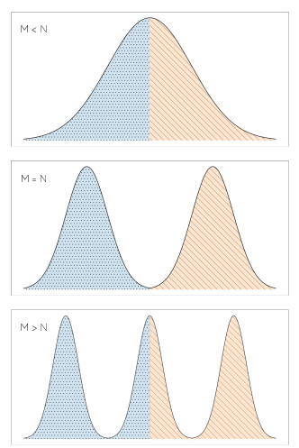
Figure 1: Illustration of the expected behaviour DoPaNet using two discriminators ($N=2$), in case of a Uni-modal ($M=1$, top), bi-modal ($M=2$, middle) and tri-modal ($M=3$, bottom) target distribution. The classifier ensures that the generated modes (in orange and blue) corresponding to two different discriminators do not overlap.

1 Introduction

Generative Adversarial Networks (Goodfellow et al., 2014a) (GANs) consist of a deep generative model which is trained through a minimax game involving a competing generator and discriminator. The discriminator is tasked to differentiate real from fake samples, whereas the generator strives to maximize the mistakes of the discriminator. At convergence, the generator can sample from an estimate of the underlying real data distribution. The generated images, are observed to be of higher quality than models trained using maximum likelihood optimization. Consequently, GANs have demonstrated impressive results in various domains such as image generation (Gulrajani et al., 2017), video generation (Vondrick et al., 2016), super-resolution (Ledig et al., 2017), semi-supervised learning (Donahue et al., 2017) and domain adaptation (Zhu et al., 2017).

GANs are trained with the objective of reaching a Nash-equilibrium (Mescheder, 2018), which refers to the state where neither the discriminator nor the generator can further enhance their utilities unilaterally. However, the generator might miss some modes of the distribution even after reaching the equilibrium as it can simply fool the discriminator by generating from only few modes of the real distribution (Goodfellow, 2016; Arjovsky & Bottou, 2017; Che et al., 2017; Chen et al., 2016; Salimans et al., 2016), and hence producing a limited diversity in samples. To address this problem, the literature explores two main approaches: Improving GAN learning to practically reach a better optimum (Arjovsky & Bottou, 2017; Metz et al., 2017; Salimans et al., 2016; Arjovsky et al., 2017; Gulrajani et al., 2017; Berthelot et al., 2017), or explicitly forcing GANs to produce various modes by design (Chen et al., 2016; Ghosh et al., 2017; Durugkar et al., 2017; Che et al., 2017; Liu & Tuzel, 2016). We hereby follow the latter strategy and propose a new way of dealing with GAN mode collapse. By noticing that using a single discriminator often leads to the generator covering only a part of the data, we bring more discriminators to the game such that each incentivises the generator to cover an additional mode of the data distribution. For each discriminator to focus on a different target mode, we introduce a third player, a classifier $Q$ that decides the discriminator to be trained using a given real sample. To ensure that these various target data modes do not collapse into the same mode, the classifier $Q$ also decides the discriminator to train the generator for a given generated sample. We find that this strategy, illustrated in Figure 2, yields better coverage of the real data distribution at convergence and simultaneously improves the stability of the training as well.

We showcase our method on demonstrative toy problems and show that it outperforms competing methods in avoiding mode collapse. We show that the $Q$ network is able to distinguish different modes of the real data and therefore each discriminator works on a separate mode. This ensures that the generator can sample from a different mode for every input code vector. We also show DoPaNet’s ability to generate good quality and diversified images covering various modes present in the datasets of real images.

We also provide theoretical analysis to show that at global optimum of the objective, the generator replicates the real distribution, categorized into different modes such that it can sample from any mode given the corresponding code vector $c$.

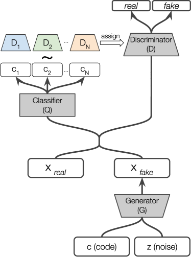
Figure 2: DoPaNet, our proposed framework. Here $\sim$ denotes a sampling operation from the categorical probability distribution $Q(x)$. $c$ is a categorical code with one-hot encoding. Using the resulting category index $\sigma\sim Q(x)$ we select the corresponding discriminator $D_{i=\sigma}$ and connect it to the computation graph. From the perspective of the real sample $x$ and the generated sample $\hat{x}$ the respective computation graph is fully-differentiable, and can be trained like the standard GAN (Goodfellow et al., 2014b).

2 Related work

There is a rich literature on improving training stability and increasing sample diversity for GANs. We only focus on a selection of works that relate closely to ours. (Arora et al., 2017b) introduces theoretical formulation stating the importance of multiple generators and discriminators in order to completely model the data distribution. GMAN (Durugkar et al., 2017) proposes using multiple discriminators. They explore 3 settings where the generator can either be trained against the best discriminator, the averaged discriminators, or the weighted averaged discriminators. This helps training the network without modifying the minimax objective. Even though they use multiple discriminators, all of them are trained using all of the available real data, which does not explicitly help in avoiding mode collapse. We improve on this strategy by adding a classifier as a third component, with the task of choosing the discriminator for the given input sample during training, therefore each of the multiple discriminators specializes on a different part of the real data distribution. We also compare DoPaNet with GMAN (Durugkar et al., 2017) in our experiments (Section 4). Triple-GAN (Li et al., 2017) incorporates a classifier in the adversarial training but it focuses on semi-supervised learning and therefore it needs some part of the real data to be labeled during training. It uses only one discriminator which is also conditioned on the sample labels. Contrarily our aim is to circumvent the mode collapse problem in the general case where the labels of the samples may not be available. InfoGAN (Chen et al., 2016) uses a $Q$ network to maximize mutual information between the input code to the generator and its generated samples. It helps in disentangling several factors of variation, e.g. writing styles in case of digits, pose from lightning, etc. It is different from our approach as it uses the $Q$ network as well to train the generator. Hence it is possible that the generator colludes with $Q$ in disentangling the factors of variation, but simultaneously fooling the discriminator, while sampling from only few modes of the data. It can therefore still face the mode collapse problem which we show in the experiments (Section 4). Several works propose using multiple generators (Arora et al., 2017a; Ghosh et al., 2016; Liu & Tuzel, 2016). For instance, MAD-GAN (Ghosh et al., 2017) improves the learning by compelling the generators to produce diverse modes implicitly using the discriminator. This is achieved by requiring the discriminator to identify the generator that produced the fake samples along with recognizing fake samples from reals. The discriminator does not explicitly force each generator to capture a different mode, while in our case the generator is urged to capture distinct modes by being trained with different discriminators. We also show DoPaNet’s superiority over MAD-GAN in our experiments (Section 4).

3 Method

In this section we first briefly discuss the preliminaries (3.1): the general objective for training Generative Adversarial Nets and conditional sampling and training. Then we detail the objective of DoPaNet (3.2) and how we optimize it.

3.1 Preliminaries

Generative Adversarial Networks

Generative adversarial networks can be considered as a game, where players in the form of neural networks are optimized against each other. Let $p_{d}$ be the $real$ data distribution and $p_{g}$ be the distribution learnt by the generator $G$. Different tasks are assigned to the players: firstly, the generator $G$ takes an input noise $z\sim p(z)$ and returns a sample $\hat{x}=G(z)$. The discriminator $D$ takes an input $x$ which can either be a real sample from the training set or a sample produced by the generator. The discriminator then outputs a conditional probability distribution over the source of the sample $x$. In practice $D$ is a binary classifier that ideally outputs $1$ if the sample is real and $0$ if the sample is fake. Formally the following min-max objective is iteratively optimized:

$$\begin{split}\mathop{\min}_{G}\mathop{\max}_{D}V(D,G):=&\mathop{\mathbb{E}}_{x\sim p_{d}}\left[\log D\left(x\right)\right]\\ &+\mathop{\mathbb{E}}_{z\sim p_{z}}\left[\log\left(1-D\left(G\left({z}\right)\right)\right)\right]\end{split}$$ (1)

The parameters of D are updated to maximize the objective while the generator $G$ is trained to minimize it.

Conditional generation

We can condition the modeled distribution by making $G$ take a code vector $c$ as an additional input to produce a sample $\hat{x}_{c}=G(z,c)$, as it is done in InfoGAN (Chen et al., 2016) and other conditional variants (Mirza & Osindero, 2014). In our case, we restrict the code vector $c$ to have a one-hot encoding. Defining the conditional probability distribution as $Q(x)=p_{c\mid x}$, we obtain an objective function for the classifier $Q$, the general cross-entropy loss:

$$\mathop{\min}_{Q}L(Q,G):=\mathop{\mathbb{E}}_{z\sim p_{z},c\sim p_{c}}\left[CE(c,Q\left(G\left(z,c)\right)\right)\right]$$ (2)

where $CE(.,.)$ is the cross entropy function. The conditional variants of the standard GAN settings optimize both Objectives (1) and (2), where $G$ may or may not be optimized over Objective (2). We do not use $G$ to optimize the Objective (2).

Algorithm 1 DoPaNet training algorithm

1:  for number of training iterations do

2:     Sample minibatch of $m$ noise samples $\{{z}^{(1)},\dots,{z}^{(m)}\}$ from the noise prior $p_{z}({z})$.

3:     Sample minibatch of $m$ code samples $\{{c}^{(1)},\dots,{c}^{(m)}\}$ from the code prior $p_{c}({c})$.

4:     Sample minibatch of $m$ examples $\{{x}^{(1)},\dots,{x}^{(m)}\}$ from the data generating distribution $p_{d}({x})$.

5:     Update $Q$ by ascending its stochastic gradient:

$$\nabla_{\theta_{q}}\frac{1}{m}\sum_{i=1}^{m}c^{(i)}\cdot\log Q\left(G\left(z^{(i)},c^{(i)}\right)\right)$$

6:     Decide for every input which of the $N$ discriminators to use by sampling from the likelihood distribution of $Q$:

$$\sigma(i)\sim Q\left(x^{(i)}\right)\qquad\hat{\sigma}(i)\sim Q\left(G\left(z^{(i)},c^{(i)}\right)\right)$$

7:     $\forall n\in[1,\dots,N]$, define the set of samples that are assigned to the $n^{\text{th}}$ discriminator $D_{n}$ as:

$$\mathcal{D}_{n}=\left\{x^{(i)}|\sigma(i)=n\right\}\qquad\hat{\mathcal{D}}_{n}=\left\{G\left(z^{(i)},c^{(i)}\right)\rvert\hat{\sigma}(i)=n\right\}$$

8:     $\forall n\in[1,\dots,N]$, update the $n^{\text{th}}$ discriminator by ascending its stochastic gradient:

$$\nabla_{\theta_{d_{n}}}\left(\frac{1}{|\mathcal{D}_{n}|}\sum_{x\in\mathcal{D}_{n}}\log D_{n}\left(x\right)+\frac{1}{|\hat{\mathcal{D}}_{n}|}\sum_{\hat{x}\in\hat{\mathcal{D}}_{n}}\log\left(1-D_{n}\left(\hat{x}\right)\right)\right)$$

9:     Sample minibatch of $m$ noise samples $\{{z}^{(1)},\dots,{z}^{(m)}\}$ from the noise prior $p_{z}({z})$.

10:     Sample minibatch of $m$ code samples $\{{c}^{(1)},\dots,{c}^{(m)}\}$ from the code prior $p_{c}({c})$.

11:     Decide for every $i^{\text{th}}$ input which of the $N$ discriminators to use by sampling from likelihood distribution of $Q$:

$$\hat{\sigma}(i)\sim Q\left(G\left(z^{(i)},c^{(i)}\right)\right)$$

12:     Update the generator by descending its stochastic gradient:

$$\nabla_{\theta_{g}}\frac{1}{m}\sum_{i=1}^{m}\log\left(1-D_{\hat{\sigma}(i)}\left(G\left({z}^{(i)},{c}^{(i)}\right)\right)\right)$$

13:  end for

3.2 Our approach: DoPaNet

DoPaNet consists of three main components: A conditional generator $G$, a classifier $Q$ and a set of independent discriminators $\{D_{i}\}$. We use categorical code vectors $c\in\{0,1\}^{N}$ with one-hot encoding where $N$ is the number of discriminators used. We use the notation $c_{i}$ to denote the one-hot code vector $c$ with value at the $i^{\text{th}}$ index as 1. As illustrated in Figure 2, $G$ generates a sample $\hat{x}_{c}=G(z,c)$. Next we feed the sample to the classifier Q to get the categorical probability distribution. For each generated sample we draw $\hat{\sigma}\sim Q(\hat{x}_{c})$, i.e. $\hat{\sigma}\in[1,...,N]$ that decides the corresponding discriminator and $D_{\hat{\sigma}}$ that is going to process the generated sample. Formally, we define $D(\hat{x}):=D_{\hat{\sigma}}(\hat{x}_{c})$. Similarly, for the real sample $x\sim p_{d}$, we draw $\sigma\sim Q(x)$ and define the discriminator $D(x):=D_{\sigma}(x)$ for the sample $x$. Thus, for every sample, the discriminator used is decided by the classifier $Q$. This yields a fully-differentiable computational graph, despite the fact that the sampling operation $\sigma\sim Q(x)$ is non-differentiable. In other words, once $D$ is selected using predictions from $Q$, the training requires no further modifications to the standard GAN optimization algorithm, therefore it is compatible with all recent advanced variants of GANs. In our experiments we define $p_{z}$ as a standard normal distribution and $p_{c}$ as a uniform categorical distribution unless otherwise stated.

Let us define the minimax objective for DoPaNet:

$$\begin{split}\mathop{\min}_{G}\mathop{\max}_{\{D_{i}\}_{i=1}^{N}}&M(\{D_{i}\}_{i=1}^{N},G):=\mathop{\mathbb{E}}_{\begin{subarray}{c}x\sim p_{d}\\ \sigma\sim Q(x)\end{subarray}}\left[\log D_{\sigma}\left({x}\right)\right]\\ &+\mathop{\mathbb{E}}_{\begin{subarray}{c}z\sim p_{z},c\sim p_{c}\\ \hat{\sigma}\sim Q(G(z,c))\end{subarray}}\left[\log\left(1-D_{\hat{\sigma}}\left(G\left({z},{c}\right)\right)\right)\right]\\ \end{split}$$ (3)

We train DoPaNet by iteratively optimizing the following objective function (refer Algorithm 1):

$$\mathop{\min}_{G}\mathop{\max}_{\{D_{i}\}_{i=1}^{N}}M(\{D_{i}\}_{i=1}^{N},G)+\mathop{\min}_{Q}L(Q,G)$$ (4)

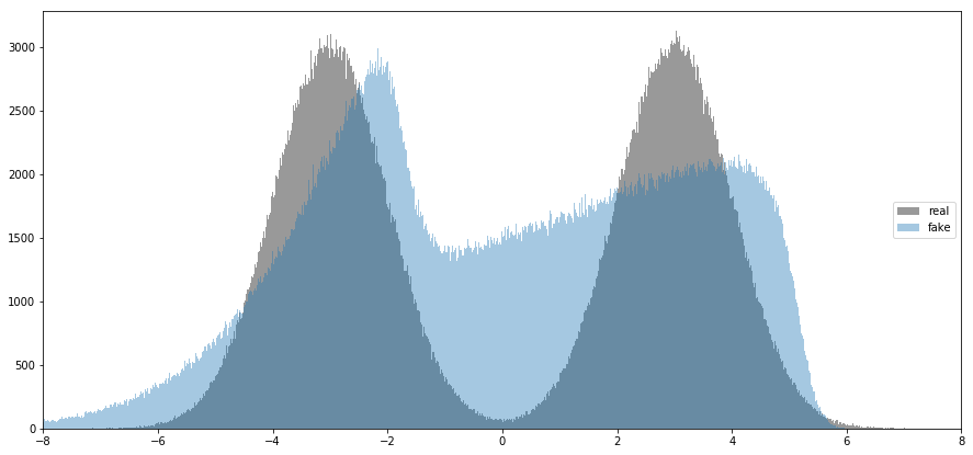
(a) Standard GAN

(b) DoPaNet, 2 modes, 2 Disc.

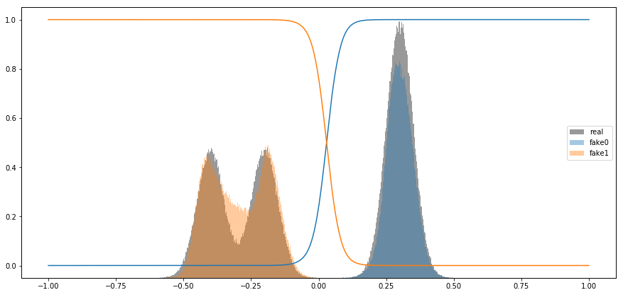
(c) DoPaNet, 3 modes, 2 Disc.

Figure 3: Theoretical analysis: The figures are plotted using 100000 samples and 1000 bins histogram where the grey area represents the real data distribution. Fig. (a): Standard GAN - In special case, $N=1$ DoPaNet is equivalent to the standard GAN. The blue area represents the model distribution. Fig. (b, c): The orange and blue area represent the generations corresponding to $c_{1}$ and $c_{2}$. The number of discriminators is fixed at $N=2$, while the number of modes is $M=2,3$ respectively. The orange and blue curves depict the predicted class probability of $c_{1}$ and $c_{2}$ respectively by the classifier $Q$. It can be seen that support of $p_{d}^{1}$ (i.e. $x<0$) can be considered disjoint from the support of $p_{d}^{2}$ (i.e. $x>0$) due to steep change in $p_{c\mid x}$ around $x=0$. It also shows that the real distribution area corresponding to $c_{1}$ and $c_{2}$: $\rho_{S_{1}}$ and $\rho_{S_{2}}$ is almost equal in proportion and therefore equal to 1/2.

3.3 Theoretical Analysis

The classifier $Q$ is trained only using Objective 2, and is applied on the generated samples $\hat{x}$ as well as the real samples $x$ to decide the discriminator to use. It is optimal when it is able to correctly classify the generated samples $\hat{x}$ into their corresponding $c_{i}$’s. Empirically we observe that the classifier $Q$ is easily able to reach its optimum, as can be observed in the Figure 3(b) and 3(c), as the blue and orange curves (samples predicted as $c_{1}$ and $c_{2}$ respectively) coincide with the samples forming blue and green area (samples generated using $c_{1}$ and $c_{2}$ respectively). Interestingly, we observe that the classifier $Q$ is able to indirectly control the generator $G$ through the discriminators as $G$ groups its generations according to the code vectors $c_{i}$.

Here we provide formal theoretical formulation of our model with proof presented in Appendix A.

Lemma 3.1.

For optimal $Q$ and fixed $G$, the optimal $D_{i}$, $\forall i\in[1,\dots,N]$ is

$$D^{*}_{i}(x)=\frac{\rho_{S_{i}}p_{d}^{i}(x)}{\rho_{S_{i}}p_{d}^{i}(x)+\frac{1}{N}p_{g}^{i}(x)}$$ (5)

where $S_{i}=\{x\in Supp(p_{d})|Q(x)=c_{i}\}$, $\rho_{S_{i}}=\int_{x\in S_{i}}p_{d}(x)\mathrm{d}x$, $p_{d}^{i}$ is a probability distribution such that $p_{d}^{i}(x)=\frac{p_{d}(x)}{\rho_{S_{i}}}$ and $Supp(p_{d}^{i})=S_{i}$, and $p_{g}^{i}(x)=p_{z}(z)$ such that $G(z,c_{i})=x$.

We can now reformulate the minimax game as

$$U(G)=\mathop{\max}_{\{D_{i}\}_{i=1}^{N}}M(\{D_{i}\}_{i=1}^{N},G)$$

Theorem 3.2.

In case of $N$ discriminators, the global minimum of $U(G)$ is achieved if and only if $p_{g}^{i}(x)=p_{d}^{i}(x)$, $\forall i\in[1,\dots,N]$. When $\rho_{S_{i}}=1/N$, the global minimum value of $U(G)$ is $-\log(4)$.

Sampling from $p_{d}^{i}$ is same as sampling from the $i^{\text{th}}$ mode of the real distribution, the mode that covers the set of samples $S_{i}=\{x\in Supp(p_{d})|Q(x)=c_{i}\}$. Please note that we can assume that each of $\{p_{d}^{i}\}_{i=1}^{N}$ has a disjoint support. Figure 3(b) and 3(c) empirically show that the assumption of disjoint support of the distributions $p_{d}^{1}$ and $p_{d}^{2}$, which is decided by the classifier $Q$, is valid.

So, in theory each $G_{i}(.)=G(.,c_{i})$ should converge to a different mode as the target dataset distribution $p_{d}^{i}$ is itself different $\forall i\in[1,\dots,N]$. Hence, empirically the number of modes covered should essentially be at least more diverse than the standard GAN model. This is also observed in all our experiments as well as when comparing the Figures  3(a) and 3(b).

Corollary 3.2.1.

At global minimum of $U(G)$, the generative model $G$ replicates the real distribution $p_{d}$, categorized into different modes.

Thus our model DoPaNet can learn the real data distribution while also controlling the diversity of the generations by sampling from a different real mode corresponding to each $c_{i}$, which we also verify experimentally in the next section.

4 Experiments

We demonstrate the performance of our method DoPaNet on a diverse set of tasks with increasing complexity, involving probability density estimation and image generation. To illustrate the functioning of DoPaNet, we first set up two low-dimensional experiments (Section 4.1) using Gaussian Mixture Models (GMMs) as the target probability density function: 1D GMM and 2D GMM. For the 1D Gaussian Mixture case, we compare DoPaNet’s robustness against other approaches by reproducing the experiment setting detailed in (Ghosh et al., 2017) and we outperform all competing methods both qualitatively and quantitatively. We also show DoPaNet’s performance using multiple discriminators and show how the training dynamics change according to the number of discriminators. We observe that increasing the number of discriminators improves the performance of the network until the point where the number of discriminators exceeds the number of underlying modes. Using the 2D circular GMM, we show that classifier $Q$ is able to learn good partitioning of the distribution and therefore each discriminator acts on samples from a different mode unlike GMAN (Durugkar et al., 2017). We show that DoPaNet is able to utilize the capacity of multiple discriminators and we can control the mode the generator samples from using the code $c$. Even in this case, DoPaNet performs better in capturing all the modes.

We finally demonstrate qualitative results on commonly investigated datasets: Stacked-MNIST, CIFAR-10 and CelebA in Section 4.2. DoPaNet is able to generate good quality diverse samples. In case of CIFAR-10, we also show that we can generate samples from every class given the class label $y$. The information about the network architectures and the implementation details are provided in Appendix D.

4.1 Synthetic low dimensional distributions

In DoPaNet, the role of the classifier $Q$ is to partition both the real and generated data-points into different clusters or modes, and each discriminator is consequently only trained on a separate cluster. In order to fully understand how this helps the training, we experimented with two toy datasets obtained using mixture of Gaussian variants: a 1D GMM with 5 modes, as used in (Ghosh et al., 2017), and a 2D circular GMM with 3 and 8 modes on the unit circle.

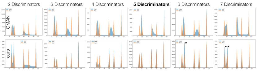
Figure 4: To study the behaviour of multi-discriminator settings with different number ($N$) of discriminators, we trained GMAN (Durugkar et al., 2017) and DoPaNet on a 1D data set with 5 modes. Both GMAN’s (top) and DoPaNet’s (bottom) results improved by adding discriminators while $N$ is less or equal the number of modes. To justify this, we point at the case where $N=5$: the models perform best since each class has to capture only a single mode. In the case of $N=6$ and $N=7$ DoPaNet decreased in performance only due to oversampling (marked with $*$ and $**$) of some classes.

4.1.1 Experiment setup and Evaluation details

First, we reproduced the 1D setting in (Ghosh et al., 2017) with 5 modes at $[10,20,60,80,110]$ and standard deviations $[3,3,2,2,1]$ respectively and we compare to the numbers reported in that paper in Table 1. We sampled $65,536$ data points each from the real distribution and the generator distribution. For each of these two distributions, we created a histogram using bin size of $0.1$ with bins lying in the range of $-10$ to $130$. We then obtained Chi-square distance as well as KL divergence between the generator distribution and the true data distribution using these two histograms. To compare against GMAN using different number of discriminators, we used $1,000,000$ samples (instead of $65,536$ above) and show the results in Table 2 and Figure 4.

We then introduce a 2D experiment setting with 2D Gaussian Mixture Model (GMM). It has multiple modes having covariance matrix of $0.01I$, where $I$ is an identity matrix, and equally separated means lying on a unit circle (please refer to Figure 5 for the $3$ mode case). For Table 3 we consider $8$ modes and construct histograms using $1,000,000$ samples and bin size of $0.0028\times 0.0028$ with bins lying in the range of $[-1.4,1.4]\times[-1.4,1.4]$.

For these experiments, we use uniform distribution $U(-1,1)$ of dimension $64$ for $p_{z}$ and uniform categorical distribution for $p_{c}$ to get the generations in both 1D and 2D experiments.

GAN Variants	Chi-square($\times 10^{5}$)	KL-Div
DCGAN∗	0.90	0.322
WGAN∗	1.32	0.614
BEGAN∗	1.06	0.944
GoGAN∗	2.52	0.652
Unrolled GAN∗	3.98	1.321
Mode-Reg DCGAN∗	1.02	0.927
InfoGAN∗	0.83	0.210
MA-GAN∗	1.39	0.526
MAD-GAN∗	0.24	0.145
GMAN	1.44	0.69
DoPaNet	0.03	0.02

Table 1: 1D Gaussian Mixture Model experiment using best results from 3 runs for GAN variants that aims to solve mode collapse. Results for the GAN variants marked as $*$ were reproduced from (Ghosh et al., 2017).

4.1.2 Observations

Comparing against other GAN variants

In Table 1, we show that DoPaNet outperforms other GAN architectures on the 1D task by a large margin in terms of Chi-square distance and KL-Divergence. We believe that the success is due to the classifier $Q$’s capability to learn to partition the underlying distribution easily. We also show in Table 3, that in the 2D task DoPaNet achieves better performance than GMAN (Durugkar et al., 2017) in terms of both KL-Divergence an Chi-square.

Benchmarking the number of discriminators

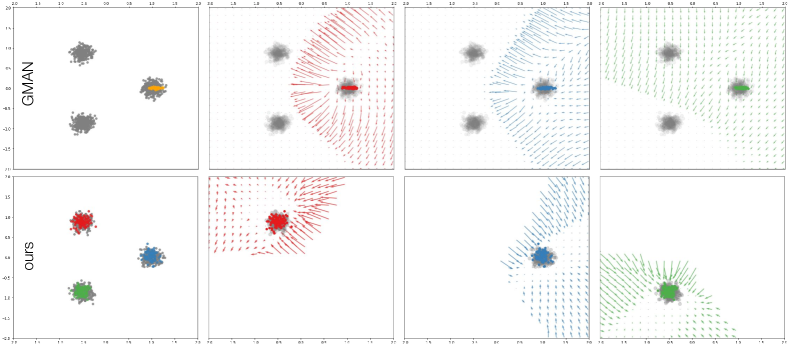
Figure 5: A circular 2D GMM with 3 modes on the unit circle with standard deviations of 0.01. We train GMAN and DoPaNet with $N=3$ setting. In the first column we show the generated distribution for each method in colours (orange for GMAN, a single color since GMAN uses no conditioning on their samples, and red, green and blue in DoPaNet’s case for samples generated using $c_{1}$, $c_{2}$ and $c_{3}$ respectively). In columns 2, 3 and 4 we plotted the gradient field for each of the equally separated data-points present in $[-2.0,2.0]\times[-2.0,2.0]$. Different colors show the gradient by different discriminators. For GMAN, each column shows the gradient field by the respective discriminator for each of the data-points. For DoPaNet, each of the data-points is first classified by $Q$ and the respective discriminator is used to get the gradient field, which is shown in the corresponding column of 2-3. We see how classifier $Q$ indirectly pushes different modes generated by $G$ apart, more importantly the gradient field has the highest magnitude in the direction which separates the modes, while this phenomenon is not happening in the case of GMAN.

$N$	Chi-square($\times 10^{7}$)		KL-Div
	GMAN	DoPaNet	GMAN	DoPaNet
2	5.00$\pm$6.80	1.89$\pm$0.92	1.74$\pm$0.63	0.81$\pm$0.27
3	2.96$\pm$2.88	1.10$\pm$2.43	1.50$\pm$0.57	0.55$\pm$0.36
4	3.41$\pm$2.73	0.74$\pm$0.98	1.48$\pm$0.42	0.50$\pm$0.41
5	4.62$\pm$3.92	0.27$\pm$0.54	1.55$\pm$0.30	0.25$\pm$0.26
6	3.94$\pm$3.22	0.41$\pm$0.50	1.56$\pm$0.22	0.35$\pm$0.20
7	2.84$\pm$1.51	0.42$\pm$0.43	1.45$\pm$0.38	0.36$\pm$0.21
8	2.80$\pm$1.55	0.93$\pm$1.14	1.36$\pm$0.43	0.56$\pm$0.31

Table 2: 1D Gaussian Mixture Model experiment using best results from 20 runs with different number of discriminators ($N$) as illustrated in Figure 4.

We study the change in performance with regards to the number of discriminators used by both GMAN (Durugkar et al., 2017) and DoPaNet. The clustering mechanism with varying number of discriminators is illustrated on the 1D task in Figure 4. We see in this experiment that classes of the generated samples are first attracted towards larger clusters of the real data. By adding more discriminators, the quality of the reconstructed modes is refined. The refinement process starts first with the easiest separation, between the $2^{nd}$ and the $3^{rd}$ peaks, after that the $4^{th}$ and $5^{th}$ modes are distinguished by the classifier $Q$, and so on. We quantitatively see in Table 2 that increasing the number of discriminators improves the performance of both GMAN and DoPaNet up to a certain point where $N$ (number of discriminators) matches the number of modes in the data. After this optimal point, increasing $N$ yields a decreasing performance, because already captured modes are oversampled. In Figure 4 we have marked examples of oversampling in the last two columns with $*$ symbols.

GAN Variants	Chi-square($\times 10^{6}$)	KL-Div
Standard GAN	3.883	2.860
GMAN	1.253	0.636
DoPaNet	0.449	0.246

Table 3: 2D Gaussian Mixture Model experiment with $M=N=8$ (where $N$ is the number of discriminators, $M$ is the number of Gaussians used in the mixture model). For each experiment, we use a fixed set of 1,000,000 samples and do 5 runs for each algorithm and report the results using the best run. We took effort to make sure that the comparison was fair, and used the same set of parameters as in the 1D experiments.

It is interesting to note that when the same experiment was carried out in MADGAN (Ghosh et al., 2017), which uses multiple generators, their performance peaked at $N_{Generators}=4$ unlike GMAN and ours, both of which logically peaked at $N_{Discriminator}=5$ considering that there are $5$ visible modes. This shows a difficulty in tuning the hyper-parameter $N_{Generators}$ in (Ghosh et al., 2017) for different applications.

2D experiments

In 2D experiments, for both GMAN (Durugkar et al., 2017) and DoPaNet we experiment with $N=M=8$ (where $N$ is the number of discriminators, $M$ is the number of modes) for both quantitative (listed in Table 3) and qualitative results (see Appendix B), and the $N=M=3$ setting for qualitative results (illustrated in Figure 5). In all of the runs, DoPaNet was able to capture, and classify all modes of the true distribution correctly, while GMAN (Durugkar et al., 2017) failed on both the $N=M=3$ as well as the $N=M=8$ setting.

In Figure  5 we show a circular 2D GMM with 3 modes on the unit circle which is used to train GMAN and DoPaNets. In the case of DoPaNet, it can also be observed (see column 1) that the generator generates from a different mode for a different $c_{i}$. We can also visually see that the classifier $Q$ is indirectly able to control the conditioned samples $G(z,c)$ by routing them to the corresponding discriminators (see columns 2-3). It also illustrates that we are indeed able to utilize the capabilities of multiple $D_{i}$’s as intended: different discriminators begin to specialize on different modes and therefore provide different gradients for the respective mode as well. Although being trained with the generated code vectors only, DoPaNet’s classifier $Q$ achieves fine partitioning of the original distribution. We suggest that our approach succeeds because each discriminator is fed different samples from the beginning. $Q$ is initialized to assign each real sample to every discriminator with equal probability, but given that the generator samples different points for every code vector $Q$ quickly learns the different modes that the samples from $G_{i}$ are attracted towards (where $G_{i}$ refers to the conditional distribution modeled by $G(z,c_{i})$). Given that the updated $Q$ is already providing different subsets of the input space to the different discriminators, the discriminators will provide different gradients for each corresponding code vector. Therefore $G$ learns to separate the modes of the learnt distributions conditioned on $c$ from each other. We argue that GMAN is not able to utilize multiple discriminators in this experiment setup and that most of the learning is done by just a few discriminators rather than their effective ensemble (see Appendix B).

4.2 Image generation

After investigating the DoPaNet performance on low dimensional tasks, now we validate DoPaNet on real image generation tasks.

4.2.1 Stacked-MNIST

We first investigate how well DoPaNet can reconstruct the real distribution of the data using the Stacked-MNIST dataset (Srivastava et al., 2017). This dataset contains three channel color images, containing a randomly selected sample from the MNIST dataset in each channel. This results in ten possible modes on each channel so the number of all the possible modes in the dataset is $10^{3}$. It was shown in (Ghosh et al., 2017) that various architectures recovered only a small portion of these modes. A qualitative image depicting the recovered modes using the traditional DCGAN (Radford et al., 2016) architecture and DoPaNet can be seen in Figure 2. We have also measured the Kullback-Leibler divergence between the real distribution and the generated distributions. We compare DoPaNet against the other GAN variants in Table 4.

GAN Variants	KL Div
DCGAN∗ (Radford et al., 2016)	2.15
WGAN∗ (Arjovsky et al., 2017)	1.02
BEGAN∗ (Berthelot et al., 2017)	1.89
GoGAN∗ (Juefei-Xu et al., 2017)	2.89
Unrolled GAN∗ (Metz et al., 2017)	1.29
Mode-Reg DCGAN∗ (Che et al., 2017)	1.79
InfoGAN∗ (Chen et al., 2016)	2.75
MA-GAN∗ (Ghosh et al., 2017)	$3.4$
MAD-GAN∗ (Ghosh et al., 2017)	0.91
GMAN (Durugkar et al., 2017)	2.17
DoPaNet (ours)	0.13

Table 4: Stacked-MNIST: we compare our method against several GAN variants. Through this experiment using a real dataset, we can show that DoPaNet is closer to the real distribution. Results for the GAN variants marked as $*$ were reproduced from (Ghosh et al., 2017).

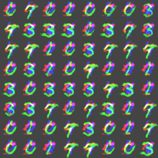
(a)

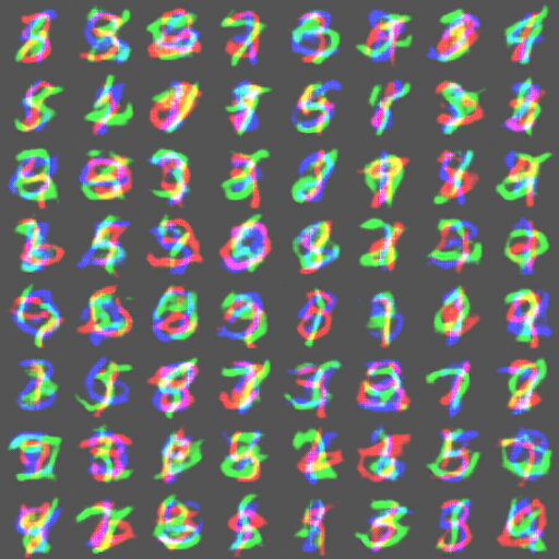
(b)

Figure 6: Sample images from stacked mnist. The samples on the left (a) were generated using the traditional architecture of DCGANwhile the samples on the right (b) were generated using DoPaNet with $10$ discriminators ($N=10$). Visually, (a) appears to be more clear as only one color (green) is dominating over digits of the other two colors while in (b) more digits are covered per sample which refers to higher diversity in the modeled distribution, thus better mode coverage.

4.2.2 Qualitative results on CIFAR-10 and celebA

To show the image generation capabilities of DoPaNet, we trained the multi discriminator setting on a lower and a higher complexity image generation task, CIFAR-10 and CelebA respectively. We compare our results qualitatively to the ones reported by GMAN (Durugkar et al., 2017) on both tasks in Figure 9.

CIFAR-10

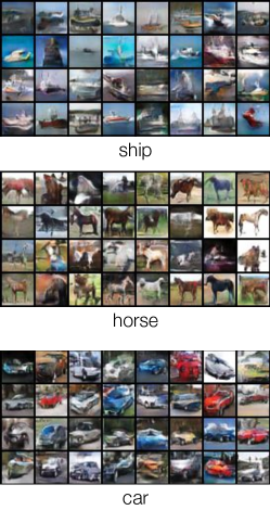
Figure 7: $32\times 32$ CIFAR-10 samples drawn from DoPaNet trained with $N=5$ discriminators for 700k iterations. The generations in each subfigure correspond to $y=1,2$ and $3$ respectively. We call the attention to the various different details learnt for each class which can cause mode collapse in other GAN variants.

While learning the distribution of $32\times 32$ colored images may sound easy, the main challenge is to learn geometric structures from low resolution and reproduce them in various colors, backgrounds, angles etc. Following (Mescheder et al., 2018), the generator takes ground truth label $y$ as input as well along with the code $c$, and the discriminator outputs a $10$ dimensional output of which only the $y^{\text{th}}$ index is used for training $D_{\sigma}$ as well as $G$, while $Q$ is trained just using the code $c$. Thus, the code $c$ helps it learn class invariant features. We illustrate in Figure 7 that DoPaNet is capable of capturing these features such as different object orientations and colors depicted in various weather conditions. It is also able to recognize minute details like wheels, horse hair, ship textures, etc. We present more generations corresponding to each of the classes in Appendix C.

CelebA

We also show DoPaNet performance on large scale images such as $128\times 128$ by training a residual network for 100k iterations on the celebA dataset. This dataset contains various modes like lighting, pose, gender, hair style, clothing, facial expressions which are challenging to capture for generative models. In Figure 8 we demonstrate that DoPaNet is capable of recovering the aforementioned visual features.

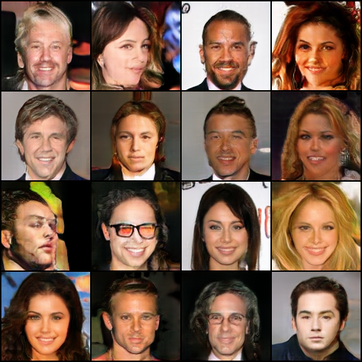
Figure 8: Random samples from DoPaNet trained at scale of $128\times 128$ images on unaligned CelebA set for 100k iterations. As it can be seen, different faces appear in diverse poses with different background, and rarely occurring accessories such as orange sunglasses are learned by the model.

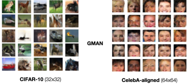
Figure 9: Random samples presented in (Durugkar et al., 2017) for image generation tasks such as CIFAR-10 and CelebA. Best results were achieved with GMAN-0 variant with $N=5$ discriminators. For CelebA they cropped the images to exclude background.

5 Discussion

We conclude that it is not necessary for a generator to have equal capacity adversary to converge, meaning that the standard GAN training procedure could be enhanced with multiple (and even weaker) discriminators specialized only in attracting the model distribution of the generator to their corresponding modes.

DoPaNet is proven experimentally to utilize the capability of multiple discriminators by partitioning the target distributions into several identifiable modes and making each discriminator work on a separate mode. Thus, it reduces the complexity of the modes to be learnt by each discriminator. We show qualitatively and quantitatively that DoPaNet is able to better cover the real distribution. We observe that the generator is also able to sample from different identifiable modes of the data distribution given the corresponding code vectors.

Appendix

Here we first give the theoretical formulation of our work DoPaNet to show that the modes captured should be different for each categorical code $c_{i}$ and that the standard GAN can be considered as its lower bound on mode collapse. We then give some more experimental insights from the 2D task. We also give some more generations using CIFAR. Later we provide implementation details of the network architectures we used.

Appendix A Theoretical formulation

Here we present the theoretical formulation for our proposed method DoPaNet.

Lemma 3.1.

For optimal $Q$ and fixed $G$, the optimal $D_{i}$, $\forall i\in[1,\dots,N]$ is

$$D^{*}_{i}(x)=\frac{\rho_{S_{i}}p_{d}^{i}(x)}{\rho_{S_{i}}p_{d}^{i}(x)+\frac{1}{N}p_{g}^{i}(x)}$$ (6)

where $S_{i}=\{x\in Supp(p_{d})|Q(x)=c_{i}\}$, $\rho_{S_{i}}=\int_{x\in S_{i}}p_{d}(x)\mathrm{d}x$, $p_{d}^{i}$ is a probability distribution such that $p_{d}^{i}(x)=\frac{p_{d}(x)}{\rho_{S_{i}}}$ and $Supp(p_{d}^{i})=S_{i}$, and $p_{g}^{i}(x)=p_{z}(z)$ such that $G(z,c_{i})=x$.

Proof.

Let us consider a case where we have $N=2$ discriminators. The theoretical formulation for this case can be trivially extended to more number of discriminators. The objective being optimized by the generator and the discriminators is (Obj. 3):

$$\begin{split}\mathop{\min}_{G}\mathop{\max}_{D_{1},D_{2}}&M(\{D_{1},D_{2}\},G):=\Bigg{[}\mathop{\mathbb{E}}_{\begin{subarray}{c}x\sim p_{d}\\ \sigma\sim Q(x)\end{subarray}}\left[\log D_{\sigma}\left(x\right)\right]\\ +&\mathop{\mathbb{E}}_{\begin{subarray}{c}z\sim p_{z},c\sim p_{c}\\ \hat{\sigma}\sim Q(G(z,c))\end{subarray}}\left[\log\left(1-D_{\hat{\sigma}}\left(G\left({z},{c}\right)\right)\right)\right]\Bigg{]}\end{split}$$ (7)

When the classifier $Q$ has converged to its optimal form, the above Equation 7 can be rewritten as:

$$\begin{split}\mathop{\min}_{G}\Bigg{[}\mathop{\max}_{D_{1}}\Big{[}&\mathop{\mathbb{E}}_{\begin{subarray}{c}x\sim p_{d}\\ x\in S_{1}\end{subarray}}\left[\log D_{1}\left(x\right)\right]\\ &+p_{c}(c_{1})\mathop{\mathbb{E}}_{z\sim p_{z}}\left[\log\left(1-D_{1}\left(G\left({z,c_{1}}\right)\right)\right)\right]\Big{]}\\ +\mathop{\max}_{D_{2}}\Big{[}&\mathop{\mathbb{E}}_{\begin{subarray}{c}x\sim p_{d}\\ x\in S_{2}\end{subarray}}\left[\log D_{2}\left(x\right)\right]\\ &+p_{c}(c_{2})\mathop{\mathbb{E}}_{z\sim p_{z}}\left[\log\left(1-D_{2}\left(G\left({z,c_{2}}\right)\right)\right)\right]\Big{]}\Bigg{]}\end{split}$$ (8)

where $x\in S_{i}$ if $Q(x)=c_{i}$. $p_{c}$ is the categorical distribution and in our case equal probability is assigned to both the values $c_{1}$ and $c_{2}$. Here $c_{i}$ is that code vector which leads the classifier $Q$ to pass $G\left({z,c_{i}}\right)$ to $D_{i}$ for $i\in[1,2]$. Please note that we can therefore consider $G\left({.,c_{1}}\right)$ as $G_{1}(.)$ and $G\left({.,c_{2}}\right)$ as $G_{2}(.)$, where $G_{1}$ and $G_{2}$ have shared weights except the bias weights in the initial layer. Bias weights in the initial layer are independently trained for $G_{1}$ and $G_{2}$.

The Objective 8 can be rewritten as:

$$\begin{split}\mathop{\min}_{G_{1},G_{2}}\Bigg{[}\mathop{\max}_{D_{1}}\Big{[}&\rho_{S_{1}}\mathop{\mathbb{E}}_{x\sim p_{d}^{1}}\left[\log D_{1}\left(x\right)\right]\\ &+\frac{1}{2}\mathop{\mathbb{E}}_{z\sim p_{z}}\left[\log\left(1-D_{1}\left(G_{1}\left({z}\right)\right)\right)\right]\Big{]}\\ +\mathop{\max}_{D_{2}}\Big{[}&\rho_{S_{2}}\mathop{\mathbb{E}}_{x\sim p_{d}^{2}}\left[\log D_{2}\left(x\right)\right]\\ &+\frac{1}{2}\mathop{\mathbb{E}}_{z\sim p_{z}}\left[\log\left(1-D_{2}\left(G_{2}\left({z}\right)\right)\right)\right]\Big{]}\Bigg{]}\end{split}$$ (9)

where $\rho_{S_{i}}=\int_{x\in S_{i}}p_{d}(x)\mathrm{d}x$. $p_{d}^{i}$ is a probability distribution such that $p_{d}^{i}(x)=\frac{p_{d}(x)}{\rho_{S_{i}}}$ and $Supp(p_{d}^{i})=S_{i}$ where $S_{i}=\{x\in Supp(p_{d})|Q(x)=c_{i}\}$ is the set of samples in the $i^{\text{th}}$ mode of the real distribution. So, sampling from $p_{d}^{i}$ is same as sampling from the $i^{\text{th}}$ mode of the real distribution $p_{d}$. Therefore, $Supp(p_{d})=Supp(p_{d}^{1})\cup Supp(p_{d}^{2})$ and $Supp(p_{d}^{1})\cap Supp(p_{d}^{2})=\emptyset$.

For a fixed generator $G$, $G_{1}$ and $G_{2}$ are also fixed. For a given $G_{1}$ and $G_{2}$, the discriminator $D_{i}$ tries to maximize the quantity (using Objective 9):

$$\begin{split}\rho_{S_{i}}\int_{x}p_{d}^{i}(x)\log D_{i}(x)&\mathrm{d}x\\ +\frac{1}{2}\int_{z}&p_{z}(z)\log(1-D_{i}(G_{i}(z)))\mathrm{d}z\\ =\int_{x}\rho_{S_{i}}p_{d}^{i}(x)\log D_{i}(x)&+\frac{1}{2}p_{g}^{i}(x)\log(1-D_{i}(x))\mathrm{d}x\end{split}$$ (10)

where $p_{g}^{i}(x)=p_{z}(z)$ such that $G_{i}(z)=x$ for $i=1,2$. Therefore, for a fixed generator we get the optimal discriminator $D_{i}$ as:

$$D^{*}_{i}(x)=\frac{\rho_{S_{i}}p_{d}^{i}(x)}{\rho_{S_{i}}p_{d}^{i}(x)+\frac{1}{2}p_{g}^{i}(x)}$$ (11)

In case of $N$ discriminators, the optimal discriminator $D_{i}$ can be similarly obtained as:

$$D^{*}_{i}(x)=\frac{\rho_{S_{i}}p_{d}^{i}(x)}{\rho_{S_{i}}p_{d}^{i}(x)+\frac{1}{N}p_{g}^{i}(x)}$$ (12)

∎

Theorem 3.2.

In case of $N$ discriminators, the global minimum of $U(G)$ is achieved if and only if $p_{g}^{i}(x)=p_{d}^{i}(x)$, $\forall i\in[1,\dots,N]$. When $\rho_{S_{i}}=1/N$, the global minimum value of $U(G)$ is $-\log(4)$.

Proof.

Given the optimal discriminators $D_{1}^{*}$ and $D_{2}^{*}$, we can reformulate the Objective 9 as:

$$\begin{split}\mathop{\min}_{G_{1},G_{2}}\Bigg{[}\rho_{S_{1}}&\mathop{\mathbb{E}}_{x\sim p_{d}^{1}}\left[\log D^{*}_{1}\left(x\right)\right]\\ +&\frac{1}{2}\mathop{\mathbb{E}}_{z\sim p_{z}}\left[\log\left(1-D^{*}_{1}\left(G_{1}\left({z}\right)\right)\right)\right]\\ +\rho_{S_{2}}&\mathop{\mathbb{E}}_{x\sim p_{d}^{2}}\left[\log D^{*}_{2}\left(x\right)\right]\\ +&\frac{1}{2}\mathop{\mathbb{E}}_{z\sim p_{z}}\left[\log\left(1-D^{*}_{2}\left(G_{2}\left({z}\right)\right)\right)\right]\Bigg{]}\end{split}$$ (13)

As noted earlier, bias weights in the initial layer of $G_{1}$ and $G_{2}$ are independently trained with all the other weights shared. As it empirically turns out, the shared weights help learn the similar features, which are essential in low-level image formation and should be similar even if $G_{1}$ and $G_{2}$ were trained independently. So, we can rather relax the restriction and consider $G_{1}$ and $G_{2}$ to be independent of each other. So, the objective 13 can be rewritten as:

$$\mathop{\min}_{G_{1}}W(G_{1})+\mathop{\min}_{G_{2}}W(G_{2})$$ (14)

where,

$$\begin{split}W(G_{i}):=\Bigg{[}\rho_{S_{i}}&\mathop{\mathbb{E}}_{x\sim p_{d}^{i}}\left[\log D^{*}_{i}\left(x\right)\right]\\ +&\frac{1}{2}\mathop{\mathbb{E}}_{z\sim p_{z}}\left[\log\left(1-D^{*}_{i}\left(G_{i}\left({z}\right)\right)\right)\right]\Bigg{]}\end{split}$$ (15)

This is same as optimizing different $G_{i}$-$D_{i}$ pairs on dataset distributions $p_{d}^{i}$ decided by the classifier $Q$ based on the target real distribution $p_{d}$. Figure 3(b) and 3(c) empirically show that the assumption of disjoint support of the distributions $p_{d}^{1}$ and $p_{d}^{2}$ is valid. The Equation 15 can be rewritten as:

$$\begin{split}W(G_{i}):=\Bigg{[}\rho_{S_{i}}&\mathop{\mathbb{E}}_{x\sim p_{d}^{i}}\left[\log D^{*}_{i}\left(x\right)\right]\\ +&\frac{1}{2}\mathop{\mathbb{E}}_{x\sim p_{g}^{i}}\left[\log\left(1-D^{*}_{i}\left(x\right)\right)\right]\Bigg{]}\\ =\Bigg{[}\rho_{S_{i}}&\mathop{\mathbb{E}}_{x\sim p_{d}^{i}}\left[\log\frac{\rho_{S_{i}}p_{d}^{i}(x)}{\rho_{S_{i}}p_{d}^{i}(x)+\frac{1}{N}p_{g}^{i}(x)}\right]\\ +&\frac{1}{2}\mathop{\mathbb{E}}_{x\sim p_{g}^{i}}\left[\log\left(\frac{\frac{1}{N}p_{g}^{i}(x)}{\rho_{S_{i}}p_{d}^{i}(x)+\frac{1}{N}p_{g}^{i}(x)}\right)\right]\Bigg{]}\end{split}$$ (16)

We can further reformulate Equation 16 as:

$$\begin{split}W(G_{i}):=\rho_{S_{i}}\Bigg{[}&-\log(c_{1}^{i})+KL\left(p_{d}^{i}\left\|\frac{p_{d}^{i}}{c_{1}^{i}}+\frac{p_{g}^{i}}{2\rho_{S_{i}}c_{1}^{i}}\right.\right)\\ &+c_{2}^{i}\Bigg{(}-\log(c_{3}^{i})\\ &+KL\left(\frac{p_{g}^{i}}{2\rho_{S_{i}}c_{2}^{i}}\left\|\frac{p_{d}^{i}}{c_{2}^{i}c_{3}^{i}}+\frac{p_{g}^{i}}{2\rho_{S_{i}}c_{2}^{i}c_{3}^{i}}\right.\right)\Bigg{)}\Bigg{]}\end{split}$$ (17)

where $KL$ is the Kullback-Leibler divergence, $c_{1}^{i}$, $c_{2}^{i}$ and $c_{3}^{i}$ are constants such that $2\rho_{S_{i}}c_{2}^{i}=1$ ($\implies c_{2}^{i}=1/2\rho_{S_{i}}$) for $p_{g}^{i}/2\rho_{S_{i}}c_{2}^{i}$ (the first distribution of second $KL$ term) to be a probability distribution. The Kullback-Leibler divergence between two distributions is always non-negative and, zero iff the two distributions are equal. In above equation, the two $KL$ terms are zero simultaneously when $(c_{1}^{i}-1)(c_{2}^{i}-1)=1$ and the generator distribution is

$$p_{g}^{i}=2(c_{1}^{i}-1)\rho_{S_{i}}p_{d}^{i}$$

where $2(c_{1}^{i}-1)\rho_{S_{i}}=1$ ($\implies c_{1}^{i}=1+1/2\rho_{S_{i}}$) for $p_{g}^{i}$ to be a probability distribution. Therefore, the global minimum of Eq. 17 is achieved iff $p_{g}^{i}=p_{d}^{i}$. The constants in Eq. 17 are chosen such that:

$$c_{1}^{i}=1+\frac{1}{2\rho_{S_{i}}},\qquad c_{2}^{i}=\frac{1}{2\rho_{S_{i}}},\qquad c_{3}^{i}=1+2\rho_{S_{i}}$$ (18)

Please note that when $\rho_{S_{i}}=1/2$, the Eq. 17 can be reformulated as:

$$W(G_{i}):=-\log(2)+JSD\left(p_{\text{data}}\left\|p_{g}\right.\right)$$ (19)

and the global minimum of $U(G)$ obtained is $-\log(4)$. This global minimum value is the same in general case for $N$ discriminators when $\rho_{S_{i}}=1/N$. ∎

Corollary 3.2.1.

At global minimum of $U(G)$, the generative model $G$ replicates the real distribution $p_{d}$, categorized into different modes.

Proof.

As noted in the proof of Lemma 3.1, sampling from $p_{d}^{i}$ is same as sampling from the $i^{\text{th}}$ mode of the real distribution $p_{d}$. At global minimum of $U(G)$, we have $p_{g}^{i}=p_{d}^{i}$ so $G_{i}(.)=G(.,c_{i})$ is able to sample from the $i^{\text{th}}$ mode of the real distribution. As the real distribution is categorized into $N$ modes in total and each of $\{G(.,c_{i})\}_{i=1}^{N}$ can samples from the corresponding modes, so $G$ can replicate the real distribution $p_{d}$, categorized into different modes. ∎

Appendix B 2D GMM

As discussed in the section 4.1.2, here we show qualitative results with $N=M=8$ (where $N$ is the number of discriminators, $M$ is the number of modes) whose corresponding quantitative results are mentioned in the Table 3. We illustrate our findings in Figure 10 and Figure 11.

We argue that GMAN is not able to utilize multiple discriminators in this experiment setup and that most of the learning is done by just a few discriminators rather than their effective ensemble (see Appendix B).

In (4.1.2), under Error Analysis paragraph we claimed that GMAN fails to utilize multiple discriminators to their full potential. In Figure 5 we already have visual proof: the gradient field of the first two discriminators (top row, red and blue) are almost identical to each other, while the gradient of the third network (top row, green) is pointing towards a completely different mode (lower left) in its non-adjacent area, while around this distant mode the magnitude of the gradient is relatively small.

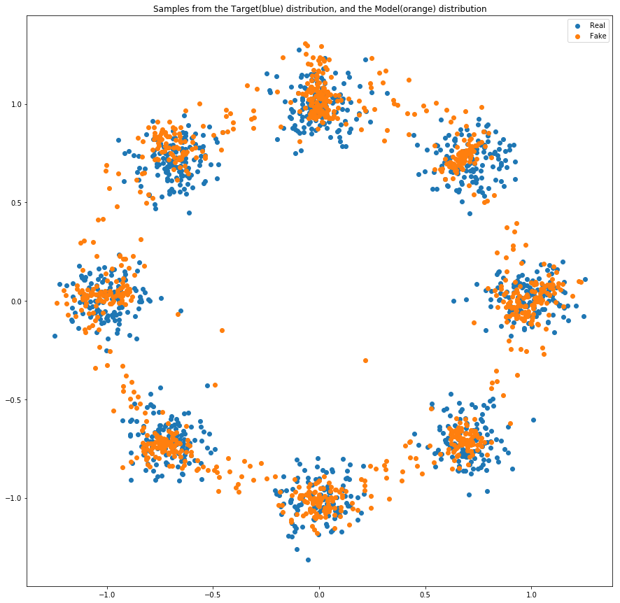
(a)

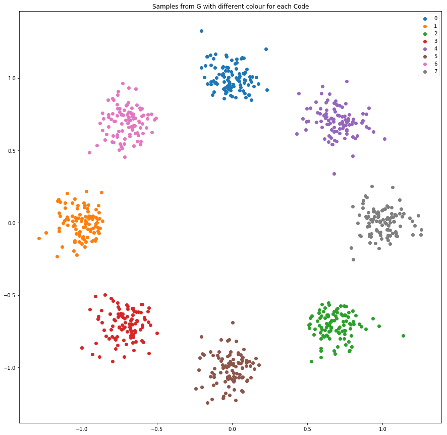
(b)

Figure 10: (a) GMAN: scatter plot of the data distribution (blue) and model distribution (orange). Although it is covering all the modes, there are a lot of false positives lying between the actual modes. (b) DoPaNet: scatter plot of the model distribution with different colors assigned for samples generated using different code. We sample $c$ from uniform categorical distribution. Notice that the modes are clearly separated from each other as compared to GMAN.

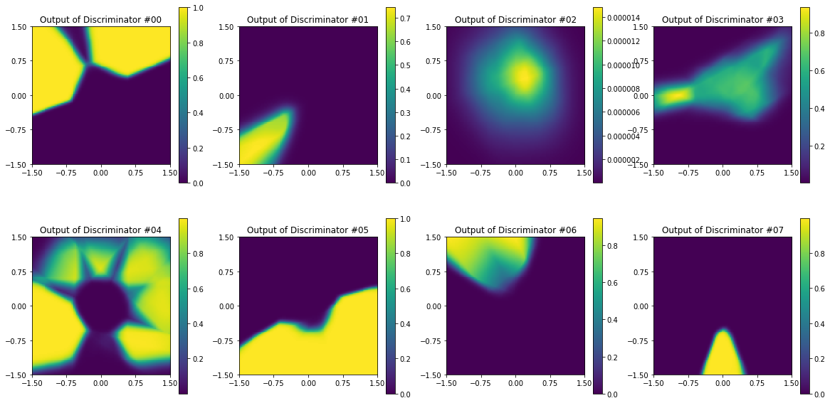
(a)

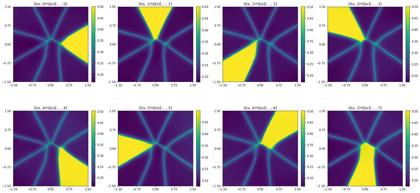
(b)

Figure 11: Heat map of discriminator scores $\in[0,1]$ ($0$ signifies fake while $1$ means real) when evaluated for every data-point pair lying in $\left[-1.5,1.5\right]^{2}$ (corresponding to Figure 10). (a) GMAN: it is clear that discriminator #04 already covers the majority of the modes while the other discriminators give high scores for obviously fake samples (#03 and #05). (b) DoPaNet: here we multiplied the discriminator scores with the probability of each point being assigned to that discriminator (obtained from classifier $Q$). Although the capacity of each discriminator in DoPaNet is identical to the discriminators in the GMAN experiment, the DoPaNet framework reduces the complexity of each discriminator’s task by making it work only on a different identifiable mode.

Appendix C CIFAR-10

As discussed in the Section 4.2.2, here we present some more results obtained for each of the $10$ classes of CIFAR-10 in Figure 12 and Figure 13.

Appendix D Implementation details

Here we present the way we structured our experiments and the details about the network architecture we used in the experiments.

D.1 Synthetic low dimensional distributions

First, we reproduced the 1D setting in (Ghosh et al., 2017) with 5 modes at $[10,20,60,80,110]$ and standard deviations $[3,3,2,2,1]$ respectively and we compare to the numbers reported in that paper in Table 1. Second, we compared DoPaNet directly to GMAN (Durugkar et al., 2017) qualitatively in Figure 5 and quantitatively in Table 3 using a circular 2D GMM distribution with 3 and 8 modes respecitvely, around the unit circle. To illustrate the advantage of DoPaNet over GMAN (Durugkar et al., 2017) we plotted the gradient field to visualize the benefit of using multiple discriminators. The gradient field of this setup can be seen in Figure 5. To get quantitative results, we estimated the probability density distribution using a histogram with 1400 bins over the real and generated samples and computed the Chi-square and KL-divergence between the two histograms.

Comparing against other GAN variants

When comparing against other GAN variants, we run the 1D experiments using a fixed set of 200,000 samples from the real distribution and generate 65,536 elements from each model.

Since DoPaNet is directly designed to separate different modes, we outperform all the other methods as shown in Table 1.

In our case, we sample the code vectors for the generator from a categorical distribution with uniform probability. For the best results, we use 5 discriminators in both GMAN (Durugkar et al., 2017) and DoPaNet. For both, we train 3 instances and select the best score from each of them.

Benchmarking the number of discriminators

In 1D for better non-parametric probability density estimation, we increased the number of generated samples from 65,536 to 1,000,000 samples as done in (Ghosh et al., 2017). For more reliable results on the implied mechanism of both approaches, we run the training 20 times for each algorithm with number of discriminators $N={2,\ldots,8}$, totaling 320 training. As in the previous experiment, we chose the best results from each run.

2D experiments

In 2D, for both variants we experiment with $M=N=8$ (where $N$ is the number of discriminators, $M$ is the number of Gaussians we used in the mixture) for quantitative results, listed in Table 3 and $M=N=3$ setting for qualitative results, illustrated in Figure 5. For each experiment we use a fixed set of 1,000,000 samples and take 5 run per each algorithm, then report the best run. We took effort to make sure that the comparison was fair, and used the same set of parameters as it was done in the 1D experiments.

D.2 Image generation

For both the generator and discriminator we use ResNet-architectures (He et al., 2016), with 18 layers each in the CIFAR-10 experiments, and 26 layers each in the CelebA experiments. As was done in (Mescheder, 2018) we multiply the output of the ResNet blocks with 0.1, use 256-dimensional unit Gaussian distribution. For categorical conditional image generation we use an embedding network that projects category indices to 256 dimensional label vector, normalized to the unit sphere. In the case of conditional image generation the classifier $Q$ is trained on code vectors, so it is constrained to learn the original class labels. We embed the code vector similar to the ground truth labels in this setting for CIFAR-10. We use Leaky-RELU nonlinearities everywhere, without BatchNorm.

Following the considerations in (Mescheder, 2018) for optimizing parameters of $Q$, $D$, $G$ we use the RMSProp with $\alpha=0.99$, $\epsilon=10^{-8}$, and initial learning rate of $10^{-3}$. We use a batch size of 64, and train the algorithm for 700,000 and 400,000 iterations for CIFAR-10 and CelebA tasks respectively. Similar to work that provided state of the art results on image generation tasks (Karras et al., 2018; Mescheder, 2018) for visualizing the generator’s progress we use an exponential moving average of the parameters of $G$ with decay 0.999.

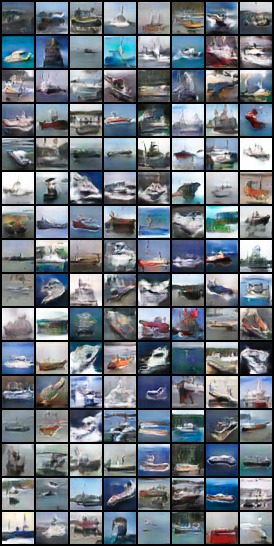
(a) Ship

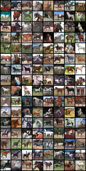
(b) Horse

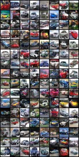
(c) Car

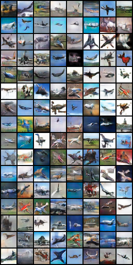
(d) Airplane

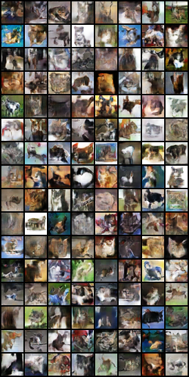
(e) Cat

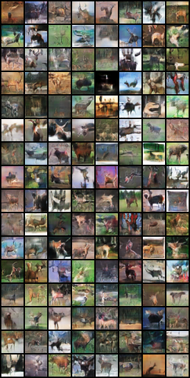
(f) Deer

Figure 12: $32\times 32$ CIFAR-10 samples drawn from DoPaNet trained with $N=5$ discriminators for 700k iterations. The generations in each subfigure correspond to $y=1,\dots,6$ respectively. We call the attention to the various different details learnt for each class which can cause mode collapse in other GAN variants.

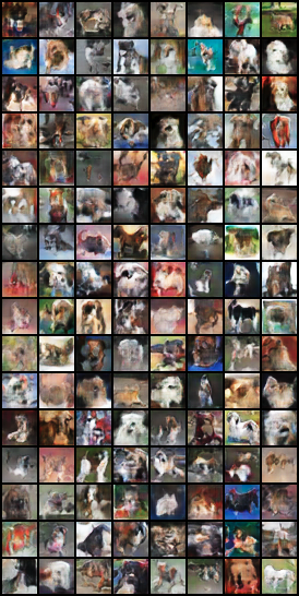
(a) Dog

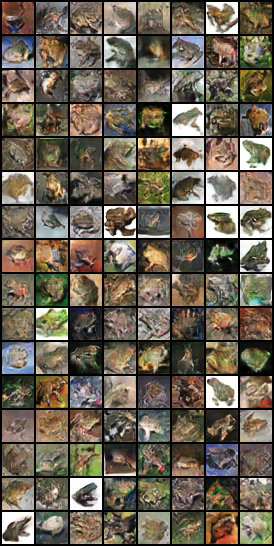
(b) Frog

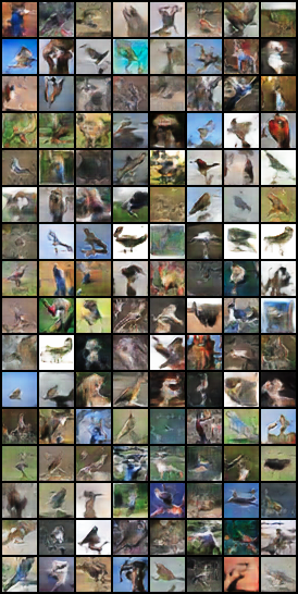
(c) Bird

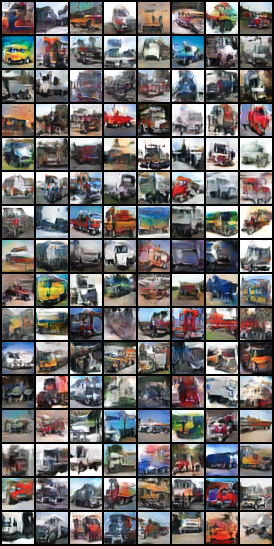
(d) Truck

Figure 13: $32\times 32$ CIFAR-10 samples drawn from DoPaNet trained with $N=5$ discriminators for 700k iterations. The generations in each subfigure correspond to $y=7,8,9$ and $10$ respectively. We call the attention to the various different details learnt for each class which can cause mode collapse in other GAN variants.

References

- Arjovsky & Bottou (2017) Arjovsky, M. and Bottou, L. Towards principled methods for training generative adversarial networks. In ICLR, 2017.
- Arjovsky et al. (2017) Arjovsky, M., Chintala, S., and Bottou, L. Wasserstein gan. arXiv preprint arXiv:1701.07875, 2017.
- Arora et al. (2017a) Arora, S., Ge, R., Liang, Y., Ma, T., and Zhang, Y. Generalization and equilibrium in generative adversarial nets (gans). In ICML, 2017a.
- Arora et al. (2017b) Arora, S., Ge, R., Liang, Y., Ma, T., and Zhang, Y. Generalization and equilibrium in generative adversarial nets (GANs). In Proceedings of the 34th International Conference on Machine Learning, 2017b.
- Berthelot et al. (2017) Berthelot, D., Schumm, T., and Metz, L. Began: boundary equilibrium generative adversarial networks. arXiv preprint arXiv:1703.10717, 2017.
- Che et al. (2017) Che, T., Li, Y., Jacob, A. P., Bengio, Y., and Li, W. Mode regularized generative adversarial networks. In ICLR, 2017.
- Chen et al. (2016) Chen, X., Duan, Y., Houthooft, R., Schulman, J., Sutskever, I., and Abbeel, P. Infogan: Interpretable representation learning by information maximizing generative adversarial nets. In NIPS, 2016.
- Donahue et al. (2017) Donahue, J., Krähenbühl, P., and Darrell, T. Adversarial feature learning. In ICLR, 2017.
- Durugkar et al. (2017) Durugkar, I., Gemp, I., and Mahadevan, S. Generative multi-adversarial networks. In ICLR, 2017.
- Ghosh et al. (2016) Ghosh, A., Kulharia, V., and Namboodiri, V. Message passing multi-agent gans. arXiv preprint arXiv:1612.01294, 2016.
- Ghosh et al. (2017) Ghosh, A., Kulharia, V., Namboodiri, V., Torr, P. H., and Dokania, P. K. Multi-agent diverse generative adversarial networks. arXiv preprint arXiv:1704.02906, 1(4), 2017.
- Goodfellow (2016) Goodfellow, I. Nips 2016 tutorial: Generative adversarial networks. arXiv preprint arXiv:1701.00160, 2016.
- Goodfellow et al. (2014a) Goodfellow, I., Pouget-Abadie, J., Mirza, M., Xu, B., Warde-Farley, D., Ozair, S., Courville, A., and Bengio, Y. Generative adversarial nets. In NIPS, 2014a.
- Goodfellow et al. (2014b) Goodfellow, I., Pouget-Abadie, J., Mirza, M., Xu, B., Warde-Farley, D., Ozair, S., Courville, A., and Bengio, Y. Generative adversarial nets. In Advances in neural information processing systems, pp. 2672–2680, 2014b.
- Gulrajani et al. (2017) Gulrajani, I., Ahmed, F., Arjovsky, M., Dumoulin, V., and Courville, A. C. Improved training of wasserstein gans. In NIPS, 2017.
- He et al. (2016) He, K., Zhang, X., Ren, S., and Sun, J. Deep residual learning for image recognition. In Proceedings of the IEEE conference on computer vision and pattern recognition, pp. 770–778, 2016.
- Juefei-Xu et al. (2017) Juefei-Xu, F., Boddeti, V. N., and Savvides, M. Gang of gans: Generative adversarial networks with maximum margin ranking. arXiv preprint arXiv:1704.04865, 2017.
- Karras et al. (2018) Karras, T., Aila, T., Laine, S., and Lehtinen, J. Progressive growing of gans for improved quality, stability, and variation. In ICLR, 2018.
- Ledig et al. (2017) Ledig, C., Theis, L., Huszár, F., Caballero, J., Cunningham, A., Acosta, A., Aitken, A. P., Tejani, A., Totz, J., Wang, Z., et al. Photo-realistic single image super-resolution using a generative adversarial network. In CVPR, 2017.
- Li et al. (2017) Li, C., Xu, K., Zhu, J., and Zhang, B. Triple generative adversarial nets. In NIPS, 2017.
- Liu & Tuzel (2016) Liu, M.-Y. and Tuzel, O. Coupled generative adversarial networks. In NIPS, 2016.
- Mescheder (2018) Mescheder, L. On the convergence properties of gan training. arXiv preprint arXiv:1801.04406, 2018.
- Mescheder et al. (2018) Mescheder, L., Nowozin, S., and Geiger, A. Which training methods for gans do actually converge? In International Conference on Machine Learning (ICML), 2018.
- Metz et al. (2017) Metz, L., Poole, B., Pfau, D., and Sohl-Dickstein, J. Unrolled generative adversarial networks. In ICLR, 2017.
- Mirza & Osindero (2014) Mirza, M. and Osindero, S. Conditional generative adversarial nets. arXiv preprint arXiv:1411.1784, 2014.
- Radford et al. (2016) Radford, A., Metz, L., and Chintala, S. Unsupervised representation learning with deep convolutional generative adversarial networks. In ICLR, 2016.
- Salimans et al. (2016) Salimans, T., Goodfellow, I., Zaremba, W., Cheung, V., Radford, A., and Chen, X. Improved techniques for training gans. In NIPS, 2016.
- Srivastava et al. (2017) Srivastava, A., Valkoz, L., Russell, C., Gutmann, M. U., and Sutton, C. Veegan: Reducing mode collapse in gans using implicit variational learning. In Advances in Neural Information Processing Systems, pp. 3308–3318, 2017.
- Vondrick et al. (2016) Vondrick, C., Pirsiavash, H., and Torralba, A. Generating videos with scene dynamics. In NIPS, 2016.
- Zhu et al. (2017) Zhu, J.-Y., Park, T., Isola, P., and Efros, A. A. Unpaired image-to-image translation using cycle-consistent adversarial networks. arXiv preprint, 2017.