Time and Energy-Optimal Lane Change Maneuvers for Cooperating Connected and Automated Vehicles^⋆

Abstract

We derive optimal control policies for a Connected and Automated Vehicle (CAV) cooperating with neighboring CAVs to implement a highway lane change maneuver. We optimize the maneuver time and subsequently minimize the associated energy consumption of all cooperating vehicles in this maneuver. We prove structural properties of the optimal policies which simplify the solution derivations and lead to analytical optimal control expressions. The solutions, when they exist, are guaranteed to satisfy safety constraints for all vehicles involved in the maneuver. Simulation results show the effectiveness of the proposed solution and significant performance improvements compared to maneuvers performed by human-driven vehicles.

I Introduction

Advances in next generation transportation system technologies and the emergence of Connected and Automated Vehicles (CAVs), also known as “autonomous vehicles”, have the potential to drastically improve a transportation network’s performance in terms of safety, comfort, congestion reduction and energy efficiency. In highway driving, an overview of automated intelligent vehicle-highway systems was provided in [1] with more recent developments mostly focusing on autonomous car-following control [2],[3],[4]. Automating a lane change maneuver remains a challenging problem which has attracted increasing attention in recent years [5],[6],[7],[8].

The basic architecture of an automated lane-change maneuver can be divided into the strategy level and the control level [9]. The strategy level generates a feasible (possibly optimal in some sense) trajectory for a lane-change maneuver. The control level is responsible for determining how vehicles track the aforementioned trajectory. For example, [7] adopts such an architecture for an automated lane-change maneuver, but does not provide an analytical solution and assumes that there are no other vehicles in the left lane (the lane in which the controllable vehicle ends up after completing the maneuver). In [10], background vehicles are included in the left lane and the goal is to check whether there exists a lane-change trajectory or not; if one exists, the controllable vehicle will then track this trajectory. A similar approach is taken in [11] with the trajectory being updated during the maneuver based on the latest surrounding information. In these papers, only one vehicle can be controlled during the maneuver and no analytical solutions are provided.

The emergence of CAVs brings up the opportunity for cooperation among vehicles traveling in both left and right lanes in carrying out an automated lane-change maneuver [9],[12],[13]. Such cooperation presents several advantages relative to the two-level architecture mentioned above. In particular, when controlling a single vehicle and checking on the feasibility of a maneuver depending on the state of the surrounding traffic, as in [14],[15], the maneuver may be infeasible without the cooperation of other vehicles, especially under heavier traffic conditions. In contrast, a cooperative architecture can allow multiple interacting vehicles to implement controllers enabling a larger set of maneuvers. This cooperative behavior can also improve the throughput, hence reducing the chance of congestion. Feasible, but not necessarily optimal, vehicle trajectories for cooperative multi-agent lane-changing maneuvers are derived in [16]. The case of multiple cooperating vehicles simultaneously changing lanes is considered in [17] with the requirement that all vehicles are controllable and their velocities prior to the lane change are all the same. First, vehicles with a lower priority must adjust their positions in their current lane and give way to those with a higher priority so as to avoid collisions. Then, a lane changing optimal control problem is solved for each vehicle without considering the usual safe distance constraints between vehicles. This “progressively constrained dynamic optimization” method facilitates a numerical solution to the underlying optimal control problem at the expense of some loss in performance.

Our goal is to provide an optimal solution for the maneuver in Fig. 1, in which the controlled vehicle $C$ attempts to overtake an uncontrollable vehicle $U$ by using the left lane to pass. In this case, the initial velocities of all vehicles can be different and arbitrary.

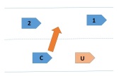
Figure 1: The basic lane changing maneuver process.

The overall lane changing and passing maneuver consists of three steps: $(i)$ The target vehicle $C$ moves to the left lane, $(ii)$ $C$ moves faster than $U$ (and possibly other vehicles ahead of it) while on the left lane, $(iii)$ $C$ moves back to the right lane. The first step is further subdivided into two parts. First, vehicle $C$ adjusts its position in the current lane to prepare for a lane shift, while vehicles $1$ and $2$ in Fig. 1 cooperate to create space for $C$ in the left lane. Next, the latitudinal lane shift of $C$ takes place. In this paper, we limit ourselves to the first part of step $(i)$. Our objective is to minimize both the maneuver time and the energy consumption of vehicles $C$, $1$ and $2$ which are all assumed to share their state information. We also impose a hard safe distance constraint between all adjacent vehicles located in the same lane, as well as constraints due to speed and acceleration limits imposed on all vehicles. We first determine a minimum feasible time for the maneuver (if one exists) and associated terminal positions for vehicles $C$, $1$ and $2$. We then solve a fixed terminal time decentralized optimal control problem for each of the three vehicles. We derive several properties of the optimal solution which facilitate obtaining explicit analytical solutions, hence leading to real-time implementability. Our approach applies to a wider range of scenarios relative to those in [10],[11],[14],[15] and incorporates the safety distance constraint not included in [16] and [17].

The rest of this paper is organized as follows. Section II formulates the lane-change maneuver problem. In Section III, a complete optimal control solution is obtained. Section IV provides simulation results for several representative examples and we conclude with Section V.

II Problem Formulation

We define $x_{i}(t)$ to be the longitudinal position of vehicle $i$ along its current lane measured with respect to a given origin, where we use $i=1,2,C,U$. Similarly, $v_{i}(t)$ and $u_{i}(t)$ are vehicle $i$’s velocity and (controllable) acceleration. The dynamics of vehicle $i$ are

$$\vspace*{0pt}\dot{x}_{i}(t)=v_{i}(t),\text{ \ \ }\dot{v}_{i}(t)=u_{i}(t)$$ (1)

The maneuvers carried out by vehicles $1,2,C$ are initiated at time $t_{0}$ and end at time $t_{f}$. We define $d_{i}(v_{i}(t))$ to be the minimal safe distance between vehicle $i$ and the one that precedes it in its lane, which in general depends on the vehicle’s current speed. The control input and speed are constrained as follows for all $t\in[t_{0},t_{f}]$:

$$u_{i\text{min}}\leq u_{i}(t)\leq u_{i\text{max}},\text{ \ \ }v_{i\text{min}}\leq v_{i}(t)\leq v_{i\text{max}}$$ (2)

where $u_{i\text{max}}$, $u_{i\text{min}}$, $v_{i\text{max}}$, $v_{i\text{min}}$ are the maximal and minimal acceleration (respectively speed) limits. In Fig. 1, we control vehicles $1$, $2$ and $C$ to complete a lane change maneuver while minimizing the maneuver time and the corresponding energy consumption. For each vehicle $i=1,2,C$ we formulate the following optimization problem assuming that $x_{i}(0)$ and $v_{i}(0)$ are given:

$$J(t_{f};u_{i}(t))= \min_{u_{i}(t)}\int_{0}^{t_{f}}[w_{t}+$$ (3)

$$[w_{1,u}u_{1}^{2}(t)+w_{2,u}u_{2}^{2}(t)+w_{C,u}u_{C}^{2}(t)]]dt$$

s.t.  (1), (2) and

$$x_{1}(t)-x_{2}(t) >d_{2}(v_{2}(t)),\text{ \ }t\in[0,t_{f}]$$

$$x_{U}(t)-x_{C}(t) >d_{C}(v_{C}(t)),\text{ \ }t\in[0,t_{f}]$$

$$x_{1}(t_{f})-x_{C}(t_{f}) >d_{C}(v_{C}(t_{f})),\text{ \ \ }x_{C}(t_{f})-x_{2}(t_{f})>d_{2}(v_{2}(t_{f}))$$

where $w_{t}$, $w_{u}$ are weights associated with the maneuver time $t_{f}$ and with a measure of the total energy expended. The two terms in the previous function need to be properly normalized and we set $w_{t}=\frac{\rho}{T_{\max}}$ and $w_{i,u}=\frac{1-\rho}{\text{max}\{u_{\text{imax}}^{2},u_{\text{imin}}^{2}\}}$, where $\rho\in[0,1]$ and $T_{\max}$ is a prespecified upper bound on the maneuver time (e.g., $T_{\max}=l/\min\{v_{\text{imin}}\}$, $i=1,2,C,U$, where $l$ is the distance to the next highway exit). Clearly, if $\rho=0$ this problem reduces to an energy minimization problem and if $\rho=1$ it reduces to minimizing the maneuver time. The safe distance is defined as $d_{i}(v_{i}(t))=\phi v_{i}(t)+\delta$ where $\phi$ is the headway time (the general rule $\phi=1.8$ is usually adopted as in [18]). As stated, the problem allows for a free terminal time $t_{f}$ and terminal state constraints $x_{i}(t_{f})$, $v_{i}(t_{f})$. We will next specify the terminal time $t_{f}$ as the solution of a minimization problem which allows each vehicle to specify a desired “aggressiveness level” relative to the shortest possible maneuver time subject to (2). Then, we will also specify $x_{i}(t_{f})$, $i=1,2,C$.

III Optimal Control Solution

Terminal time specification. We begin by formulating the following minimization problem based on which the maneuver terminal time $t_{f}$ is specified:

$$\min_{t_{f}>0}\text{ }t_{f}$$ (4)

$$\text{ s.t. }x_{1}(0) +v_{1}(0)t_{f}+0.5\alpha_{1}u_{1\text{max}}t_{f}^{2}$$

$$- x_{C}(0)-v_{C}(0)t_{f}-0.5\alpha_{C}u_{C\text{max}}t_{f}^{2}>d_{C}(v_{C}(t_{f}))$$ (4a)

$$x_{U}(t_{f}) -x_{C}(0)-v_{C}(0)t_{f}$$

$$- 0.5\alpha_{C}u_{C\text{min}}t_{f}^{2}>d_{C}(v_{C}(t_{f}))$$ (4b)

$$x_{C}(0) +v_{C}(0)t_{f}+0.5\alpha_{C}u_{C\text{min}}t_{f}^{2}$$

$$- x_{2}(0)-v_{2}(0)t_{f}-0.5\alpha_{2}u_{2\text{min}}t_{f}^{2}>d_{2}(v_{2}(t_{f}))$$ (4c)

where $\alpha_{i}\in[0,1),i=1,2,C$ is an “aggressiveness coefficient” for vehicle $i$ which can be preset by the driver. Observe that $[x_{i}(t_{0})+v_{i}(t_{0})t_{f}+0.5\alpha_{i}u_{i\text{max}}t_{f}^{2}]$ is the terminal position of $i$ under control $\alpha_{i}u_{i\text{max}}$. To minimize $t_{f}$, vehicle $1$ should accelerate and vehicle $2$ decelerate so as to increase the gap between them in Fig. 1. If $C$ accelerates, then (4a) ensures the safety constraint is still satisfied. If $C$ has to decelerate because it is constrained by $U$, then (4b) ensures that the safety constraint between $U$ and $C$ is satisfied and (4c) ensures that the safety constraint between $2$ and $C$ is also satisfied. As we will subsequently show, the optimal control of $C$ is either always non-positive or always non-negative throughout $[0,t_{f}]$ so that either the first or the last two constraints are relevant to it. Naturally, a solution to (4) may not exist, in which case we must iterate on the values of $\alpha_{i}$ until one is possibly identified. If that is not possible, then the maneuver is clearly aborted. If $t_{f}$ exists, we will specify terminal position $x_{i}(t_{f})$ next and check the feasibility of $(x_{i,f},t_{f})$ later in this section.

Terminal position specifications. Assuming a solution $t_{f}$ is determined, we next seek to specify terminal vehicle positions $x_{i}(t_{f}),$ $i=1,2,C$, to be associated with problem (LABEL:cost_function). To do so, we define

$$\Delta x_{i}(t_{f})=x_{i}(t_{f})-x_{i}(t_{0})-v_{i}(t_{0})t_{f}$$

which is the difference between the actual terminal position of $i$ and its ideal terminal position under constant speed $v_{i}(t_{0})$; this is ideal from the energy point of view in (5), since the energy component is minimized when $u_{i}(t)=0$. Thus, the energy-optimal value is $\Delta x_{i}(t_{f})=0$. We then seek terminal positions that minimize a measure of deviating form these energy-optimal values over all three vehicles:

$$\min_{x_{i}(t_{f})>x_{i}(0),i=1,2,C} \Delta x^{2}_{C}(t_{f})+\Delta x^{2}_{1}(t_{f})+\Delta x^{2}_{2}(t_{f})$$ (5)

s.t. $$\Delta x_{i}(t_{f})=x_{i}(t_{f})-x_{i}(0)-v_{i}(t_{0})t_{f}$$

$$x_{1}(t_{f})-x_{C}(t_{f})>\max\{d_{C}(v_{C}(t))\}$$

$$x_{C}(t_{f})-x_{2}(t_{f})>\max\{d_{2}(v_{2}(t))\}$$

$$x_{U}(t_{f})-x_{C}(t_{f})>\max\{d_{C}(v_{C}(t))\}$$

The max values in (5) are assumed to be given by a prespecified maximum inter-vehicle safe distance. However, as subsequently shown in Theorem $1$, they actually turn out to be the known initial or terminal values of $d_{2}(v_{2}(t))$ and $d_{C}(v_{C}(t))$. For example, $\max\{d_{2}(v_{2}(t))\}=d_{2}(v_{2}(t_{0}))$ and $\max\{d_{C}(v_{C}(t))\}=d_{C}(v_{C}(t_{0})+u_{C\max}t_{f})$.

Lemma $1$: The solution $x_{i}^{\ast}(t_{f})$, $i=1,2,C$, to (5) satisfies $\Delta x_{1}^{\ast}(t_{f})\geq 0$ and $\Delta x_{2}^{\ast}(t_{f})\leq 0$.

Proof: If $\Delta x_{1}^{\ast}(t_{f})<0$, then $\Delta x_{1}(t_{f})=0$ is a better solution since it is feasible (the distance between vehicles $1$, $2$ under $\Delta x_{1}(t_{f})=0$ is larger than under $\Delta x_{1}^{\ast}(t_{f})<0$) and it is obvious that it yields a lower cost in (5) than the one with $\Delta x_{1}^{\ast}(t_{f})<0$ (the control is $u_{i}(t)=0$.) Therefore, we must have $\Delta x_{1}^{\ast}(t_{f})\geq 0$. The proof for $\Delta x_{2}^{\ast}(t_{f})\leq 0$ is similar. $\blacksquare$

III-A Optimal Control of Vehicles $1$ and $2$

With the terminal time $t_{f}$ and longitudinal position $x_{i}(t_{f})$, $i=1,2$, set through (4) and (5) respectively, the optimal control problems of vehicles $i=1,2$ in (LABEL:cost_function) become:

$$\min_{u_{1}(t)}\int_{0}^{t_{f}}\frac{1}{2}u_{1}^{2}(t)dt\text{ \ \ \ s.t. \ (\ref{vehicle_dynamics}), (\ref{vehicle_constraint}), }x_{1}(t_{f})=x_{1,f}$$ (6)

$$\min_{u_{2}(t)}\int_{0}^{t_{f}}\frac{1}{2}u_{2}^{2}(t)dt\text{ \ \ \ s.t. \ (\ref{vehicle_dynamics}), (\ref{vehicle_constraint}), }x_{2}(t_{f})\leq x_{2,f},$$ (7)

$$x_{1}(t)-x_{2}(t)>d_{2}(v_{2}(t)),\text{ \ }t\in[0,t_{f}]$$

where $x_{1,f}$ and $x_{2,f}$ are given above. In (7), we use an inequality $x_{2}(t_{f})\leq x_{2,f}$ to describe the terminal position constraint instead of the equality since it suffices for the distance between the two vehicles to accommodate vehicle $C$ while at the same time allowing for the cost under a control with $x_{2}(t_{f})<x_{2,f}$ to be smaller than under a control with $x_{2}(t_{f})=x_{2,f}$. In (6), there is no need to consider the case that $x_{1}(t_{f})>x_{1,f}$ since it is clear that the optimal cost when $x_{1}(t_{f})=x_{1,f}$ is always smaller compared to $x_{1}(t_{f})>x_{1,f}$. The next result establishes the fact that the solution of these two problems involves vehicle 1 never decelerating and vehicle 2 never accelerating.

Theorem $1$ The optimal control in (6) is $u_{1}^{\ast}(t)\geq 0$ and the optimal control in (7) is $u_{2}^{\ast}(t)\leq 0$.

Proof: First, by Lemma $1$, it is obvious that $u_{1}(t)\geq 0$ is a feasible solution of (6) since $\Delta x_{1}^{\ast}(t_{f})\geq 0$ implies that $u_{1}(t)<0$ for all $t\in[t_{0},t_{f}]$ is not feasible. The same applies to $u_{2}(t)\leq 0$ being a feasible solution of (7).

Starting with vehicle $1$, suppose that there exists some $[t_{1},t_{2})\subset[0,t_{f}]$ in which the optimal solution satisfies $u_{1}^{\ast}(t)<0$. We will show that there exists another control which would lead to a smaller cost than $u_{1}^{\ast}(t)$. Consider a control $u_{1}^{1}(t)$ defined so that $u_{1}^{1}(t)=u_{1}^{\ast}(t)\geq 0$ for $t\in[0,t_{1})\cup[t_{2},t_{f}]$, $u_{1}^{1}(t)=0$ for $t\in[t_{1},t_{2})$. It is obvious that the cost of the control $u_{1}^{1}(t)$ is lower than that of $u_{1}^{\ast}(t)$. However, we have $x_{1}^{1}(t_{f})>x_{1}^{\ast}(t_{f})$ because $u_{1}^{1}(t)>u_{1}^{\ast}(t)$, $t\in[t_{1},t_{2})$, thus violating the terminal condition in (6). Therefore, we construct another control $u_{1}^{2}(t)$, a variant of $u_{1}^{1}(t)$ which is feasible, as follows. Define

$$g_{1}(t)=x_{1}^{1}(t)+v_{1}^{1}(t)(t_{f}-t)$$ (8)

and observe that $g_{1}(t)$ is a continuous function of $t$ since $x_{1}^{1}(t)$ and $v_{1}^{1}(t)$ are continuous. Because $g_{1}(0)={x}_{1}^{1}(0)+v_{1}^{1}(0)t_{f}<x_{1}^{\ast}(t_{f})$ (by Lemma $1$) and $g_{1}(t_{f})=x_{1}^{1}(t_{f})\geq x_{1}^{\ast}(t_{f})$, there exists some $t_{m}\in[0,t_{f}]$ such that $g_{1}(t_{m})=x_{1}^{\ast}(t_{f})$. We now define a control $u_{1}^{2}(t)$ such that $u_{1}^{2}(t)=u_{1}^{1}(t)\geq 0$ for $t\in[0,t_{m})$, $u_{1}^{2}(t)=0$ for $t\in[t_{m},t_{f}]$. It follows that $x_{1}^{2}(t_{m})=x_{1}^{1}(t_{m})$, $v_{1}^{2}(t_{m})=v_{1}^{1}(t_{m})$ and $x_{1}^{2}(t_{f})=x_{1}^{1}(t_{m})+v_{1}^{1}(t_{m})(t_{f}-t_{m})$ which implies that $x_{1}^{2}(t_{f})=g_{1}(t_{m})$ from (8). Thus, the terminal position constraint is not violated under $u_{1}^{2}(t)$. Based on the definitions of $u_{1}^{2}(t)$ and $u_{1}^{1}(t)$, it is obvious that $u_{1}^{2}(t)$ does not violate the acceleration constraints in (2). Next, we show that the velocity constraints in (2) are also not violated. Assume that for some $t_{n}$, $v_{1}^{1}(t_{n})=v_{\text{1max}}$ initiating an arc where the velocity is $v_{1}^{1}(t)=v_{\text{1max}}$. There are two cases:

(a) If $t_{n}\geq t_{m}$, we have $v_{1}^{1}(t_{m})\leq v_{1}^{1}(t_{n})$ because $u_{1}^{1}(t)\geq 0$ for all $t\in[0,t_{f}]$. Based on the definition of $u_{1}^{2}(t)$, the maximal speed under the control $u_{1}^{2}(t)$ is $v_{1}^{1}(t_{m})$ and the velocity constraint is, therefore, inactive.

(b) If $t_{n}<t_{m}$, we have $v_{1}^{1}(t_{m})>v_{1}^{1}(t_{n})$. Taking the time derivative of $g_{1}(t)$, we get $\dot{g}_{1}(t)=u_{1}^{1}(t)(t_{f}-t)\geq 0$. It follows that

$$g_{1}(t_{n})<g_{1}(t_{m})=x_{1}^{\ast}(t_{f})$$ (9)

where the equality follows from the definition of $t_{m}$ above. Then, let us construct a new control $u_{1}^{3}(t)$ such that $u_{1}^{3}(t)=u_{1}^{\ast}(t)\geq 0$ for $t\in[0,t_{1})\cup[t_{2},t_{n})$, $u_{1}^{3}(t)=0$ for $t\in[t_{1},t_{2})\cup[t_{n},t_{f}]$, where $t_{n}\geq t_{1}$ because $v_{1}^{3}(t)<v_{\text{1max}}$ for $t<t_{1}$ based on the feasibility of $u_{1}^{\ast}(t)$. Moreover, if $t_{1}<t_{n}<t_{2}$, we define $u_{1}^{3}(t)=0$ for $t>t_{1}$, i.e., $u_{1}^{3}(t)=u_{1}^{\ast}(t)\geq 0$ for $t\in[0,t_{1})$, $u_{1}^{3}(t)=0$ for $t\in[t_{1},t_{f}]$. Based on the definition of $u_{1}^{3}(t)$, we have $u_{1}^{3}(t)=u_{1}^{1}(t)$ for $t\in[0,t_{n})$. Therefore, $x_{1}^{3}(t_{n})=x_{1}^{1}(t_{n})$ and $v_{1}^{3}(t_{n})=v_{1}^{1}(t_{n})$ so that (9) holds under $u_{1}^{3}(t)$. When $t\geq t_{n}$, we have $u_{1}^{3}(t)=0$, therefore, $x_{1}^{3}(t_{f})=x_{1}^{1}(t_{n})+v_{1}^{1}(t_{n})(t_{f}-t_{n})=g_{1}(t_{n})$ from (8). Since $v_{1}^{3}(t)=v_{1\text{max}}$ for $t\in[t_{n},t_{f}]$ and $x_{1}^{3}(t)\geq x_{1}^{\ast}(t)$ for $t\in[0,t_{n})$, it is clear that $x_{1}^{3}(t_{f})\geq x_{1}^{\ast}(t_{f})$. However, since $g_{1}(t_{n})=x_{1}^{3}(t_{f})\geq x_{1}^{\ast}(t_{f})$, this contradicts (9). We conclude that $t_{n}<t_{m}$ is not possible. In summary, we have shown that the velocity constraint is inactive for control $u_{1}^{2}(t)$. Therefore, $u_{1}^{2}(t)$ is feasible and results in a lower cost in (6) than $u_{1}^{\ast}(t)$ since it includes a trajectory arc over which $u_{1}^{2}(t)=0$. This contradicts the optimality of $u_{1}^{\ast}(t)$ and we conclude that the optimal control cannot contain any interval over which $u_{1}^{\ast}(t)<0$.

Next, consider vehicle 2 and suppose that there exists some $[t_{1},t_{2})\subset[0,t_{f}]$ in which the optimal solution satisfies $u_{2}^{\ast}(t)>0$. Consider a control $u_{2}^{1}(t)$ defined so that $u_{2}^{1}(t)=u_{2}^{\ast}(t)\leq 0$ for $t\in[0,t_{1})\cup[t_{2},t_{f}]$, $u_{1}^{1}(t)=0$ for $t\in[t_{1},t_{2})$. It is clear that the cost under $u_{2}^{1}(t)$ is lower than that of $u_{2}^{\ast}(t)$ and that the acceleration constraint in (2) is inactive for $u_{2}^{1}(t)$. Furthermore, it is obvious that $x_{2}^{\ast}(t)\geq x_{2}^{1}(t)$ and $v_{2}^{\ast}(t)\geq v_{2}^{1}(t)$ for $t\in[0,t_{f}]$. Therefore, the terminal position inequality in (7) is not violated. Based on the definition of the safety distance constraint, $d_{2}(v_{2}(t))$$=\phi v_{2}(t)+\delta$ is monotonically increasing in $v_{2}(t)$. Therefore, we conclude that the safety constraint under $u_{2}^{1}(t)$ will not be violated, since $u_{2}^{\ast}(t)$ is feasible and $x_{2}^{\ast}(t)\geq x_{2}^{1}(t)$, $v_{2}^{\ast}(t)\geq v_{2}^{1}(t)$. Finally, we consider the speed constraint in (2) which may be active under $u_{2}^{1}(t)$. There are two cases:

(a) If $v_{2}^{1}(t_{f})>v_{2\text{min}}$, the speed constraint is inactive under $u_{2}^{1}(t)$ over all $t\in[0,t_{f}]$ and $u_{2}^{1}(t)$ is a feasible solution which results in a lower cost in (7) than $u_{2}^{\ast}(t)$ since it includes a trajectory arc over which $u_{2}^{2}(t)=0$.

(b) If $v_{2}^{1}(t_{f})\leq v_{2\text{min}}$, there must exist some $t_{n}\in[t_{1},t_{f}]$ such that $v_{2}^{1}(t_{m})=v_{\text{2min}}$. Let us construct a new control ${u}_{2}^{2}(t)$ as follows: ${u}_{2}^{2}(t)=u_{2}^{1}(t)\leq 0$ for $t\in[0,t_{m})$, ${u}_{2}^{2}(t)=0$ for $t\in[t_{m},t_{f}]$. For $t\in[0,t_{m})$, it is obvious that $x_{2}^{\ast}(t)\geq x_{2}^{2}(t)$ and $v_{2}^{\ast}(t)\geq v_{2}^{2}(t)$ based on the definition of $u_{2}^{1}(t)$. For $t\in[t_{m},t_{f}]$, vehicle $2$ moves at the minimal speed $v_{2\text{min}}$ under $u_{2}^{2}(t)$, therefore, $x_{2}^{\ast}(t_{f})\geq x_{2}^{2}(t_{f})$, that is, the terminal position inequality is satisfied. Also, it is obvious that the acceleration and the speed constraints are not violated over $[0,t_{f}]$. Finally, we have shown that $u_{2}^{1}(t)$ does not violate the safety constraint. Based on the same argument, it is straightforward to show that $u_{2}^{2}(t)$ will not violate this constraint, since $x_{2}^{2}(t)\leq x_{2}^{\ast}(t)$ and $v_{2}^{2}(t)\leq v_{2}^{\ast}(t)$. Therefore, $u_{2}^{2}(t)$ is feasible in (7) and the corresponding cost is lower than that of $u_{2}^{\ast}(t)$ because the trajectory segment with $u_{2}^{2}(t)=0$ contributes to zero cost. We conclude that the optimal control $u_{2}^{\ast}(t)$ cannot contain any time interval with $u_{2}^{\ast}(t)>0$. $\blacksquare$

Based on Theorem $1$, in addition to showing that vehicle 1 never decelerates and vehicle 2 never accelerates, we also eliminate the safe distance constraint in (7) since the distance between the vehicles will increase in the course of the maneuver and the last two safety constraints in (LABEL:cost_function) ensure that this distance is eventually large enough to accommodate the length of vehicle $C$. Thus, (7) becomes

$$\min_{u_{2}(t)}\int_{0}^{t_{f}}\frac{1}{2}u_{2}^{2}(t)dt\text{ \ \ \ s.t. \ (\ref{vehicle_dynamics}), (\ref{vehicle_constraint}), }x_{2}(t_{f})=x_{2,f}$$ (10)

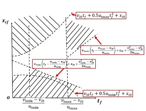
Figure 2: The feasible state set of controllable vehicles in the left lane.

Feasible terminal state set. The constraints in (2) limit the sets of feasible terminal conditions $(x_{i,f},t_{f})$, $i=1,2,C$ as shown in Fig. 2 where the feasible set is the unshaded area defined as follows for each $i=1,2,C$: $(i)$ Vehicle $i$ cannot reach $x_{i,f}$ under its maximal acceleration if $u_{i\max}t_{f}+v_{i,0}\leq v_{i\max}$ and $v_{i,0}t_{f}+0.5u_{i\max}t_{f}^{2}<x_{i,f}-x_{i,0}$. $(ii)$ Vehicle $i$ cannot reach $x_{i,f}$ under its maximal acceleration after attaining its maximal velocity if $u_{i\text{max}}t_{f}+v_{i,0}>v_{i\text{max}}$ and $v_{i\text{max}}(t_{f}-\frac{v_{i\text{max}}-v_{i,0}}{u_{i\text{max}}})<x_{i,f}-x_{i,0}-\frac{v_{i\text{max}}^{2}-v_{i,0}^{2}}{2u_{i\text{max}}}$. $(iii)$ Vehicle $i$ exceeds $x_{i,f}$ under the minimal acceleration if $u_{i\text{min}}t_{f}+v_{i,0}\geq v_{i\text{min}}$ and $v_{i,0}t_{f}+0.5u_{i\text{min}}t_{f}^{2}>x_{i,f}-x_{i,0}$. $(iv)$ Vehicle $i$ exceeds $x_{i,f}$ under the minimal acceleration after attaining its minimal velocity if $u_{i\text{min}}t_{f}+v_{i,0}<v_{i\text{min}}$ and $v_{i\text{min}}(t_{f}-\frac{v_{i\text{min}}-v_{i,0}}{u_{i\text{min}}})>x_{i,f}-x_{i,0}-\frac{v_{i\text{min}}^{2}-v_{i,0}^{2}}{2u_{i\text{min}}}$. In addition, vehicle $C$ must also satisfy a safety distance constraint with respect to vehicle $U$, hence if $x_{C,f}>x_{U}(0)+v_{U}t_{f}-d_{C}(v_{2}(t_{f}))$, there is no feasible solution.

Note that if an optimal $t_{f}$ is determined in (4) and the solution of (5) guarantees that $x_{i}(t_{f})$, $i=1,2,C$, do not violate the safety constraints, $(x_{i,f},t_{f})$ is expected to be feasible. However, if $(x_{i,f},t_{f})$ is infeasible for vehicle $i$, then the following algorithm is used to find a feasible such pair:

Algorithm 1:

(1) $t_{f}$ is updated using $t_{f}=\beta t_{f}$, $\beta>1$.

(2) With updated $t_{f}$, (5) is re-solved to obtain new $x_{i,f}$.

(3) If $(x_{i,f},t_{f})$ is feasible in Fig. 2, stop; else return to step (1) with a higher value of $\beta$.

In the above, the coefficient $\beta$ is used to relax the maneuver time $t_{f}$ so as to accommodate one or more of the constraints in Fig. 2 until a feasible $(x_{i,f},t_{f})$ is identified.

Solution of problem (6). We can now proceed to derive an explicit solution for (6) taking advantage of Theorem $1$. We begin by writing the Hamiltionian and associated Lagrangian functions for (6):

$$H(v_{1},u_{1},\lambda)=\frac{1}{2}u_{1}^{2}(t)+\lambda_{x}(t)v_{1}(t)+\lambda_{v}(t)u_{1}(t)$$ (11)

$$L(v_{1},u_{1},\lambda,\eta)= H(v,u,\lambda)+\eta_{1}(t)(u_{\text{1min}}-u_{1}(t))$$ (12)

$$+\eta_{2}(t)(u_{1}(t)-u_{\text{1max}})+\eta_{3}(t)(v_{\text{1min}}-v_{1}(t))$$

$$+\eta_{4}(t)(v_{1}(t)-v_{\text{1max}})$$

where $\lambda(t)=[\lambda_{v}(t),\lambda_{x}(t)]^{T}$ and $\eta=[\eta_{1}(t),...,\eta_{4}(t)]^{T}$. In view of Theorem 1, i.e., $u_{1}^{\ast}(t)\geq 0$, (12) reduces to

$$L(v_{1},u_{1},\lambda,\eta)= \frac{1}{2}u_{1}^{2}(t)+\lambda_{x}(t)v_{1}(t)+\lambda_{v}(t)u_{1}(t)$$ (13)

$$+\eta_{2}(t)(u_{1}(t)-u_{\text{1max}})+\eta_{3}(t)(v_{\text{1min}}-v_{1}(t))$$

$$+\eta_{4}(t)(v_{1}(t)-v_{\text{1max}})$$

The explicit solution of (6) is given next.

Theorem $2$ Let $x_{1}^{\ast}(t)$, $v_{1}^{\ast}(t)$, $u_{1}^{\ast}(t)$ be a solution of (6). Then,

$$u_{1}^{\ast}(t)=\arg\min_{0\leq u_{1}\leq u_{1\text{max}}}\frac{1}{2}[u_{1}^{2}+\dfrac{u_{1}^{\ast}(t_{0})^{2}(t-\tau)u_{1}}{v_{1,0}-v_{1}^{\ast}(t_{f})+(\tau-t_{0})u_{1}^{\ast}(t_{0})}]$$ (14)

where $\tau$ is the first time that $v_{1}^{\ast}(\tau)=v_{1\text{max}}$ and $\tau=t_{f}$ if $v_{1\text{max}}$ is never reached.

Proof: Problem (6) is of the same form as the fixed terminal time optimal control Problem 3 in [19] whose solution when $u_{1}^{\ast}(t)\geq 0$ is given in Theorem 2 of [19] and is therefore omitted. By Pontryagin’s principle applied to (11), $u_{1}^{\ast}(t)=$min$\{u_{1\max},{-\lambda_{v}(t)}\}$ and the key parts of the proof in [19] are showing that $\eta_{3}(t)=0$ and that $\lambda_{v}(t)$ is continuous for all $t\in[0,t_{f}]$. $\blacksquare$

Furthermore, following a derivation similar to that in [19] we can obtain the optimal cost $J_{1}^{\ast}(t_{f})$ in (6) based on several cases depending on the initial acceleration $u_{1,0}^{\ast}$ and the terminal velocity $v_{1}^{\ast}(t_{f})$ which can be explicitly evaluated as in [19]. The final optimal cost is the minimal among all possible values obtained.

Case I: $u_{1,0}^{\ast}=u_{1\text{max}}$ and $\dot{u}_{1}^{\ast}(t)=0$. If $t_{f}<\frac{v_{1\text{max}}-v_{1,0}}{u_{1\text{max}}}$, then $u_{1}^{\ast}(t)=u_{1\text{max}}$ for all $t\in[0,t_{f}]$. Otherwise, when $v_{1}(t)=v_{1\text{max}}$, the control switches to $u_{1}^{\ast}(t)=0$. Therefore,

$$J_{1}^{\ast}(t_{f})=\left\{\vspace*{0pt}\begin{array}[c]{l}\frac{1}{2}u_{1\text{max}}(v_{1\text{max}}-v_{1,0})\\ \frac{1}{2}u_{1\text{max}}^{2}(t_{f}-t_{0})\\ \end{array}\right.\begin{array}[c]{l}\text{if }t_{f}\geq\frac{v_{1\text{max}}-v_{1,0}}{u_{1\text{max}}}\\ \text{otherwise }\\ \end{array}$$ (15)

Case II: $u_{1,0}^{\ast}=u_{1\text{max}}$ and ${v}_{1}^{\ast}(t_{f})=v_{1\text{max}}$. We define $t_{1}$ as the time that $u_{1}^{\ast}(t)$ begins to decrease and $\tau$ as the first time that $u_{1}^{\ast}(\tau)=0$. Thus, $u_{1}^{\ast}(t)$ is a piecewise linear function of time $t$ and (following calculations similar to those in [19]):

$$J_{1}^{\ast}(t_{f})=\frac{1}{2}(t_{1}-t_{0})u_{1\text{max}}^{2}+\frac{1}{24}\frac{u_{1\text{max}}^{4}(\tau-t_{1})^{3}}{[v_{1,0}-v_{1\text{max}}+(\tau-t_{0})u_{1\text{max}}]^{2}}$$ (16)

Using similar calculations, we summarize below the remaining three cases:

Case III $$\mathbf{:\ \ }\text{}\begin{array}[c]{c}u_{1,0}^{\ast}=u_{1\text{max}}\\ {v}_{1}^{\ast}(t_{f})<v_{1\text{max}}\end{array}\text{ \ \ }J_{1}^{\ast}(t_{f})=\frac{1}{2}\frac{u_{1\text{max}}^{2}(t_{f}+2t_{1}-3t_{0})}{3}$$

Case IV $$\mathbf{:\ \ }\text{}\begin{array}[c]{c}u_{1,0}^{\ast}<u_{1\text{max}}\\ {v}_{1}^{\ast}(t_{f})=v_{1\text{max}}\end{array}\text{ \ \ }J_{1}^{\ast}(t_{f})=\frac{2}{3}\frac{(v_{1\text{max}}-v_{1,0})^{2}}{\tau-t_{0}}$$

Case V $$\mathbf{:\ \ }\text{}\begin{array}[c]{c}u_{1,0}^{\ast}<u_{1\text{max}}\\ {v}_{1}^{\ast}(t_{f})<v_{1\text{max}}\end{array}\text{ \ \ }J_{1}^{\ast}(t_{f})=\frac{3}{2}\frac{[x_{1,f}-v_{1,0}(t_{f}-t_{0})]^{2}}{(t_{f}-t_{0})^{3}}$$

Solution of problem (10). Similar to the solution of (6), we can derive an explicit solution for (10) taking advantage of Theorem $1$ and obtain the following result.

Theorem $3$ Let $x_{2}^{\ast}(t)$, $v_{2}^{\ast}(t)$, $u_{2}^{\ast}(t)$ be a solution of (10). Then,

$$u_{2}^{\ast}(t)=\arg\min_{u_{2\text{min}}\leq u_{2}\leq 0}\frac{1}{2}[u_{2}^{2}+\dfrac{u_{2}^{\ast}(t_{0})^{2}(\tau-t)u_{2}}{v_{2}^{\ast}(t_{f})-v_{2,0}-(\tau-t_{0})u_{2}^{\ast}(t_{0})}]$$ (17)

where $\tau$ is the first time that $v_{2}^{\ast}(\tau)=v_{2\text{min}}$ and $\tau=t_{f}$ if $v_{2\text{min}}$ is never reached.

Proof: Problem (7) is also of the same form as the fixed terminal time optimal control Problem 3 in [19] whose solution when $u_{2}^{\ast}(t)\leq 0$ is given in Theorem 3 of [19] and is therefore omitted. $\blacksquare$

We can also obtain the optimal cost $J_{2}^{\ast}(t_{f})$ in (7) based on several cases depending on the initial acceleration $u_{2,0}^{\ast}$ and the terminal velocity $v_{2}^{\ast}(t_{f})$ which can be explicitly evaluated as in [19]. In what follows, we define $t_{1}$ as the time that $u_{2}^{\ast}(t)$ begins to increase and $\tau$ as the first time that $u_{2}^{\ast}(\tau)=0$.

$$\text{{Case I}}\mathbf{:\ \ } \text{{}}\begin{array}[c]{c}u_{2,0}^{\ast}=u_{2\text{min}}\\ {v}_{2}^{\ast}(t_{f})=v_{2\text{min}}\end{array}\text{ \ \ }\begin{array}[c]{c}J_{2}^{\ast}(t_{f})=\frac{1}{2}(t_{1}-t_{0})u_{2\text{min}}^{2}+\\ \frac{1}{24}\frac{u_{2\text{min}}^{4}(\tau-t_{1})^{3}}{[v_{2,0}-v_{2\text{min}}+(\tau-t_{0})u_{2\text{min}}]^{2}}\end{array}$$

$$\text{{Case II}}\mathbf{:\ \ } \text{{}}\begin{array}[c]{c}u_{2,0}^{\ast}=u_{2\text{min}}\\ {v}_{2}^{\ast}(t_{f})>v_{2\text{min}}\end{array}\text{ \ \ }J_{2}^{\ast}(t_{f})=\frac{u_{2\text{min}}^{2}(t_{f}+2t_{1}-3t_{0})}{6}$$

$$\text{{Case III}}\mathbf{:\ \ } \text{{}}\begin{array}[c]{c}u_{2,0}^{\ast}>u_{2\text{min}}\\ {v}_{2}^{\ast}(t_{f})=v_{2\text{min}}\end{array}\text{ \ \ }J_{2}^{\ast}(t_{f})=\frac{2}{3}\frac{(v_{2\text{min}}-v_{2,0})^{2}}{\tau-t_{0}}$$

$$\text{{Case IV}}\mathbf{:\ \ } \text{{}}\begin{array}[c]{c}u_{2,0}^{\ast}>u_{2\text{min}}\\ {v}_{2}^{\ast}(t_{f})=v_{2\text{min}}\end{array}\text{ \ \ }J_{2}^{\ast}(t_{f})=\frac{3}{2}\frac{[x_{2,f}-v_{2,0}(t_{f}-t_{0})]^{2}}{(t_{f}-t_{0})^{3}}$$

III-B Optimal Control of Vehicle $C$

Unlike (6) and (10), deriving the optimal control of vehicle $C$ as in Fig. 1 is more challenging. First, since we need to keep a safe distance between vehicles $C$ and $U$, a constraint $x_{U}(0)+v_{U}t-x_{C}(t)>d_{C}(v_{C}(t))$ must hold for all $t\in[0,t_{f}]$. The resulting problem formulation is:

$$\min_{u_{C}(t)} \int_{0}^{t_{f}}\frac{1}{2}u_{C}^{2}(t)dt$$ (18)

s.t. $$\eqref{vehicle_dynamics},\text{ }\eqref{vehicle_constraint},\text{ }x_{C}(t_{f})=x_{C,f},\text{ }t\in[0,t_{f}]$$

$$x_{U}(0)+v_{U}t-x_{C}(t)>d_{C}(v_{C}(t))$$

in which $d_{C}(v_{C}(t))$ is time-varying. To simplify (18), we use $d_{C}\equiv$max$\{d_{C}(v_{C}(t))\}$ instead of $d_{C}(v_{C}(t))$, which is a more conservative constraint still ensuring that the original one is not violated (the problem with $d_{C}(v_{C}(t))=\phi v_{C}(t)+\delta$ can still be solved at the expense of added complexity and is the subject of ongoing research).

The Hamiltonian for (18) with the constraints adjoined yields the Lagrangian

$$L(x_{C},v_{C},u_{C},\lambda,\eta)=\frac{1}{2}u_{C}^{2}(t)+\lambda_{x}(t)v_{C}(t)+\lambda_{v}(t)u_{C}(t)$$ (19)

$$+\eta_{1}(t)(u_{C}(t)-u_{C\max})+\eta_{2}(t)(u_{C\min}-u_{C}(t))$$

$$+\eta_{3}(t)(v_{C}(t)-v_{C\max})+\eta_{4}(t)(v_{C\min}-v_{C}(t))$$

$$+\eta_{5}(t)(x_{C}(t)-x_{U}(0)-v_{U}(0)t+d_{C})$$

with $\lambda(t)=[\lambda_{v}(t),\lambda_{x}(t)]^{T}$ and $\eta=[\eta_{1}(t),...,\eta_{5}(t)]^{T}$, $t\in[0,t_{f}]$. Based on Pontryagin’s principle, we have

$$u_{C}^{\ast}(t)=\left\{\vspace*{0pt}\begin{array}[c]{l}-\lambda_{v}(t)\\ u_{C\text{min}}\\ u_{C\text{max}}\\ \end{array}\right.\begin{array}[c]{l}\text{if }u_{C\text{min}}\leq-\lambda_{v}(t)\leq u_{C\text{max}}\\ \text{if }-\lambda_{v}(t)<u_{C\text{min}}\\ \text{if }-\lambda_{v}(t)>u_{C\text{max}}\end{array}$$ (20)

when none of the constraints is active along an optimal trajectory. In order to account for the constraints becoming active, we identify several cases depending on the terminal states of vehicles $U$ and $C$. Let us define $\bar{x}_{C}(t_{f})$ to be the terminal position of $C$ if $u_{C}(t)=0$ for all $t\in[0,t_{f}]$. The relationship between $\bar{x}_{C}(t_{f})$ and ${x}_{C}(t_{f})$ is critical. In particular, if $\bar{x}_{C}(t_{f})<{x}_{C}(t_{f})$, vehicle $C$ must accelerate in order satisfy the terminal position constraint. Otherwise, $C$ must decelerate. Also critical is the value of $x_{U}(t_{f})-d_{C}$, i.e., the upper bound of the safe terminal position of $C$. In addition, during the entire maneuver process, we require that ${x}_{C}(t)\leq x_{U}(t)-d_{C}$.

We begin with the $3!$ cases for ordering ${x}_{C}(t_{f})$, $\bar{x}_{C}(t_{f})$ and $x_{U}(t_{f})-d_{C}$. Fortunately, we can exclude several cases as infeasible because ${x}_{C}(t_{f})\leq x_{U}(t_{f})-d_{C}$ is a necessary condition to have feasible solutions. This leaves three remaining cases as follows.

Case 1: $\bar{x}_{C}(t_{f})<x_{C}(t_{f})<x_{U}(t_{f})-d_{C}$.

Case 2: $x_{C}(t_{f})<\bar{x}_{C}(t_{f})<x_{U}(t_{f})-d_{C}$.

Case 3: ${x}_{C}(t_{f})<x_{U}(t_{f})-d_{C}<\bar{x}_{C}(t_{f})$.

These are visualized in Fig. 3. The following results provide structural properties of the optimal solution (20) depending on which case applies.

Lemma $2$: If $x_{U}(0)+v_{U}(0)t-x_{C}(t)=d_{C}$, then $v_{C}(t)=v_{U}(0)$, $t\in[0,t_{f}]$.

Proof: Assume that at time $t_{k}$, we have $x_{U}(0)+v_{U}(0)t_{k}-x_{C}(t_{k})=d_{C}$ and define $f(t)=x_{U}(0)+v_{U}(0)t-x_{C}(t)$. Using a contradiction argument, if $v_{C}(t)\neq v_{U}(0)$ there are two cases: $(i)$ If $v_{C}(t_{k})>v_{U}(0)$, since $f^{{}^{\prime}}(t_{k})=v_{U}(0)-v_{C}(t_{k})<0$, we have $f(t_{k}^{-})>f(t_{k})$, which implies $x_{U}(0)+v_{U}(0)t_{k}^{-}-x_{C}(t_{k}^{-})>d_{C}$, therefore, the safety constraint is violated at $t_{k}^{-}$. $(ii)$ If $v_{C}(t_{k})<v_{U}(0)$, since $f^{{}^{\prime}}(t_{k})=v_{U}(0)-v_{C}(t_{k})>0$, we have $f(t_{k}^{+})>f(t_{k})$, which implies $x_{U}(0)+v_{U}(0)t_{k}^{+}-x_{C}(t_{k}^{+})>d_{C}$, therefore, the safety constraint is violated at $t_{k}^{+}$. We conclude that $v_{C}(t_{k})=v_{U}$ which completes the proof. $\ \blacksquare$

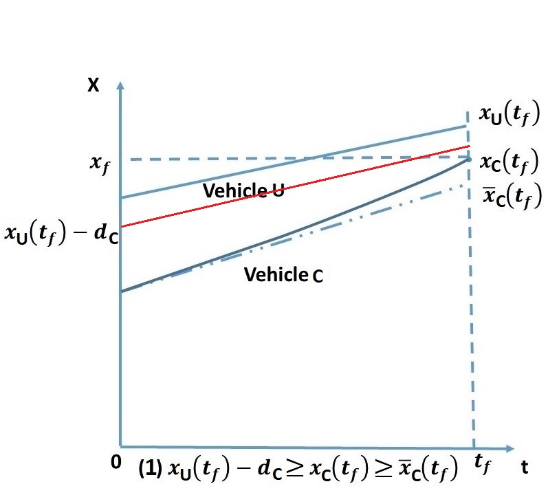
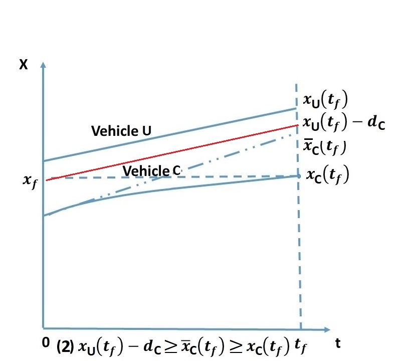
Figure 3: The three feasible cases for the optimal maneuver of vehicle $C$.

Theorem $4$ [Case 1 in Fig. 3]: If $\bar{x}_{C}(t_{f})<x_{C}(t_{f})<x_{U}(t_{f})-d_{C}$, then $u_{C}^{\ast}(t)\geq 0$ and $\eta_{5}^{\ast}(t)=0$.

Proof: The condition $x_{C}(t_{f})>\bar{x}_{C}(t_{f})$ implies that $u_{C}(t)\geq 0$ is a feasible solution of (18) since $u_{1}(t)<0$ for all $t\in[t_{0},t_{f}]$ cannot satisfy this condition. Suppose that there exists some $[t_{1},t_{2})\subset[0,t_{f}]$ in which the optimal solution satisfies $u_{C}^{\ast}(t)<0$. We will show that there exists another control which would lead to a lower cost than $u_{C}^{\ast}(t)$. First, we construct a control $u_{C}^{1}(t)$ such that $u_{C}^{1}(t)=u_{C}^{\ast}(t)\geq 0$ for $t\in[0,t_{1})\cup[t_{2},t_{f}]$, $u_{C}^{1}(t)=0$ for $t\in[t_{1},t_{2})$. It is clear that $u_{C}^{1}(t)$ will not violate the acceleration constraint (2). However, the terminal position constraint is violated. Therefore, we will construct $u_{C}^{2}(t)$, a variant of $u_{C}^{1}(t)$ as follows, and will show that $u_{C}^{2}(t)$ is feasible.

First, define

$$g_{C}(t)=x_{C}^{1}(t)+v_{C}^{1}(t)(t_{f}-t)$$ (21)

and note that $g_{C}(t)$ is continuous in $t$ since $x_{C}^{1}(t)$ and $v_{C}^{1}(t)$ are continuous. Because $g_{C}(0)=\bar{x}_{C}(t_{f})<x_{C}^{\ast}(t_{f})$ by assumption and $g_{C}(t_{f})=x_{C}^{1}(t_{f})\geq x_{C}^{\ast}(t_{f})$, there exists some $t_{m}\in[0,t_{f}]$ such that $g_{C}(t_{m})=x_{C}^{\ast}(t_{f})$. We can now construct $u_{C}^{2}(t)$ such that $u_{C}^{2}(t)=u_{C}^{1}(t)\geq 0$ for $t\in[0,t_{m})$, $u_{C}^{2}(t)=0$ for $t\in[t_{m},t_{f}]$. Observe that $x_{C}^{2}(t_{f})=g_{C}(t_{m})=x_{C}^{\ast}(t_{f})$. Moreover, based on its definition, it is obvious that it will not violate the acceleration constraint. Next, we show that the velocity constraint is also not violated. Suppose there exists some time $t_{n}$ such that $v_{C}^{1}(t_{n})=v_{C\text{max}}$ so that the trajectory may include an arc over which $v_{C}^{1}(t)=$$v_{C\text{max}}$. There are two cases:

(a) If $t_{n}\geq t_{m}$, we have $v_{C}^{1}(t_{m})\leq v_{C}^{1}(t_{n})$ because $u_{C}^{1}(t)\geq 0$. Based on the definition of $u_{C}^{1}(t)$, the maximal speed is $v_{C}^{1}(t_{m})$ and the velocity constraint is not violated.

(b) If $t_{n}<t_{m}$, we have $v_{C}^{1}(t_{m})>v_{C}^{1}(t_{n})$. Taking the time derivative of $g_{C}(t)$, we get $\dot{g}_{C}(t)=u_{C}^{1}(t)(t_{f}-t)\geq 0$. Therefore,

$$g_{C}(t_{n})<g_{C}(t_{m})=x_{C}^{\ast}(t_{f})$$ (22)

We then construct a control $u_{C}^{3}(t)$ such that $u_{C}^{3}(t)=u_{C}^{\ast}(t)\geq 0$ for $t\in[0,t_{1})\cup[t_{2},t_{n}]$, $u_{C}^{3}(t)=0$ for $t\in[t_{1},t_{2})\cup[t_{n},t_{f}]$. Note that $t_{n}\geq t_{1}$ because $v_{C}^{\ast}(t)\neq v_{C\text{max}}$ when $t<t_{1}$ based on the definition of $u_{C}^{\ast}(t)$. If $t_{1}<t_{n}<t_{2}$, we define $u_{C}^{3}(t)=0$ when $t>t_{1}$ as follows: $u_{C}^{3}(t)=u_{C}^{\ast}(t)\geq 0$, for $t\in[0,t_{1})$, $u_{C}^{3}(t)=0$, for $t\in[t_{1},t_{f}]$. From the construction of $u_{C}^{3}(t)$, we have $x_{C}^{3}(t_{n})=x_{C}^{1}(t_{n})$, $v_{C}^{3}(t_{n})=v_{C}^{1}(t_{n})$ so that (22) holds under $u_{1}^{3}(t)$, and $x_{C}^{3}(t_{f})=g_{C}(t_{n})$. Because $v_{C}^{3}(t)=v_{C\text{max}}$ for $t\in[t_{n},t_{f}]$ and $u_{C}^{3}(t)\geq u_{C}^{\ast}(t)$ for $t\in[0,t_{n})$, it is clear that $x_{C}^{3}(t)\geq x_{C}^{\ast}(t)$ for all $t\in[0,t_{f}]$. However, this contradicts (22) since $x_{C}^{3}(t_{f})=g_{C}(t_{n})<x_{C}^{\ast}(t_{f})$. We conclude that $t_{n}<t_{m}$ is not possible. In summary, we have proved that the speed constraint will not be violated under the control $u_{C}^{2}(t)$.

Next, we show that $u_{C}^{2}(t)$ will also not violate the safety constraint. Suppose that at time $t_{\sigma}\in[0,t_{f}]$, the safety constraint is active under control $u_{C}^{2}(t)$, i.e., $x_{C}^{2}(t_{\sigma})=x_{U}(t_{\sigma})-d_{C}$. Because $u_{C}^{2}(t)\geq 0$, based on Lemma $2$, it is straightforward to show that

$$x_{C}^{2}(t_{f})\geq x_{U}(t_{f})-d_{C}$$ (23)

Recall that, based on the definition of $u_{C}^{2}(t)$ and the condition that $x_{C}(t_{f})<x_{U}(t_{f})-d_{C}$, we have $x_{C}^{2}(t_{f})=g_{C}(t_{m})=x_{C}^{\ast}(t_{f})<x_{U}(t_{f})-d_{C}$ which contradicts with (23). Therefore, the safety constraint will never be activated.

We conclude that $u_{C}^{2}(t)$ is a feasible solution. Moreover, under $u_{C}^{2}(t)$ the cost is lower than that of $u_{C}^{\ast}(t)$ because $u_{C}^{2}(t)$ contains a segment with $u_{C}^{2}(t)=0$ that contributes zero cost in (18) relative to $u_{C}^{\ast}(t)$. Therefore, the optimal control $u_{C}^{\ast}(t)$ cannot contain any time interval with $u_{C}^{\ast}(t)<0$.

Finally, we use a similar argument as above to show that the safety constraint will be inactive under the optimal control $u_{C}^{\ast}(t)$, that is, $\eta_{5}^{\ast}(t)=0$. Assume that at time $t_{\eta}\in(0,t_{f}]$, $\eta_{5}^{\ast}(t_{\eta})>0$. Because the safety constraint is active at $t_{\eta}$ and is not violated at $t_{f}$, vehicle $C$ must have decelerated to relax the safety constraint. However, this violates the fact that $u_{C}^{\ast}(t)\geq 0$ as shown above. Therefore, we conclude that $\eta_{5}^{\ast}(t)=0$ for al $t\in[0,t_{f}]$. This completes the proof. $\blacksquare$

Theorem $5$ [Case 2 in Fig. 3]: If $x_{C}(t_{f})<\bar{x}_{C}(t_{f})<x_{U}(t_{f})-d_{C}$, then $u_{C}^{\ast}(t)\leq 0$ and $\eta_{5}^{\ast}(t)=0$.

Proof: The proof is similar to that of Theorem $4$ and is omitted. $\blacksquare$

Theorem $6$ [Case 3 in Fig. 3] If ${x}_{C}(t_{f})<x_{U}(t_{f})-d_{C}<\bar{x}_{C}(t_{f})$, then $u_{C}^{\ast}(t)\leq 0$.

Proof: The proof is similar to Theorem $4$. The only difference is in the way we prove that the constructed control $u_{C}^{2}(t)$ will not violate the safety constraint. Suppose that there exists some $[t_{1},t_{2})\subset[0,t_{f}]$ in which the optimal solution satisfies $u_{C}^{\ast}(t)>0$. First, we construct a control $u_{C}^{1}(t)$ such that $u_{C}^{1}(t)=u_{C}^{\ast}(t)\leq 0$ for $t\in[0,t_{1})\cup[t_{2},t_{f}]$, $u_{C}^{1}(t)=0$ for $t\in[t_{1},t_{2})$. It is clear that $x_{C}^{\ast}(t)\geq x_{C}^{1}(t)$, $v_{C}^{\ast}(t)\geq v_{C}^{1}(t)$, $t\in[0,t_{f}]$. Considering the safety constraint in (18), note that if $u_{C}^{\ast}(t)$ does not violate the safety constraint, then neither does $u_{C}^{1}(t)$.

Using $g_{C}(t)$ defined in (21), note that $g_{C}(0)=x_{C}^{1}(0)+v_{C}^{1}(0)t_{f}=\bar{x}_{C}(t_{f})$ and $g_{C}(t_{f})=x_{C}^{1}(t_{f})$. Since $x_{C}^{1}(t_{f})\leq x_{C}^{\ast}(t_{f})\leq\bar{x}_{C}(t_{f})$ and $g_{C}(t)$ is continuous, there exists $t_{m}\in(0,t_{f})$ such that $g_{C}(t_{m})=x_{C}^{\ast}(t_{f})$. Then, we construct $u_{C}^{2}(t)=u^{1}(t)\leq 0$ for $t\in[0,t_{m})$ and $u_{C}^{2}(t)=0$ for $[t_{m},t_{f}]$. Similar to the proof of Theorem $4$, $x_{C}^{2}(t_{f})=g_{C}(t_{m})=x_{C}^{\ast}(t_{f})$. Since $u_{C}^{2}(t)=u_{C}^{1}(t)$ for $t\in[0,t_{m})$, control $u_{C}^{2}(t)$ will not violate the safety constraint when $t\leq t_{m}$. For $t>t_{m}$, we have $u_{C}^{2}(t)=0$ and $x_{C}^{2}(t)$ is linear in $t$ with $v_{C}^{1}(t_{m})>0$. Moreover, $x_{C}^{1}(t_{m})<x_{U}(t_{m})-d_{C}$ and $x_{C}^{2}(t_{f})={x}_{C}^{\ast}(t_{f})<x_{U}(t_{f})-d_{C}$. We conclude that $u_{C}^{2}(t)$, $t\in[t_{m},t_{f}]$, will not violate the safety constraint because the upper bound of vehicle $C$’s safe position, $x_{U}(t)-d_{C}$, is also linear in $t$. Based on the definition of $u_{C}^{2}(t)$, it is obvious that it will not violate the acceleration constraint. We can then use the same argument as in the proof of Theorem $4$ to show that $v_{C}(t_{m})\geq v_{C\min}$. Therefore, $u_{C}^{2}(t)$ is a feasible solution. It is also obvious that the cost of $u_{C}^{2}(t)$ is lower than that of $u_{C}^{\ast}(t)$ because $u_{C}^{2}(t)$ contains a segment with $u_{C}^{2}(t)=0$. Therefore, the optimal control $u_{C}^{\ast}(t)$ cannot contain any time interval with $u_{C}^{\ast}(t)>0$. This completes the proof. $\blacksquare$

Based on Theorems 4,5, Cases 1,2 in Fig. 3 can be solved without the safety constraint in (18) since we have shown that $\eta_{5}^{\ast}(t)=0$. Therefore, the optimal control is the same as that derived for vehicles $1$ and $2$ in Theorems 2,3. This leaves only Case 3 to analyze. We proceed by first solving (18) without the safety constraint, so it reduces to the solution in Theorem 3, since we know that $u_{C}^{\ast}(t)\leq 0$. If a feasible optimal solution exists, then the problem is solved. Otherwise, we need to re-solve the problem in order to determine an optimal trajectory that includes at least one arc in which $x_{U}(0)+v_{U}(0)t-x_{C}^{\ast}(t)-d_{C}=0$.

Based on Lemma $2$, there exists a time $\tau_{1}\in(0,t_{f})$ that satisfies $v_{C}(\tau_{1})=v_{U}(0)$ and $x_{C}(\tau_{1})=x_{U}(0)+v_{U}(0)\tau_{1}-d_{C}\equiv a$ (it is easy to see that there is at most one such constrained arc, since $v_{C}(t)=v_{U}(0)$ as soon as this arc is entered.) We then split problem (18) into two subproblems as follows:

$$\min_{u_{C}(t)} \int_{0}^{\tau_{1}}\frac{1}{2}u_{C}^{2}(t)dt$$ (24)

s.t. $$\eqref{vehicle_dynamics},\text{ }\eqref{vehicle_constraint},\text{ }x_{C}(\tau_{1})=a,\text{ }v_{C}(\tau_{1})=v_{U}(\tau_{1}),\text{ }t\in[0,\tau_{1}]$$

$$\min_{u(t)}\int_{\tau_{1}}^{t_{f}}\frac{1}{2}u_{C}^{2}(t)dt\text{ s.t. }\eqref{vehicle_dynamics},\text{ }\eqref{vehicle_constraint},$$ (25)

$$\text{ }x_{C}(\tau_{1})=a,\text{ }v_{C}(\tau_{1})=v_{U}(\tau_{1}),\text{ }x_{C}(t_{f})=x_{cf},\text{ }t\in[\tau_{1},t_{f}]$$

where (24) has a fixed terminal time $\tau_{1}$ (to be determined), position $a$, and speed $v_{U}(0)$, while (25) has a fixed terminal time $t_{f}$ and position $x_{C,f}$ with given $x_{C}(\tau_{1})=a$.

Let us first solve (24). Since $u_{C}^{\ast}(t)\leq 0$ and the terminal speed is $v_{U}(0)$, only the acceleration constraint $u_{C\min}-u_{C}\leq 0$ can be active in $[0,\tau_{1}]$. Suppose that this constraint becomes active at time $\tau_{2}<\tau_{1}$. Since $u_{C\min}-u_{C}$ is independent of $t$, $x_{C}(t)$, and $v_{C}(t)$, it follows (see [20]) that there are no discontinuities in the Hamiltonian or the costates, i.e., $\lambda_{x}(\tau_{2}^{-})=\lambda_{x}(\tau_{2}^{+})$, $\lambda_{v}(\tau_{2}^{-})=\lambda_{v}(\tau_{2}^{+})$, $H(\tau_{2}^{-})=H(\tau_{2}^{+})$. It follows from $H(\tau_{2}^{-})-H(\tau_{2}^{+})=0$ and (19) that

$$[u_{C}^{\ast}(\tau_{2}^{-})-u_{C}^{\ast}(\tau_{2}^{+})][\frac{1}{2}(u_{C}^{\ast}(\tau_{2}^{-}))+\frac{1}{2}(u_{C}^{\ast}(\tau_{2}^{+}))+\lambda_{v}(\tau_{2}^{-})]=0$$

Therefore, either $u_{C}^{\ast}(\tau_{2}^{-})=u_{C}^{\ast}(\tau_{2}^{+})$ or $u_{C}^{\ast}(\tau_{2}^{-})=-{\lambda_{v}(\tau_{2}^{-})}$ based on (20). Either condition used in the above equation leads to the conclusion that $u_{C}^{\ast}(\tau_{2}^{-})=u_{C}^{\ast}(\tau_{2}^{+})$, i.e., $u_{C}^{\ast}(t)$ is continuous at $\tau_{2}$.

Let us now evaluate the objective function in (24) as a function of $\tau_{1}$ and $a$, denoting it by $J_{1}(\tau_{1},a)$, under optimal control. In view of (20), there are two cases.

(a) $u_{C}^{\ast}(t)=u_{C\text{min}}$ for $t\in[0,\tau_{2})$, $u_{C}^{\ast}(t)=-{\lambda_{v}(t)}$ for $t\in[\tau_{2},\tau_{1}]$. As in the proof of Theorem 2, the costate equations are $\dot{\lambda}_{v}(t)=-\lambda_{x}(t)$ and ${\dot{\lambda}}_{x}(t)=0$. Therefore, $\lambda_{v}(t)=ct-b$ where $b,c$ are to be determined. It follows that

$$u_{C}^{\ast}(t)=c(t-\tau_{2})+u_{C\text{min}}\text{, \ \ }t\in[\tau_{2},\tau_{1})$$ (26)

and the following boundary conditions hold:

$$v_{C}(\tau_{2}) =v_{C}(0)+u_{C\text{min}}\tau_{2}$$ (27)

$$v_{C}(\tau_{1}) =v_{U}(0)=v_{C}(\tau_{2})+\int_{\tau_{2}}^{\tau_{1}}[c(t-\tau_{2})+u_{C\text{min}}]dt$$

$$x_{C}(\tau_{2}) =x_{C}(0)+v_{C}(0)\tau_{2}+\frac{1}{2}u_{C\text{min}}\tau_{2}^{2}$$

$$x_{C}(\tau_{1}) =a=x_{C}(\tau_{2})+\int_{\tau_{2}}^{\tau_{1}}[\frac{c}{2}t^{2}+(u_{C\text{min}}-c\tau_{2})(t-\tau_{2})$$

$$-\frac{c}{2}\tau_{2}^{2}+v_{C}(0)+u_{C\text{min}}\tau_{2}]dt$$

Using (26) and (27) to eliminate $c$ and $\tau_{2}$ and then evaluate $J_{1}(\tau_{1},a)$ in (24) after some algebra yields:

$$J_{1}(\tau_{1},a)= \frac{1}{2}u_{\text{Cmin}}(2v_{U}(0)-2v_{C}(0)-u_{\text{Cmin}}\tau_{1})$$ (28)

$$+\dfrac{2(v_{U}(0)-v_{C}(0)-u_{\text{Cmin}}\tau_{1})^{3}}{9(a-x_{C}(0)-v_{C}(0)\tau_{1}-0.5u_{\text{Cmin}}\tau_{1}^{2})}$$

(b) $u_{C}^{\ast}(t)=-{\lambda_{v}(t)}$ for $t\in[0,\tau_{2})$, $u_{C}^{\ast}(t)=u_{C\text{min}}$ for $t\in[\tau_{2},\tau_{1}]$. Proceeding as above, we get

$$v_{C}(\tau_{2}) =v_{C}(0)+\int_{0}^{\tau_{2}}[c(\tau_{2}-t)+u_{C\text{min}}]dt$$ (29)

$$v_{C}(\tau_{1}) =v_{U}(0)=v_{C}(\tau_{2})+(\tau_{1}-\tau_{2})u_{C\text{min}}$$

$$x_{C}(\tau_{2}) =x_{C}(0)+\int_{0}^{\tau_{2}}[v_{C}(0)+\frac{c}{2}t^{2}+u_{C\text{min}}t]dt$$

$$x_{C}(\tau_{1}) =a=x_{C}(\tau_{2})+\int_{\tau_{2}}^{\tau_{1}}[v_{C}(\tau_{2})+u_{C\text{min}}(t-\tau_{2})]dt$$

and, after some calculations, we obtain $J_{1}(\tau_{1},a)$ in (24):

$$J_{1}(\tau_{1},a)=\frac{1}{2}u_{\text{Cmin}}(2v_{U}(0)-2v_{C}(0)-u_{\text{Cmin}}\tau_{1})$$ (30)

$$-\dfrac{2(v_{U}(0)-v_{C}(0)-u_{\text{Cmin}}\tau_{1})^{3}}{9(a-x_{C}(0)-v_{U}\tau_{1}+0.5u_{\text{Cmin}}\tau_{1}^{2})}$$

Proceeding to the second subproblem (25), note that the control at the entry point of the constrained arc at time $\tau_{1}$ is no longer guaranteed to be continuous. This problem is of the same form as the optimal control problem for vehicle 2 in (10) whose solution is given in Theorem 3, except that initial conditions now apply at time $\tau_{1}$ as given in (25). Proceeding exactly as before, we can obtain the cost $J_{2}(\tau_{1},a)$ under optimal control. Adding the two costs, we obtain $J_{C}(\tau_{1},a)=J_{1}(\tau_{1},a)+J_{2}(\tau_{1},a)$ in (18). This results in a simple nonlinear programming problem whose solution $(\tau_{1}^{\ast},a^{\ast})$ results from setting $\dfrac{\partial J_{C}(\tau_{1},a)}{\partial\tau_{1}}=0$ and $\dfrac{\partial J_{C}(\tau_{1},a)}{\partial a}=0$. Finally, the optimal control is the one corresponding to $(\tau_{1}^{\ast},a^{\ast})$.

Based on our analysis, we find that Case 3 is the only one where the safety constraint may become active. This provides an option to the vehicle $C$ controller: if Case 3 applies, the maneuver may either be implemented or it may be delayed until the conditions change to either one of Cases 1,2 so as avoid the more complex situation that arises through (24),(25).

IV Simulation Results

We provide simulation results illustrating the time and energy-optimal optimal maneuver controller we have derived and compare its performance to a baseline of human-driven vehicles. In what follows, we set the minimal and maximal vehicle speeds to $1m/s$ and $33m/s$ respectively and the maximal acceleration and deceleration to $3.3m/s^{2}$ and $-7m/s^{2}$ respectively. The aggressiveness coefficients $\alpha_{i},i=1,2,C$ in (4) are all set to $\alpha_{i}=0.5$.

Case 1 in Fig. 3. We set $x_{1}(t_{0})=90m$, $v_{1}(t_{0})=13m/s$, $x_{U}(t_{0})=100m$, $v_{U}(t_{0})=9m/s$, $x_{2}(t_{0})=50m$, $v_{2}(t_{0})=18m/s$ and $x_{C}(t_{0})=13m$, $v_{C}(t_{0})=10m/s$. Solving (4), we get $t_{f}=28.14s$ and after solving (5), we obtain $x_{1}(t_{f})=455.8m$, $x_{C}(t_{f})=303.24m$ and $x_{2}(t_{f})=273.24m$. Figs. 4-5 show the optimal trajectories of all controllable vehicles. In Fig. 4, vehicle $1$ is cruising with a constant velocity which contributes a zero value to the cost in (6), while the velocity of vehicle $2$ decreases to create space for vehicle $C$ to change lanes. The optimal trajectory of vehicle $C$ in Fig. 5 is obtained without considering the safety constraint because of Theorem $4$. Vehicle $C$ keeps on accelerating and the safety distance constraint is never violated.

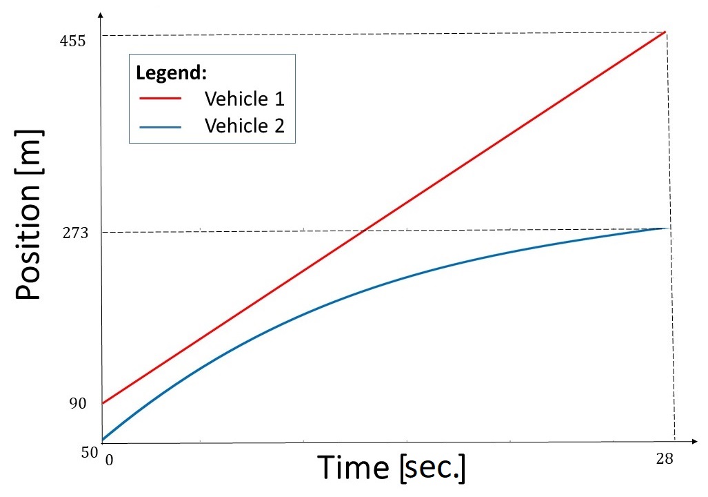
Figure 4: Optimal Position trajectories of vehicle $1$ and $2$ in case ($1$) of Fig. 3.

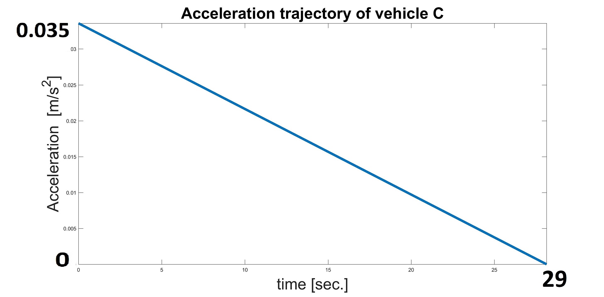
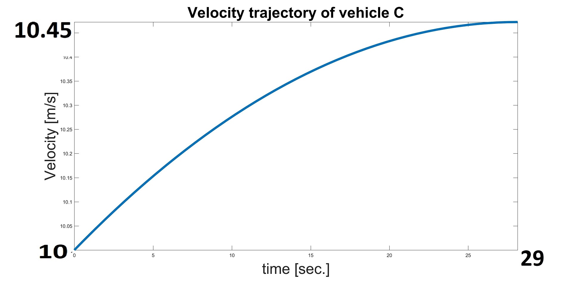
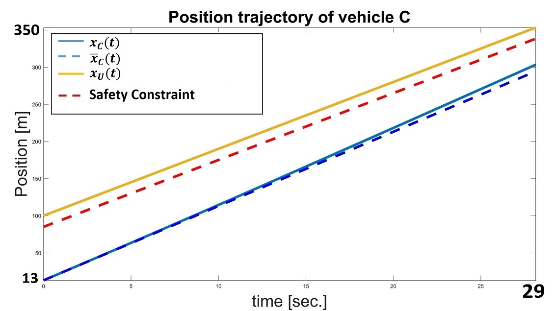
Figure 5: Optimal trajectories of vehicle $C$ in case ($1$) of Fig. 3.

Case 2 in Fig. 3. We set $x_{1}(0)=70m$, $v_{1}(0)=13m/s$, $x_{2}(0)=30m$, $v_{2}(0)=18m/s$, $x_{C}(0)=13m$, $v_{C}(0)=12m/s$, $x_{U}(0)=80m$, $v_{U}(0)=10m/s$. Solving (4) and (5), we get $t_{f}=21.4s$ and $x_{1}(t_{f})=348.37m$, $x_{2}(t_{f})=214.13m$, $x_{C}(t_{f})=244.13m$. Figure 6 shows the optimal trajectories of vehicles $1$,$2$ in which $1$ is cruising with a constant speed and the associated energy cost is zero, while the velocity of vehicle $2$ decreases. Figure 7 shows the optimal trajectory of vehicle $C$ which, once again, is obtained without considering the safety constraint based on Theorem $5$. Vehicle $C$ decelerates to ensure it satisfies its terminal position while the safety constraint is never violated.

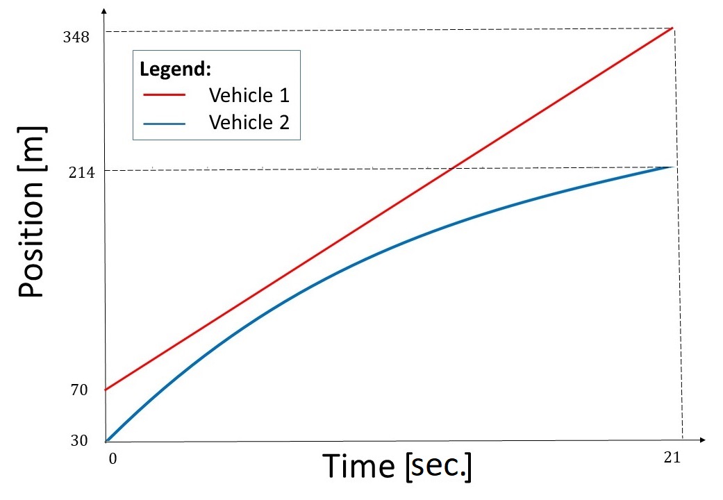
Figure 6: Optimal Position trajectories of vehicle $1$ and $2$ in case ($2$) of Fig. 3.

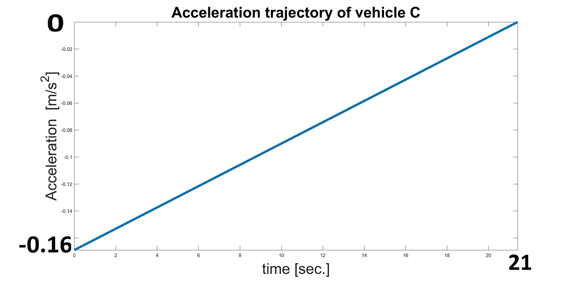
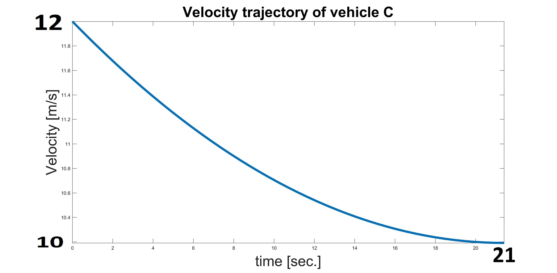
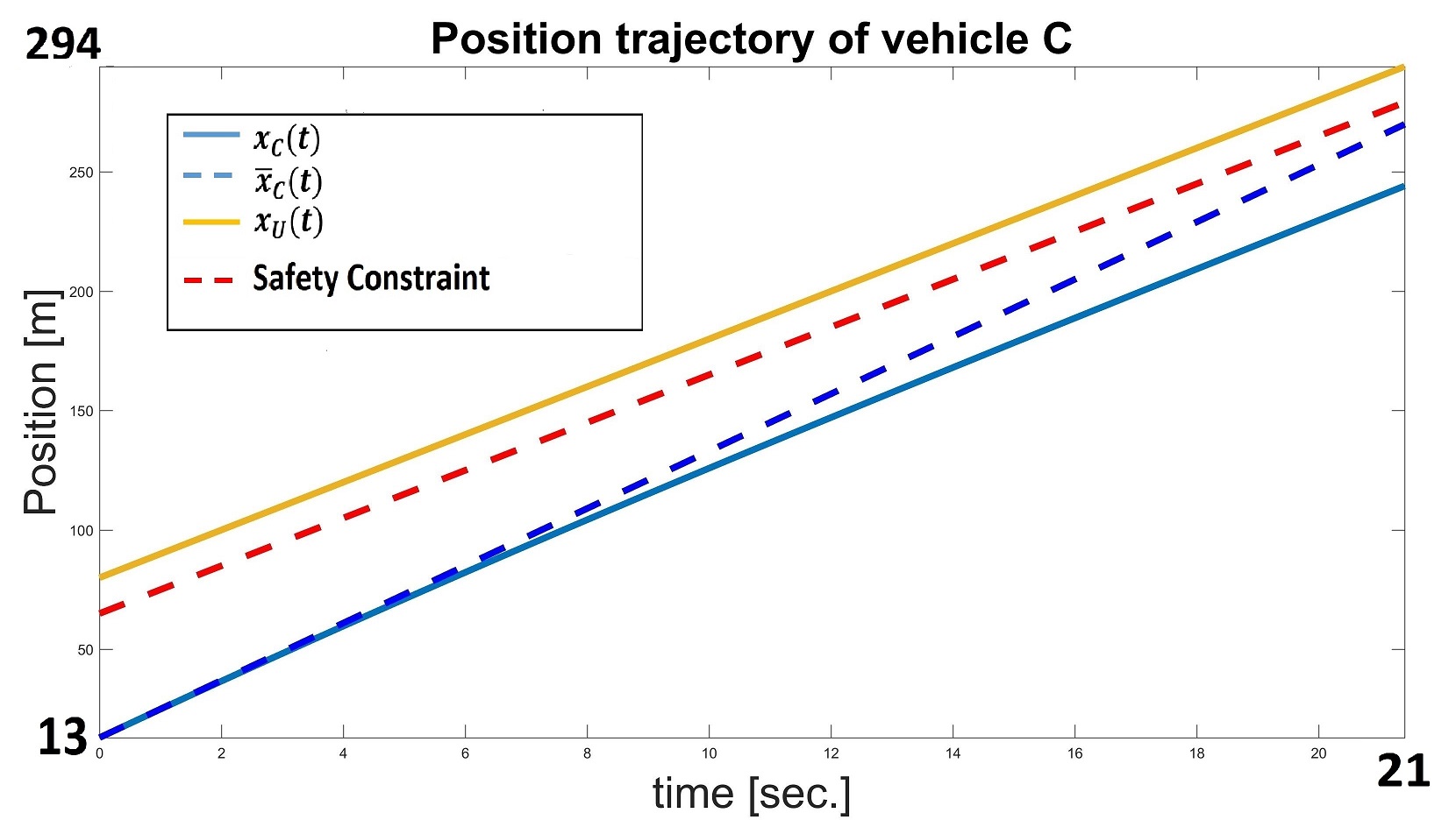
Figure 7: Optimal trajectories of vehicle $C$ in case ($2$) of Fig. 3.

Case 3 in Fig. 3. We set $x_{1}(0)=40m$, $v_{1}(0)=11m/s$, $x_{U}(0)=40m$, $v_{U}(0)=8m/s$ $x_{2}(0)=10m$, $v_{2}(0)=23m/s$, $x_{C}(0)=13m$, $v_{C}(0)=19m/s$. Solving (4) and (5), we get $t_{f}=14.49s$ and $x_{1}(t_{f})=199.37m$, $x_{2}(t_{f})=75m$, $x_{C}(t_{f})=105.9m$. The optimal trajectories of vehicles $1$,$2$ are shown in Fig. 8. In this case, vehicle $1$ accelerates and vehicle $2$ decelerates in order to create space for vehicle $C$. For vehicle $C$, we first solve the optimal control problem (18) without considering the safety constraint and find that it actually becomes active. Therefore, we proceed with the two subproblems (24) and (25) to derive the true optimal trajectories. We obtained $a^{\ast}=43m$ and $\tau_{1}^{\ast}=3.2s$, and Fig. 9 shows the optimal trajectory of vehicle $C$. Observe that $C$ decelerates over the maneuver and the safety distance constraint is active at $\tau_{1}^{\ast}=3.2s$ when there is a jump in the acceleration trajectory. Following that, vehicle $C$ continues decelerating until it reaches its terminal position.

Comparison of optimal maneuver control and human-driven vehicles. We use standard car-following models in the commercial SUMO simulator to simulate a lane change maneuver implemented by human-driven vehicles with the requirement that vehicle $C$ changes lanes between vehicles $1$ and $2$. We considered all cases in Fig. 3 with both CAVs and human-driven vehicles sharing the same initial states as shown in Table I.

TABLE I: Initial states of vehicles

	$x_{1}(0)[m]$	$v_{1}(0)[m/s]$	$x_{2}(0)[m]$	$v_{2}(0)[m/s]$	$x_{C}(0)[m]$	$v_{C}(0)[m/s]$	$x_{U}(0)[m]$	$v_{U}(0)[m/s]$	$d_{C}[m]$
(1)	95	13	0	18	13	10	120	9	30
(2)	120	13	30	18	13	16	100	10	30
(3)	100	11	10	23	213	19	290	8	30

The associated energy consumption is shown in Table II and provides evidence of savings in the range $43-59\%$ over all three cases.

TABLE II: ENERGY COMPARISON: CAVs vs HUMAN-DRIVEN VEHICLES

	CAVs	Human-driven Vehicles	Improvement
(1)	6.8	16.4	59%
(2)	23.0	46.0	50%
(3)	59.5	103.5	43%

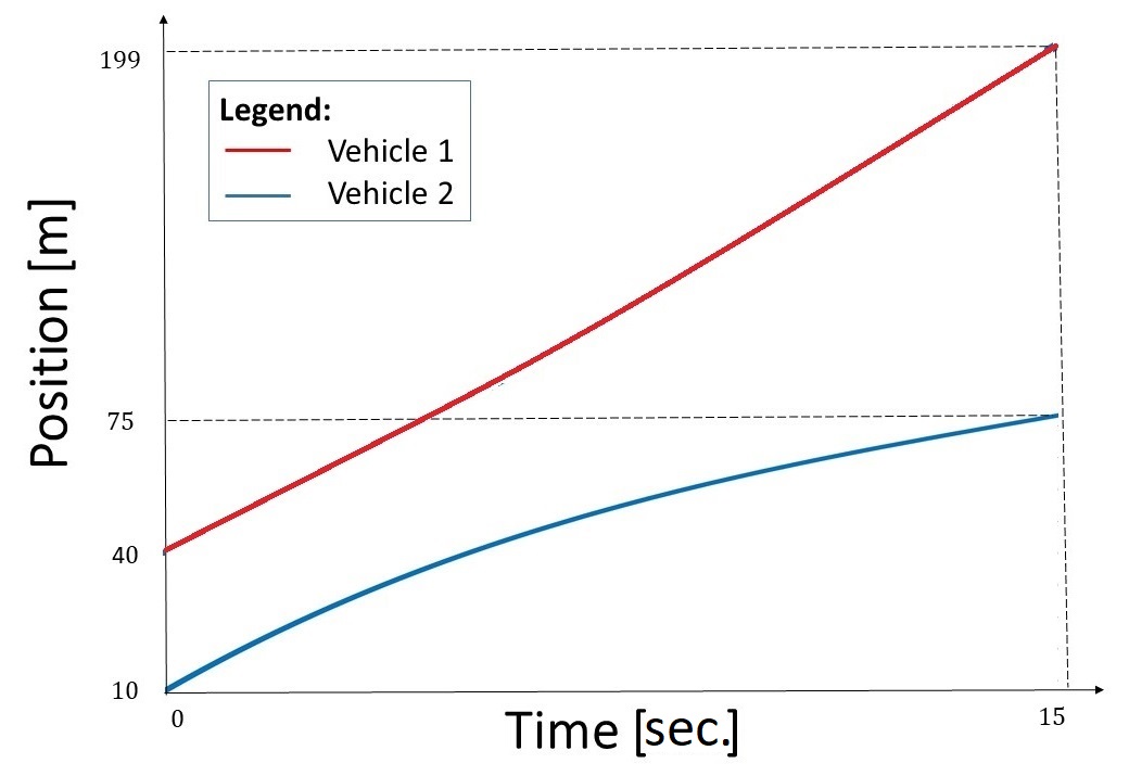
Figure 8: Optimal Position trajectories of vehicle $1$ and $2$ in case ($3$) of Fig. 3.

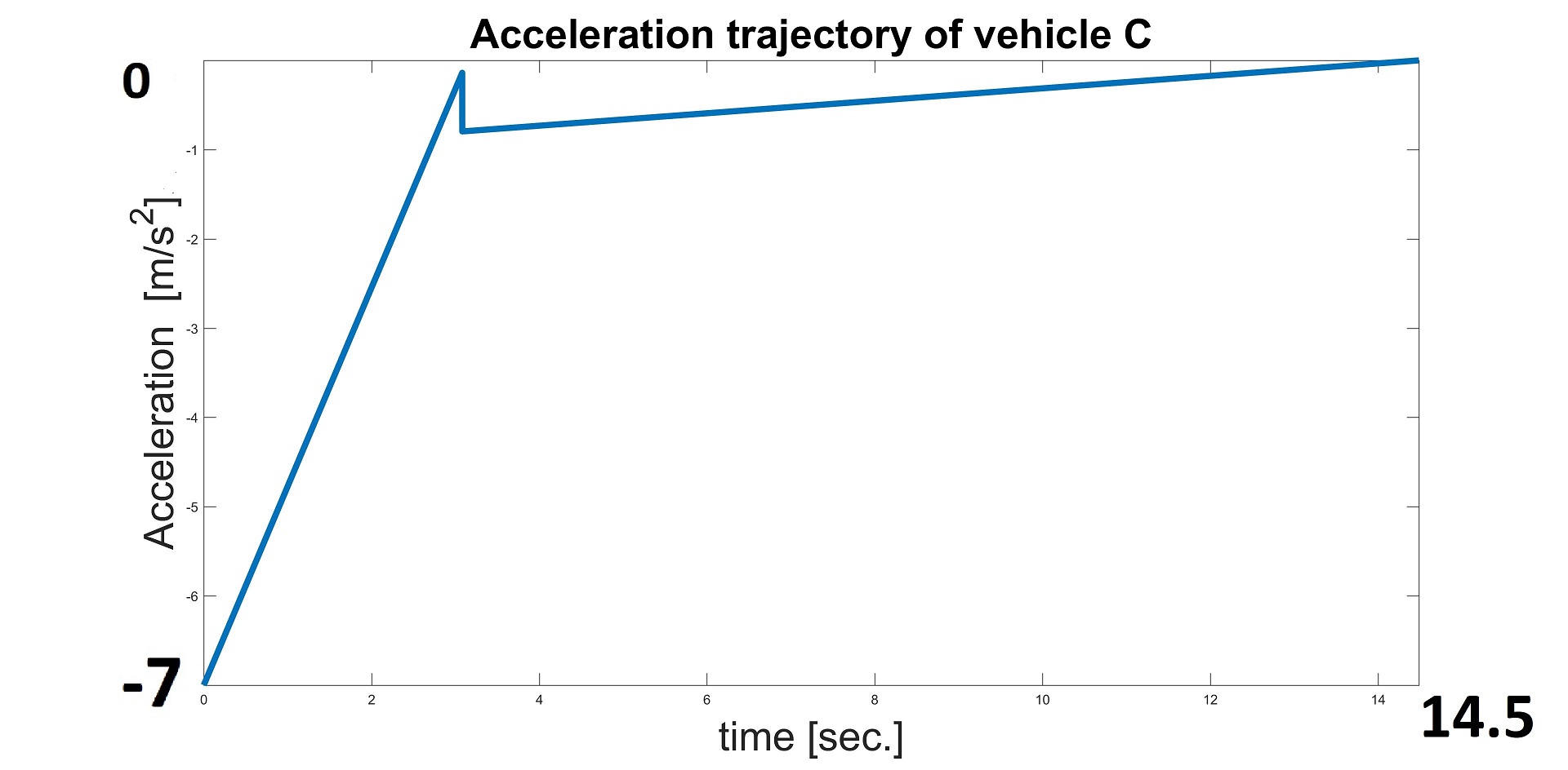
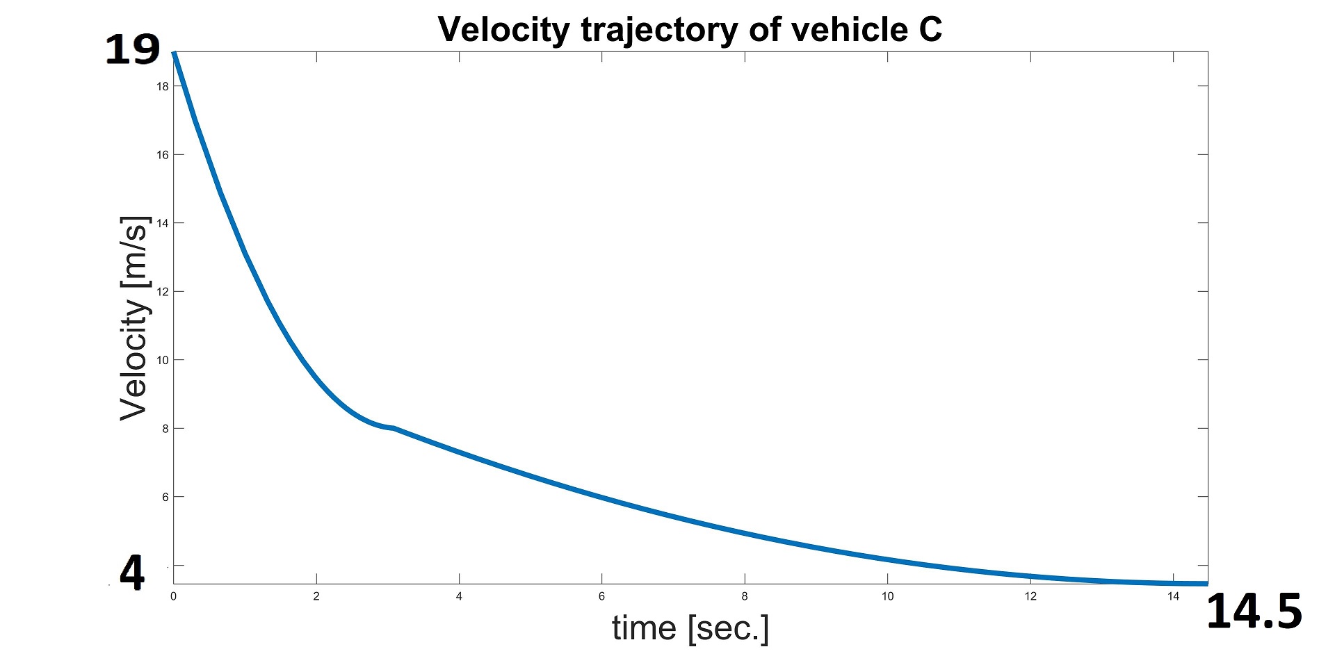
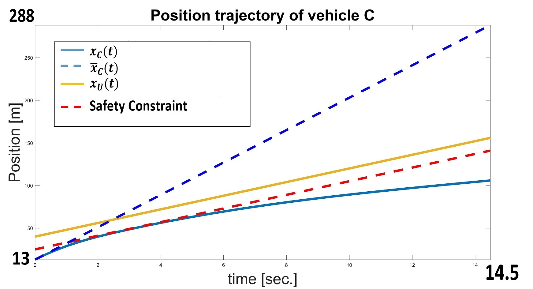
Figure 9: Optimal trajectories of vehicle $C$ in case ($3$) of Fig. 3.

V Conclusion and Future Work

We used an optimal control framework to derive time and energy-optimal policies for a CAV cooperating with neighboring CAVs to implement a highway lane change maneuver. We optimize the maneuver time and subsequently minimize the associated energy consumption of all cooperating vehicles in this maneuver. Our solution is limited to the first step of the complete maneuver, i.e., all three cooperating vehicles adjust their positions before the lane-changing vehicle makes the lane shift. Our ongoing work aims to complete this step. In addition, we plan to incorporate a “comfort” factor in the problem by minimizing any resulting jerk and adopt a more general velocity-varying safety distance constraint.

References

- [1] P. Varaiya, “Smart cars on smart roads: problems of control,” IEEE Trans. on Automatic Control, vol. 38, no. 2, pp. 195–207, 1993.
- [2] D. Zhao, X. Huang, H. Peng, H. Lam, and D. J. LeBlanc, “Accelerated evaluation of automated vehicles in car-following maneuvers,” IEEE Trans. on Intelligent Transportation Systems, vol. 19, no. 3, pp. 733–744, 2018.
- [3] M. Wang, W. Daamen, S. P. Hoogendoorn, and B. van Arem, “Cooperative car-following control: Distributed algorithm and impact on moving jam features,” IEEE Trans. on Intelligent Transportation Systems, vol. 17, no. 5, pp. 1459–1471, 2016.
- [4] M. Wang, S. P. Hoogendoorn, W. Daamen, B. van Arem, and R. Happee, “Game theoretic approach for predictive lane-changing and car-following control,” Transportation Research Part C: Emerging Technologies, vol. 58, pp. 73–92, 2015.
- [5] J. Nilsson, M. Brännström, E. Coelingh, and J. Fredriksson, “Longitudinal and lateral control for automated lane change maneuvers,” Proc. of 2015 American Control Conf., pp. 1399–1404, 2015.
- [6] C. Bax, P. Leroy, and M. P. Hagenzieker, “Road safety knowledge and policy: A historical institutional analysis of the Netherlands,” Transportation Research part F: Traffic Psychology and Behaviour, vol. 25, pp. 127–136, 2014.
- [7] F. You, R. Zhang, G. Lie, H. Wang, H. Wen, and J. Xu, “Trajectory planning and tracking control for autonomous lane change maneuver based on the cooperative vehicle infrastructure system,” Expert Systems with Applications, vol. 42, no. 14, pp. 5932–5946, 2015.
- [8] M. Werling, J. Ziegler, S. Kammel, and S. Thrun, “Optimal trajectory generation for dynamic street scenarios in a frenet frame,” Proc. of 2010 IEEE Intl. Conf. on Robotics and Automation, pp. 987–993, 2010.
- [9] D. Bevly, X. Cao, M. Gordon, G. Ozbilgin, D. Kari, B. Nelson, J. Woodruff, M. Barth, C. Murray, A. Kurt et al., “Lane change and merge maneuvers for connected and automated vehicles: A survey,” IEEE Trans. on Intelligent Vehicles, vol. 1, no. 1, pp. 105–120, 2016.
- [10] J. Nilsson, M. Brännström, E. Coelingh, and J. Fredriksson, “Lane change maneuvers for automated vehicles,” IEEE Trans. on Intelligent Transportation Systems, vol. 18, no. 5, pp. 1087–1096, 2017.
- [11] Y. Luo, Y. Xiang, K. Cao, and K. Li, “A dynamic automated lane change maneuver based on vehicle-to-vehicle communication,” Transportation Research Part C: Emerging Technologies, vol. 62, pp. 87–102, 2016.
- [12] H. N. Mahjoub, A. Tahmasbi-Sarvestani, H. Kazemi, and Y. P. Fallah, “A learning-based framework for two-dimensional vehicle maneuver prediction over v2v networks,” Proc. of 15th IEEE Intl. Conf. on Dependable, Autonomic and Secure Computing, pp. 156–163, 2017.
- [13] H. Kazemi, H. N. Mahjoub, A. Tahmasbi-Sarvestani, and Y. P. Fallah, “A learning-based stochastic MPC design for cooperative adaptive cruise control to handle interfering vehicles,” IEEE Trans. on Intelligent Vehicles, vol. 3, no. 3, pp. 266–275, 2018.
- [14] M. A. S. Kamal, M. Mukai, J. Murata, and T. Kawabe, “Model predictive control of vehicles on urban roads for improved fuel economy,” IEEE Trans. on Control Systems Technology, vol. 21, no. 3, pp. 831–841, 2013.
- [15] A. Katriniok, J. P. Maschuw, F. Christen, L. Eckstein, and D. Abel, “Optimal vehicle dynamics control for combined longitudinal and lateral autonomous vehicle guidance,” Proc. of 2013 Control Conf., pp. 974–979, 2013.
- [16] S. Lam and J. Katupitiya, “Cooperative autonomous platoon maneuvers on highways,” Proc. of 2013 IEEE/ASME Intl. Conf. on Advanced Intelligent Mechatronics, pp. 1152–1157, 2013.
- [17] B. Li, Y. Zhang, Y. Ge, Z. Shao, and P. Li, “Optimal control-based online motion planning for cooperative lane changes of connected and automated vehicles,” Proc. of 2017 IEEE/RSJ Intl. Conf. on Intelligent Robots and Systems, pp. 3689–3694, 2017.
- [18] K. Vogel, “A comparison of headway and time to collision as safety indicators,” Accident Analysis & Prevention, vol. 35, no. 3, pp. 427–433, 2003.
- [19] X. Meng and C. G. Cassandras, “Optimal control of autonomous vehicles for non-stop signalized intersection crossing,” Proc. of 57th IEEE Conf. on Decision and Control, pp. 6988–6993, 2018.
- [20] A. E. Bryson, Applied optimal control: optimization, estimation and control. Routledge, 2018.