Matrix-free multigrid solvers
for phase-field fracture problems

Abstract

In this work, we present a framework for the matrix-free solution to a monolithic quasi-static phase-field fracture model with geometric multigrid methods. Using a standard matrix based approach within the Finite Element Method requires lots of memory, which eventually becomes a serious bottleneck. A matrix-free approach overcomes this problems and greatly reduces the amount of required memory, allowing to solve larger problems on available hardware. One key challenge is concerned with the crack irreversibility for which a primal-dual active set method is employed. Here, the active set values of fine meshes must be available on coarser levels of the multigrid algorithm. The developed multigrid method provides a preconditioner for a generalized minimal residual (GMRES) solver. This method is used for solving the linear equations inside Newton’s method for treating the overall nonlinear-monolithic discrete displacement/phase-field formulation. Several numerical examples demonstrate the performance and robustness of our solution technology. Mesh refinement studies, variations in the phase-field regularization parameter, iterations numbers of the linear and nonlinear solvers, and some parallel performances are conducted to substantiate the efficiency of the proposed solver for single fractures, multiple pressurized fractures, and a L-shaped panel test in three dimensions.

Keywords: phase-field fracture propagation; matrix-free; geometric multigrid; primal-dual active set

1 Introduction

Predicting fracture growth can be of big interest in a variety of fields, such as manufacturing processes, engineering sciences, and medical applications. However, fracture propagation poses several challenges for numerical methods. A main problem is the fact, that cracks are usually lower-dimensional phenomena. For example, fractures in a sheet of glass are, most often, just thin lines. This makes it very difficult for standard numerical methods, like the Finite Element Method (FEM) to represent such kind of discontinuities. Another challenge is the irreversibility property, i.e. a fracture should not be able to heal itself, which introduces time-dependent constraints on the solution. More difficulties are related to fracture nucleation, branching, and fracture networks with curve-linear, complex, crack patterns.

Methods like generalized/extended FEM (GFEM/XFEM) try to overcome these fallacies of standard FEM by enriching the solution space with discontinuous functions. This allows the representation of sharper objects like cracks, see e.g. [11, 54]. A short overview of various methods is compiled in [70].

We now focus on a variational phase-field based approach, which was first introduced for fractures in [16] based on the fracture model presented in [25]. Therein, Griffith’s original model for brittle fractures [29] is rewritten by means of an energy minimization problem. This numerical approximation introduces an additional scalar-valued indicator variable representing the fracture. It is then computed as the minimizer of the total energy functional, together with the unknown solid displacement. Specifically therein, the continuous model is approximated using elliptic Ambrosio-Tortorelli functionals, see [4]. Such an approximation yields a smooth representation of the originally sharp crack. Thus, the solution does no longer jump from broken to unbroken parts, but provides a smoothed transition between them. The approximation quality is given by the phase-field regularization parameter $\varepsilon$. Roughly speaking, it determines the size of the diffusive zone around the fracture, see Figure 1 for an illustration.

This smoothing effect could be seen as a disadvantage of phase-field methods, as it is no longer possible to accurately localize the fracture. Indeed, fracture width computations [51] and posing interface conditions on the fracture boundary are challenging [60] with no final answer to date. On the other hand, it comes with some benefits: the problem is reduced to find the minimizers of a nonlinear energy functional, which is a common procedure in engineering and applied mathematics. Thus, it is possible to use well-known Galerkin techniques, making it easier to find suitable software to assist with the implementation. Furthermore, the fracture is entirely represented using an additional variable. In particular, the mesh is fixed and does not need to be updated when the fracture propagates, as it is the case for methods like XFEM.

The phase-field fracture (PFF) model can be enhanced to include, for instance, pressure-driven cracks; see, e.g, [59, 58, 52, 61, 62, 35, 73, 76, 21, 66]. Furthermore, thermodynamically consistent schemes have been developed in [56, 57]. Therein, the elastic energy is split into tensile and compressive parts. Other splitting strategies exists, e.g. [6] based on a deviatoric split, or a hybrid strategy as presented in [3]. The latter also contains a nice comparison of the different splitting techniques.

The most challenging part is related to the nonlinear equations and the irreversibility condition, which appears in terms of a variational inequality. For treating the irreversibility constraint, several approaches (simple penalization, augmented Lagrangian techniques, or a strain-history field) have been proposed in the literature. In this work, we adopt a primal-dual active set method [40, 43] that can be identified as a semi-smooth Newton method [40] and was first applied to phase-field fracture in [36]. With regard to the nonlinearities in the governing equations for displacements and phase-field two main approaches can be distinguished: staggered approaches [15, 20, 56] and monolithic methods [27, 71, 72].

Typically, the nonlinear solvers reduce the problem to the repeated solution of linear systems of equations. Krylov-subspace based solvers like Conjugate Gradients (CG) or Generalized Minimal Residual (GMRES) [64] have been proven to be very effective methods for solving such large sparse linear systems, if provided with a reasonable preconditioner. Different possibilities to precondition the PFF problem are shown in [23].

A powerful class of solvers/preconditioners that is known to work for many different types of problems are multigrid methods. These methods smooth the iteration error on the fine grid and correct the iterate by a course-grid correction in a two-grid setting, whereas a recurrent applications on a sequence of grids lead to a multigrid procedure; see [32, 18]. Multigrid methods have been successfully applied to a wide range of related problems, see e.g. [44, 45, 33, 41, 42, 10, 13, 63, 38, 28, 46]. Algebraic multigrid methods provided by Trilinos [39, 26] have been applied to phase-field fracture in [37], yielding a scalable parallel solution scheme; see also [67, 30, 19] for algebraic multigrid method and their parallelization.

When attempting to solve larger and larger problems, memory soon becomes the limiting factor. To overcome this, matrix-free methods have been developed. Instead of assembling and storing the discrete Jacobian, as it is usually done, the necessary information is computed on-the-fly. This drastically reduces the amount of memory required, but may increase the computational cost. Hence, a clever implementation is needed to keep up with standard matrix-based methods. In this work, we rely on the FEM library deal.II [2], which readily includes such an implementation [48, 49].

As indicated in our previous overviews, the main aims of this paper are two-fold:

• Development of a geometric multigrid preconditioner for the GMRES iterations inside Newton’s method;

• A matrix-free implementation of the geometric multigrid method.

Here, one focus is on quantities that are given naturally on the finest grid and which may also be required on the coarser levels of the multigrid algorithm, e.g. the current linearization point or the Active-Set. We will present strategies to handle those problems with relative ease. Indeed, the FEM library deal.II has gone to great lengths in providing a rich and flexible interface for the implementation of such sophisticated methods.

The outline of this paper is as follows. In Section 2, we will describe the governing equations of phase-field fractures and clarify some of the notation used. Furthermore, we briefly describe some details on the general discretization scheme used. In Section 3, we discuss our approach for the solution of the phase-field problem. This includes the non-linear solver (Active-Set) and the linear solver (geometric Multigrid). The main part of this work is presented in Section 4, which is devoted to the matrix-free realization of this solution approach. Finally, we present our findings and numerical results for various test cases in Section 5.

2 Problem Description

In this section, we introduce the basic notation and the underlying equations. In the following, let $D\subset\mathbb{R}^{d},d=2,3$ the total domain wherein $\mathcal{C}\subset\mathbb{R}^{d-1}$ denotes the fracture and $\Omega\subset\mathbb{R}^{d}$ is the intact domain. We assume (possibly time-dependent non-homogeneous) Dirichlet conditions on the outer boundary $\partial D$.

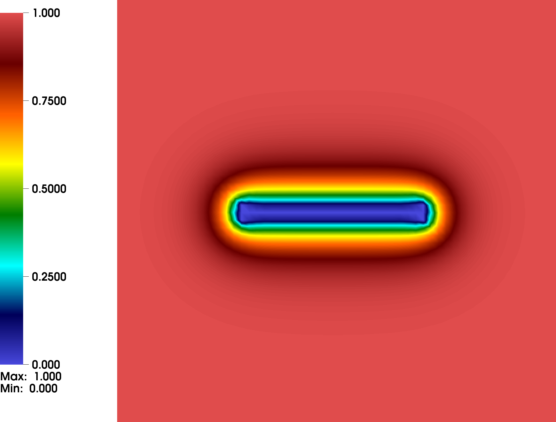
Figure 1: Illustration of the Notation: sharp fracture $\mathcal{C}$ and phase-field approximation $\Omega_{F}$.

In the phase-field approach, the one-dimensional fracture $\mathcal{C}$ is approximated by $\Omega_{F}\subset\mathbb{R}^{d}$ with the help of an elliptic (Ambrosio-Tortorelli) functional [4, 5]. Using the phase-field variable $\varphi$ (introduced in Section 2), $\Omega_{F}$ can be defined as

$$\Omega_{F}:=\{x\in\mathbb{R}^{d}|\;\varphi(x)<1\}.$$ (1)

The lower-dimensional fracture $\mathcal{C}$ and its phase-field approximation $\Omega_{F}$ are visualized in Figure 1. The width of the phase-field fracture is determined by $\varepsilon$. For fracture formulations posed in a variational setting, this has been first proposed in [16]. The inner fracture boundary is denoted by the smeared $\varepsilon$-dependent boundary $\partial\Omega_{F}$. We note that the precise location of $\partial\Omega_{F}$ is of no importance in this work (in contrast to e.g., [60]). The reader is referred to Figure 1 for an illustration of the notation. Finally, we denote the $L^{2}$ scalar product with $(a,b):=(a,b)_{D}:=\int_{D}a\cdot b\ dx$. For tensor-valued functions $A,B$, we use $(A,B):=(A,B)_{D}:=\int_{D}A:B\ dx$.

2.1 Quasi-static phase-field for brittle fracture

We briefly recapitulate the ingredients for a phase-field model for solid mechanics and pressurized fractures in brittle materials. Such a model is based on the variational/phase-field fracture approach of [25, 16]. Thermodynamically-consistent phase-field techniques using a stress-split into tension and compression have been proposed in [6] and [57].

The previous formulations start with an energy functional $E(u,\varphi)$ which is minimized with respect to the unknown solution variables $u:D\to\mathbb{R}^{d}$ (displacements) and a smoothed scalar-valued phase-field function $\varphi:D\to[0,1]$. The latter one varies in the zone of size $\varepsilon$ from $0$ (fracture) to $1$ (intact material). The first-order necessary condition are the Euler-Lagrange equations, which are obtained by differentiation with respect to the two unknowns $u$ and $\varphi$. Adding a pressure $p:D\to\mathbb{R}$ to the Euler-Lagrange equations that acts on the fracture boundary has been formulated and mathematically analyzed in [61, 62] for staggered and monolithic approaches, respectively. In all the previous fracture models, the physics of the underlying problem ask to enforce a crack irreversibility condition (the crack can never heal) that is an inequality condition in time:

$$\partial_{t}\varphi\leq 0.$$ (2)

Consequently, modeling of fracture evolution problems leads to a variational inequality system, that is always, due to this constraint, quasi-stationary or time-dependent. The resulting variational formulation is stated in an incremental (i.e., time-discretized) formulation in which the continuous irreversibility constraint is approximated by

$$\varphi\leq\varphi^{old}.$$

Here, $\varphi^{old}$ will later denote the previous time step solution and $\varphi$ the current solution. Let $V:=H^{1}_{0}(D)$ and

$$W_{in}:=\{w\in H^{1}(D)|\,w\leq\varphi^{old}\leq 1\text{ a.e. on }D\}$$ (3)

be the function spaces we work with here; and for later purposes we also need $W:=H^{1}(D)$. The Euler-Lagrange system for pressurized phase-field fractures reads [62]:

Problem 2.1.

Let $p\in L^{\infty}(D)$ be given. Find vector-valued displacements and a scalar-valued phase-field variable $\{u,\varphi\}:=\{u^{n},\varphi^{n}\}\in\{u_{D}+V\}\times W_{in}$ such that:

$$\left(g_{\kappa}(\varphi)\sigma^{+}(u),e(w)\right)+\left(\sigma^{-}(u),e(w)\right)+\left(\varphi^{2}p,\mbox{div }w\right)=0\quad \forall w\in V,$$

$$\frac{1}{2}\left(\partial_{\varphi}g_{\kappa}(\varphi)E_{s}^{+}(e(u)),\psi-\varphi\right)+2(\varphi\ p\ \mbox{div }u,\psi-\varphi)$$

$$+G_{c}\left(-\frac{1}{\varepsilon}(1-\varphi,\psi-\varphi)+\varepsilon\left(\nabla\varphi,\nabla(\psi-\varphi)\right)\right)\geq 0\quad \forall\psi\in W\cap L^{\infty}(D),$$

at each incremental step $n=1,2,3,\ldots$.

The elastic energy is denoted by

$$E_{s}(e):=\frac{1}{2}\lambda\mbox{tr}(e)^{2}+\mu(e,e)$$

with resulting stress tensor

$$\sigma:=\frac{\partial E_{s}(e)}{\partial e}=2\mu e+\lambda\mbox{tr}(e)I.$$

The parameters $\mu$ and $\lambda$ denote the usual Lamé coefficients, $e(u)=\frac{1}{2}(\nabla u+\nabla u^{T})$ is the linearized strain tensor and $I$ denotes the identity matrix. The degradation function $g_{\kappa}$ is defined as $g_{\kappa}(\varphi):=(1-\kappa)\varphi^{2}+\kappa$, with a regularization parameter $\kappa\ll 1$. Different choices for $g_{\kappa}$ are possible (see [50]), for example $g_{\kappa}:=\varphi^{2}+\kappa$ as used in [16]. Physically, $\kappa$ represents the residual stiffness of the material. Consequently, since

$$g_{\kappa}(\varphi)\rightarrow\kappa\quad\text{for }\varphi\to 0,$$

the material stiffness decreases while approaching the fracture zone.

The pressure terms $(\varphi^{2}p,\mbox{div }w)$ and $2(\varphi\ p\;\mbox{div }u,\psi-\varphi)$ have been derived in [61, 62] and are based on an interface law that has been further manipulated using Gauss’ divergence theorem.

A superscript $+$ denotes the splitting of energy/stress into two parts, i.e. $E_{s}=E_{s}^{+}+E_{s}^{-}$ and consequently, similar for $\sigma$. In this work, we mainly considered the case without splitting ($E_{s}^{+}:=E_{s}$) and the Miehe-type splitting

$$E_{s}^{+}:=\frac{1}{2}\lambda\langle\mbox{tr}(e)\rangle_{+}^{2}+\mu\mbox{tr}(e_{+}^{2});$$

see [57, 56]. The positive part of a scalar variable is defined as $\langle x\rangle_{+}:=\mbox{max}(0,x)$. For the strain tensor, the positive part is defined by means of the eigenvalues. More precisely,

$$e_{+}:=\sum_{i=1}^{d}\langle\lambda_{i}\rangle_{+}n_{i}\otimes n_{i},$$

with $\lambda_{i}$ and $n_{i}$ denoting the eigenvalues and eigenvectors of the strain tensor $e$. Consequently, the stress tensor splitting is defined as $\sigma^{+}(u)=\partial_{e}E_{s}^{+}$ (independent of the actual splitting used). A discussion of various splitting laws can be found in [14][Section 2.2] and [3].

2.2 Challenges

In the following, we will briefly describe the main challenges regarding the phase-field fracture propagation problem.

Relationship of $\varepsilon-h$

From the theory of $\Gamma$-convergence (e.g., [5]) we want to have $h\in o(\varepsilon)$. Intuitivly speaking, we require a mesh-size $h$ small enough to resolve $\varepsilon$. Hence, we do not only have to investigate convergence properties with respect to $h$, but also to $\varepsilon$. Due to the interplay of $h$ and $\epsilon$, this is a serious theoretical challenge. Some first numerical experiments were undertaken in [74].

Nonlinearities

Problem 2.1 is nonlinear due to the monolithic formulation, the stress splitting, and the inequality constraint. The most critical term is the quasi-linearity $\left(g_{\kappa}(\varphi)\sigma^{+}(u),e(w)\right)$, which causes most of the challenges in designing reliable and efficient solution algorithms because the corresponding Hessian matrix is indefinite. In fact, integrating this term with respect to $u$ yields the corresponding term on the energy level:

$$\left(g_{\kappa}(\varphi)\sigma^{+}(u),e(u)\right),$$

which has been well-characterized to be non-convex in both variables $u$ and $\varphi$ simultaneously in the very early work [16, 15] (without the stress-splitting though). A very simple prototype example demonstrating the difficulties was studied in [72].

Linear solver

Another major issue is the solution of the linearized systems of equations. Depending on the linearization strategy used, we will have to solve many linear equations. Thus, in order to simulate large problems, a fast and robust linear solver is an absolute necessity. Here, a crucial issue is the robustness of the linear solver with respect to discretization, model, and material parameters.

Matrix-Free framework

In this work, we will consider a matrix-free implementation for the geometric multigrid preconditioner. Implementing such a solver is quite challenging. For example, quantities given naturally on the finest grid may also be required on the coarser levels of the multigrid algorithm, e.g. the current linearization point or the Active-Set. In this paper we will present strategies to handle those problems with relative ease. Furthermore, we would like to mention that the FEM library deal.II has gone to great lengths in providing a rich and flexible interface for the implementation of such sophisticated methods.

Adaptivity and parallelization

Solving ever larger problems towards practical applications requires, at some point, the use of more than one core to speed up the simulations. Furthermore, adaptive refinement in the regions of interest is of huge importance. This aims to keep the problem size as small as possible without losing accuracy of the final solution. On the other hand, adaptivity usually poses additional difficulties towards the implementation and the linear solvers.

2.3 A quasi-monolithic semi-linear form

For the solution process, we add both equations in 2.1 and define a common semi-linear form $A$. Here, we use a linear extrapolation [36] in the first term of the $u$-equation in order to deal with the otherwise non-convex problem. Thus, we replace $\varphi$ by a time-lagged extrapolation $\tilde{\varphi}$ yielding $g_{\kappa}(\tilde{\varphi})$ and $\tilde{\varphi}^{2}$; see [36]. Hence, we obtain

$$\begin{split}A(u,\varphi)(w,\psi-\varphi):=&\left(g_{\kappa}(\tilde{\varphi})\sigma^{+}(u),e(w)\right)+\left(\sigma^{-}(u),e(w)\right)+\left(\tilde{\varphi}^{2}p,\mbox{div }w\right)\\ &+\frac{1}{2}\left(\partial_{\varphi}g_{\kappa}(\varphi)E_{s}^{+}(e(u)),\psi-\varphi\right)+2(\varphi\ p\ \mbox{div }u,\psi-\varphi)\\ &+G_{c}\left(-\frac{1}{\varepsilon}(1-\varphi,\psi-\varphi)+\varepsilon\left(\nabla\varphi,\nabla(\psi-\varphi)\right)\right).\end{split}$$ (4)

Hence, 2.1 reduces to the solution of $A(u,\varphi)(w,\psi-\varphi)\geq 0$. In order to deal with the variational inequality, the constraint $\varphi\leq\varphi^{old}$ (prescribed in the set $W_{in}$ in (3)) is treated with a primal-dual Active-Set algorithm, which is described in Section 3.1.

Remark 2.2.

In the literature, the phase-field approximation described here is also referred to as AT 2 model (named after Ambrosio/Tortorelli) introduced in [4] for the Mumford-Shah problem and the original variational fracture formulation [16]. Changing the last line in 2.1 leads to another well known model referred to as AT 1, e.g., [17]. However, in this work we only consider the AT 2 model.

2.4 Discretization

Further on, we will require discrete counterparts of the semi-linear form (4) and its derivative. For the discretization we use a quadrilateral ($2d$) and hexahedral ($3d$) decomposition of the mesh with $Q_{1}$ elements for the displacement $u$ and phase-field $\varphi$. The implementation was done using the C++ FEM library deal.II [9, 2].

With the usual FEM approach, we define the discrete version of (4) as

$$A_{h}(\underline{U}_{h})_{i}:=A(U_{h})(\Phi_{i})\quad\forall i=1,2,\dots.$$

Here, $\Phi_{i}$ denotes the $i$-th shape-function, corresponding to either $u$ or $\varphi$. The current FE-function, at which the semi-linear form is evaluated, is given by $U_{h}:=(u_{h},\varphi_{h})$. Its coefficients are given by $\underline{U}_{h}$, i.e. $U_{h}=\sum_{j}\underline{U}_{h}^{j}\Phi_{j}$.

Similarly, we define the discretization of the Jacobian

$$G(U_{h})_{ij}:=A^{\prime}(U_{h})(\Phi_{i},\Phi_{j}).$$

For the sake of simplicity, we omit the underline and use $U$ instead of $\underline{U}$ in the remainder of this paper.

Problem 2.3.

Let $V_{h}\subset V,W_{h}\subset W$ be standard conforming FE-spaces, and let $p\in L^{\infty}(D)$ be given. Find discrete vector-valued displacements and a scalar-valued phase-field variable $\{u_{h},\varphi_{h}\}:=\{u^{n}_{h},\varphi^{n}_{h}\}\in\{u_{D}+V_{h}\}\times W_{h,in}$ such that:

$$\left(g_{\kappa}(\varphi_{h})\sigma^{+}(u_{h}),e(w_{h})\right)+\left(\sigma^{-}(u_{h}),e(w_{h})\right)+\left(\varphi_{h}^{2}p,\mbox{div }w_{h}\right)=0\quad \forall w_{h}\in V_{h},$$

$$\frac{1}{2}\left(\partial_{\varphi}g_{\kappa}(\varphi_{h})E_{s}^{+}(e(u_{h})),\psi_{h}-\varphi_{h}\right)+2(\varphi_{h}\ p\ \mbox{div }u_{h},\psi_{h}-\varphi_{h})$$

$$+G_{c}\left(-\frac{1}{\varepsilon}(1-\varphi_{h},\psi_{h}-\varphi_{h})+\varepsilon\left(\nabla\varphi_{h},\nabla(\psi_{h}-\varphi_{h})\right)\right)\geq 0\quad \forall\psi_{h}\in W_{h},$$

at each incremental step $n=1,2,3,\ldots$.

3 Solution Approach

In this section, we discuss the question on how to solve 2.3. The remaining key challenge is the variational inequality resulting from the irreversibility condition $\varphi\leq\varphi^{old}$. Treating this inequality requires specially tailored solution methods. In this work, we chose a variant of the well-known Primal-Dual Active-Set method [43, 40], which we briefly describe in the next section.

The linear systems of equations arising from the Active-Set method will be solved using the GMRES solver [65] with geometric multigrid preconditioning. Section 3.2 describes the details of the multigrid scheme.

3.1 Primal-Dual Active-Set

We now turn to the description of the nonlinear solver. We deal with two types of nonlinearities: nonlinear equations and nonlinear behavior due to the inequality constraint. The goal is to design an algorithm that treats both simultaneously. The original $2d$ version adapted to the phase-field fracture problem was developed in [36]. In [52], and more recently in [37], it has been proven to be computationally reliable also for the $3d$ setting. In the following, we omit the subscript $h$ to make the notation more readable.

The general algorithm reads:

Algorithm 1 Primal-dual active set

Repeat for $k=0,\dots$ until $\mathcal{A}_{k}=\mathcal{A}_{k-1}$ and $\|\widetilde{R}_{k}\|\leq\varepsilon_{as}$:

1:Assemble residual $R_{k}=-A(U_{k})$

2:Assemble matrix $G_{k}=A^{\prime}(U_{k})$

3:Compute active set $\mathcal{A}_{k}=\{i\mid(M^{-1}R_{k})_{i}+c\ (U_{k}-U^{old})_{i}>0\text{ and }i\sim\varphi\}$

4:Eliminate rows and columns in $\mathcal{A}_{k}$ from $G_{k}$ and $R_{k}$ to obtain $\widetilde{G}_{k}$ and $\widetilde{R}_{k}$

5:Solve linear system $\widetilde{G}_{k}\cdot\delta U_{k}=\widetilde{R}_{k}$

6:Update $U_{k+1}=U_{k}+\delta U_{k}$

Remark 3.1.

Step 3 requires the computation of $M^{-1}R_{k}$, where $M$ denotes the usual mass-matrix. For practical purposes, we assemble $M$ using a Gauss-Lobatto quadrature rule. This leads to a diagonal mass matrix, which is trivial to invert and store. Note that the active set acts only on dofs associated to the phase-field $\varphi$ (indicated by $i\sim\varphi$). Hence, it is sufficient to perform the computations in steps 3 and 4 only on the phase-field dofs. The entries associated to the displacement remain unchanged. In our simulations we chose $c=100$ and $\varepsilon_{as}=10^{-10}$.

Remark 3.2.

Algorithm 1 presented above switches between the computation of $\mathcal{A}_{k}$ (step 3) and a single Newton correction step on the inactive set $\mathcal{A}_{k}^{c}$ (steps 5-6). We could also modify this method to perform more Newton corrections before updating the active set again. However, in our experiments we observed that the bottleneck in this method is the convergence of the active set, i.e., $\mathcal{A}_{k}=\mathcal{A}_{k-1}$ and not the Newton convergence criterion (see also Fig. 14 in [36]).

3.2 Geometric Multigrid

In this work, we solve the linear equations in Step $5$ in Algorithm 1 from the Active-Set algorithm using a geometric multigrid approach. The main idea of multigrid methods is to solve problems on coarser grids and use this information to enhance the solution on the finest grid.

Transfer of vectors from one grid level $L$ to another level $l$ is achieved by the canonical restriction and prolongation operators $\mathcal{R}^{L}_{l}$ and $\mathcal{P}^{L}_{l}$. However, restricting a function to a coarser grid is subject to heavy losses of accuracy, since we cannot represent highly oscillating parts anymore. One of the key steps to make multigrid methods work is to "smooth" the vector that needs to be transferred. This reduces the oscillating parts and hence, it can be approximated on a coarser grid without loosing too much information. For more details regarding multigrid methods we refer the reader to the standard literature, see e.g. [18, 31].

Smoothing is handled by the Chebyshev-Jacobi method, which will be described in Section 3.2.1. A slight variation of the smoother is used for the solution on the coarsest grid as explained in Section 3.2.2. Section 3.3 illustrates the use of multigrid methods for systems with block-structure.

3.2.1 Chebyshev-Jacobi Smoother

Our final goal is to solve 2.3 (i.e., Step 5 in Algorithm 1) in a matrix-free fashion. Hence, we do not have the matrix $G$ at our disposal, which narrows the selection of applicable smoothers. A frequently used smoother in the context of highly parallel matrix-free computations is the Chebyshev-accelerated Jacobi smoother, which works for positive definite and symmetric problems. The important property of the Chebyshev-Jacobi smoother with respect to a matrix-free formulation is, that it only relies on matrix-vector products and an estimate of the largest eigenvalue. In particular, an explicit representation of the matrix $G$ is not required.

Chebyshev acceleration is applied on top of a general iterative method with iteration matrix $M$, i.e.

$$x_{m+1}=Mx_{m}+b$$

for the solution of $Ax=b$. The accelerated iteration matrix is then given by $p(M)$, with $p(x)$ denoting the (scaled and shifted) Chebyshev polynomials on the interval $[a,b]$, resulting in

$$x_{m+1}=p(M)x_{m}+b.$$

For practical purposes, it makes sense to utilize the well-known three-term recurrence relation for Chebyshev polynomials. More details can be found in [69] and the references provided therein.

The interval $[a,b]$ determines which eigenvalues should be targeted by the acceleration technique. For example: if it is used as a solver, we would like to reduce the error with respect to all eigenvalues/vectors. Hence, it would be beneficial to have $a:=\lambda_{min},b:=\lambda_{max}$. However, information about the extremal eigenvalues is (most often) not available. Luckily, $\lambda_{max}$ is easy to approximate, e.g. by means of a CG method. In our work, the main purpose for the Chebyshev method is to act as a smoother inside a multigrid scheme. There, the small eigenvalues are usually handled by the coarse-grid correction. Hence, we want to focus the action of the Chebyshev acceleration to some of the largest eigenvalues only, i.e. $[c\ \lambda_{max},\lambda_{max}]$, with $0<c<1$.

In our application, we apply this acceleration technique to the Jacobi method, whose iteration matrix is given by $M=(I-D^{-1}A)$. The matrix diagonal $D$ required here can be easily computed also in the matrix-free context, as discussed in Section 4. A comparison of different smoothers regarding their performance in HPC (high performance computing) applications is demonstrated in [1, 8].

Within our numerical experiments presented in Section 5, we approximate $\lambda_{max}$ using $10$ CG iterations. A safety factor of $1.2$ is included, to account for possible underestimation of $\lambda_{max}$ by the CG method. This is required, since the total number of iterations increases a lot, if the smoothing range is smaller than $\lambda_{max}$. On the other hand, overestimating $\lambda_{max}$ does not significantly alter the number of required iterations. This behavior is also observed in [1]. As denoted before, we chose the lower eigenvalue bound as a fraction of the upper bound. Summarizing, we define the smoothing range as $[1.2\ \tilde{\lambda}_{max}/5,1.2\ \tilde{\lambda}_{max}]$, where $\tilde{\lambda}_{max}$ is the approximation obtained via the CG method. Furthermore, we restrict ourselves to Chebyshev polynomials of degree $4$.

3.2.2 Coarse-Grid Solver

On the coarsest multigrid level, we use the Chebyshev method again but now for solving instead of smoothing. We adjust the "smoothing" range to $[0.9\ \tilde{\lambda}_{min},1.2\ \tilde{\lambda}_{max}]$, i.e. treating the whole (approximate) spectrum. In our experiments, using more expensive solvers (e.g. LU-factorization) did not yield significant improvements.

3.3 Preconditioning

We recall that at Step 5 in Algorithm 1 we solve

$$\widetilde{G}\cdot\delta U=\widetilde{R}$$

where $\widetilde{G}$ has the block structure

$$\widetilde{G}=\begin{pmatrix}G_{uu}&G_{u\varphi}\\ G_{\varphi u}&G_{\varphi\varphi}\end{pmatrix}$$

The block $G_{u\varphi}$ is zero because we use the time-lagged extrapolation in the displacement equation and therefore the linearization with respect to $\varphi$ is zero.

The preconditioned system reads:

$$P^{-1}\widetilde{G}\cdot\delta U=P^{-1}\widetilde{R}$$

with a preconditioner $P^{-1}$ approximating the inverse of $\widetilde{G}$.

With these preparations, the geometric multigrid can be applied in several ways. One possibility is to utilize the block-structure in matrix $\widetilde{G}$ and apply a multigrid scheme to each of the diagonal blocks. This yields the block-diagonal preconditioner

$$P_{diag}^{-1}:=\begin{bmatrix}MG(\widetilde{U})&0\\ 0&MG(\widetilde{P})\end{bmatrix},$$

with Chebyshev-Jacobi smoothers $\mathcal{S}$ used inside each of the multigrid methods $MG$.

A different approach is to apply the multigrid scheme to the entire linear system $\widetilde{G}$, yielding

$$P_{full}^{-1}:=MG(\widetilde{G}).$$

Within this approach, the block-structure is utilized inside the smoother in a similar manner as before:

$$\mathcal{S}_{full}:=\begin{bmatrix}\mathcal{S}(\widetilde{U})&0\\ 0&\mathcal{S}(\widetilde{P})\end{bmatrix},$$

with Cheybshev smoothers for the blocks $U$ and $P$. One could extend the diagonal smoother $\mathcal{S}_{full}$ by adding the off-diagonal block. However, we did not observe a significant decrease in the number of required iterations.

4 Matrix-Free

Due to ever increasing demand to solve larger and larger problems, memory limitations tend to become more of an issue. To avoid these limitations, we aim to implement the geometric multigrid solver in a matrix-free fashion. This allows us to handle large problems without the need for enormous amounts of memory. In this section, we describe some basic aspects and algorithmic details regarding the matrix-free realization of the geometric multigrid solver. The main components are the matrix-free vector multiplication on the finest level and the corresponding part on the coarser levels. We split the discussion into these two parts, where the former contains common aspects of the matrix-free framework, whereas the latter contains some peculiarities regarding the operators on the coarser levels.

4.1 Matrix-Vector Multiplication in the Matrix-Free Context

In this part, we briefly illustrate the main principles behind matrix-free techniques. More details on matrix-free and its integration into deal.II are found in [48], and [49] for discontinuous elements.

Within the matrix-free context, we want to evaluate $v=G\cdot u$ without actually assembling the FE-matrix $G:=G(U_{h})$. This product may be rewritten in an element-wise fashion

$$G\cdot u=\sum_{k=1}^{n_{e}}C^{T}P_{k}^{T}G_{k}(P_{k}Cu).$$

Here, $n_{e}$ denotes the number of elements, $C$ defines possible constraints on dofs, $P_{k}$ is the element-wise global-to-local mapping and $G_{k}$ are the local stiffness matrices.

We can further rewrite the local contributions by transforming it to the reference element. For simplicity, we illustrate this for the Laplace problem $(\kappa(x)\nabla u,\nabla v)$. Then we have

$$G_{k}=B^{T}_{R}J^{-1}_{k}D_{k}J_{k}^{-T}B_{R},$$

with $J_{k}$ denoting the reference element transformation, $B_{R}$ the gradient matrix on the reference element and $D_{k}$ a diagonal matrix representing the coefficient $\kappa$. The precise definition of all quantities is given in [48]. An important further optimization consists of utilizing the tensor-product structure for computation of $B_{R}$ on the reference element $[0,1]^{d}$. This changes the computational complexity from $\mathcal{O}(p^{2d})$ to $\mathcal{O}(p^{d+1}d^{2})$ per element.

Remark 4.1.

Similar derivations can be carried out for different bilinear forms. Luckily, this is already included in deal.II for operators of the form $(\cdot,\Phi)$, $(\cdot,\nabla\Phi)$ and $(\cdot,\Delta\Phi)$, i.e. arbitrary terms tested with the test-function $\Phi$, its gradient or its Laplacian. This is more than sufficient to cover most partial differential equations. Furthermore, deal.II implements vectorization with respect to the elements, i.e. computations are carried out on multiple elements at the same time, if run on a reasonably modern CPU [48, 49].

Remark 4.2.

In a similar manner, one can explicitly compute the vector of diagonal entries of the matrix $A$. This is required for the Jacobi-smoother in the multigrid method. Furthermore, the matrix-free framework can also be used to compute the residual $R_{k}$ required within the nonlinear solver.

4.2 Coarse-Level Operators

The operators on the coarse levels are implemented in a matrix-free fashion as well. Most parts of the implementation matches those on the fine level $L$, however, there are some important differences. First of all, the active set, linearization point and old solutions naturally live on the finest grid. In order to apply the matrix-free operator, we need to transfer this information to the coarser levels $l$ as well. By $\mathcal{R}_{l}$ we will denote the restriction operator mapping from the finest level to level $l$.

For the active set, our approach starts by building a vector $a$ representing the active set $\mathcal{I}_{\mathcal{A}}$ by

$$a:=(a^{i}):=\begin{cases}1&i\in\mathcal{A}\\ 0&\text{else}\end{cases}$$

for all dof indices $i$. The active sets on the coarser levels $\mathcal{A}_{l}$ are then computed via the restrictions $a_{l}:=\mathcal{R}_{l}a$ by $\mathcal{A}_{l}:=\{i:a_{l}^{i}=1\}.$ Note that the entries $a_{l}^{i}\in\{0,1\}$, since we are using $Q_{1}$ elements on nested grids, i.e. each vertex (and hence dof) on level $l$ also exists on all finer levels. The big advantage of this method is that it only uses the restriction operators $\mathcal{R}_{l}$, which are readily available in the multigrid context.

The natural way to evaluate the coarse level operators would include information about the linearization point and old solutions from the finest level, i.e. we would need to evaluate $G_{l}(U)\cdot v_{l}$ analogously to $G(U)\cdot v$ on the finest level as before. However, this is very expensive, since for each quadrature point on the coarse levels we have to

1. find the fine-grid element this point belongs to,

2. evaluate all fine-level basis functions (or its gradients) on this element, and

3. compute the value/gradient using the current linearization point on the fine level.

One could precompute parts of this information in order to save computational time, however, this would defy the whole idea of matrix-free, as it introduces lots of memory overhead. Furthermore, these values would have to be updated again every time the linearization point changes.

To overcome this, we approximate the evaluation of $G_{l}(U)\cdot v_{l}$ by $G_{l}(U_{l})\cdot v_{l}$, with $U_{l}:=\mathcal{R}_{l}U$ being the restriction to the coarser levels. Thus, evaluating $G_{l}$ now depends only on information from level $l$. This is way cheaper, since step (1) is no longer required and step (2) is required anyway for the matrix-free multiplication (but now on the coarse elements), whereas step (3) is cheap in any case. The only additional cost comes from the computation and storage of $U_{l}=\mathcal{R}_{l}U$ for all levels. Again, this computation needs to be redone every time $U$ changes.

Remark 4.3.

For the sake of simplicity, we omitted the dependence of $G$ on the old solutions $U^{n-1},U^{n-2}$ (required for the extrapolation). These can be treated in the very same way as $U:=U^{n}$.

5 Numerical Results

We proceed to show the capabilities of the presented multigrid method applied to some test cases frequently found in the literature. In all numerical experiments, we mainly vary the level of refinement and consider fixed values for (most) parameters. The linear solver consists of an outer GMRES solver, preconditioned by the previously presented monolithic multigrid method. The stopping criterion for the Active-Set method is determined by an absolute tolerance $\varepsilon_{as}:=10^{-10}$. The linear solver stops once the absolute residual is less than $10^{-10}$ or a reduction of $10^{-4}$ compared to the initial (linear) residual is reached, i.e. $\|r_{k}\|\leq\mbox{max}\{10^{-12},10^{-4}\|r_{0}\|\}$.

Quantities of interest include loads and energies. The crack energy is given by

$$\int_{\Omega}\frac{G_{c}}{2}\left(\frac{1}{\varepsilon}(1-\varphi)^{2}+\varepsilon(\nabla\varphi,\nabla\varphi)\right)dx.$$

For the bulk energy we have

$$\int_{\Omega}\left(g_{\kappa}(\varphi)E_{s}^{+}(u)+E_{s}^{-}(u)+\varphi^{2}p\ \mbox{div }u\right)dx.$$

The loading (in $y$-direction) is evaluated on parts of the boundary using

$$L_{y}=\int_{\Gamma_{L}}(\sigma\cdot n)_{y}ds.$$

In the upcoming sections, we present several test scenarios. We start with a setting showing multiple fractures joining and branching, taken from [36, 37]. We proceed with a L-shaped panel test, which illustrates crack initiation without predefined fractures. This test is frequently found in the literature, see e.g. [3, 12, 24, 68, 71, 54] and was first reported in [75]. We conclude with a simple $3d$ variation of the L-shaped test to show the applicability of our method also in the $3d$ setting.

5.1 Multiple Fractures

5.1.1 Problem Description

This problem consists of two prescribed fractures inside the domain $\Omega=(0\mbox{ m},4\mbox{ m})^{2}$ as shown in Figure 2. Further propagation of the fractures is driven by an increasing pressure inside the cracks, in particular $p(t)=10^{3}t\mbox{ Pa}$. For the computation, a constant time increment of $dt:=10^{-2}s$ has been used. The initial cracks are given at $\{2.5-h/2\leq x\leq 2.5+h/2\text{ and }0.8\leq y\leq 1.5\}$ (vertical fracture) and $\{0.5\leq x\leq 1.5\text{ and }3-h/2\leq y\leq 3+h/2\}$ (horizontal fracture), with the element diameter $h$. Initial conditions are given by homogeneous Dirichlet conditions for $u$. The phase-field regularization parameter is chosen as $\varepsilon:=h$. The full list of parameters is summarized in Tables 1 and 2.

$l$	dofs	elements	$h$	$\varepsilon$
$4$	$3.3\cdot 10^{3}$	$1.0\cdot 10^{3}$	$1.8\cdot 10^{-1}$	$1.8\cdot 10^{-1}$
$5$	$1.3\cdot 10^{4}$	$4.1\cdot 10^{3}$	$8.8\cdot 10^{-2}$	$8.8\cdot 10^{-2}$
$6$	$5.0\cdot 10^{4}$	$1.6\cdot 10^{4}$	$4.4\cdot 10^{-2}$	$4.4\cdot 10^{-2}$
$7$	$2.0\cdot 10^{5}$	$6.6\cdot 10^{4}$	$2.2\cdot 10^{-2}$	$2.2\cdot 10^{-2}$
$8$	$7.9\cdot 10^{5}$	$2.6\cdot 10^{5}$	$1.1\cdot 10^{-2}$	$1.1\cdot 10^{-2}$

Table 1: Multiple Fractures. Values and parameters for the different tests.

Variable	Value	Unit
$\nu$	$0.2$	$[1]$
$E$	$10^{4}$	$[Pa]$
$\mu$	$4166.6$	$[N/m^{2}]$
$\lambda$	$2777.7$	$[N/m^{2}]$
$\alpha$	$0.0$	$[1]$
$p(t)$	$10^{3}t$	$[N/m^{2}]$
$G_{c}$	$1.0$	$[N/m]$
$\kappa$	$10^{-10}$	$[1]$
$\varepsilon$	$0.044$	$[m]$
$dt\ [s]$	$10^{-2}$	$[s]$

Table 2: Multiple Fractures. Material parameters and configuration. Lamé parameters $\mu,\lambda$ are derived from the Poisson ratio $\nu$ and elastic modulus $E$.

Figure 2: Multiple Fractures. Geometry and position of initial cracks.

5.1.2 Random Variations

Following the original experiments presented in [36], we consider a randomly perturbed elastic modulus for the multiple fracture problem. The elastic modulus is varied between $0.1$ and $1$-times its original value. The degree of perturbation is given by a "smooth" random field $r(x,y)$, illustrated in Figure 5.

Computation of $r(x,y)$ was done using the Simplex algorithm provided by the C++ library FastNoise [7]. The precise settings to reproduce the created random field are (without explanation): seed $=2$, frequency $=0.5$, simplex noise and linear interpolation. Source code and an explanation of the different settings can be found in the online repository.

This provides a way of deterministic evaluation of the random field at given coordinates, i.e. equal coordinates always result in the same value. Therefore, this information can be used consistently on all multigrid levels and possibly multiple cores without additional effort.

Remark 5.1.

The main purpose of these random variations is to show that our solver is capable of handling perturbations. We do not aim to provide a realistic representation of inhomogeneous material coefficients.

5.1.3 Numerical Results

In Figure 3 (left), the number of iterations of the linear solver (GMRES) per Active-Set step is shown for different refinement levels. We observe an overall increase in the number of iterations as the fracture grows, with larger spikes when the crack touches the boundary. Up to this moment, the effect of $h$-refinement is negligible, showing the robustness of our method. Afterwards, the behavior is more irregular, with the largest spike happening for $l=7$.

In the case of Miehe-splitting (Figure 3, right), we require more iterations of the linear solver. Furthermore, the irregular iteration counts become more prominent once the fracture gets close to the boundary ($\sim T=0.2s$). Similar observations are obtained for the Amor-type splitting.

The number of Active-Set iterations behaves quite similar. Figure 4 shows these numbers over time for different refinement levels. Again, in the case without splitting, the iteration counts remain quite stable, with some peaks towards the end of the simulation. In the Miehe-case, these peaks become more severe.

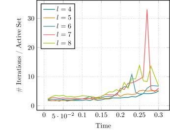
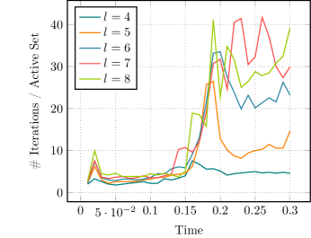
Figure 3: Multiple fractures. Iterations of the linear solver per active set step over time for different refinement levels $l$ with $\varepsilon=h$. Left: no stress splitting, right: Miehe-type stress splitting.

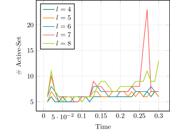
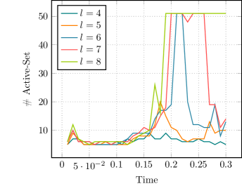
Figure 4: Multiple fractures (Example 1). Number of Active-Set steps over time for different refinement levels $l$ with $\varepsilon=h$. Left: no splitting. Right: Miehe-splitting.

Figure 5 shows the resulting fracture using randomly perturbed values for the elastic modulus. The random variations range from $0.1$ to $1$-times the original value, indicated by the image on the right. There, black denotes large values of elastic modulus, whereas white denotes small values. It can be observed that the resulting fracture avoids the high elastic modulus regions.

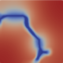
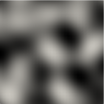
Figure 5: Multiple fractures. Fracture pattern using random variations in the elastic modulus ranging from $0.1$ (white) to $1$ (black) times the original value as shown in the right figure.

Matrix-free implementations are particularly suitable for parallelization. A first result into this direction is shown in Figure 6. There, the speed-up for a full simulation of the multiple fracture test with $0.8m$ and $3.2m$ dofs is shown. The parallel (strong) scaling using distributed parallelization is close to perfect down to a local problem size of roughly $25k$ dofs. When using more cores, the performance drops due to the increased overhead required for communication for smaller local problems. This allows us to reduce the computational time for the whole simulation from $400$ minutes down to $10$ minutes on $64$ cores for $l=7$. In the case of $l=8$, the simulation time drops from $35$ hours down to $23$ minutes using $128$ cores.

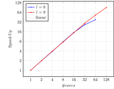
Figure 6: Multiple fractures. Speedup using distributed parallelization depending on the number of cores for a full simulation with $\varepsilon=h$ and roughly $0.8m$ and $3.2m$ dofs. Remarkably, the total number of iterations (Active-Set, linear) matches perfectly for all numbers of cores.

5.2 L-Shaped Panel

5.2.1 Problem Description

In this section, we consider the L-shaped panel test, which illustrates crack initiation and propagation without any predefined fractures.

The computational domain $\Omega_{L}$ is given by an L-shape $(0,500)^{2}\setminus\left((250,500)\times(0,250)\right)$, as depicted in Figure 7 (measures given in $mm$). Fracture propagation is driven by cyclic displacement boundary conditions $u_{y}(t)$ on $(500-30,500)\times\{250\}$, i.e. the lower boundary of the upper right part of the L-shape. The specimen is fixed on the lower part, i.e. $u=0\text{ on }(0,250)\times\{0\}$. No additional pressure is enforced inside the crack, hence $p=0$. The time-dependent displacement (given in $mm$) is defined by

$$u_{y}(t):=\begin{cases}t&0s\leq t<0.3s,\\ 0.6-t&0.3s\leq t<0.8s,\\ -1+t&0.8s\leq t<2s,\end{cases}$$

leading to a final displacement of $1mm$ after $2s$. A constant time-step of $dt:=10^{-3}$ was employed. Again, we chose $\varepsilon:=h$ for the fracture parameter. The load is evaluated on the top boundary $\Gamma_{up}:=(0,500)\times\{500\}$. The full list of parameters is summarized in Tables 3 and 4. Figure 8 shows the resulting crack pattern at different points in time.

Figure 7: L-shaped panel test. Geometry and cyclic displacement boundary conditions for the L-shaped panel test.

$l$	dofs	elements	$h$	$\varepsilon$
$5$	$2.5\cdot 10^{3}$	$7.7\cdot 10^{2}$	$2.2\cdot 10^{1}$	$2.2\cdot 10^{1}$
$6$	$9.6\cdot 10^{3}$	$3.1\cdot 10^{3}$	$1.1\cdot 10^{1}$	$1.1\cdot 10^{1}$
$7$	$3.8\cdot 10^{4}$	$1.2\cdot 10^{4}$	$5.5\cdot 10^{0}$	$5.5\cdot 10^{0}$
$8$	$1.5\cdot 10^{5}$	$4.9\cdot 10^{4}$	$2.8\cdot 10^{0}$	$2.8\cdot 10^{0}$

Table 3: L-Shaped Panel. Important values and parameters for different refinement levels $l$.

Variable	Value	Unit
$\mu$	$10.95$	$[kN/mm^{2}]$
$\lambda$	$6.16$	$[kN/mm^{2}]$
$G_{c}$	$8.9\cdot 10^{-5}$	$[kN/mm]$
$\kappa$	$10^{-10}$	$[1]$
$\varepsilon$	$11$	$[mm]$
$dt\ [s]$	$10^{-3}$	$[s]$

Table 4: L-Shaped Panel. Parameters.

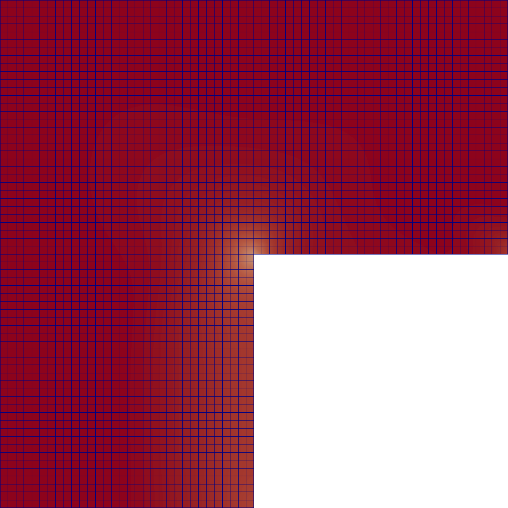
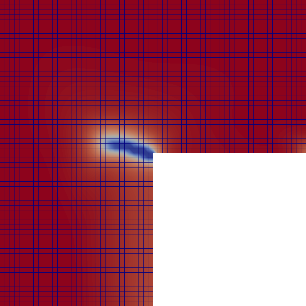
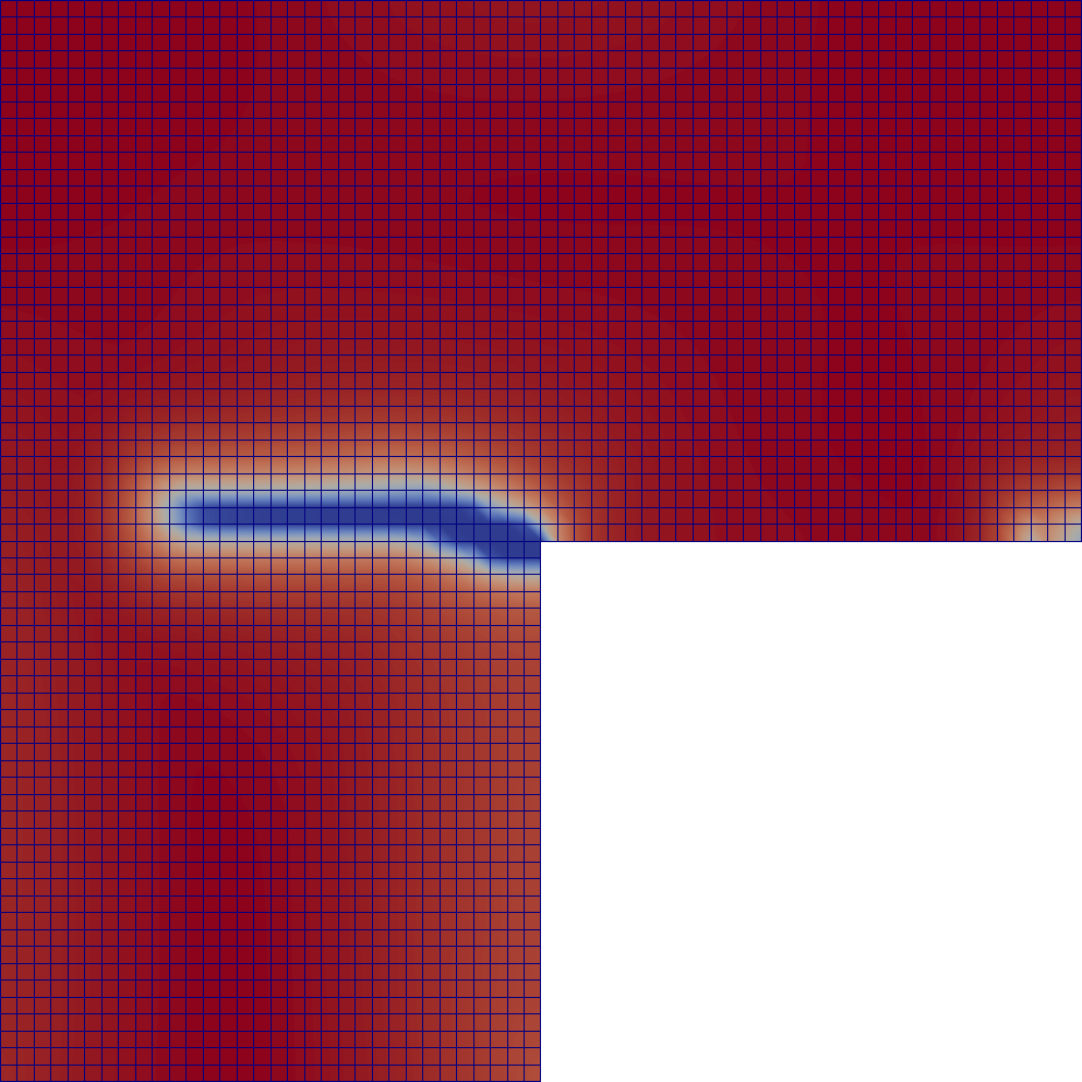
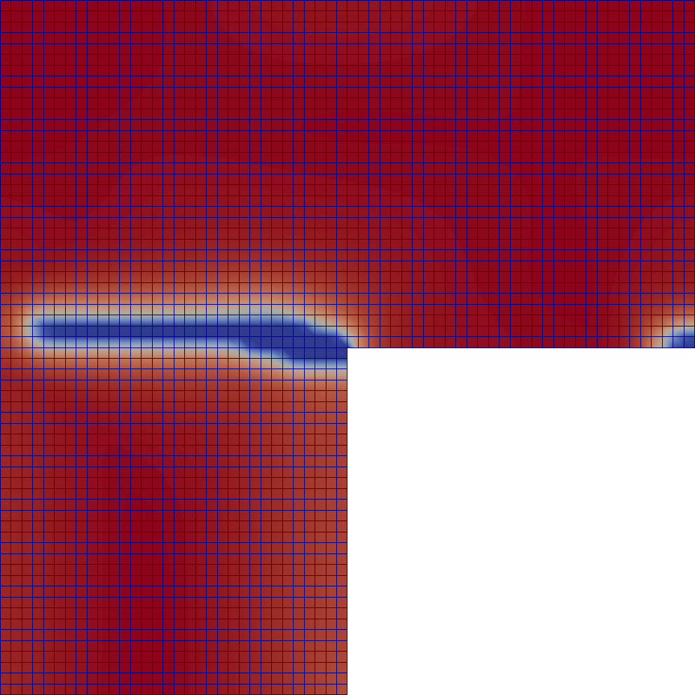
Figure 8: L-Shaped Panel. Resulting fracture pattern at times $t=0.22s,t=0.3s$ (top) and $t=1.45s,t=2s$ (bottom)

5.2.2 Numerical Results

For this second test, the number of Active-Set iterations is shown for $\varepsilon=h$ and $\varepsilon=22.0$. Random peaks happen in either case, but seem to cluster at different times. The iterations counts increase with higher levels towards the end of the simulation in case of constant $\varepsilon$. The $h$-dependent scenario is more robust in this regard.

The number of GMRES iterations presented in Figure 10 shows similar characteristics as before. Again, the iteration counts increase once the fracture starts growing at $t\sim 0.3s$ and again at $t\sim 0.8s$. In the first half of the simulation, our linear solver is robust with respect to $h$-refinement. During the second half, the number of iterations increases mildly on refinement in the case of $\varepsilon=h$, but stays almost constant for $\varepsilon=const$. On the finest grid ($l=8$), a huge increase can be observed in either case at $t\sim 0.8s$. in case of constant $\varepsilon$, such irregular behavior can also be observed in the first half of the simulation.

These results were obtained using the Miehe splitting, but similar findings were gathered for the Amor splitting. The solver also works if no splitting is applied ($\sim 2-7$ iterations), however, no crack initiation occurred in this case.

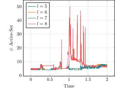
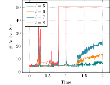
Figure 9: L-shaped panel. Number of Active-Set steps over time for different refinement levels $l$ with $\varepsilon=h$ and $\varepsilon=22mm$ (right).

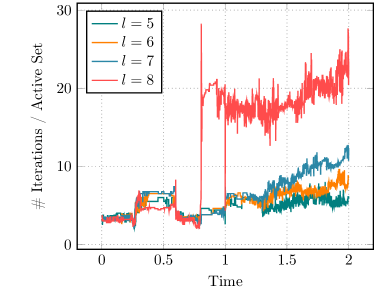
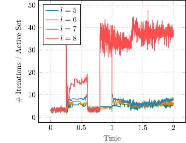
Figure 10: L-shaped panel. Iterations of the linear solver per active set step over time for different refinement levels $l$ with $\varepsilon=h$ (left) and $\varepsilon=22mm$ (right).

Figure 11 shows the load-displacement curves for different refinement levels. Our findings look similar to results found in literature in case of $\varepsilon=h$. Since the phase-field parameter $\varepsilon$ changes during refinement, convergence of the loading curves is not necessarily expected. Nonetheless, the overall shape of the presented curves agree mostly on each other. A major difference happens on the finest grid ($l=8$), where the load drops to zero at the turning point $u=-0.2m$, which does not happen on the coarser levels.

The same effect is also observed in the right image of Figure 11 (constant $\varepsilon$). In addition, the refinements $l=7$ and $l=8$ yield negative loading values during the second cycle, which is not as expected. Furthermore, small irregularities are visible at turning points, i.e. step-like curves somewhere between displacements of $0.2-0.4mm$. Similar artifacts are also visible in the crack and bulk-energy, see Figures 12 and 13. This test case seems to be very sensitive to the actual choice of parameters, elements and meshes, which is also reported in [71, 53].

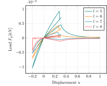
Figure 11: L-shaped panel. Load – displacement curves for different refinement levels $l$. The left image shows the results for $\varepsilon=h$, whereas on the right we have a fixed value $\varepsilon=22$.

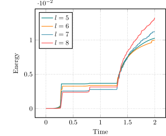
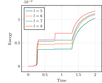
Figure 12: L-shaped panel. Crack energy for different refinement levels $l$ with $\varepsilon=h$ (left) and $\varepsilon=22$ (right).

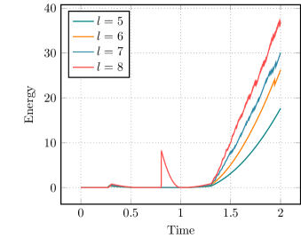
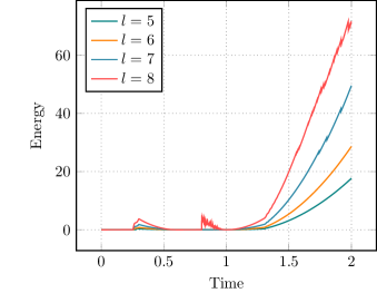
Figure 13: L-shaped panel. Bulk energy for different refinement levels $l$ with $\varepsilon=h$ (left) and $\varepsilon=22$ (right).

5.3 $3d$ L-Shaped Panel

5.3.1 Problem Description

In this section, we consider a $3d$ version of the previous L-shaped panel test. A related numerical study is [55]. A related experimental test was previously proposed in [75]. The computational domain is given by extruding $\Omega_{L}$ from before into z-direction. Hence, $\Omega_{L}^{3d}:=\Omega_{L}\times(0,250)$, as depicted in Figure 14 (measures given in $mm$). The same cyclic displacement boundary conditions are applied as before on the extruded area $(500-30,500)\times\{250\}\times(0,250)$. The specimen is fixed on the bottom, i.e. $u=0\text{ on }(0,250)\times\{0\}\times(0,250)$. Again, the loading force is evaluated on the upper boundary $\Gamma_{up}:=(0,500)\times\{500\}\times(0,250)$. The full list of parameters is summarized in Tables 5 and 6. Figure 15 illustrates the resulting fracture.

Figure 14: $3d$ L-shaped panel. Geometry and loading for the L-shaped panel test.

$l$	dofs	elements	$h$	$\varepsilon$
$4$	$8.1\cdot 10^{3}$	$1.5\cdot 10^{3}$	$5.4\cdot 10^{1}$	$5.4\cdot 10^{1}$
$5$	$5.7\cdot 10^{4}$	$1.2\cdot 10^{4}$	$2.7\cdot 10^{1}$	$2.7\cdot 10^{1}$
$6$	$4.2\cdot 10^{5}$	$9.8\cdot 10^{4}$	$1.4\cdot 10^{1}$	$1.4\cdot 10^{1}$
$7$	$3.3\cdot 10^{6}$	$7.9\cdot 10^{5}$	$6.8\cdot 10^{0}$	$6.8\cdot 10^{0}$

Table 5: $3d$ L-Shaped Panel. Important values and parameters for different refinement levels $l$.

Variable	Value	Unit
$\mu$	$10.95$	$[kN/mm^{2}]$
$\lambda$	$6.16$	$[kN/mm^{2}]$
$G_{c}$	$8.9\cdot 10^{-5}$	$[kN/mm]$
$\kappa$	$10^{-10}$	$[1]$
$\varepsilon$	$11$	$[mm]$
$dt\ [s]$	$10^{-3}$	$[s]$

Table 6: $3d$ L-Shaped Panel. Parameters.

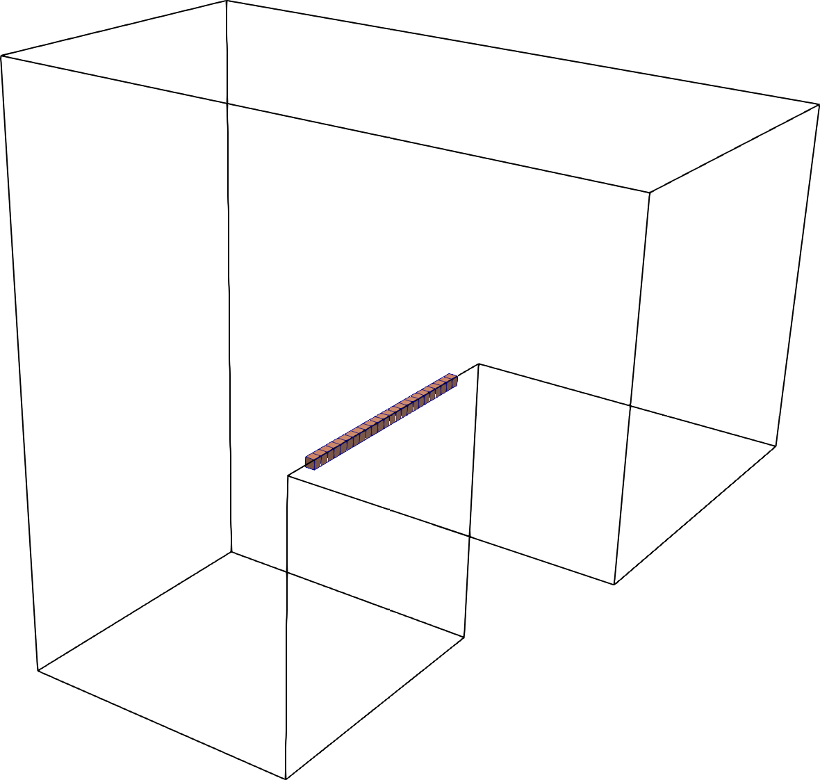
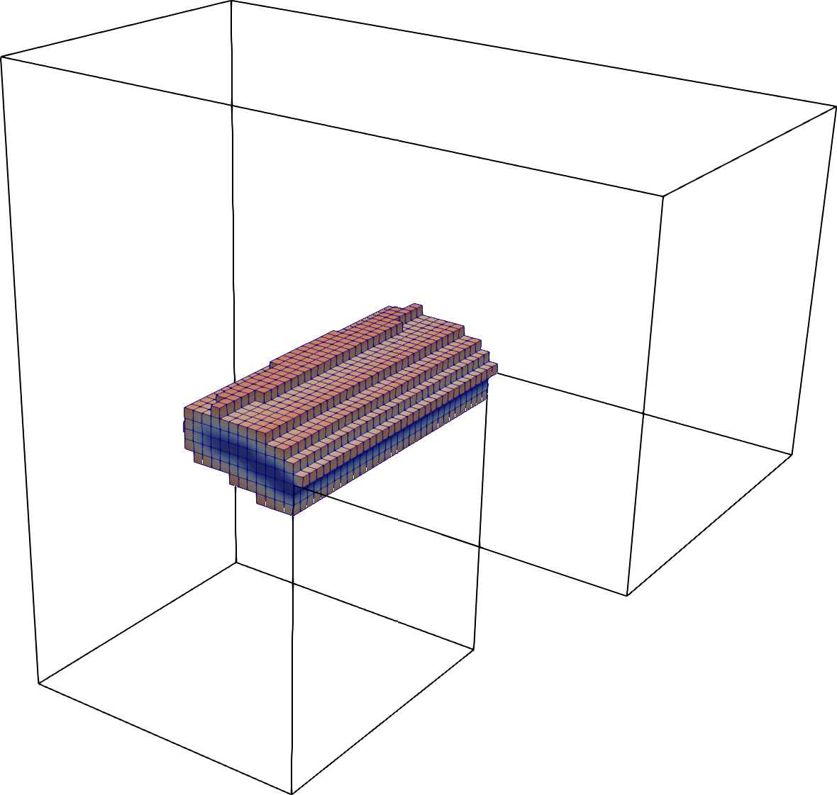
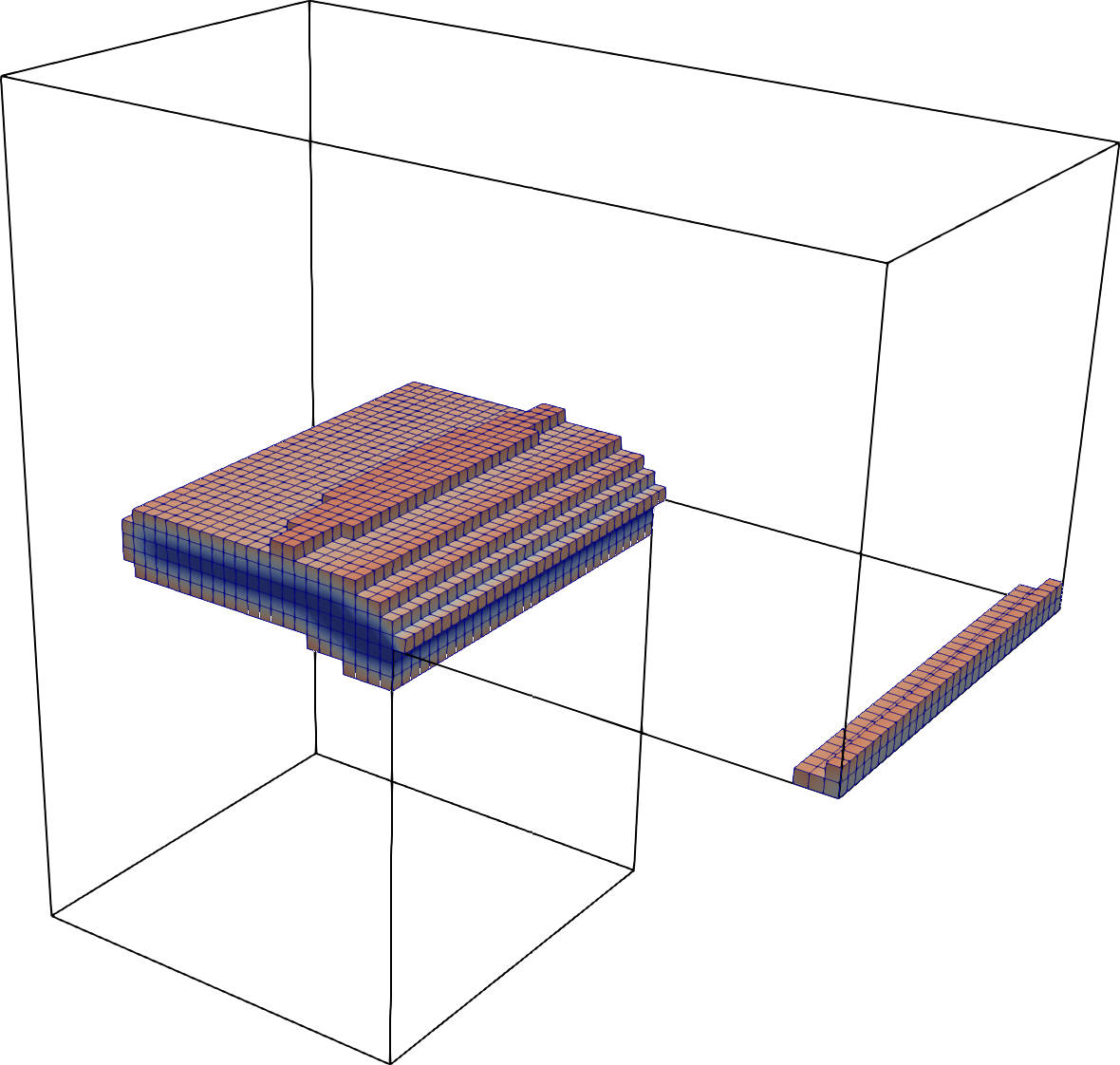
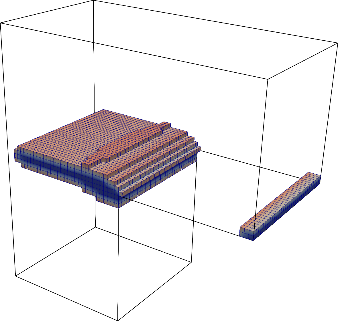
Figure 15: $3d$ L-Shaped Panel. Resulting fracture pattern at times $t=0.22s,t=0.3s$ (top) and $t=1.45s,t=2s$ (bottom). Only parts with $\varphi<0.75$ are shown.

5.3.2 Numerical Results

The results for the $3d$ extension of the L-shaped panel test are very similar to the previously shown $2d$ setup. The number of Active-Set iterations is in the same range as before, but less peaks are visible in the $3d$ setting, see Figure 16 (left). Figure 16 (right) shows that the number of GMRES iterations per Active-Set step is in again very similar, i.e. roughly $4-10$ iterations.

We also observe a similarly increased iteration count at times when the fracture is growing.

Also, the shape of energy and loading curves (Figures 17 and 18) look very similar in the $2d$ and $3d$ case. The exception being the coarsest $3d$ grid, which shows a very roundly shaped loading curve, which does not agree with the $2d$ setting. However, the numbers do not even remotely agree, as seen in Figures 17 and 18.

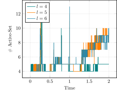
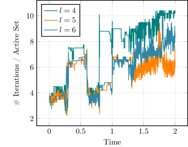
Figure 16: $3d$ L-shaped panel. Left: number of Active-Set iterations over time. Right: number of iterations of the linear solver per active set step over time for different refinement levels $l$ with $\varepsilon=h$.

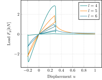
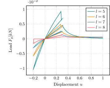
Figure 17: $3d$ L-shaped panel. Load – displacement curves for different refinement levels $l$ in the $3d$ case (left). For comparison, we show the respective results for $2d$ case again (right).

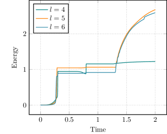
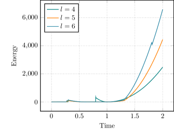
Figure 18: $3d$ L-shaped panel. Crack and bulk energy for different refinement levels $l$ with $\varepsilon=h$.

6 Conclusions and Future Work

In this work, we developed a matrix-free geometric multigrid solver for fracture propagation problems using a phase-field description. Our numerical experiments show that this solver can handle a variety of test cases within a reasonable number of iterations. Although we have only shown results for the AT 2 model, it shall be noted that the solver also works for the simpler AT 1 model, with iteration counts usually below the presented values. Limitations of this method appear primary in case of stress-splittings. The improvement of the solver in these cases is part of our future work. In order to deal with larger simulations (in particular in 3d), incorporating adaptivity and/or parallelization is necessary; both of which are part of our ongoing work. Another point of concern is the Active-Set method. In some simulations, convergence of this non-linear solver is observed to be very slow as also indicated in fundamental studies on primal-dual active set methods, e.g., [34, 22]. Hence, it may be beneficial to further investigate properties of the active set method with the goal of further improvements. Ultimately, one could also think of combining the non-linear and linear solver in terms of nested iterations or non-linear multigrid methods (see e.g. [47, 31]).

7 Acknowledgments

This work has been supported by the Austrian Science Fund (FWF) grant P29181 ‘Goal-Oriented Error Control for Phase-Field Fracture Coupled to Multiphysics Problems’.

References

- [1] Mark Adams, Marian Brezina, Jonathan Hu and Ray Tuminaro “Parallel multigrid smoothing: Polynomial versus Gauss-Seidel” In Journal of Computational Physics 80309.1, 2003, pp. 1–19
- [2] G. Alzetta et al. “The deal.II Library, Version 9.0” In Journal of Numerical Mathematics 26.4, 2018, pp. 173–183
- [3] Marreddy Ambati, Tymofiy Gerasimov and Laura De Lorenzis “A review on phase-field models of brittle fracture and a new fast hybrid formulation” In Computational Mechanics 55.2 Springer Berlin Heidelberg, 2015, pp. 383–405
- [4] L Ambrosio and V M Tortorelli “Approximation of functionals depending on jumps by elliptic functionals via Gamma-convergence” In Comm. Pure Appl. Math. 43, 1990, pp. 999–1036
- [5] L Ambrosio and V M Tortorelli “On the approximation of free discontinuity problems” In Boll. Un. Mat. Ital. B 6, 1992, pp. 105–123
- [6] H Amor, J.-J. Marigo and C Maurini “Regularized formulation of the variational brittle fracture with unilateral contact: Numerical experiments” In J. Mech. Phys. Solids 57, 2009, pp. 1209–1229
- [7] Auburns “FastNoise” In GitHub repository GitHub, https://github.com/Auburns/FastNoise, 2018
- [8] Allison H. Baker, Robert D. Falgout, Tzanio V. Kolev and Ulrike Meier Yang “Multigrid Smoothers for Ultraparallel Computing” In SIAM J. Sci. Comput. 33.5 Society for IndustrialApplied Mathematics, 2011, pp. 2864–2887
- [9] Wolfgang Bangerth, Ralf Hartmann and Guido Kanschat “deal.II – a General Purpose Object Oriented Finite Element Library” In ACM Trans. Math. Softw. 33.4, 2007, pp. 24/1–24/27
- [10] V. Belsky “A multi-grid method for variational inequalities in contact problems” In Computing 51.3, 1993, pp. 293–311
- [11] Ted Belytschko and T. Black “Elastic Crack Growth With Minimal Remeshing” In International Journal for Numerical Methods in Engineering 45.5, 1999, pp. 610–620
- [12] P.. Bernard, N. Moës and N. Chevaugeon “Damage growth modeling using the Thick Level Set (TLS) approach: Efficient discretization for quasi-static loadings” In Computer Methods in Applied Mechanics and Engineering 233-236 Elsevier B.V., 2012, pp. 11–27
- [13] H Blum, Dietrich Braess and F T Suttmeier “A cascadic multigrid algorithm for variational inequalities” In Computing and Visualization in Science 7.3, 2004, pp. 153–157
- [14] M J Borden et al. “A phase-field description of dynamic brittle fracture” In Comput. Meth. Appl. Mech. Engrg. 217, 2012, pp. 77–95
- [15] B Bourdin “Numerical implementation of the variational formulation for quasi-static brittle fracture” In Interfaces and free boundaries 9, 2007, pp. 411–430
- [16] B Bourdin, G A Francfort and J.-J. Marigo “Numerical experiments in revisited brittle fracture” In J. Mech. Phys. Solids 48.4, 2000, pp. 797–826
- [17] Blaise Bourdin, Jean-Jacques Marigo, Corrado Maurini and Paul Sicsic “Morphogenesis and Propagation of Complex Cracks Induced by Thermal Shocks” In Phys. Rev. Lett. 112 American Physical Society, 2014, pp. 014301
- [18] James H. Bramble “Multigrid methods” CRC Press, 1993
- [19] S. Brunssen, F. Schmid, M. Schäfer and Barbara Wohlmuth “A fast and robust iterative solver for nonlinear contact problems using a primal-dual active set strategy and algebraic multigrid” In International Journal for Numerical Methods in Engineering 69.3, 2007, pp. 524–543
- [20] S. Burke, Ch. Ortner and E. Süli “An adaptive finite element approximation of a variational model of brittle fracture” In SIAM J. Numer. Anal. 48.3, 2010, pp. 980–1012
- [21] Chukwudi Chukwudozie, Blaise Bourdin and Keita Yoshioka “A variational phase-field model for hydraulic fracturing in porous media” In Computer Methods in Applied Mechanics and Engineering 347, 2019, pp. 957–982
- [22] Frank E. Curtis, Zheng Han and Daniel P. Robinson “A globally convergent primal-dual active-set framework for large-scale convex quadratic optimization” In Computational Optimization and Applications 60.2, 2015, pp. 311–341
- [23] Patrick E Farrell and Corrado Maurini “Linear and nonlinear solvers for variational phase-field models of brittle fracture” In International Journal for Numerical Methods in Engineering 109.5, 2017, pp. 648–667 arXiv:1010.1724
- [24] C. Feist and G. Hofstetter “An embedded strong discontinuity model for cracking of plain concrete” In Computer Methods in Applied Mechanics and Engineering 195.52, 2006, pp. 7115–7138
- [25] G A Francfort and J.-J. Marigo “Revisiting brittle fracture as an energy minimization problem” In J. Mech. Phys. Solids 46.8, 1998, pp. 1319–1342
- [26] M.. Gee et al. “ML 5.0 Smoothed Aggregation User’s Guide”, 2006
- [27] Tymofiy Gerasimov and Laura De Lorenzis “A line search assisted monolithic approach for phase-field computing of brittle fracture” In Computer Methods in Applied Mechanics and Engineering 312 Elsevier B.V., 2016, pp. 276–303
- [28] C. Gräser and O. Sander “Truncated Nonsmooth Newton Multigrid Methods for Block-Separable Minimization Problems” In IMA Journal of Numerical Analysis, 2019
- [29] Alan Arnold Griffith and Geoffrey Ingram Taylor “The phenomena of rupture and flow in solids” In Philosophical Transactions of the Royal Society of London. Series A, Containing Papers of a Mathematical or Physical Character 221.582-593, 1921, pp. 163–198
- [30] G. Haase and U. Langer “Modern Methods in Scientific Computing and Applications” 75, NATO Science Series II. Mathematics, Physics and Chemistry Kluwer Academic Press, 2002, pp. 103–154
- [31] Wolfgang Hackbusch “Multi-Grid Methods” In Iterative Solution of Large Sparse Systems of Equations Springer New York, 1994, pp. 296–366
- [32] Wolfgang Hackbusch “Multi-Grid Methods and Applications” Springer-Verlag, 1985
- [33] Wolfgang Hackbusch and Hans D. Mittelmann “On multi-grid methods for variational inequalities” In Numerische Mathematik 42.1, 1983, pp. 65–76
- [34] Zheng Han “Primal-dual active-set methods for convex quadratic optimization with applications”, 2015
- [35] Y. Heider and B. Markert “A phase-field modeling approach of hydraulic fracture in saturated porous media” In Mechanics Research Communications 80 Elsevier Ltd., 2017, pp. 38–46
- [36] Timo Heister, M F Wheeler and Thomas Wick “A primal-dual active set method and predictor-corrector mesh adaptivity for computing fracture propagation using a phase-field approach” In Computer Methods in Applied Mechanics and Engineering 290.0 Elsevier B.V., 2015, pp. 466–495
- [37] Timo Heister and Thomas Wick “Parallel solution, adaptivity, computational convergence, and open-source code of 2d and 3d pressurized phase-field fracture problems” In PAMM 18.1, 2018, pp. e201800353 eprint: https://onlinelibrary.wiley.com/doi/pdf/10.1002/pamm.201800353
- [38] Ingo Heppner et al. “Software Framework ug4: Parallel Multigrid on the Hermit Supercomputer” In High Performance Computing in Science and Engineering ‘12 Springer Berlin Heidelberg, 2013, pp. 435–449
- [39] M. Heroux et al. “An Overview of Trilinos”, 2003
- [40] Michael Hintermüller, Kazufumi Ito and Karl Kunisch “The primal-dual active set strategy as a semismooth Newton method” In SIAM J. Optim. 13.3, 2003, pp. 865–888
- [41] Ronald H.. Hoppe “Multigrid Algorithms for Variational Inequalities” In SIAM Journal on Numerical Analysis 24.5, 1987, pp. 1046–1065
- [42] Ronald H.. Hoppe and Hans D. Mittelmann “A multi-grid continuation strategy for parameter-dependent variational inequalities” In Journal of Computational and Applied Mathematics 26.1, 1989, pp. 35–46
- [43] Kazufumi Ito and Karl Kunisch “Augmented Lagrangian methods for nonsmooth , convex optimization in Hilbert spaces”, 2000, pp. 591–616
- [44] Ralf Kornhuber “Monotone multigrid methods for elliptic variational inequalities I” In Numerische Mathematik 69.2, 1994, pp. 167–184
- [45] Ralf Kornhuber “On constrained Newton linearization and multigrid for variational inequalities” In Numerische Mathematik 91.4, 2002, pp. 699–721
- [46] Ralf Kornhuber and C. Gräser “Multigrid methods for obstacle problems” In J. Comp. Math. 27.1, 2009, pp. 1–44
- [47] R. Krause “From inexact active set strategies to nonlinear multigrid methods” In Analysis and Simulation of Contact Problems Springer Berlin Heidelberg, 2006, pp. 13–21
- [48] Martin Kronbichler and Katharina Kormann “A generic interface for parallel cell-based finite element operator application” In Computers & Fluids 63, 2012, pp. 135–147
- [49] Martin Kronbichler and Katharina Kormann “Fast matrix-free evaluation of discontinuous Galerkin finite element operators”, 2017 arXiv:1711.03590
- [50] Charlotte Kuhn, Alexander Schlüter and Ralf Müller “On degradation functions in phase field fracture models” In Computational Materials Science 108, 2015, pp. 374–384
- [51] S Lee, M F Wheeler and T Wick “Iterative coupling of flow, geomechanics and adaptive phase-field fracture including level-set crack width approaches” In Journal of Computational and Applied Mathematics 314, 2017, pp. 40–60
- [52] S Lee, Mary F Wheeler and T Wick “Pressure and fluid-driven fracture propagation in porous media using an adaptive finite element phase field model” In Computer Methods in Applied Mechanics and Engineering 305, 2016, pp. 111–132
- [53] K. Mang, T. Wick and W. Wollner “A phase-field model for fractures in incompressible solids”, 2019
- [54] Günther Meschke and Peter Dumstorff “Energy-based modeling of cohesive and cohesionless cracks via X-FEM” In Computer Methods in Applied Mechanics and Engineering 196.21-24, 2007, pp. 2338–2357
- [55] A. Mesgarnejad, B. Bourdin and M.. Khonsari “Validation simulations for the variational approach to fracture” In Computer Methods in Applied Mechanics and Engineering 290 Elsevier B.V., 2015, pp. 420–437
- [56] C Miehe, M Hofacker and F Welschinger “A phase field model for rate-independent crack propagation: Robust algorithmic implementation based on operator splits” In Comput. Meth. Appl. Mech. Engrg. 199, 2010, pp. 2765–2778
- [57] C Miehe, F Welschinger and M Hofacker “Thermodynamically consistent phase-field models of fracture: variational principles and multi-field FE implementations” In Int. J. Numer. Methods Engrg. 83, 2010, pp. 1273–1311
- [58] Christian Miehe and Steffen Mauthe “Phase field modeling of fracture in multi-physics problems. Part III. Crack driving forces in hydro-poro-elasticity and hydraulic fracturing of fluid-saturated porous media” In Computer Methods in Applied Mechanics and Engineering 304 Elsevier B.V., 2016, pp. 619–655
- [59] Christian Miehe, Steffen Mauthe and Stephan Teichtmeister “Minimization principles for the coupled problem of Darcy–Biot-type fluid transport in porous media linked to phase field modeling of fracture” In Journal of the Mechanics and Physics of Solids 82, 2015, pp. 186–217
- [60] A Mikelić, M.. Wheeler and T Wick “A phase-field method for propagating fluid-filled fractures coupled to a surrounding porous medium” In SIAM Multiscale Model. Simul. 13.1, 2015, pp. 367–398
- [61] A Mikelić, M.. Wheeler and T Wick “A quasi-static phase-field approach to pressurized fractures” In Nonlinearity 28.5, 2015, pp. 1371–1399
- [62] A. Mikelić, M.. Wheeler and T. Wick “Phase-field modeling through iterative splitting of hydraulic fractures in a poroelastic medium” In GEM - International Journal on Geomathematics 10.1, 2019
- [63] Sebastian Reiter et al. “A massively parallel geometric multigrid solver on hierarchically distributed grids” In Computing and Visualization in Science 16.4, 2013, pp. 151–164
- [64] Yousef Saad “Iterative Methods for Sparse Linear Systems Second Edition Yousef Saad” In Philadelphia, Pennsylvania: SIAM, 2003, pp. 421–426 arXiv:0806.3802
- [65] Yousef Saad and M.. Schultz “GMRES: A generalized minimal residual algorithm for solving nonsymmetric linear systems” In SIAM Journal on Scientific and Statistical Computing 7.3, 1986, pp. 856–869
- [66] N. Singh, C.V. Verhoosel and E.H. van Brummelen “Finite element simulation of pressure-loaded phase-field fractures” In Meccanica 53.6 Springer, 2018, pp. 1513–1545
- [67] K. Stüben “A review of algebraic multigrid” In Journal of Computational and Applied Mathematics 128.1, 2001, pp. 281–309
- [68] Jörg F Unger, Stefan Eckardt and Carsten Könke “Modelling of cohesive crack growth in concrete structures with the extended finite element method” In Computer Methods in Applied Mechanics and Engineering 196.41, 2007, pp. 4087–4100
- [69] Richard S Varga “Matrix Iterative Analysis” In USSR Computational Mathematics and Mathematical Physics 5, 1999
- [70] T. Wick, G. Singh and M.F. Wheeler “Fluid-filled fracture propagation using a phase-field approach and Coupling to a reservoir simulator” In SPE Journal 21.03, 2016, pp. 981–999
- [71] Thomas Wick “An Error-Oriented Newton/Inexact Augmented Lagrangian Approach for Fully Monolithic Phase-Field Fracture Propagation” In SIAM Journal on Scientific Computing 39.4, 2017, pp. B589–B617
- [72] Thomas Wick “Modified Newton methods for solving fully monolithic phase-field quasi-static brittle fracture propagation” In Computer Methods in Applied Mechanics and Engineering 325.July, 2017, pp. 577–611
- [73] Zachary A. Wilson and Chad M. Landis “Phase-field modeling of hydraulic fracture” In Journal of the Mechanics and Physics of Solids 96, 2016, pp. 264–290
- [74] Zachary Adam Wilson “Phase-field Modeling of Fracture for Multiphysics Problems”, 2016
- [75] B.. Winkler “Traglastuntersuchungen von unbewehrten und bewehrten Betonstrukturen auf der Grundlage eines objectiven Werkstoffgesetzes für Beton”, 2001
- [76] Keita Yoshioka and Blaise Bourdin “A variational hydraulic fracturing model coupled to a reservoir simulator” In International Journal of Rock Mechanics and Mining Sciences 88, 2016, pp. 137–150