Addressing the $\mathbf{\textit{R}}_{\mathbf{\textit{D}}^{(*)}}$ anomalies with an $\mathbf{\textit{S}_{1}}$ leptoquark from $\mathbf{SO(10)}$ grand unification

Abstract

Motivated by the $R_{D^{(*)}}$ anomalies, we investigate an $\mathrm{SO}(10)$ grand unification scenario where a charge $-1/3$ scalar leptoquark ($S_{1}$) remains as the only new physics candidate at the TeV scale. This leptoquark along with the Standard Model (SM) Higgs doublet originates from the same ten-dimensional real scalar multiplet in the $\mathrm{SO}(10)$ grand unification framework taking its mass close to the electroweak scale. We explicitly show how the gauge coupling unification is achieved with only one intermediate symmetry-breaking scale at which the Pati-Salam gauge group is broken into the SM group. We investigate the phenomenological implications of our scenario and show that an $S_{1}$ with a specific Yukawa texture can explain the $R_{D^{(*)}}$ anomalies. We perform a multiparameter scan considering the relevant flavour constraints on $R_{D^{(*)}}$, $F_{L}{(D^{*})}$, $P_{\tau}(D^{*})$ and $R_{K^{(*)}}^{\nu\nu}$ as well as the constraint coming from the $Z\to\tau\tau$ decay and the latest $\tau\tau$ resonance search data at the LHC. Our analysis shows that a single leptoquark solution to the observed $R_{D^{(*)}}$ anomalies with $S_{1}$ is still a viable solution.

I Introduction

During the past few years, several disagreements between experiments and the Standard Model (SM) predictions in the rare $B$ decays have been reported by the BaBar Lees:2012xj ; Lees:2013uzd , LHCb Aaij:2014ora ; Aaij:2017vbb ; Aaij:2015yra ; Aaij:2017uff ; Aaij:2017deq and Belle Huschle:2015rga ; Sato:2016svk ; Hirose:2016wfn ; Hirose:2017dxl collaborations. So far, these anomalies have been quite persistent. The most significant ones have been observed in the $R_{D^{(*)}}$ and $R_{K^{(*)}}$ observables, defined as,

$$R_{D^{(*)}} = \dfrac{\mathrm{BR}(B\rightarrow D^{(*)}\tau\nu)}{\mathrm{BR}(B\rightarrow D^{(*)}\ell\nu)}\quad\mbox{and}$$

$$R_{K^{(*)}} = \dfrac{\mathrm{BR}(B\rightarrow K^{(*)}\mu^{+}\mu^{-})}{\mathrm{BR}(B\rightarrow K^{(*)}e^{+}e^{-})}\;.$$

Here, $\ell=\{e$ or $\mu\}$ and $\mathrm{BR}$ stands for branching ratio. The experimental values of $R_{D}$ and $R_{D^{*}}$ are in excess of their SM predictions Bigi:2016mdz ; Bernlochner:2017jka ; Bigi:2017jbd ; Jaiswal:2017rve by $1.4\sigma$ and $2.5\sigma$, respectively, (combined excess of $3.08\sigma$ in $R_{D^{(*)}}$) based on the world averages as of spring 2019, according to the Heavy Flavor Averaging Group Amhis:2016xyh , whereas, the observed $R_{K}$ and $R_{K^{*}}$ are both suppressed compared to their SM predictions Hiller:2003js ; Bordone:2016gaq by $\sim 2.6\sigma$.

One of the possible explanations for the $B$-decay anomalies is the existence of scalar leptoquarks whose masses are in the few-TeV range Dorsner:2013tla ; Sakaki:2013bfa ; Freytsis:2015qca ; Bauer:2015knc ; Dumont:2016xpj ; Das:2016vkr ; Becirevic:2016oho ; Becirevic:2016yqi ; Faroughy:2016osc ; Hiller:2016kry ; Chen:2017hir ; Crivellin:2017zlb ; Becirevic:2017jtw ; Cai:2017wry ; Altmannshofer:2017poe ; Assad:2017iib ; Jung:2018lfu ; Biswas:2018jun ; Bandyopadhyay:2018syt ; Aydemir:2018cbb ; Marzocca:2018wcf ; Becirevic:2018afm ; Kumar:2018kmr ; Hu:2018lmk ; Faber:2018qon ; Heeck:2018ntp ; Angelescu:2018tyl ; Bifani:2018zmi ; Bansal:2018nwp ; Mandal:2018kau ; Iguro:2018vqb ; Aebischer:2018acj ; Bar-Shalom:2018ure ; Kim:2018oih ; Arnan:2019olv ). Leptoquarks, which posses both lepton and quark couplings, often exist in the grand unified theories (GUTs) or in the Pati-Salam-type models. Considering that the LHC searches, except for these anomalies, have so far returned empty handed, if the leptoquarks indeed turn out to be behind these anomalies, it is likely that there will only be a small number of particles to be discovered. However, their existence in small numbers at the TeV scale would be curious in terms of its implications regarding physics beyond the Standard Model. Scalars in these models mostly come in large multiplets and it would be peculiar that only one or a few of the components become light at the TeV scale while others remain heavy. Mass splitting is actually a well-speculated subject in the literature in the context of the infamous doublet-triplet splitting problem in supersymmetric theories and GUTs. From this point of view, even the SM Higgs in a GUT framework is troublesome if it turns out to be the only scalar at the electroweak (EW) scale.

In this paper, we consider a single scalar leptoquark, $S_{1}(3,1,-1/3)$, at the TeV scale, in the $\mathrm{SO}(10)$ GUT framework Fritzsch:1974nn ; Georgi:1974my ; Chang:1983fu ; Chang:1984uy ; Chang:1984qr ; Deshpande:1992au ; Bajc:2005zf ; Bertolini:2009qj ; Babu:2012vc ; Altarelli:2013aqa ; Aydemir:2015oob ; Aydemir:2016qqj ; Babu:2015bna ; Babu:2016bmy . This particular leptoquark was discussed in the literature to be responsible for one (or possibly both) of the $R_{D^{(*)}}$ and $R_{K^{(*)}}$ anomalies Bauer:2015knc ; Becirevic:2016oho ; Cai:2017wry ; Freytsis:2015qca . (Later, however, it was shown in Ref. Angelescu:2018tyl that a single $S_{1}$ leptoquark can only alleviate the $R_{K^{(*)}}$ discrepancy, but cannot fully resolve it.) Furthermore, it is contained in a relatively small multiplet that resides in the fundamental representation of the $\mathrm{SO}(10)$ group, a real $\mathbf{10}$, together with a scalar doublet with the quantum numbers that allow it to be identified as the SM Higgs. Therefore, $S_{1}$ being the only light scalar entity other than the SM Higgs doublet is justified in this scenario. A future discovery of such a leptoquark at the TeV scale could be interpreted as evidence in favour of an $\mathrm{SO}(10)$ GUT.

It has been argued in the literature that a real $\mathbf{10}_{H}$ in the minimal $\mathrm{SO}(10)$ setup (even together with a real $\mathbf{120}_{H}$ or a complex $\mathbf{120}_{H}$) is not favoured in terms of a realistic Yukawa sector Bajc:2005zf . On the other hand, it has been recently discussed in Ref. Babu:2016bmy that a Yukawa sector consisting of a real $\mathbf{10}_{H}$, a real $\mathbf{120}_{H}$ and a complex $\mathbf{126}_{H}$, can establish a realistic Yukawa sector due to the contributions from the scalars whose quantum numbers are the same as the SM Higgs doublet. Thus, this is the scalar content we assign in our model for the Yukawa sector.

The inclusion of $S_{1}$ in the particle content of the model at the TeV scale does not improve the status of the SM in terms of gauge coupling unification, which cannot be realized by the particle content in question. Fortunately, in the $\mathrm{SO}(10)$ framework, there are other ways to unify the gauge coupling constants, in contrast to models based on the $\mathrm{SU}(5)$ group which also contains such a leptoquark within the same multiplet as the SM Higgs. As we illustrate in this paper, inserting a single intermediate phase where the active gauge group is the Pati-Salam group, $\mathrm{SU}(4)_{\mathcal{C}}\otimes\mathrm{SU}(2)_{L}\otimes\mathrm{SU}(2)_{R}$, which appears to be the favoured route of symmetry-breaking by various phenomenological bounds Altarelli:2013aqa , establishes coupling unification as desired. In our model, the Pati-Salam group is broken into the SM gauge group at an intermediate energy scale $M_{C}$, while $\mathrm{SO}(10)$ is broken into the Pati-Salam group at the unification scale $M_{U}$. We consider two versions of this scenario, depending on whether the left-right symmetry, so-called $D$ parity, is broken together with $\mathrm{SO}(10)$ at $M_{U}$, or it is broken at a later stage, at $M_{C}$, where the Pati-Salam symmetry is broken into the SM gauge symmetry.

Light colour triplets, similar to the one we consider in this paper, are often dismissed for the sake of proton stability since these particles in general have the right quantum numbers for them to couple potentially dangerous operators that mediate proton decay. On the other hand, the proton stability could possibly be ensured through various symmetry mechanisms such as the utilization of Peccei-Quinn (PQ) symmetry Cox:2016epl ; Bajc:2005zf , other $\mathrm{U}(1)$ symmetries such as the one discussed in Ref. Pati:1974yy , or a discrete symmetry similar to the one considered in Ref. Bauer:2015knc . Operators leading to proton decay could also be suppressed by a specific mechanism such as the one discussed in Ref. Dvali:1995hp or they could be completely forbidden by geometrical reasons Aydemir:2018cbb . In this paper, we adopt a discrete symmetry as suggested in Ref.  Bauer:2015knc , assumed to operate below the intermediate symmetry-breaking scale even though it is not manifest at higher energies.

Motivated by the possible existence of a single TeV scale $S_{1}$ in the $\mathrm{SO}(10)$ GUT framework, we move on to investigate the phenomenological implications of our model. In Ref. Bauer:2015knc , it was shown that a TeV scale $S_{1}$ leptoquark can explain the $R_{D^{(*)}}$ anomalies while simultaneously inducing the desired suppression in $R_{K^{(*)}}$ through box diagrams. Since the most significant anomalies are seen in the $R_{D^{(*)}}$ observables, in this paper, we concentrate mostly on scenarios that can accommodate these observables. Generally, a TeV scale $S_{1}$ requires one Yukawa coupling to be large to accommodate the $R_{D^{(*)}}$ anomalies Cai:2017wry ; Angelescu:2018tyl . This, however, could create a problem for the $b\to s\bar{\nu}\nu$ transition rate measured in the $R_{K}^{\nu\nu}$ observable. In the SM, this decay proceeds through a loop whereas $S_{1}$ can contribute at the tree level in this transition. Therefore, the measurement of $R_{K}^{\nu\nu}$ is very important to restrict the parameter space of $S_{1}$. Some specific Yukawa couplings of $S_{1}$ are also severely constrained from the $Z\to\tau\tau$ decay Bansal:2018nwp and the LHC $\tau\tau$ resonance search data Mandal:2018kau . Therefore, it is evident that in order to find the $R_{D^{(*)}}$-favoured parameter space while successfully accommodating other relevant constraints, one has to introduce new degrees of freedom in terms of new couplings and/or new particles. Here, we consider a specific Yukawa texture with three free couplings to show that a TeV scale $S_{1}$, consistent with relevant measurements, can still explain the $R_{D^{(*)}}$ anomalies.

The rest of the paper is organized as follows. In Sec. II, we introduce our model. In Sec. III, we display the unification of the couplings for two versions of our model. In Sec. IV, we present the related LHC phenomenology with a single extra leptoquark $S_{1}$. We display the exclusion limits from the LHC data and discuss related future prospects. We also study the renormalization group (RG) running of the Yukawa couplings. Finally in Sec. V, we end our paper with a discussion and conclusions.

II The $\mathbf{SO(10)}$ model

In our $\mathrm{SO}(10)$ model, we entertain the idea that the SM Higgs doublet is not the only scalar multiplet at the TeV scale, but it is accompanied by a leptoquark $S_{1}=(3,1,-1/3)$, both of which reside in a real ten-dimensional representation, $\mathbf{10}$, of $\mathrm{SO}(10)$ group. The peculiar mass splitting among the components of this multiplet does not occur, leading to a naturally light scalar leptoquark at the TeV scale.

We start with a real $\mathbf{10}_{H}$ of $\mathrm{SO}(10)$ whose Pati-Salam and SM decompositions are given as

$$\mathbf{10} = \left(1,2,2\right)_{422}\oplus\left(6,1,1\right)_{422}$$ (1)

$$= \underbrace{\left(1,2,\frac{1}{2}\right)_{321}}_{H}\oplus\underbrace{\left(1,2,-\frac{1}{2}\right)_{321}}_{H^{*}}\oplus\underbrace{\left(3,1,-\frac{1}{3}\right)_{321}}_{S_{1}}$$

$$\oplus\underbrace{\left(\overline{3},1,\frac{1}{3}\right)_{321}}_{S_{1}^{*}},$$

where subscripts denote the corresponding gauge group and we set $Q=I_{3}+Y$.

The scalar content we assign for the Yukawa sector consists of a real $\mathbf{10}_{H}$, a real $\mathbf{120}_{H}$, and a complex $\mathbf{126}_{H}$, which establishes a realistic Yukawa sector through mixing between the scalars whose quantum numbers are the same as the SM Higgs doublet, as shown in Ref. Babu:2016bmy . Note that

$$\mathbf{16}\otimes\mathbf{16}=\mathbf{10}_{s}\oplus\mathbf{120}_{a}\oplus\mathbf{126}_{s},$$ (2)

where $\mathbf{16}$ is the spinor representation in which each family of fermions, including the right-handed neutrino, resides in. The subscripts $s$ and $a$ denote the symmetric and antisymmetric components. The Pati-Salam decompositions of $\mathbf{120}$ and $\mathbf{126}$ are given as

$$\mathbf{120} = \left(1,2,2\right)_{422}\oplus\left(1,1,10\right)_{422}\oplus\left(1,1,\overline{10}\right)_{422}$$

$$\oplus\left(6,3,1\right)_{422}\oplus\left(6,1,3\right)_{422}\oplus\left(15,2,2\right)_{422},$$

$$\mathbf{126} = \left(10,3,1\right)_{422}\oplus\left(\overline{10},1,3\right)_{422}\oplus\left(15,2,2\right)_{422}$$ (3)

$$\oplus\left(6,1,1\right)_{422}\;.$$

The Yukawa terms are then given as

$$\mathcal{L}_{Y} = \mathbf{16}_{F}\left(Y_{10}\mathbf{10}_{H}+Y_{120}\mathbf{120}_{H}+Y_{126}\mathbf{\overline{126}}_{H}\right)\mathbf{16}_{F}\;$$ (4)

$$+\mathrm{H.c.},$$

where $Y_{10}$ and $Y_{126}$ are complex Yukawa matrices, symmetric in the generation space, and $Y_{120}$ is a complex antisymmetric one.

The SM doublet contained in $\phi(1,2,2)_{422}$ of $\mathbf{10}$ is mixed with other doublets accommodated in $\phi(1,2,2)_{422}$ and $\Sigma(15,2,2)_{422}$ of the real multiplet $\mathbf{120}$ and $\Sigma(15,2,2)_{422}$ of $\mathbf{126}$, yielding a Yukawa sector consistent with the observed fermion masses Babu:2016bmy . The fermion mass matrices for the up quark, down quark, charged leptons, Dirac neutrinos and Majorana neutrinos are given as Babu:2016bmy

$$M_{U} = v_{10}Y_{10}+v^{u}_{126}Y_{126}+(v^{(1)}_{120}+v_{120}^{(15)})Y_{120}\;,$$

$$M_{D} = v_{10}Y_{10}+v^{d}_{126}Y_{126}+(v^{(1)}_{120}+v_{120}^{(15)})Y_{120}\;,$$

$$M_{E} = v_{10}Y_{10}-3v^{d}_{126}Y_{126}+(v^{(1)}_{120}-3v_{120}^{(15)})Y_{120}\;,$$

$$M_{\nu_{D}} = v_{10}Y_{10}-3v^{u}_{126}Y_{126}+(v^{(1)}_{120}-3v_{120}^{(15)})Y_{120}\;,$$

$$M_{\nu_{R,L}} = v_{R,L}Y_{126}\;,$$ (5)

where $v^{u}_{i}$($v^{d}_{i}$) are the presumed vacuum expectation values of the neutral components of the corresponding bidoublets, contributing to the masses of the up quarks and the Dirac neutrinos (the down quarks and the charged leptons), and where

$$v_{10} \equiv v^{u}_{10}=v^{d\;*}_{10}\;,$$

$$v_{120}^{(1)} \equiv v^{u,(1)}_{120}=v^{d,(1)\;*}_{120}\;,$$

$$v_{120}^{(15)} \equiv v^{u,(15)}_{120}=v^{d,(15)\;*}_{120}\;,$$ (6)

due to the reality condition of $\mathbf{10}$ and $\mathbf{120}$). The superscripts $(1)$ and $(15)$ denote the doublets residing in $\phi(1,2,2)_{422}$ and $\Sigma(15,2,2)_{422}$ of $\mathbf{120}$, respectively. $v_{R}$ in the Majorana mass matrices given in Eq. (II) is the vacuum expectation value of the SM singlet contained in $(\overline{10},1,3)_{422}$ and is responsible for the heavy masses of the right-handed neutrinos (type-I seesaw), and $v_{L}\sim v_{R}v_{10}^{2}/M^{2}_{GUT}$ is induced by the potential term $\mathbf{10}^{2}_{H}\mathbf{120}^{2}_{H}$ and is responsible for the left-handed Majorana neutrino masses (type-II seesaw) Babu:2016bmy .

For the symmetry-breaking pattern, we consider a scenario in which the intermediate phase has the gauge symmetry of the Pati-Salam group $\mathrm{SU}(4)_{\mathcal{C}}\otimes\mathrm{SU}(2)_{L}\otimes\mathrm{SU}(2)_{R}$. Note that this specific route of symmetry-breaking appears to be favoured by various phenomenological bounds Altarelli:2013aqa . We consider two versions of this scenario depending on whether or not the Pati-Salam gauge symmetry is accompanied by the $D$-parity invariance, a $\mathbb{Z}_{2}$ symmetry that maintains the complete equivalence of the left and right sectors Chang:1984uy ; Chang:1984qr ; Maiezza:2010ic , after the $\mathrm{SO}(10)$ breaking. The symmetry-breaking sequence is schematically given as

$$\quad\mathrm{SO}(10)\;\underset{\left<\mathbf{210}\right>\;(\mbox{\tiny or }\left<\mathbf{54}\right>)}{\xrightarrow{M_{U}}}\;G_{422\;(\mbox{\tiny or}\;422D)}\;\underset{\left<\mathbf{126}\right>}{\xrightarrow{M_{C}}}\;G_{321}\;\mbox{(SM)}\;\underset{\left<\mathbf{10}\right>}{\xrightarrow{M_{Z}}}\;G_{31},$$ (7)

where, we use the notation,

$$G_{422D} \equiv \mathrm{SU}(4)_{\mathcal{C}}\otimes\mathrm{SU}(2)_{L}\otimes\mathrm{SU}(2)_{R}\otimes D,$$ (8)

$$G_{422} \equiv \mathrm{SU}(4)_{\mathcal{C}}\otimes\mathrm{SU}(2)_{L}\otimes\mathrm{SU}(2)_{R},$$ (9)

$$G_{321} \equiv \mathrm{SU}(3)_{C}\otimes\mathrm{SU}(2)_{L}\otimes\mathrm{U}(1)_{Y},$$ (10)

$$G_{31} \equiv \mathrm{SU}(3)_{C}\otimes\mathrm{U}(1)_{Q}\;.$$ (11)

The first stage of the spontaneous symmetry-breaking occurs through the Pati-Salam singlet in the $\mathrm{SO}(10)$ multiplet $\mathbf{210}$, acquiring a vacuum expectation value (VEV) at the unification scale $M_{U}$. This singlet is odd under $D$ parity and, therefore, the resulting symmetry group is $G_{422}$ in the first stage of the symmetry-breaking. In the second step, the breaking of $G_{422}$ into the SM gauge group $G_{321}$ is realized through the SM singlet contained in $\Delta_{R}(\overline{10},1,3)_{422}$ of $\mathbf{126}$, acquiring VEV at the energy scale $M_{C}$, which also yields a Majorana mass for the right-handed neutrino. The last stage of the symmetry-breaking is realized predominantly through the SM doublet contained in $\phi(1,2,2)_{422}$ of $\mathbf{10}$. The mass scale of these Pati-Salam multiplets is set as $M_{C}$, the energy scale at which the Pati-Salam symmetry is broken into the SM, while the rest of the fields are assumed to be heavy at the unification scale $M_{U}$. The only degrees of freedom, assumed to survive down to the electroweak scale, are the SM Higgs doublet and the colour triplet, $S_{1}$. We call this model $A_{1}$.

In the second scenario, which we call model $A_{2}$, the first stage of the symmetry-breaking is realized through the Pati-Salam singlet contained in $\mathbf{54}$, which acquires a VEV. This singlet is even under $D$ parity, and therefore, $D$ parity is not broken at this stage with the $\mathrm{SO}(10)$ symmetry, and the resulting symmetry group valid down to $M_{C}$ is $G_{422}$. The rest of the symmetry-breaking continues in the same way as in model $A_{1}$. Consequently in model $A_{2}$, we include one more Pati-Salam multiplet at $M_{C}$, $\Delta_{L}(10,3,1)$, in order to maintain a complete left-right symmetry down to $M_{C}$. The scalar content and, for later use, the corresponding RG coefficients in each energy interval are given in Table 1.

Finally, the relevant Lagrangian for phenomenological analysis at low energy is given by

$$\mathcal{L} \supset \left(D_{\mu}S_{1}\right)^{{\dagger}}\left(D^{\mu}S_{1}\right)-M_{S_{1}}^{2}|S_{1}|^{2}-\lambda|S_{1}|^{2}|H|^{2}$$ (12)

$$+\left(\bm{\Lambda}^{L}\bar{Q}^{c}i\tau_{2}L+\bm{\Lambda}^{R}\bar{u}_{R}^{c}e_{R}\right)S_{1}^{{\dagger}}+\mathrm{H.c.},$$

where $Q$ and $L$ are the SM quark and lepton doublets (for each family), $\bm{\Lambda}^{L/R}$ are coupling matrices in flavour space and $\psi^{c}=C\bar{\psi}^{T}$ are charge-conjugate spinors. Notice the absence of dangerous diquark couplings of $S_{1}$ that would lead to proton decay. One way to forbid these couplings is to impose a $\mathbb{Z}_{2}$ symmetry Bauer:2015knc that emerges below the Pati-Salam breaking scale under which quarks and leptons transform with opposite parities whereas the leptoquark is assigned odd parity, i.e. $(q,l,S_{1})\rightarrow(\pm q,\mp l,-S_{1})$. Note also that the inclusion of $S_{1}$ can affect the stability of the electroweak vacuum via loop effects. The relevant discussion can be found in Ref. Bandyopadhyay:2016oif .

Evidently, the Lagrangian given in Eq. (12) together with the SM Lagrangian should be understood in the effective field theory context. The new and SM Yukawa couplings in the TeV scale Lagrangian are induced from the original $\mathrm{SO}(10)$ Yukawa couplings each of which is generated by a linear combination of unification-scale operators and gets modified due to the mixing effects induced by the scalar fields that have Yukawa couplings to three chiral families of $\mathbf{16}_{F}$. It is indeed this rich structure that enables the realization of a fermion mass spectrum consistent with the expected fermion masses of the SM model at the unification scale, as shown in Ref. Babu:2016bmy . As we will discuss later in Sec. IV.7, the modification to the SM RG running of the Yukawa couplings due to the inclusion of $\bm{\Lambda}^{L/R}$ does not register strong changes in the fermionic mass spectrum and hence the main message of Ref. Babu:2016bmy is valid in our case, as well.

Table 1: The scalar content and the RG coefficients in the energy intervals for model $A_{1,2}$. Note that the $\phi$ fields, the $\Phi$ field, and one of the $\Sigma$ fields originate from real $\mathrm{SO}(10)$ multiplets and thus the $\eta=1/2$ condition should be employed when necessary while determining the RG coefficients in Eq. (III.1).

Interval	Scalar content for model $A_{1}$ ($A_{2}$)	RG coefficients
II	$\phi(1,2,2)\times 2$, $\Phi(6,1,1)$,
	$\Sigma(15,2,2)\times 2$, $\Delta_{R}(\overline{10},1,3)$,	$\left[a_{4},a_{L},a_{R}\right]=\left[\dfrac{1}{2}\left(\dfrac{7}{2}\right),\dfrac{9}{2}\left(\dfrac{67}{6}\right),\dfrac{67}{6}\right]$
	$\left(\mbox{and }\Delta_{L}(10,3,1)\mbox{ for model }A_{2}\right)$
I	$H\left(1,2,\dfrac{1}{2}\right)$, $S_{1}\left(3,1,-\dfrac{1}{3}\right)$	$\left[a_{3},a_{2},a_{1}\right]=\left[\dfrac{-41}{6},\dfrac{-19}{6},\dfrac{125}{18}\right]$

III Gauge coupling unification

In this section, after we lay out the preliminaries for one-loop RG running and show that the new particle content at the TeV scale does not lead to the unification of the SM gauge couplings directly, we illustrate gauge coupling unification with a single intermediate step of symmetry-breaking. Once the particle content at low energies is determined, there may be numerous ways to unify the gauge couplings, depending on the selection of the scalar content in $\mathrm{SO}(10)$ representations. In the literature, the canonical way to make this selection is through adopting a minimalistic approach, allowed by the observational constraints. In the following, we pursue the same strategy while taking into account the analysis made in Ref. Babu:2016bmy for a realistic Yukawa sector.

III.1 One-loop RG running

For a given particle content, the gauge couplings in an energy interval $\left[M_{A},M_{B}\right]$ evolve under one-loop RG running as

$$\frac{1}{g_{i}^{2}(M_{A})}-\dfrac{1}{g_{i}^{2}(M_{B})}\;=\;\dfrac{a_{i}}{8\pi^{2}}\ln\dfrac{M_{B}}{M_{A}},$$ (13)

where the RG coefficients $a_{i}$ are given by Jones:1981we ; Lindner:1996tf

$$a_{i}\;=\;-\frac{11}{3}C_{2}(G_{i}) + \frac{2}{3}\sum_{R_{f}}T_{i}(R_{f})\cdot d_{1}(R_{f})\cdots d_{n}(R_{f})$$

$$+ \frac{\eta}{3}\sum_{R_{s}}T_{i}(R_{s})\cdot d_{1}(R_{s})\cdots d_{n}(R_{s}),$$

and the full gauge group is given as $G=G_{i}\otimes G_{1}\otimes...\otimes G_{n}$. The summation in Eq. (III.1) is over irreducible chiral representations of fermions ($R_{f}$) and irreducible representations of scalars ($R_{s}$) in the second and third terms, respectively. The coefficient $\eta$ is either 1 or 1/2, depending on whether the corresponding representation is complex or (pseudo) real, respectively. $d_{j}(R)$ is the dimension of the representation $R$ under the group $G_{j\neq i}$. $C_{2}(G_{i})$ is the quadratic Casimir for the adjoint representation of the group $G_{i}$, and $T_{i}$ is the Dynkin index of each representation (see Table 2). For $\mathrm{U}(1)$ group, $C_{2}(G)=0$ and

$$\sum_{f,s}T\;=\;\sum_{f,s}Y^{2},$$ (16)

where $Y$ is the $\mathrm{U}(1)_{Y}$ charge.

The addition of $S_{1}$ to the particle content of the SM does not help in unifying the gauge couplings as displayed in Fig. 1, where the RG running is performed with the modified RG coefficients given in Table 1 in interval I, while interval II is irrelevant to this particular case. Unification of the gauge couplings can be established through intermediate symmetry-breaking between the electroweak scale and unification scale, as we illustrate in the next subsection with a single intermediate step of symmetry-breaking.

Table 2: Dynkin index $T_{i}$ for various irreducible representations of $\mathrm{SU}(2)$, $\mathrm{SU}(3)$, and $\mathrm{SU}(4)$. Our normalization convention in this paper follows the one adopted in Ref. Lindner:1996tf . Notice that there are two inequivalent 15-dimensional irreducible representations for $\mathrm{SU}(3)$.

Representation	$\quad\mathrm{SU}(2)\quad$	$\quad\mathrm{SU}(3)\quad$	$\quad\mathrm{SU}(4)\quad$
2	$\dfrac{1}{2}$	$-$	$-$
3	2	$\dfrac{1}{2}$	$-$
4	5	$-$	$\dfrac{1}{2}$
6	$\dfrac{35}{2}$	$\dfrac{5}{2}$	$1$
8	42	$3$	$-$
10	$\dfrac{165}{2}$	$\dfrac{15}{2}$	$3$
15	280	$10,\dfrac{35}{2}$	4

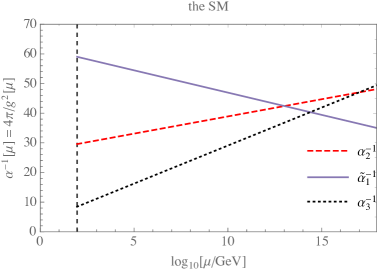
((a))    (a)

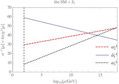
((b))    (b)

Figure 1: Running of the gauge couplings with the particle content of the SM and with the inclusion of $S_{1}$ . The vertical dotted line corresponds to the electroweak scale $M_{Z}$. For $\alpha_{1}^{-1}$, we plot the redefined quantity $\widetilde{\alpha}^{-1}_{1}\equiv\frac{3}{5}\alpha^{-1}_{1}$ as required by the $\mathrm{SO}(10)$ boundary conditions. Including the leptoquark in the particle content does not provide a significant modification to the SM RG running in favour of unification.

III.2 Unification with a single intermediate scale

We start by labelling the energy intervals in between symmetry-breaking scales $[M_{Z},M_{C}]$ and $[M_{C},M_{U}]$ with Roman numerals as

$$\mathrm{I} \;:\; [M_{Z},\;M_{C}],\quad G_{213}\;(\mathrm{SM}),$$ (17)

$$\mathrm{II} \;:\; [M_{C},\;M_{U}],\quad G_{224}\quad\mbox{or}\quad G_{224D}\;.$$ (18)

The boundary/matching conditions we impose on the couplings at the symmetry-breaking scales are

$$M_{U} \;:\; g_{L}(M_{U})\;=\;g_{R}(M_{U})\;=\;g_{4}(M_{U}),\vphantom{\bigg{|}}$$ (19)

$$M_{C} \;:\; g_{3}(M_{C})=g_{4}(M_{C}),\quad g_{2}(M_{C})\;=\;g_{L}(M_{C}),$$

$$\frac{1}{g_{1}^{2}(M_{C})}\;=\;\frac{1}{g_{R}^{2}(M_{C})}+\frac{2}{3}\frac{1}{g_{4}^{2}(M_{C})},$$

$$g_{L}(M_{C})\;=\;g_{R}(M_{C})\mbox{ (absent in the $G_{224}$ case)}\vphantom{\Bigg{|}}$$ (21)

$$M_{Z} \;:\; \frac{1}{e^{2}(M_{Z})}\;=\;\frac{1}{g_{1}^{2}(M_{Z})}+\frac{1}{g_{2}^{2}(M_{Z})}\;.\vphantom{\Bigg{|}}$$ (22)

We use the central values of the low-energy data as the boundary conditions in the RG running (in the $\overline{\mathrm{MS}}$ scheme) Patrignani:2016xqp ; ALEPH:2005ab $\alpha^{-1}=127.95$, $\alpha_{s}=0.118$, $\sin^{2}\theta_{W}=0.2312$ at $M_{Z}=91.2\,\mathrm{GeV}$, which translate to $g_{1}=0.357$, $g_{2}=0.652$, $g_{3}=1.219$. The coupling constants are all required to remain in the perturbative regime during the evolution from $M_{Z}$ to $M_{U}$.

The RG coefficients, $a_{i}$, differ depending on the particle content in each energy interval, changing every time symmetry-breaking occurs. Together with the matching and boundary conditions, one-loop RG running leads to the following conditions on the symmetry-breaking scales $M_{U}$ and $M_{C}$:

$$2\pi\left[\dfrac{3-8\sin^{2}\theta_{W}(M_{Z})}{\alpha(M_{Z})}\right]=\left(3a_{1}-5a_{2}\right)\ln\dfrac{M_{C}}{M_{Z}}\hskip 28.45274pt$$

$$+\left(-5a_{L}+3a_{R}+2a_{4}\right)\ln\dfrac{M_{U}}{M_{C}},$$ (23)

$$2\pi\left[\dfrac{3}{\alpha(M_{Z})}-\dfrac{8}{\alpha_{s}(M_{Z})}\right]=\left(3a_{1}+3a_{2}-8a_{3}\right)\ln\dfrac{M_{C}}{M_{Z}}$$

$$+\left(3a_{L}+3a_{R}-6a_{4}\right)\ln\dfrac{M_{U}}{M_{C}},$$ (25)

where the notation on $a_{i}$ is self-evident. The unified gauge coupling $\alpha_{U}$ at the scale $M_{U}$ is then obtained from

$$\dfrac{2\pi}{\alpha_{U}}=\dfrac{2\pi}{\alpha_{s}(M_{Z})}-\left(a_{4}\;\ln\dfrac{M_{U}}{M_{C}}+a_{3}\;\ln\dfrac{M_{C}}{M_{Z}}\right)\;.\qquad$$ (26)

Thus, once the RG coefficients in each interval are specified, the scales $M_{U}$ and $M_{C}$, and the value of $\alpha_{U}$ are uniquely determined. The results are given in Table 3, and unification of the couplings is displayed in Fig. 2 for each model.

As mentioned previously, we assume in this paper that the proton-decay-mediating couplings of $S_{1}$ are suppressed. On the other hand, we do not make any assumptions regarding the other potentially dangerous operators which could lead to proton decay. Thus, it is necessary to inspect whether the predictions of our models displayed in Table 3 are compatible with the current bounds coming from the proton decay searches or not. The most recent and stringent bound on the lifetime of the proton comes from the mode $p\rightarrow e^{+}\pi^{0}$, and is $\tau_{p}>1.6\times 10^{34}$ years Miura:2016krn . As for the proton decay modes that are mediated by the super-heavy gauge bosons, which reside in the adjoint representation of $\mathrm{SO}(10)$ $\mathbf{45}$, considering that $\tau_{p}\sim M_{U}^{4}/m_{p}^{5}\alpha_{U}^{2}$ Langacker:1980js , we obtain $M_{U}\gtrsim 10^{15.9}$ GeV, which is consistent with predictions of both model $A_{1}$ and model $A_{2}$, within an order of magnitude of the latter. Additionally, since $M_{C}$ is the scale at which the Pati-Salam symmetry breaks into the SM, it determines the expected mass values for the proton-decay-mediating colour triplets. From a naive analysis Altarelli:2013aqa , it can be shown that the current bounds on the proton lifetime require $M_{C}\gtrsim 10^{11}$ GeV, again consistent with the predictions of both model $A_{1}$ and model $A_{2}$, within an order of magnitude of the former. Note that these bounds should be taken as order-of-magnitude estimates since, while obtaining them, we approximate the anticipated masses of the super-heavy gauge bosons and the colour triplets as $M_{X}\approx M_{U}$ and $M_{T}\approx M_{C}$, while it would not be unreasonable to expect that these mass values could differ from the corresponding energy scales within an order of magnitude.

Table 3: The predictions of models $A_{1}$ and $A_{2}$.

Model	$A_{1}$	$A_{2}$
$\log_{10}(M_{U}/\mathrm{GeV})$	$17.1$	$15.6$
$\log_{10}(M_{C}/\mathrm{GeV})$	$10.9$	$13.7$
$\alpha_{U}^{-1}$	$29.6$	$35.4$

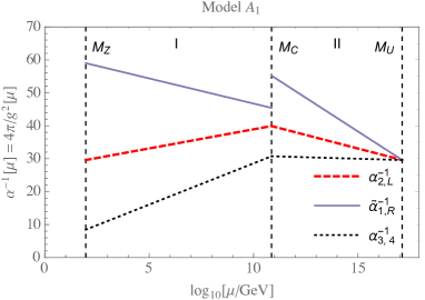
((a))    (a)

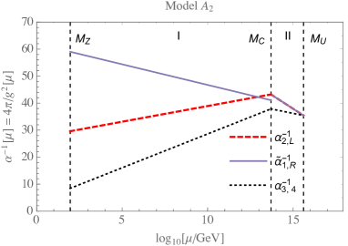
((b))    (b)

Figure 2: Running of the gauge couplings for models $A_{1}$ and $A_{2}$. Note that $\widetilde{\alpha}^{-1}_{1}\equiv\frac{3}{5}\alpha^{-1}_{1}$. The discontinuity at $M_{C}$ in each plot is due to the boundary conditions given in Eq. (22).

IV Low-energy phenomenology

The existence of a TeV scale charge $-1/3$ scalar leptoquark in a GUT framework is quite interesting from a phenomenological perspective mainly for two reasons. First, its existence is testable at the LHC. The direct-detection searches for scalar leptoquarks have been putting exclusion bounds on $S_{1}$ with different decay hypotheses Sirunyan:2018nkj ; Sirunyan:2018kzh . Second, as mentioned earlier, such a leptoquark can offer an explanation of some persistent flavour anomalies observed in several experiments. For example, if we consider the anomalies observed in the $B$-meson semileptonic decays via charged currents (collectively these show the most significant departure from the SM expectations), $S_{1}$ can provide an explanation if it couples with $\tau$ and neutrino(s) and $b$ and $c$ quarks. The direct LHC bounds on such a leptoquark are not very severe but as it has been pointed out in Ref. Mandal:2018kau , the present LHC data in the $pp\to\tau\tau/\tau\nu$ channels have actually put constraints on the $S_{1}$ parameter space relevant for explaining the observed $R_{D^{(*)}}$ anomalies. Here, using flavour data and LHC constraints, we obtain the allowed parameter space in our model. We also point out some possible new search channels at the LHC. On the flavour side, our primary focus is on the charged-current anomalies observed in the semileptonic $B$ decays in the $R_{D^{(*)}}$ observables. Hence, as in Ref. Mandal:2018kau , we focus on the interaction terms of $S_{1}$ that could play a role to address the $R_{D^{(*)}}$ anomalies for simplicity.

IV.1 The ${\mathbf{S}_{1}}$ model

The single TeV scale $S_{1}$ leptoquark that originates from the GUT model discussed in Sec. II transforms under the SM gauge group as $\left(3,1,-1/3\right)$. The low-energy interactions of $S_{1}$ with the SM fields are shown in a compact manner in Eq. (12). Below, we display the relevant interaction terms required for our phenomenological analysis,

$$\mathcal{L}\supset\left[\lambda_{ij}^{L}\bar{Q}^{c}_{i}\left(i\tau_{2}\right)L_{j}+\lambda_{ij}^{R}\bar{u}^{c}_{i}\ell_{Rj}\right]S_{1}^{{\dagger}}+\mathrm{H.c.}\ ,$$ (27)

where $Q_{i}$ and $L_{i}$ denote the $i$th-generation quark and lepton doublets, respectively and $\lambda_{ij}^{H}$ represents the coupling of $S_{1}$ with a charge-conjugate quark of $i$th generation and a lepton of $j$-th generation with chirality $H$. Without any loss of generality, we assume all $\lambda$’s are real in our collider analysis since the LHC data that we consider are insensitive to their complex nature. Also, we only consider mixing among quarks [Cabibbo-Kobayashi-Maskawa (CKM) mixing] and ignore neutrino mixing [Pontecorvo-Maki-Nakagawa-Sakata (PMNS) mixing] completely as all neutrino flavours contribute to the missing energy and hence are not not distinguishable at the LHC. The couplings of $S_{1}$ to the first-generation SM fermions are heavily constrained Cai:2017wry . Hence, we assume $\lambda_{1i},\lambda_{i1}=0$ in our analysis.

((a))    (a)

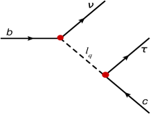
((b))    (b)

((c))    (c)

Figure 3: Leading-order parton-level Feynman diagrams responsible for the $B\to D^{(*)}\tau\nu$ decay (a) in the SM, and (b) in the $S_{1}$ model. The parton-level process in the presence of $S_{1}$ that would contribute to $B\to K\nu\nu$ is shown in diagram (c).

The parton level Feynman diagrams for the $b\to c\tau\nu$ decay (responsible for the $B\to D^{(*)}\tau\nu$ decay) are shown in Fig. 3. In order to have a nonzero contribution in the $R_{D^{(*)}}$ observables from $S_{1}$, we need $b\nu S_{1}$ and $c\tau S_{1}$ couplings to be nonzero simultaneously. Minimally, one can start with just a single free coupling – either $\lambda_{23}^{L}$ or $\lambda_{33}^{L}$. The coupling $\lambda_{23}^{L}$ ($\lambda_{33}^{L}$) directly generates $c\tau S_{1}$ ($b\nu S_{1}$) interaction and the other one, i.e., the $b\nu S_{1}$ ($c\tau S_{1}$) can be generated through the CKM mixing among quarks. These two minimal scenarios were discussed in detail in Ref. Mandal:2018kau . For these two cases, the Lagrangian in Eq. (27) can be written explicitly as,

$$C_{1}:~{}~{}\mathcal{L} \supset\lambda_{23}^{L}\left[\bar{c}^{c}\tau_{L}-\left(V_{cb}\bar{b}^{c}+V_{cs}\bar{s}^{c}+V_{cd}\bar{d}^{c}\right)\nu\right]S_{1}^{{\dagger}}$$

$$+\ \mathrm{H.c.}\quad(\lambda_{33}^{L}=0),$$ (28)

$$C_{2}:~{}~{}\mathcal{L} \supset\lambda_{33}^{L}\left[\left(V^{*}_{ub}\bar{u}^{c}+V^{*}_{cb}\bar{c}^{c}+V^{*}_{tb}\bar{t}^{c}\right)\tau_{L}-\bar{b}^{c}\nu\;\right]S_{1}^{{\dagger}}$$

$$+\ \mathrm{H.c.}\quad(\lambda_{23}^{L}=0).$$ (29)

In Ref. Mandal:2018kau , it was shown that for $C_{1}$, the $R_{D^{(*)}}$-favoured parameter space is already ruled out by the latest LHC data. On the other hand, $C_{2}$ is not seriously constrained by the LHC data since this scenario is insensitive to the coupling $\lambda_{33}^{L}$. Only the pair-production searches, which are largely insensitive to $\lambda_{33}^{L}$, in the $tt\tau\tau$ and $bb\nu\nu$ modes exclude $M_{S_{1}}$ up to 900 GeV Sirunyan:2018nkj and 1100 GeV Sirunyan:2018kzh , respectively for a 100% BR in each decay mode. However, Ref. Bansal:2018nwp showed that the $R_{D^{(*)}}$-favoured parameter space in $C_{2}$ is also ruled out by the electroweak precision data on the $Z\to\tau\tau$ decay.

The above two minimal cases, $C_{1}$ and $C_{2}$, are the two extremes. One can, however, consider a next-to-minimal situation, where both $\lambda_{23}^{L}$ and $\lambda_{33}^{L}$ are nonzero to explain $R_{D^{(*)}}$ anomalies being within the LHC bounds Mandal:2018kau . However, $B\to K^{(*)}\nu\nu$ decay results severely constrain such a scenario due to tree-level leptoquark contribution [see Fig. 3(c)]. References Cai:2017wry ; Angelescu:2018tyl indicated that a large $\lambda_{23}^{R}$ might help explain various flavour anomalies simultaneously while being consistent with other relevant experimental results.

In this paper, we allow $\lambda_{23}^{L}$, $\lambda_{33}^{L}$ and $\lambda_{23}^{R}$ to be nonzero and perform a parameter scan for a single $S_{1}$ solution of the $R_{D^{(*)}}$ anomalies. We locate the $R_{D^{(*)}}$ favoured parameter space that satisfies the limits from $B\to K^{(*)}\nu\nu$ and $Z\to\tau\tau$ decays and is still allowed by the latest LHC data. An $S_{1}$ can also provide new final states at the LHC like $\tau\tau+jets$ and $\tau+\not{E}_{T}+jets$ in which leptoquarks have not been searched for before.

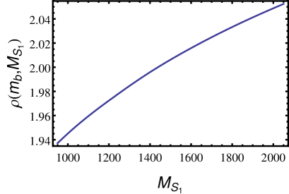
Figure 4: The ratio defined in Eq. (37), $\rho\left(m_{b},M_{S_{1}}\right)=\frac{\mathcal{C}_{S_{L}}}{\mathcal{C}_{T_{L}}}\left(\mu={m_{b}}\right)/\frac{\mathcal{C}_{S_{L}}}{\mathcal{C}_{T_{L}}}\left(\mu=M_{S_{1}}\right)$, obtained from Ref. Cai:2017wry .

Table 4: Summary of the $R_{D^{(*)}}$ related inputs for our parameter scan.

Observable	Experimental Average	SM Expectation	Ratio	Value
$R_{D}$	$0.340\pm 0.027\pm 0.013$ Amhis:2016xyh	$0.299\pm 0.003$ Bigi:2016mdz	$r_{D}$	$1.137\pm 0.101$
$R_{D^{*}}$	$0.295\pm 0.011\pm 0.008$ Amhis:2016xyh	$0.258\pm 0.005$ Amhis:2016xyh	$r_{D^{*}}$	$1.144\pm 0.057$
$F_{L}(D^{*})$	$0.60\pm 0.08\pm 0.035$ Hirose:2016wfn ; Hirose:2017dxl	$0.46\pm 0.04$ Bhattacharya:2018kig	$f_{L}(D^{*})$	$1.313\pm 0.198$
$P_{\tau}(D^{*})$	$-0.38\pm 0.51^{+0.21}_{-0.16}$ Adamczyk:2019wyt	$-0.497\pm 0.013$ Tanaka:2012nw	$p_{\tau}(D^{*})$	$0.766\pm 1.093$

IV.2 ${\mathbf{R}_{D^{(*)}}}$ with ${\mathbf{S}_{1}}$

In the SM, the semitauonic $B$ decay is mediated by the left-handed charged currents and the corresponding four-Fermi interactions are given by the following effective Lagrangian

$$\mathcal{L}_{\rm SM}=-\frac{4G_{F}}{\sqrt{2}}V_{cb}\left[\bar{c}\gamma^{\mu}P_{L}b\right]\left[\bar{\tau}\gamma_{\mu}P_{L}\nu_{\tau}\right]\,.$$ (30)

In the presence of new physics, there are a total five four-Fermi operators that appear in the effective Lagrangian for the $B\to D^{(*)}\tau\nu$ decay Tanaka:2012nw ,

$$\mathcal{L}\supset-\frac{4G_{F}}{\sqrt{2}}V_{cb} \left[\left(1+\mathcal{C}_{V_{L}}\right)\mathcal{O}_{V_{L}}+\mathcal{C}_{V_{R}}\mathcal{O}_{V_{R}}+\mathcal{C}_{S_{L}}\mathcal{O}_{S_{R}}\right.$$

$$\left.+\mathcal{C}_{S_{R}}\mathcal{O}_{S_{R}}+\mathcal{C}_{T_{R}}\mathcal{O}_{T_{R}}\right]\ ,$$ (31)

where the $\mathcal{C}_{X}$’s are the Wilson coefficients associated with the effective operators:

• Vector operators:

  $$\begin{array}[]{ccc}\mathcal{O}_{V_{L}}&=&\left[\bar{c}\gamma^{\mu}P_{L}b\right]\left[\bar{\tau}\gamma_{\mu}P_{L}\nu\right],\\ \mathcal{O}_{V_{R}}&=&\left[\bar{c}\gamma^{\mu}P_{R}b\right]\left[\bar{\tau}\gamma_{\mu}P_{L}\nu\right].\end{array}$$

• Scalar operators:

  $$\begin{array}[]{cccc}\mathcal{O}_{S_{L}}&=&\left[\bar{c}P_{L}b\right]\left[\bar{\tau}P_{L}\nu\right],&\\ \mathcal{O}_{S_{R}}&=&\left[\bar{c}P_{R}b\right]\left[\bar{\tau}P_{L}\nu\right].&\end{array}$$

• Tensor operator:

  $$\begin{array}[]{ccc}\mathcal{O}_{T_{L}}&=&\left[\bar{c}\sigma^{\mu\nu}P_{L}b\right]\left[\bar{\tau}\sigma_{\mu\nu}P_{L}\nu\right].\end{array}$$

The operator $\mathcal{O}_{V_{L}}$ is SM-like and the other four operators introduce new Lorentz structures into the Lagrangian. Note that the operator $\mathcal{O}_{T_{R}}$ is identically zero, i.e.,

$$\mathcal{O}_{T_{R}}=\left[\bar{c}\sigma^{\mu\nu}P_{R}b\right]\left[\bar{\tau}\sigma_{\mu\nu}P_{L}\nu\right]=0.$$ (32)

The $S_{1}$ leptoquark that we consider can generate only $\mathcal{O}_{V_{L},S_{L},T_{L}}$. Hence, the coefficients of the other two operators, namely, $\mathcal{C}_{V_{R}}$ and $\mathcal{C}_{S_{R}}$ remain zero in our model. In terms of the $S_{1}$ parameters the Wilson coefficients can be expressed as,

$$\left.\begin{array}[]{ll}\mathcal{C}_{V_{L}}&=\displaystyle\frac{1}{2\sqrt{2}G_{F}V_{cb}}\frac{\lambda_{23}^{L*}\lambda_{33}^{L}}{2M_{S_{1}}^{2}}\,,\\ \mathcal{C}_{S_{L}}&=\displaystyle-\frac{1}{2\sqrt{2}G_{F}V_{cb}}\frac{\lambda_{33}^{L}\lambda_{23}^{R}}{2M_{S_{1}}^{2}}\,,\\ \mathcal{C}_{T_{L}}&=\displaystyle-\frac{1}{4}\mathcal{C}_{S_{L}}\,.\end{array}\right\}$$ (36)

These relations are obtained at the mass scale $M_{S_{1}}$. However, running of the strong coupling constant down to $m_{b}\sim 4.2$ GeV changes these coefficients substantially except for $\mathcal{C}_{V_{L}}$ which is protected by the QCD Ward identity. As a result, the ratio $\mathcal{C}_{S_{L}}/\mathcal{C}_{T_{L}}$ becomes,

$$\left.\frac{\mathcal{C}_{S_{L}}}{\mathcal{C}_{T_{L}}}\right|_{m_{b}}=\rho\left(m_{b},M_{S_{1}}\right)\left.\frac{\mathcal{C}_{S_{L}}}{\mathcal{C}_{T_{L}}}\right|_{M_{S_{1}}}=-4\rho\left(m_{b},M_{S_{1}}\right).$$ (37)

The modification factor $\rho$ can be obtained from Ref. Cai:2017wry , and we display it in Fig. 4. In terms of the nonzero Wilson coefficients we can express the ratios $r_{D^{(*)}}=R_{D^{(*)}}/R_{D^{(*)}}^{\mathrm{SM}}$ as Iguro:2018vqb ,

$$r_{D}\equiv\frac{R_{D}}{R_{D}^{\mathrm{SM}}}\approx \ |1+\mathcal{C}_{V_{L}}|^{2}+1.02\ |\mathcal{C}_{S_{L}}|^{2}+0.9\ |\mathcal{C}_{T_{L}}|^{2}$$

$$+1.49\ \textrm{Re}\left[(1+\mathcal{C}_{V_{L}})\mathcal{C}_{S_{L}}^{*}\right]$$

$$+1.14\ \textrm{Re}\left[(1+\mathcal{C}_{V_{L}})\mathcal{C}_{T_{L}}^{*}\right],$$ (38)

$$r_{D^{*}}\equiv\frac{R_{D^{*}}}{R_{D}^{\mathrm{SM}}}\approx \ |1+\mathcal{C}_{V_{L}}|^{2}+0.04\ |\mathcal{C}_{S_{L}}|^{2}+16.07\ |\mathcal{C}_{T_{L}}|^{2}$$

$$-0.11\ \textrm{Re}\left[(1+\mathcal{C}_{V_{L}})\mathcal{C}_{S_{L}}^{*}\right]$$

$$-5.12\ \textrm{Re}\left[(1+\mathcal{C}_{V_{L}})\mathcal{C}_{T_{L}}^{*}\right].$$ (39)

With Eq. (37) one can simplify the above equations as,

$$r_{D}= \ |1+\mathcal{C}_{V_{L}}|^{2}+\left(1.02+\frac{0.9}{16\rho^{2}}\right)|\mathcal{C}_{S_{L}}|^{2}$$

$$+\left(1.49-\frac{1.14}{4\rho}\right)\textrm{Re}\left[(1+\mathcal{C}_{V_{L}})\mathcal{C}_{S_{L}}^{*}\right],$$ (40)

$$r_{D^{*}}= \ |1+\mathcal{C}_{V_{L}}|^{2}+\left(0.04+\frac{16.07}{16\rho^{2}}\right)|\mathcal{C}_{S_{L}}|^{2}$$

$$-\left(0.11-\frac{5.12}{4\rho}\right)\textrm{Re}\left[(1+\mathcal{C}_{V_{L}})\mathcal{C}_{S_{L}}^{*}\right],$$ (41)

where $\rho=\rho\left(m_{b},M_{S_{1}}\right)$. There are two other observables related to the $R_{D^{*}}$–the longitudinal $D^{*}$ polarization $F_{L}(D^{*})$ and the longitudinal $\tau$ polarization asymmetry $P_{\tau}(D^{*})$–have recently been measured by the Belle Collaboration Adamczyk:2019wyt ; Hirose:2016wfn ; Hirose:2017dxl . In terms of the nonzero Wilson coefficients in our model, $F_{L}(D^{*})$ and $P_{\tau}(D^{*})$ are expressed as Iguro:2018vqb ,

$$f_{L}(D^{*})\equiv \frac{F_{L}(D^{*})}{F_{L}^{\textrm{SM}}(D^{*})}\approx\ \frac{1}{r_{D^{*}}}\Big{\{}|1+\mathcal{C}_{V_{L}}|^{2}+0.08\ |\mathcal{C}_{S_{L}}|^{2}$$

$$+7.02\ |\mathcal{C}_{T_{L}}|^{2}-0.24\ \textrm{Re}\left[(1+\mathcal{C}_{V_{L}})\mathcal{C}_{S_{L}}^{*}\right]$$

$$-4.37\ \textrm{Re}\left[(1+\mathcal{C}_{V_{L}})\mathcal{C}_{T_{L}}^{*}\right]\Big{\}},$$ (42)

$$p_{\tau}(D^{*})\equiv \frac{P_{\tau}(D^{*})}{P_{\tau}^{\textrm{SM}}(D^{*})}\approx\ \frac{1}{r_{D^{*}}}\Big{\{}|1+\mathcal{C}_{V_{L}}|^{2}-0.07\ |\mathcal{C}_{S_{L}}|^{2}$$

$$-1.86\times|\mathcal{C}_{T_{L}}|^{2}+0.22\ \textrm{Re}\left[(1+\mathcal{C}_{V_{L}})\mathcal{C}_{S_{L}}^{*}\right]$$

$$-3.37\ \textrm{Re}\left[(1+\mathcal{C}_{V_{L}})\mathcal{C}_{T_{L}}^{*}\right]\Big{\}}.$$ (43)

These equations can further be simplified as,

$$f_{L}(D^{*})= \ \frac{1}{r_{D^{*}}}\Big{\{}|1+\mathcal{C}_{V_{L}}|^{2}+\left(0.08+\frac{7.02}{16\rho^{2}}\right)|\mathcal{C}_{S_{L}}|^{2}$$

$$-\left(0.24-\frac{4.37}{4\rho}\right)\textrm{Re}\left[(1+\mathcal{C}_{V_{L}})\mathcal{C}_{S_{L}}^{*}\right]\Big{\}},$$ (44)

$$p_{\tau}(D^{*})= \ \frac{1}{r_{D^{*}}}\Big{\{}|1+\mathcal{C}_{V_{L}}|^{2}-\left(0.07+\frac{1.86}{16\rho^{2}}\right)|\mathcal{C}_{S_{L}}|^{2}$$

$$+\left(0.22+\frac{3.37}{4\rho}\right)\textrm{Re}\left[(1+\mathcal{C}_{V_{L}})\mathcal{C}_{S_{L}}^{*}\right]\Big{\}}.$$ (45)

These two observables have the power to discriminate between new physics models with different Lorentz structures (see e.g. Ref. Blanke:2018yud ). In Table 4, we list the bounds on the $R_{D^{(*)}}$ related observables that we include in our parameter scan.

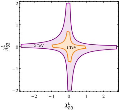
Figure 5: The region where $R_{K^{*}}^{\nu\nu}<2.7$ for $M_{S_{1}}=1$ and $2$ TeV.

IV.3 Constraint from ${\mathbf{R}_{K^{(*)}}^{\nu\nu}}$

The SM flavour-changing neutral-current $b\to s\bar{\nu}\nu$ transition proceeds through a loop and is suppressed by the Glashow-Iliopoulos-Maiani mechanism, whereas in our model, $S_{1}$ can mediate this transition at the tree level [see Fig. 3(c)]. Therefore, this neutral-current decay can heavily constrain the parameter space of our model. We define the following ratio:

$$R_{K^{(*)}}^{\nu\nu}=\frac{\Gamma(B\to K^{(*)}\nu\nu)}{\Gamma(B\to K^{(*)}\nu\nu)_{\mathrm{SM}}}.$$ (46)

The current experimental 90% confidence limit (C.L.) upper limits on the above quantities are $R_{K}^{\nu\nu}<3.9$ and $R_{K^{*}}^{\nu\nu}<2.7$ Grygier:2017tzo . In terms of our model parameters, $R_{K^{(*)}}^{\nu\nu}$ is given by the following expression,

$$R_{K^{(*)}}^{\nu\nu}=1-\frac{2a}{3M_{S_{1}}^{2}}\mathrm{Re}\left(\frac{\lambda_{23}^{L*}\lambda_{33}^{L}}{V_{tb}V_{ts}^{*}}\right)+\frac{a^{2}}{3M_{S_{1}}^{4}}\left|\frac{\lambda_{23}^{L*}\lambda_{33}^{L}}{V_{tb}V_{ts}^{*}}\right|^{2},$$ (47)

where $a=\sqrt{2}\pi^{2}/\left(e^{2}G_{F}|C_{L}^{\mathrm{SM}}|\right)$ with $C_{L}^{\mathrm{SM}}\approx-6.38$ Cai:2017wry . We use this constraint in our analysis and find that it significantly restricts our parameter space. Note that this constraint applies on $\lambda_{23}^{L}$ and $\lambda_{33}^{L}$ but not on $\lambda_{23}^{R}$. In Fig. 5, we show the regions in the $\lambda_{23}^{L}$-$\lambda_{33}^{L}$ plane with $R_{K^{*}}^{\nu\nu}<2.7$ for two different values of $M_{S_{1}}$.

IV.4 Constraint from $\mathbf{Z}\to\tau\tau$ decay

Another important constraint comes from the $Z\tau\tau$ coupling measurements. The $Z\to\tau\tau$ decay is affected by the $S_{1}$ loops as shown in Ref. Bansal:2018nwp . The contribution of $S_{1}$ to the $Z\tau\tau$ coupling shift ($\Delta\kappa_{Z\tau\tau}$) comes from a loop with an up-type quark ($q$) and an $S_{1}$. The shift scales as the square of the $S_{1}t\tau$ coupling ($\lambda^{L/R}_{q3}$) and $m_{q}^{2}$. Hence, the dominant contribution comes from when $q$ is the top quark implying that the $Z\tau\tau$ coupling measurements can restrict only $\lambda_{33}^{L}$ but not $\lambda_{23}^{L}$ or $\lambda_{23}^{R}$. For instance, we see from Ref. Bansal:2018nwp that $\lambda_{33}^{L}\gtrsim 1.4$ can be excluded for $M_{S_{1}}\sim 1$ TeV with $2\sigma$ confidence. We incorporate this bound into our parameter scan.

IV.5 LHC phenomenology and constraints

We now make a quick survey of the relevant LHC phenomenology of a TeV-range $S_{1}$ that couples with $\tau$, $\nu$ and $s$ and $c$ quarks. For this discussion we compute all the necessary cross sections using the universal FeynRules output (UFO)  Degrande:2011ua model files from Ref. Mandal:2018kau in MadGraph5 Alwall:2014hca . We use the NNPDF23LO Ball:2012cx parton distribution functions (PDFs). Wherever required, we include the next-to-leading-order QCD $K$-factor of $\sim 1.3$ for the pair production in our analysis Mandal:2015lca .

IV.5.1 Decay modes of $S_{1}$

For nonzero $\lambda_{23}^{L}$, $\lambda_{33}^{L}$ and $\lambda_{23}^{R}$, $S_{1}$ can decay to $c\tau$, $s\nu$, $t\tau$ and $b\nu$ states. CKM mixing among quarks enables decays to $u\tau$ and $d\nu$ but we neglect them in our analysis as the off-diagonal CKM elements are small. The BRs of $S_{1}$ to various decay modes vary depending on the coupling strengths. If $\lambda_{23}^{R}\gg\lambda_{23}^{L},\lambda_{33}^{L}$, the dominant decay mode is $S_{1}\to c\tau$, whereas for $\lambda_{23}^{L}\gg\lambda_{23}^{R},\lambda_{33}^{L}$, $\mathrm{BR}(S_{1}\to c\tau)\approx\mathrm{BR}(S_{1}\to s\nu)\approx 50\%$. On the other hand, when $\lambda_{33}^{L}\gg\lambda_{23}^{L},\lambda_{23}^{R}$, the dominant decay modes are $S_{1}\to t\tau$ and $S_{1}\to b\nu$ with about 50% BR in each mode. Since partial decay widths depend linearly on $M_{S_{1}}$, BRs are insensitive to the mass of $S_{1}$.

IV.5.2 Production of $S_{1}$

At the LHC, $S_{1}$ can be produced resonantly in pairs or singly and nonresonantly through indirect production ($t$-channel $S_{1}$ exchange process).

Pair production: The pair production of $S_{1}$ is dominated by the strong coupling and, therefore, it is almost model independent. The mild model dependence enters in the pair production through the $t$-channel lepton or neutrino exchange processes. However, the amplitudes of those diagrams are proportional to $\lambda^{2}$ and generally suppressed for small $\lambda$ values (for bigger $M_{S_{1}}$ and large $\lambda$ values, this part could be comparable to the model independent part of the pair production). Pair production is heavily phase-space suppressed for large $M_{S_{1}}$ and we find that its contribution is very small in our recast analysis. Pair production can be categorized into two types depending on the final states: symmetric, where both leptoquarks decay to the same modes, asymmetric, where the two leptoquarks decay via two different modes. These two types give rise to various novel final states.

Symmetric modes:

$$S_{1}S_{1}\to c\tau\raisebox{6.78123pt}{$\frown$}\ c\tau\raisebox{6.78123pt}{$\frown$}\equiv\tau\tau+2j,\quad t\tau\raisebox{6.78123pt}{$\frown$}\ t\tau\raisebox{6.78123pt}{$\frown$}\equiv tt+\tau\tau,\quad s\nu\raisebox{6.78123pt}{$\frown$}\ s\nu\raisebox{6.78123pt}{$\frown$}\equiv 2j+\not{E}_{\rm T},\quad b\nu\raisebox{6.78123pt}{$\frown$}\ b\nu\raisebox{6.78123pt}{$\frown$}\equiv 2b+\not{E}_{\rm T}.$$

Asymmetric modes:

$$S_{1}S_{1} \to c\tau\raisebox{6.78123pt}{$\frown$}\ s\nu\raisebox{6.78123pt}{$\frown$}\equiv\tau+2j+\not{E}_{\rm T},\quad c\tau\raisebox{6.78123pt}{$\frown$}\ b\nu\raisebox{6.78123pt}{$\frown$}\equiv\tau+b+j+\not{E}_{\rm T},\quad c\tau\raisebox{6.78123pt}{$\frown$}\ t\tau\raisebox{6.78123pt}{$\frown$}\equiv\tau\tau+t+j,$$

$$S_{1}S_{1} \to s\nu\raisebox{6.78123pt}{$\frown$}\ b\nu\raisebox{6.78123pt}{$\frown$}\equiv b+j+\not{E}_{\rm T},\quad s\nu\raisebox{6.78123pt}{$\frown$}\ t\tau\raisebox{6.78123pt}{$\frown$}\equiv t+\tau+j+\not{E}_{\rm T},\quad b\nu\raisebox{6.78123pt}{$\frown$}\ t\tau\raisebox{6.78123pt}{$\frown$}\equiv t+\tau+b+\not{E}_{\rm T},$$

where the curved connection over a pair of particles indicates that the pair is coming from a decay of $S_{1}$. Searches for leptoquarks in some of the symmetric modes were already done at the LHC Sirunyan:2018nkj ; Sirunyan:2018kzh . Leptoquark searches in some of the symmetric and most of the asymmetric modes are yet to be performed at the LHC.

Single production: The single productions of $S_{1}$, where $S_{1}$ is produced in association with a SM particle, are fully model dependent as they depend on the leptoquark-quark-lepton couplings. These are important production modes for large couplings and heavier masses (since single productions receive less phase-space suppression than the pair production). Depending on the final states, single productions can be categorized as follows.

Symmetric modes:

$$\mathcal{S}_{1}\ \tau\ X \to\ \tau c\raisebox{6.78123pt}{$\frown$}\ \tau\ +\ \tau c\raisebox{6.78123pt}{$\frown$}\ \tau\ j \ (+\ \tau c\raisebox{6.78123pt}{$\frown$}\ \tau\ jj\ +\ \cdots)\ \equiv\ \tau\tau+jets$$

$$\mathcal{S}_{1}\ \tau\ X \to\ \tau t\raisebox{6.78123pt}{$\frown$}\ \tau\ +\ \tau t\raisebox{6.78123pt}{$\frown$}\ \tau\ j \ (+\ \tau t\raisebox{6.78123pt}{$\frown$}\ \tau\ jj\ +\ \cdots)\ \equiv\ \tau\tau+t+jets$$

$$\mathcal{S}_{1}\ \nu\ X \to\ \nu s\raisebox{6.78123pt}{$\frown$}\ \nu\ +\ \nu s\raisebox{6.78123pt}{$\frown$}\ \nu\ j \ (+\ \nu s\raisebox{6.78123pt}{$\frown$}\ \nu\ jj\ +\ \cdots)\ \equiv\ \not{E}_{\rm T}+jets$$

$$\mathcal{S}_{1}\ \nu\ X \to\ \nu b\raisebox{6.78123pt}{$\frown$}\ \nu\ +\ \nu b\raisebox{6.78123pt}{$\frown$}\ \nu\ j \ (+\ \nu b\raisebox{6.78123pt}{$\frown$}\ \nu\ jj\ +\ \cdots)\ \equiv\ \not{E}_{\rm T}+b+jets$$

Asymmetric modes:

$$S_{1}\ \tau\ X \to\ \nu s\raisebox{6.78123pt}{$\frown$}\ \tau\ +\ \nu s\raisebox{6.78123pt}{$\frown$}\ \tau\ j \ (+\ \nu s\raisebox{6.78123pt}{$\frown$}\ \tau\ jj\ +\ \cdots)\ \equiv\ \not{E}_{\rm T}+\tau+jets$$

$$S_{1}\ \nu\ X \to\ \tau c\raisebox{6.78123pt}{$\frown$}\ \nu\ +\ \tau c\raisebox{6.78123pt}{$\frown$}\ \nu\ j \ (+\ \tau c\raisebox{6.78123pt}{$\frown$}\ \nu\ jj\ +\ \cdots)\ \equiv\ \not{E}_{\rm T}+\tau+jets$$

$$S_{1}\ \tau\ X \to\ \nu b\raisebox{6.78123pt}{$\frown$}\ \tau\ +\ \nu b\raisebox{6.78123pt}{$\frown$}\ \tau\ j \ (+\ \nu b\raisebox{6.78123pt}{$\frown$}\ \tau\ jj\ +\ \cdots)\ \equiv\ \not{E}_{\rm T}+\tau+b+jets$$

$$S_{1}\ \nu\ X \to\ \tau t\raisebox{6.78123pt}{$\frown$}\ \nu\ +\ \tau t\raisebox{6.78123pt}{$\frown$}\ \nu\ j \ (+\ \tau t\raisebox{6.78123pt}{$\frown$}\ \nu\ jj\ +\ \cdots)\ \equiv\ \not{E}_{\rm T}+\tau+t+jets$$

Here $j$ stands for an untagged jet and $jets$ means any number ($\geq 1$) of untagged jets. These extra jets can be either radiation or hard (genuine three-body single production processes can have sizeable cross sections; see Refs. Mandal:2012rx ; Mandal:2015vfa ; Mandal:2016csb for how one can systematically compute them). As single production is model dependent, the relative strengths of these modes depend on the relative strengths of the coupling involved in the production as well as the BR of the decay mode involved.

Indirect production: Indirect production is the nonresonant process where a leptoquark is exchanged in the $t$ channel. With leptoquark couplings to $\tau$ and $\nu$, this basically gives rise to three possible final states: $\tau\tau~{}(\tau\tau+jets)$, $\tau\nu~{}(\not{E}_{\rm T}+\tau+jets)$ and $\nu\nu~{}(\not{E}_{\rm T}+jets)$. The amplitudes of these processes are proportional to $\lambda^{2}$. So the cross section grows as $\lambda^{4}$. Hence, for an order-one $\lambda$, indirect production has a larger cross section than other production processes for large $M_{S_{1}}$ (see Fig. 2 of Ref. Mandal:2018kau ). However, the indirect production substantially interferes with the SM background process $pp\to V^{(*)}\to\ell\ell$ ($\ell=\tau/\nu$). Though the interference is $\mathcal{O}(\lambda^{2})$, its contribution can be significant for a TeV-scale $S_{1}$ because of the large SM contribution (larger than both the direct production modes and the $\lambda^{4}$ indirect contribution, assuming $\lambda\gtrsim 1$). In general, the interference could be either constructive or destructive depending on the nature of the leptoquark species and its mass Bansal:2018eha . For $S_{1}$, we find that the interference is destructive in nature Mandal:2018kau . Hence, for a TeV-scale $S_{1}$ if $\lambda$ is large, this destructive interference becomes its dominant signature in the leptonic final states.

IV.5.3 Constraints from the LHC

The mass exclusion limits from the pair-production searches for $S_{1}$ at the LHC are as follows. Assuming a $100\%$ BR in the $S\to t\tau$ mode, a recent search at the CMS detector has excluded masses below $900$ GeV Sirunyan:2018nkj . Similarly, for a leptoquark that decays exclusively to $b\nu$ or $s\nu~{}(\equiv j\nu$) final states, the exclusion limits are at $1100$ and $980$ GeV Sirunyan:2018kzh , respectively. However, going beyond simple mass exclusions, we make use of the analysis done in Ref. Mandal:2018kau for the LHC constraints. It contains the independent LHC limits on the three couplings shown in Eq. (27) as functions of $M_{S_{1}}$ as well as a summery of the direct-detection exclusion limits.

Apart from the processes with $\not{E}_{\rm T}+jets$ final states, all other production processes can have either $\tau\tau+jets$ final states or $\not{E}_{\rm T}+\tau+jets$ final states. Hence, the latest $pp\to Z^{\prime}\to\tau\tau$ and $pp\to W^{\prime}\to\tau\nu$ searches at the ATLAS detector Aaboud:2017sjh ; Aaboud:2018vgh were used to derive the constraints in Ref. Mandal:2018kau . There we notice that the limits on $\lambda^{L}_{23}$ from the $\tau\nu$ data are weaker that the ones obtained from the $\tau\tau$ data. The $\tau\tau$ data also constrain $\lambda^{R}_{23}$. From the earlier discussion, it is clear that the interference contribution plays the dominant role in determining these limits. However, its destructive nature means that in the signal region one would expect less events than the SM-only predictions. Hence, the limits were obtained assuming that either $\lambda^{L}_{23}$ or $\lambda^{R}_{23}$ is nonzero at a time or by performing a $\chi^{2}$ test of the transverse mass ($m_{\rm T}$) distributions of the data. As, for heavy $S_{1}$, the limits on $\lambda^{L}_{23}$ and $\lambda^{R}_{23}$ are dominantly determined by the interference of the indirect production, they are very similar. We can translate these limits from the $\tau\tau$ data on any combination of $\lambda^{L}_{23}$ and $\lambda^{R}_{23}$ in a simple manner assuming $\lambda^{L/R}_{23}=\sqrt{\left(\lambda_{23}^{L}\right)^{2}+\left(\lambda_{23}^{R}\right)^{2}}$. In Fig. 6 we display the limits on $\lambda^{L/R}_{23}$ as a function of $M_{S_{1}}$.

The LHC data is insensitive to $\lambda^{L}_{33}$ as it was shown in Ref. Mandal:2018kau . This can be understood from the following argument. First, the pair production is insensitive to this coupling as we have already mentioned. Second, the single-production process $pp\to t\tau\nu$ via an $S_{1}$ has too small a cross section ($\sim 2$ fb for $\lambda^{L}_{33}\sim 1$ and $M_{S_{1}}=1$ TeV) to make any difference at the present luminosity. Finally, there is no interference contribution in the $\tau\tau$ and $\tau+\not{E}_{\rm T}$ channels as there is no $t$ quark in the initial state. Hence, $\lambda^{L}_{33}$ remains unbounded from these searches.

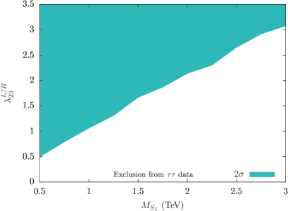
Figure 6: Two-sigma exclusion limits on $\lambda^{L/R}_{23}=\sqrt{\left(\lambda_{23}^{L}\right)^{2}+\left(\lambda_{23}^{R}\right)^{2}}$ as a function of $M_{S_{1}}$ as obtained in Ref. Mandal:2018kau from the ATLAS $pp\to\tau\tau$ data Aaboud:2017sjh . The coloured region is excluded.

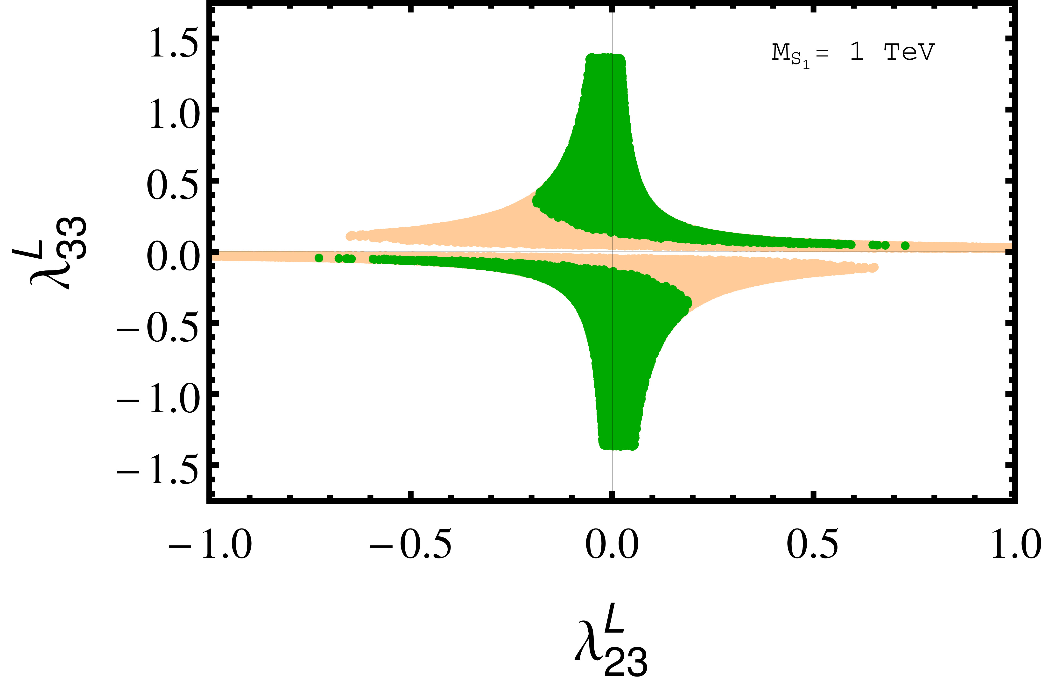
((a))    (a)

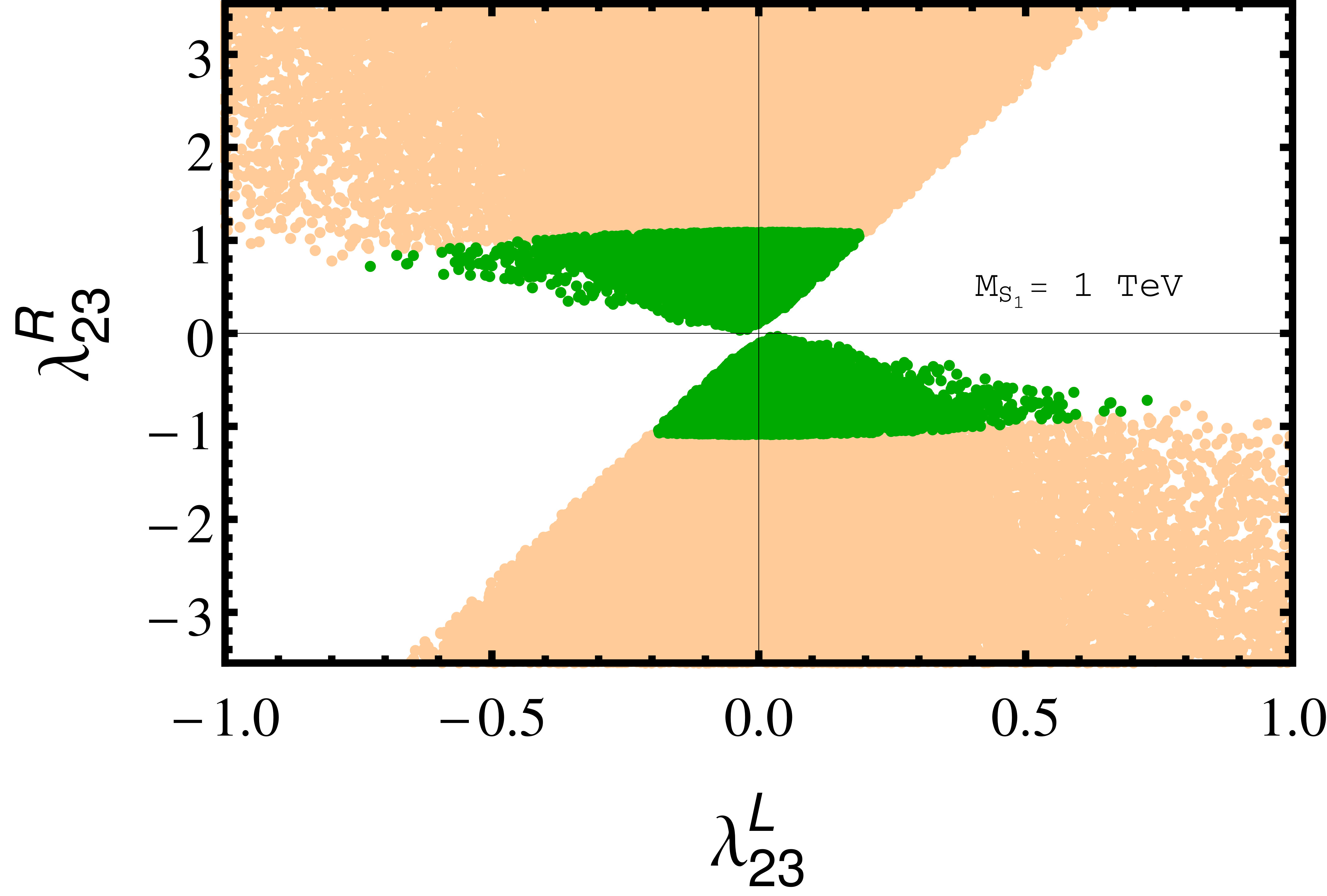
((b))    (b)

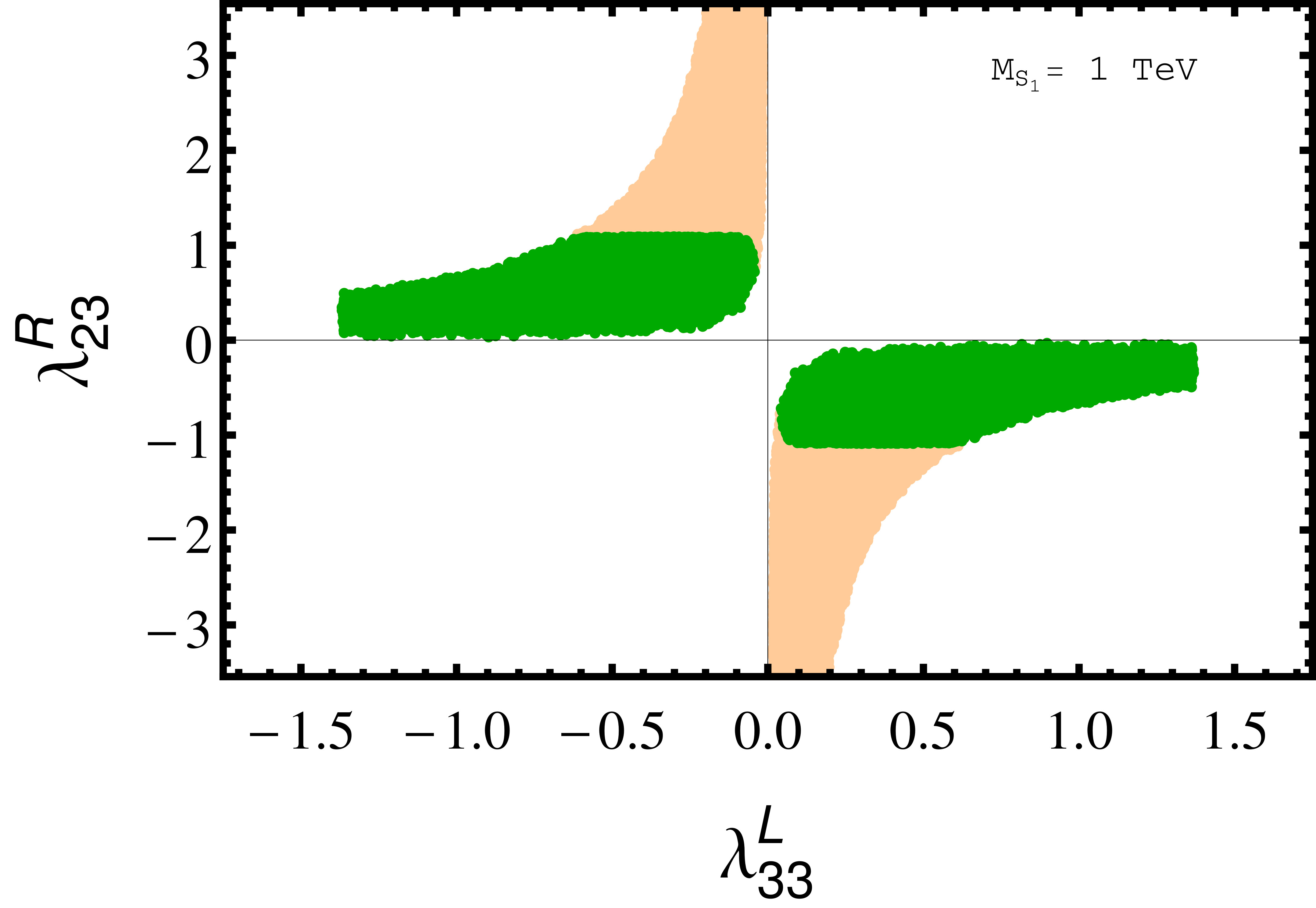
((c))    (c)

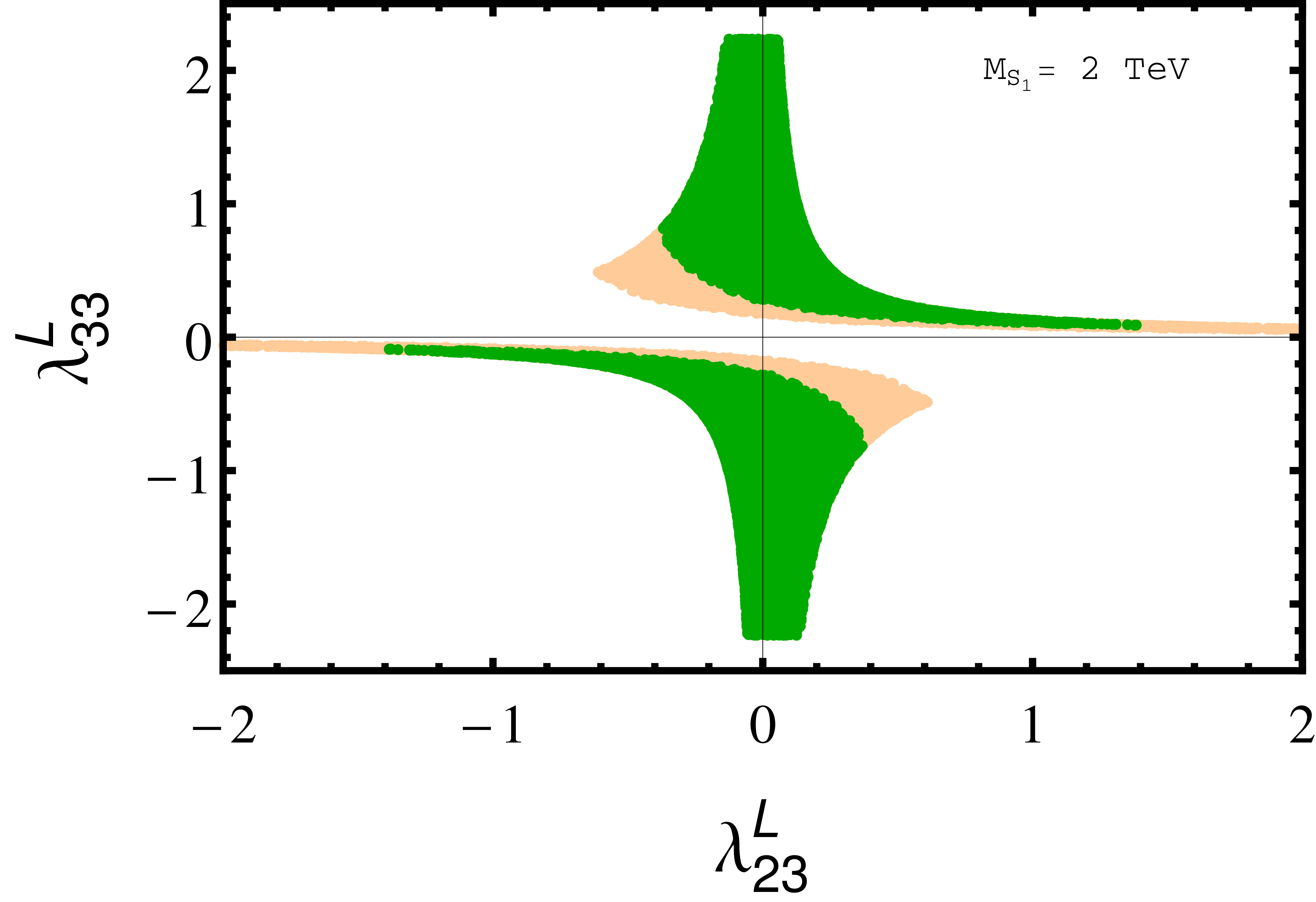
((d))    (d)

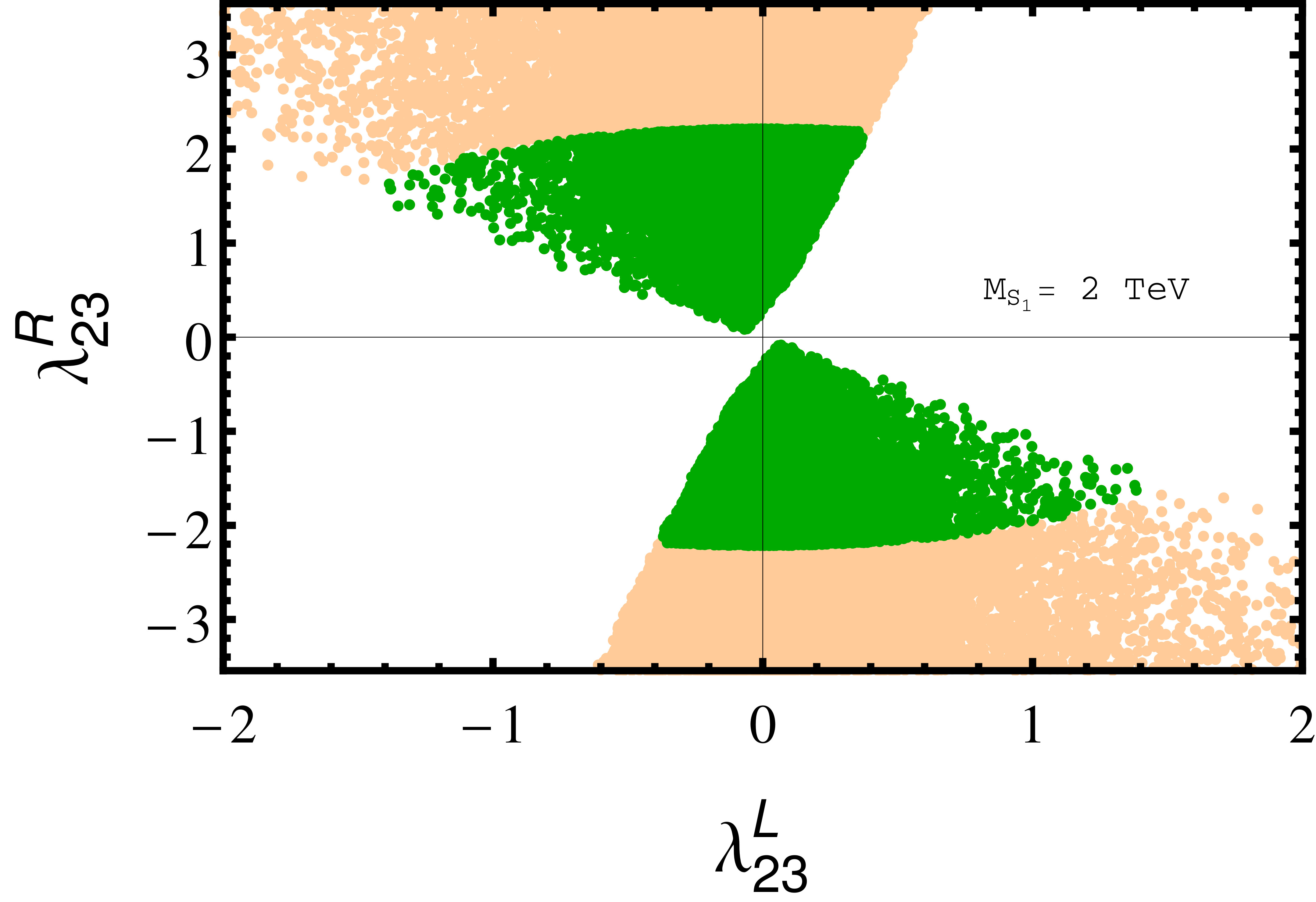
((e))    (e)

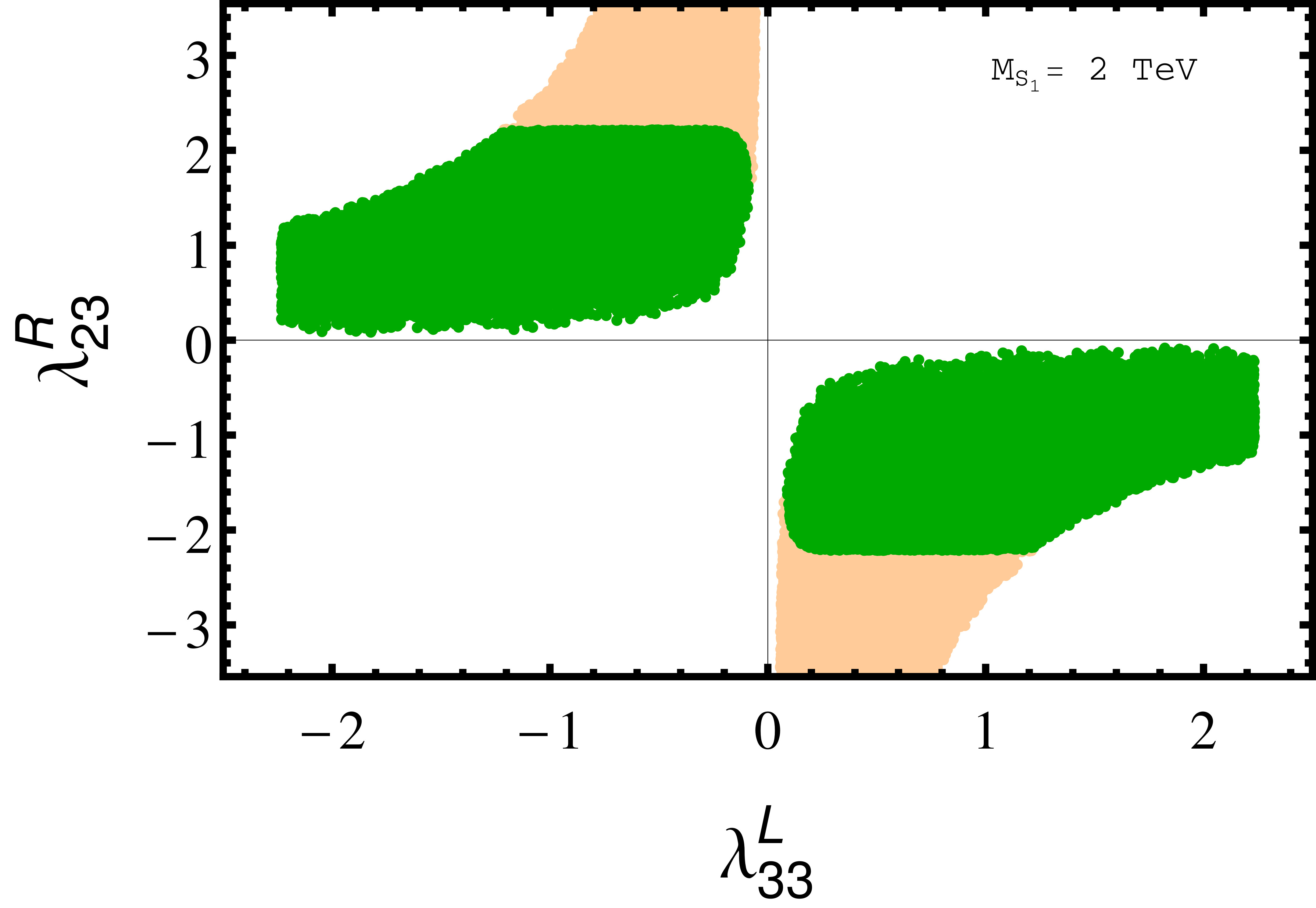
((f))    (f)

Figure 7: Two-dimensional projections of the regions in the $S_{1}$ parameter space allowed by the bounds on the $R_{D^{(*)}}$, $F_{L}(D^{*})$, $P_{\tau}(D^{*})$ and $R^{\nu\nu}_{K^{(*)}}$ observables and the $Z\to\tau\tau$ decay, i.e., the FEW regions (orange), see Sec. IV.6, and the LHC constraints in addition to all these constraints, i.e., the FEWL regions (green) for $M_{S_{1}}=1$ TeV (upper panel) and $M_{S_{1}}=2$ TeV (lower panel). We assume all the couplings are real.

IV.6 Parameter scan

To find the $R_{D^{(*)}}$-favoured regions in the $S_{1}$ parameter space that is not in conflict with the limits on $F_{L}(D^{*})$, $P_{\tau}(D^{*})$, $R^{\nu\nu}_{K^{(*)}}$, $Z\to\tau\tau$ decay and the bounds from the LHC, we consider two benchmark leptoquark masses, $M_{S_{1}}=1$ and $2$ TeV. We allow all the three free couplings, $\lambda_{23}^{L}$, $\lambda_{23}^{R}$ and $\lambda_{33}^{L}$ to vary. For every benchmark mass, we perform a random scan over the three couplings in the perturbative range $-\sqrt{4\pi}$ to $\sqrt{4\pi}$ (i.e., $|\lambda|^{2}/4\pi\leq 1$). We do not consider complex values for the couplings. In Fig. 7, we show the outcome of our scan with different two-dimensional projections. In every plot we show two couplings and allow the third coupling to vary. In each of these plots we show the following.

• The Flavour ${\bm{\cup}}$ EW (FEW) regions: The orange dots mark the regions favoured by the $R_{D^{(*)}}$ observables within $95$% C.L. while satisfying the available bounds on the $F_{L}(D^{*})$, $P_{\tau}(D^{*})$ and $R^{\nu\nu}_{K^{(*)}}$ observables (flavour bounds). In addition, these points also satisfy the bound on $\lambda^{L}_{33}$ coming from the $Z\to\tau\tau$ decay within $95$% C.L. Bansal:2018nwp (electroweak bound).

• The Flavour ${\bm{\cup}}$ EW ${\bm{\cup}}$ LHC (FEWL) regions: As we take into account the limits on $\lambda^{L/R}_{23}$ from the ATLAS $pp\to\tau\tau$ data from the $13$ TeV LHC Mandal:2018kau along with the previous constraints we obtain the regions marked by the green points. These are the points that survive all the limits considered in this paper.

From the plots we see that substantial portions of parameter regions survive after all the constraints. This implies that the $S_{1}$ model can successfully explain the $R_{D^{(*)}}$ anomalies. If one looks only at the $R_{D^{(*)}}$ anomalies, in principle, one can just set $\lambda^{L}_{23}$ and/or $\lambda^{L}_{33}$ to be large. But coupling values that make $C_{V_{L}}$ [see Eq. (36)] big come into conflict with the $R_{K^{(*)}}^{\nu\nu}$ bound [see Eq. (47)]. This is why we do not see any point where both $\lambda^{L}_{23}$ and $\lambda^{L}_{33}$ are large in the first column of Fig. 7. In addition, the LHC puts bounds on $\lambda^{L/R}_{23}$ Mandal:2018kau whereas the $Z\to\tau\tau$ data puts a complimentary bound on $\lambda^{L}_{33}$ Bansal:2018nwp . The restriction on $\lambda^{L}_{33}$ from the $Z\to\tau\tau$ data can be seen in Figs. 7(a) and 7(c) for $M_{S_{1}}=1$ TeV and Figs. 7(d) and 7(f) for $M_{S_{1}}=2$ TeV, whereas from the middle column [i.e., Figs. 7(b) and 7(e)] it is clear that the LHC prevents both $\lambda^{L}_{23}$ and $\lambda^{R}_{23}$ from taking large values simultaneously. From the $\lambda^{R}_{23}$ vs $\lambda^{L}_{33}$ plots [Figs. 7(c) and 7(f)] we see that these two couplings take opposite signs mainly because both $R_{D^{*}}$ and $F_{L}\left(D^{*}\right)$ prefer a positive $C_{S_{L}}$ [see Eqs. (41) and (44)].

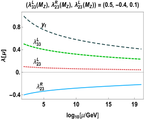
((a))    (a)

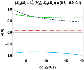
((b))    (b)

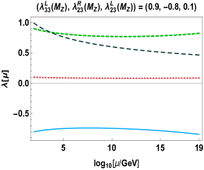
((c))    (c)

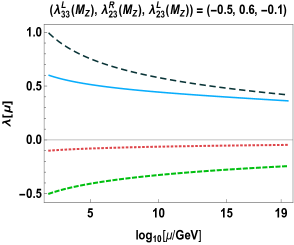
((d))    (d)

((e))    (e)

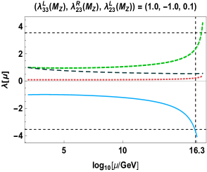
((f))    (f)

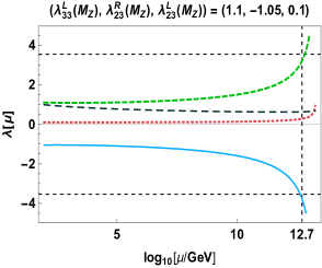
((g))    (g)

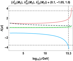
((h))    (h)

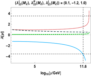
((i))    (i)

Figure 8: Behaviour of Yukawa couplings with various benchmark values at the EW scale. The labels of the couplings are given in the first plot. The dashed horizontal lines denote the values of the assumed perturbativity bound, $\pm\sqrt{4\pi}$. The dashed vertical line denotes the energy scale at which this bound is first reached.

IV.7 RG running of the Yukawa couplings and perturbativity

One of the questions raised by the introduction of new Yukawa couplings is whether the new model remains perturbative up to high-enough energies. This is particularly important in the GUT framework since the RG running of the gauge couplings is performed under the assumption of perturbativity. Fortunately, with the latest LHC data, we have quite a large available parameter space in the deep perturbative region, as can be seen in Fig. 7. While this suggests that the model is safe in terms of perturbativity as long as the new Yukawa couplings are small enough at the electroweak scale, it is still informative to investigate the RG running in detail, especially the case in which the Yukawa couplings take larger initial values. We address this issue in this part of the paper.

The equations for the RG running of the Yukawa couplings are given in Appendix A. Results for various benchmark cases are displayed in Fig. 8. Among the $S_{1}$ mass values we have considered in this paper, the most constrained parameter space is that of $M_{S_{1}}=2$ TeV. Therefore, we choose our benchmark values from the parameter space for this mass value, displayed in Fig. 7. Note that $\lambda^{L}_{33}(M_{Z})$ and $\lambda^{L}_{23}(M_{Z})$ cannot both be large and that $\lambda^{L}_{33}(M_{Z})$ and $\lambda^{R}_{23}(M_{Z})$ must have opposite signs, as can be seen in Fig. 7. When $\lambda^{L}_{23}(M_{Z})$ is taken in the interval $[-0.2,0.1]$, the system remains perturbative up to the grand unification scale, $\sim 10^{15}$-$10^{17}$ GeV, even when $|\lambda^{L}_{33}(M_{Z})|$, $|\lambda^{R}_{23}(M_{Z})|\approx 1$, as displayed in the first six plots in Fig. 8. However, it deteriorates quickly for larger values of $|\lambda^{L}_{33}(M_{Z})|$ and $|\lambda^{R}_{23}(M_{Z})|$ [Fig. 8(g)]. When $|\lambda^{L}_{23}(M_{Z})|$ is large, the parameter space is quite limited for $|\lambda^{L}_{33}(M_{Z})|$, which is in the $[0.10,0.15]$ band (Fig. 7). In this case as well, the system is well behaved up to $|\lambda^{L}_{23}(M_{Z})|$, $|\lambda^{R}_{23}(M_{Z})|\approx 1$ [e.g. Fig. 8(h)], and the situation declines for the values above in that the perturbativity bound is reached below the unification scale [e.g. Fig. 8(i)].

Note that although we perform the Yukawa RG running based on the SM augmented with a TeV scale leptoquark $S_{1}$ all the way up the UV, these equations are prone to changes above the intermediate symmetry-breaking scale provided that there is one (as in the examples studied in Sec. III), mainly due to contributions from the running of the scalars whose masses are around the intermediate scale. However, these effects are expected to be minor due to the corresponding beta-function coefficients not being large enough to significantly change the logarithmic RG running Altarelli:2013aqa . This is even more likely to be the case especially if this symmetry-breaking scale, for instance the scale in our scenario where the Pati-Salam symmetry is spontaneously broken to the symmetry of the SM, is considerably close to the scale of the $\mathrm{SO}(10)$ symmetry-breaking scale (as in the second case in Sec. III, namely model $A_{2}$), suggesting that the supposed modification in the Yukawa running is indeed not an issue of concern since the slow logarithmic running would most likely does not significantly alter the outcome in this small interval. Threshold corrections due to the intermediate scale are also known to be subleading to the one-loop running Babu:2016bmy .

Furthermore, although we have studied some specific examples for gauge coupling unification, there are no restrictions on the choice of the mass values of the high-energy field content regarding which fields remain heavy at the unification scale and which ones slide through the intermediate scale, as long as the gauge coupling unification is realized (and as long as the intermediate scale is high enough to evade the proton-decay constraints for the terms not forbidden by any symmetry in the Lagrangian). The main point of our case that we emphasize is that if an $\mathrm{SO}(10)$ theory is indeed the UV completion of the SM, then one may naturally anticipate a TeV scale leptoquark accompanying the SM Higgs field, and this could define the field content up to very high energies. Beyond that, one has the freedom to choose the high-energy particle content and the corresponding potential terms in the Lagrangian that lead to an appropriate symmetry-breaking sequence in which the Yukawa couplings remain in the perturbative realm above the intermediate symmetry-breaking scale. With this in mind, even the other cases, displayed in Fig. 8(g) and Fig. 8(i), that suffer from perturbativity problem at relatively low energies could arguably get a pass, as long as the high energy content of the theory is chosen such that the intermediate symmetry-breaking occurs before the perturbativity bound is reached and such that the couplings remain in the perturbative realm up to the unification scale.

We comment in passing on the unification-scale implications of our model regarding the fermion mass spectrum. It has been known in the literature that obtaining a realistic Yukawa sector in the $\mathrm{SO}(10)$ framework is not trivial. None of the single- and dual-field combinations of the scalar fields $\mathbf{10}_{H}$, $\mathbf{120}_{H}$, and $\mathbf{126}_{H}$ yields GUT-scale relations between fermion masses consistent with the SM values Bajc:2005zf ; Babu:2016bmy . On the other hand, it was concluded in Ref. Babu:2016bmy that a Higgs sector consisting of a real $\mathbf{10}_{H}$, a real $\mathbf{120}_{H}$, and a complex $\mathbf{126}_{H}$ can provide a fermion mass spectrum at the unification scale that matches the expected values obtained by the RG running of the SM with small threshold corrections at the intermediate scale. Since this is the scalar sector we adopt in this paper, it is informative to inspect whether the light leptoquark $S_{1}$ can register significant changes to the expected fermion mass values at the unification scale obtained via the SM RG running.

The results, obtained by using the equations given in Appendix A and the same values for the input parameters at $M_{Z}$ as in Ref. Babu:2016bmy , are given in Table 5, some of which are displayed in terms of mass ratios relevant in the $\mathrm{SO}(10)$ framework. The unification scale is selected as $M_{U}=2\times 10^{16}$ GeV, which is around the exponential midpoint of the unification scales of our models $A_{1}$ and $A_{2}$ discussed in Sec. III; small numerical differences depending on the $M_{U}$ value in that range is not relevant to our discussion here. Our values for the fermion masses at $M_{U}$ in the SM case differ from the ones in Ref. Babu:2016bmy by $1$-$5~{}\%$, which might be due to a combination of effects coming from the running of the right-handed neutrinos above the intermediate scale and the threshold corrections, both of which are ignored in our estimation. The results for the leptoquark case are given for three benchmark points in the $(\lambda_{33}^{L},\lambda_{23}^{R},\lambda_{23}^{L})$ parameter space that are consistent with the perturbativity analysis above. As expected, when all three of the new Yukawa couplings are in the deep perturbative region, the differences from the SM values remain insignificant. When the couplings get larger close to unity, some deviations are observed yet they do not become substantial. Therefore, we conclude that the addition of $S_{1}$ to the particle content up to the TeV scale does not lead to significant changes regarding the expected fermion masses at the unification scale and therefore the analysis of Ref. Babu:2016bmy , based on using the extrapolated SM values at the unification scale as input data in order to numerically fit them to the parameters of the Yukawa sector of their $\mathrm{SO}(10)$ model, can be applied in our case as well.

Table 5: Fermion masses at the unification scale $M_{U}=2\times 10^{16}$ GeV that are selected for the sake of argument as the exponential midpoint of the unification scales of the high-energy scenarios discussed in Sec. III. Clearly, inclusion of $S_{1}$ in the low-energy particle spectrum does not lead to significant changes in the fermion mass values at the unification scale compared to the SM predictions, especially in the deep perturbative region in the $(\lambda_{33}^{L},\lambda_{23}^{R},\lambda_{23}^{L})$ parameter space.

	$\;(0,0,0);\;\textrm{SM}\;\;\;$	$(0.5,-0.4,0.1)$	$(0.8,-0.9,0.1)$	$(0.1,-1.0,1.0)$
$m_{t}/m_{b}$	$75.57$	$75.66$	$76.37$	$75.36$
$m_{\tau}/m_{b}$	$1.63$	$1.74$	$2.31$	$4.28$
$m_{\mu}/m_{s}$	$4.41$	$4.46$	$4.46$	$3.94$
$m_{e}/m_{d}$	$0.400$	$0.401$	$0.401$	$0.401$
$m_{t}/{\footnotesize\textrm{GeV}}$	$79.32$	$79.52$	$83.46$	$78.14$
$m_{c}/{\footnotesize\textrm{GeV}}$	$0.254$	$0.254$	$0.275$	$0.344$
$m_{\mu}/(10^{-3}{\footnotesize\textrm{GeV}})$	$100.505$	$100.576$	$101.518$	$100.175$
$m_{e}/(10^{-3}{\footnotesize\textrm{GeV}})$	$0.476$	$0.476$	$0.481$	$0.475$
$m_{u}/(10^{-3}{\footnotesize\textrm{GeV}})$	$0.469$	$0.464$	$0.469$	$0.462$

V Summary and Discussions

In this paper, we considered the scenario that there is a single scalar leptoquark, $S_{1}$, at the TeV scale, and it is the colour-triplet component of a real $\mathbf{10}$ of $\mathrm{SO}(10)$, which also contains a $\mathrm{SU}(2)$ doublet which is identified as the SM Higgs. In this scenario, the leptoquark being the only scalar entity other than the SM Higgs is natural; a peculiar mass splitting between the components of $\mathbf{10}$ does not occur and the leptoquark picks up an electroweak-scale mass together with the SM Higgs, as expected. This is appealing because this leptoquark by itself can potentially explain the $B$-decay anomalies at the LHC Bauer:2015knc ; Becirevic:2016oho ; Cai:2017wry ; Freytsis:2015qca .

The $\mathrm{SO}(10)$ grand unification framework is an appealing scenario, which has been heavily studied in the literature Fritzsch:1974nn ; Chang:1983fu ; Chang:1984uy ; Chang:1984qr ; Deshpande:1992au ; Bajc:2005zf ; Bertolini:2009qj ; Babu:2012vc ; Altarelli:2013aqa ; Aydemir:2015oob ; Aydemir:2016qqj ; Babu:2015bna ; Babu:2016bmy . It unifies the three forces in the SM, explains the quantization of electric charge, provides numerous dark matter candidates, accommodates seesaw mechanism for small neutrino masses, and justifies the remarkable cancellation of anomalies through the anomaly-free nature of the $\mathrm{SO}(10)$ gauge group. Moreover, the fermionic content of the SM fits elegantly in $\mathbf{16}_{F}$, including a right-handed neutrino for each family. The particles in the SM (except probably the neutrinos) acquire masses up to the electroweak scale through interacting with the electroweak-scale Higgs field, which is generally assigned to a real $\mathbf{10}_{H}$. Considering that the leptoquark $S_{1}$ is the only other component in $\mathbf{10}_{H}$, a TeV scale $S_{1}$, from this perspective, is consistent with the idea that it is the last piece of the puzzle regarding the particle content up to the electroweak scale (modulo the right-handed neutrinos). Therefore, the possible detection of $S_{1}$, in the absence of any other new particles, at the TeV scale could be interpreted as evidence in favour of $\mathrm{SO}(10)$ grand unification.

One obvious issue of concern is proton decay since the leptoquark $S_{1}$ possesses the right quantum numbers for it to couple to potentially dangerous diquark operators. On the other hand, the proton stability could possibly be ensured through various mechanisms Cox:2016epl ; Bajc:2005zf ; Pati:1974yy ; Bauer:2015knc ; Dvali:1995hp ; Aydemir:2018cbb . In this paper, we ensured the proton stability by assuming a discrete symmetry that is imposed in an ad hoc manner below the Pati-Salam breaking scale. It would certainly be more compelling to realize a similar mechanism at the fundamental level although it seems unlikely that it would interfere with the bottom line of this work.

Having a single $S_{1}$ leptoquark at the TeV scale as the only new physics remnant from our $\mathrm{SO}(10)$ GUT model, we investigated how competent this $S_{1}$ is at addressing the $R_{D^{(*)}}$ anomalies while simultaneously satisfying other relevant constraints from flavour, electroweak and the direct LHC searches. We adopted a specific Yukawa coupling texture with only three free (real) nonzero couplings viz. $\lambda_{23}^{L}$, $\lambda_{33}^{L}$ and $\lambda_{23}^{R}$. We have found that this minimal consideration can alleviate the potential tension between the $R_{D^{(*)}}$-favoured region and the $R_{K^{(*)}}^{\nu\nu}$ measurements. The $Z\to\tau\tau$ decay constrains $\lambda_{33}^{L}$ whereas the $\tau\tau$ resonance search at the LHC puts complimentary bounds on $\lambda_{23}^{L}$ and $\lambda_{23}^{R}$. By combining these constraints with all the relevant flavour constraints coming from the latest data on $R_{D^{(*)}}$, $F_{L}{(D^{*})}$, $P_{\tau}(D^{*})$, $R_{K^{(*)}}^{\nu\nu}$ we have found that a substantial region of the $R_{D^{(*)}}$-favoured parameter space is allowed. Our multiparameter analysis clearly shows that contrary to the common perception, a single leptoquark solution to the observed $R_{D^{(*)}}$ anomalies with $S_{1}$ is still a viable solution.

Evidently, by introducing new degrees of freedom into our framework, one can, a priori, enlarge the allowed parameter region. For example, by considering some of the couplings as complex or by choosing a complex (instead of a real) $\mathbf{10}$ representation of $\mathrm{SO}(10)$, which will introduce an additional $S_{1}$ and another complex scalar doublet at the TeV scale, one can relax our obtained bounds. We also pointed out search strategies for $S_{1}$ at the LHC using symmetric and asymmetric pair- and single-production channels. Systematic studies of these channels are discussed elsewhere Chandak:2019iwj .

Appendix A Renormalization group running of the Yukawa couplings

The new Yukawa matrices in the Lagrangian given in Eq. (12) are taken in our setup as

$$\Lambda^{L}\rightarrow\left(\begin{array}[]{ccc}0&0&0\\ 0&0&\lambda^{L}_{23}\\ 0&0&\lambda^{L}_{33}\end{array}\right)~{}\mbox{and}~{}\Lambda^{R}\rightarrow\left(\begin{array}[]{ccc}0&0&0\\ 0&0&\lambda^{R}_{23}\\ 0&0&0\end{array}\right).\qquad$$ (54)

Following Ref. Machacek:1983fi (or implementing the model in SARAH Staub:2012pb ), the corresponding one-loop RG equations can be found as

$$16\pi^{2}\beta_{\lambda^{R}_{23}} = 3\left(\lambda^{R}_{23}\right)^{3}-\lambda^{R}_{23}\left(\frac{13}{3}g_{1}^{2}+4g_{3}^{2}\right)$$ (56)

$$+2\lambda^{R}_{23}\left(\left(\lambda^{L}_{23}\right)^{2}+\left(\lambda^{L}_{33}\right)^{2}\right),$$

$$16\pi^{2}\beta_{\lambda^{L}_{33}} = 4\left(\lambda^{L}_{33}\right)^{3}-\lambda^{L}_{33}\Big{(}-\frac{y_{t}^{2}}{2}+\frac{5}{6}g_{1}^{2}+\frac{9}{2}g_{2}^{2}$$ (57)

$$+4g_{3}^{2}\Big{)}+\lambda^{L}_{33}\left(\left(\lambda^{R}_{23}\right)^{2}+4\left(\lambda^{L}_{23}\right)^{2}\right),$$

$$16\pi^{2}\beta_{\lambda^{L}_{23}} = 4\left(\lambda^{L}_{23}\right)^{3}-\lambda^{L}_{23}\left(\frac{5}{6}g_{1}^{2}+\frac{9}{2}g_{2}^{2}+4g_{3}^{2}\right)$$ (58)

$$+\lambda^{L}_{23}\left(\left(\lambda^{R}_{23}\right)^{2}+4\left(\lambda^{L}_{33}\right)^{2}\right),$$

$$16\pi^{2}\beta_{y_{t}} = 3y_{t}^{3}+y_{t}\left(\frac{3}{2}y_{t}^{3}-\frac{17}{12}g_{1}^{2}-\frac{9}{4}g_{2}^{2}-8g_{3}^{2}\right)$$ (59)

$$+\frac{1}{2}y_{t}\left(\lambda^{L}_{33}\right)^{2},$$

$$16\pi^{2}\beta_{y_{c}} = y_{c}\left(3y_{t}^{2}-\frac{17}{12}g_{1}^{2}-\frac{9}{4}g_{2}^{2}-8g_{3}^{2}\right)$$ (60)

$$+\frac{1}{2}y_{c}\left(\left(\lambda^{R}_{23}\right)^{2}+\left(\lambda^{L}_{23}\right)^{2}\right),$$

$$16\pi^{2}\beta_{y_{u}} = y_{u}\left(3y_{t}^{2}-\frac{17}{12}g_{1}^{2}-\frac{9}{4}g_{2}^{2}-8g_{3}^{2}\right),$$ (61)

$$16\pi^{2}\beta_{y_{b}} = y_{b}\left(\frac{3}{2}y_{t}^{2}-\frac{5}{12}g_{1}^{2}-\frac{9}{4}g_{2}^{2}-8g_{3}^{2}\right)$$ (62)

$$+\frac{1}{2}y_{b}\left(\lambda^{L}_{33}\right)^{2},$$

$$16\pi^{2}\beta_{y_{s}} = y_{s}\left(3y_{t}^{2}-\frac{5}{12}g_{1}^{2}-\frac{9}{4}g_{2}^{2}-8g_{3}^{2}\right)$$ (63)

$$+\frac{1}{2}y_{s}\left(\lambda^{L}_{23}\right)^{2},$$

$$16\pi^{2}\beta_{y_{d}} = y_{d}\left(3y_{t}^{2}-\frac{5}{12}g_{1}^{2}-\frac{9}{4}g_{2}^{2}-8g_{3}^{2}\right),$$ (64)

$$16\pi^{2}\beta_{y_{e}} = y_{e}\left(3y_{t}^{2}-\frac{15}{4}g_{1}^{2}-\frac{9}{4}g_{2}^{2}\right),$$ (65)

$$16\pi^{2}\beta_{y_{\mu}} = y_{\mu}\left(3y_{t}^{2}-\frac{15}{4}g_{1}^{2}-\frac{9}{4}g_{2}^{2}\right),$$ (66)

$$16\pi^{2}\beta_{y_{\tau}} = y_{\tau}\left(3y_{t}^{2}-\frac{15}{4}g_{1}^{2}-\frac{9}{4}g_{2}^{2}\right)$$ (67)

$$+\frac{3}{2}y_{\tau}\left(\left(\lambda^{R}_{23}\right)^{2}+\left(\lambda^{L}_{23}\right)^{2}+\left(\lambda^{L}_{33}\right)^{2}\right),\qquad$$

where $\beta_{y}\equiv\mu\dfrac{dy}{d\mu}$ and the RG running of the gauge couplings are performed in the usual way according to Eq. (13). In the Yukawa running above, only the dominant terms are taken into account since the subleading ones are significantly suppressed and have no noticeable effects on our analysis.

References

- (1) BaBar collaboration, J. P. Lees et al., Evidence for an excess of decays, Phys. Rev. Lett. 109 (2012) 101802, [1205.5442].
- (2) BaBar collaboration, J. P. Lees et al., Measurement of an Excess of Decays and Implications for Charged Higgs Bosons, Phys. Rev. D88 (2013) 072012, [1303.0571].
- (3) LHCb collaboration, R. Aaij et al., Test of lepton universality using decays, Phys. Rev. Lett. 113 (2014) 151601, [1406.6482].
- (4) LHCb collaboration, R. Aaij et al., Test of lepton universality with decays, JHEP 08 (2017) 055, [1705.05802].
- (5) LHCb collaboration, R. Aaij et al., Measurement of the ratio of branching fractions , Phys. Rev. Lett. 115 (2015) 111803, [1506.08614]. [Erratum: Phys. Rev. Lett.115,no.15,159901(2015)].
- (6) LHCb collaboration, R. Aaij et al., Measurement of the ratio of the and branching fractions using three-prong -lepton decays, Phys. Rev. Lett. 120 (2018) 171802, [1708.08856].
- (7) LHCb collaboration, R. Aaij et al., Test of Lepton Flavor Universality by the measurement of the branching fraction using three-prong decays, Phys. Rev. D97 (2018) 072013, [1711.02505].
- (8) Belle collaboration, M. Huschle et al., Measurement of the branching ratio of relative to decays with hadronic tagging at Belle, Phys. Rev. D92 (2015) 072014, [1507.03233].
- (9) Belle collaboration, Y. Sato et al., Measurement of the branching ratio of relative to decays with a semileptonic tagging method, Phys. Rev. D94 (2016) 072007, [1607.07923].
- (10) Belle collaboration, S. Hirose et al., Measurement of the lepton polarization and in the decay , Phys. Rev. Lett. 118 (2017) 211801, [1612.00529].
- (11) Belle collaboration, S. Hirose et al., Measurement of the lepton polarization and in the decay with one-prong hadronic decays at Belle, Phys. Rev. D97 (2018) 012004, [1709.00129].
- (12) D. Bigi and P. Gambino, Revisiting , Phys. Rev. D94 (2016) 094008, [1606.08030].
- (13) F. U. Bernlochner, Z. Ligeti, M. Papucci and D. J. Robinson, Combined analysis of semileptonic decays to and : , , and new physics, Phys. Rev. D95 (2017) 115008, [1703.05330]. [erratum: Phys. Rev. D97 (2018) 059902].
- (14) D. Bigi, P. Gambino and S. Schacht, , , and the Heavy Quark Symmetry relations between form factors, JHEP 11 (2017) 061, [1707.09509].
- (15) S. Jaiswal, S. Nandi and S. K. Patra, Extraction of from and the Standard Model predictions of , JHEP 12 (2017) 060, [1707.09977].
- (16) HFLAV collaboration, Y. Amhis et al., Averages of -hadron, -hadron, and -lepton properties as of summer 2016, Eur. Phys. J. C77 (2017) 895, [1612.07233]. We have used the spring 2019 averages from https://hflav-eos.web.cern.ch/hflav-eos/semi/spring19/html/RDsDsstar/RDRDs.html.
- (17) G. Hiller and F. Kruger, More model-independent analysis of processes, Phys. Rev. D69 (2004) 074020, [hep-ph/0310219].
- (18) M. Bordone, G. Isidori and A. Pattori, On the Standard Model predictions for and , Eur. Phys. J. C76 (2016) 440, [1605.07633].
- (19) I. Dors̆ner, S. Fajfer, N. Kos̆nik and I. Nis̆andz̆ić, Minimally flavored colored scalar in and the mass matrices constraints, JHEP 11 (2013) 084, [1306.6493].
- (20) Y. Sakaki, M. Tanaka, A. Tayduganov and R. Watanabe, Testing leptoquark models in , Phys. Rev. D88 (2013) 094012, [1309.0301].
- (21) M. Freytsis, Z. Ligeti and J. T. Ruderman, Flavor models for , Phys. Rev. D92 (2015) 054018, [1506.08896].
- (22) M. Bauer and M. Neubert, Minimal Leptoquark Explanation for the , , and Anomalies, Phys. Rev. Lett. 116 (2016) 141802, [1511.01900].
- (23) B. Dumont, K. Nishiwaki and R. Watanabe, LHC constraints and prospects for scalar leptoquark explaining the anomaly, Phys. Rev. D94 (2016) 034001, [1603.05248].
- (24) D. Das, C. Hati, G. Kumar and N. Mahajan, Towards a unified explanation of , and anomalies in a left-right model with leptoquarks, Phys. Rev. D94 (2016) 055034, [1605.06313].
- (25) D. Bečirević, N. Košnik, O. Sumensari and R. Zukanovich Funchal, Palatable Leptoquark Scenarios for Lepton Flavor Violation in Exclusive modes, JHEP 11 (2016) 035, [1608.07583].
- (26) D. Bečirević, S. Fajfer, N. Košnik and O. Sumensari, Leptoquark model to explain the -physics anomalies, and , Phys. Rev. D94 (2016) 115021, [1608.08501].
- (27) D. A. Faroughy, A. Greljo and J. F. Kamenik, Confronting lepton flavor universality violation in B decays with high- tau lepton searches at LHC, Phys. Lett. B764 (2017) 126–134, [1609.07138].
- (28) G. Hiller, D. Loose and K. Schönwald, Leptoquark Flavor Patterns & Decay Anomalies, JHEP 12 (2016) 027, [1609.08895].
- (29) C.-H. Chen, T. Nomura and H. Okada, Excesses of muon , , and in a leptoquark model, Phys. Lett. B774 (2017) 456–464, [1703.03251].
- (30) A. Crivellin, D. Müller and T. Ota, Simultaneous explanation of R(D(∗)) and : the last scalar leptoquarks standing, JHEP 09 (2017) 040, [1703.09226].
- (31) D. Bečirević and O. Sumensari, A leptoquark model to accommodate and , JHEP 08 (2017) 104, [1704.05835].
- (32) Y. Cai, J. Gargalionis, M. A. Schmidt and R. R. Volkas, Reconsidering the One Leptoquark solution: flavor anomalies and neutrino mass, JHEP 10 (2017) 047, [1704.05849].
- (33) W. Altmannshofer, P. Bhupal Dev and A. Soni, anomaly: A possible hint for natural supersymmetry with -parity violation, Phys. Rev. D96 (2017) 095010, [1704.06659].
- (34) N. Assad, B. Fornal and B. Grinstein, Baryon Number and Lepton Universality Violation in Leptoquark and Diquark Models, Phys. Lett. B777 (2018) 324–331, [1708.06350].
- (35) M. Jung and D. M. Straub, Constraining new physics in transitions, JHEP 01 (2019) 009, [1801.01112].
- (36) A. Biswas, D. K. Ghosh, S. K. Patra and A. Shaw, anomalies in light of extended scalar sectors, 1801.03375.
- (37) P. Bandyopadhyay and R. Mandal, Revisiting scalar leptoquark at the LHC, Eur. Phys. J. C78 (2018) 491, [1801.04253].
- (38) U. Aydemir, D. Minic, C. Sun and T. Takeuchi, -decay anomalies and scalar leptoquarks in unified Pati-Salam models from noncommutative geometry, JHEP 09 (2018) 117, [1804.05844].
- (39) D. Marzocca, Addressing the B-physics anomalies in a fundamental Composite Higgs Model, JHEP 07 (2018) 121, [1803.10972].
- (40) D. Bečirević, I. Doršner, S. Fajfer, N. Košnik, D. A. Faroughy and O. Sumensari, Scalar leptoquarks from grand unified theories to accommodate the -physics anomalies, Phys. Rev. D98 (2018) 055003, [1806.05689].
- (41) J. Kumar, D. London and R. Watanabe, Combined Explanations of the and Anomalies: a General Model Analysis, Phys. Rev. D99 (2019) 015007, [1806.07403].
- (42) Q.-Y. Hu, X.-Q. Li, Y. Muramatsu and Y.-D. Yang, R-parity violating solutions to the anomaly and their GUT-scale unifications, Phys. Rev. D99 (2019) 015008, [1808.01419].
- (43) T. Faber, M. Hudec, M. Malinský, P. Meinzinger, W. Porod and F. Staub, A unified leptoquark model confronted with lepton non-universality in -meson decays, Phys. Lett. B787 (2018) 159–166, [1808.05511].
- (44) J. Heeck and D. Teresi, Pati-Salam explanations of the B-meson anomalies, JHEP 12 (2018) 103, [1808.07492].
- (45) A. Angelescu, D. Bečirević, D. A. Faroughy and O. Sumensari, Closing the window on single leptoquark solutions to the -physics anomalies, JHEP 10 (2018) 183, [1808.08179].
- (46) S. Bifani, S. Descotes-Genon, A. Romero Vidal and M.-H. Schune, Review of Lepton Universality tests in decays, J. Phys. G46 (2019) 023001, [1809.06229].
- (47) S. Bansal, R. M. Capdevilla and C. Kolda, Constraining the minimal flavor violating leptoquark explanation of the anomaly, Phys. Rev. D99 (2019) 035047, [1810.11588].
- (48) T. Mandal, S. Mitra and S. Raz, motivated leptoquark scenarios: Impact of interference on the exclusion limits from LHC data, Phys. Rev. D99 (2019) 055028, [1811.03561].
- (49) S. Iguro, T. Kitahara, R. Watanabe and K. Yamamoto, polarization vs. anomalies in the leptoquark models, 1811.08899.
- (50) J. Aebischer, A. Crivellin and C. Greub, QCD Improved Matching for Semi-Leptonic Decays with Leptoquarks, 1811.08907.
- (51) S. Bar-Shalom, J. Cohen, A. Soni and J. Wudka, Phenomenology of TeV-scale scalar Leptoquarks in the EFT, 1812.03178.
- (52) T. J. Kim, P. Ko, J. Li, J. Park and P. Wu, Correlation between and top quark FCNC decays in leptoquark models, 1812.08484.
- (53) P. Arnan, D. Bečirević, F. Mescia and O. Sumensari, Probing low energy scalar leptoquarks by the leptonic and couplings, JHEP 02 (2019) 109, [1901.06315].
- (54) B. Bhattacharya, A. Datta, J.-P. Guévin, D. London and R. Watanabe, Simultaneous Explanation of the and Puzzles: a Model Analysis, JHEP 01 (2017) 015, [1609.09078].
- (55) S. Sahoo and R. Mohanta, Impact of vector leptoquark on anomalies, J. Phys. G45 (2018) 085003, [1806.01048].
- (56) A. Crivellin, C. Greub, D. Muller and F. Saturnino, Importance of Loop Effects in Explaining the Accumulated Evidence for New Physics in B Decays with a Vector Leptoquark, Phys. Rev. Lett. 122 (2019) 011805, [1807.02068].
- (57) A. Biswas, D. Kumar Ghosh, N. Ghosh, A. Shaw and A. K. Swain, Novel collider signature of Leptoquark and observables, 1808.04169.
- (58) S. Balaji, R. Foot and M. A. Schmidt, A chiral SU(4) explanation of the anomalies, Phys. Rev. D99 (2019) 015029, [1809.07562].
- (59) A. Biswas, A. K. Swain and A. Shaw, Collider signature of Leptoquark with flavour observables, 1811.08887.
- (60) J. Roy, Probing leptoquark chirality via top polarization at the Colliders, 1811.12058.
- (61) B. Fornal, S. A. Gadam and B. Grinstein, Left-Right SU(4) Vector Leptoquark Model for Flavor Anomalies, 1812.01603.
- (62) H. Fritzsch and P. Minkowski, Unified Interactions of Leptons and Hadrons, Annals Phys. 93 (1975) 193–266.
- (63) H. Georgi, The State of the Art–Gauge Theories, AIP Conf. Proc. 23 (1975) 575–582.
- (64) D. Chang, R. N. Mohapatra and M. K. Parida, Decoupling Parity and SU(2)-R Breaking Scales: A New Approach to Left-Right Symmetric Models, Phys. Rev. Lett. 52 (1984) 1072.
- (65) D. Chang, R. N. Mohapatra and M. K. Parida, A New Approach to Left-Right Symmetry Breaking in Unified Gauge Theories, Phys. Rev. D30 (1984) 1052.
- (66) D. Chang, R. N. Mohapatra, J. Gipson, R. E. Marshak and M. K. Parida, Experimental Tests of New SO(10) Grand Unification, Phys. Rev. D31 (1985) 1718.
- (67) N. G. Deshpande, E. Keith and P. B. Pal, Implications of LEP results for SO(10) grand unification, Phys. Rev. D46 (1993) 2261–2264.
- (68) B. Bajc, A. Melfo, G. Senjanovic and F. Vissani, Yukawa sector in non-supersymmetric renormalizable SO(10), Phys. Rev. D73 (2006) 055001, [hep-ph/0510139].
- (69) S. Bertolini, L. Di Luzio and M. Malinsky, Intermediate mass scales in the non-supersymmetric SO(10) grand unification: A Reappraisal, Phys. Rev. D80 (2009) 015013, [0903.4049].
- (70) K. S. Babu and R. N. Mohapatra, Coupling Unification, GUT-Scale Baryogenesis and Neutron-Antineutron Oscillation in SO(10), Phys. Lett. B715 (2012) 328–334, [1206.5701].
- (71) G. Altarelli and D. Meloni, A non supersymmetric SO(10) grand unified model for all the physics below , JHEP 08 (2013) 021, [1305.1001].
- (72) U. Aydemir, SO(10) grand unification in light of recent LHC searches and colored scalars at the TeV-scale, Int. J. Mod. Phys. A31 (2016) 1650034, [1512.00568].
- (73) U. Aydemir and T. Mandal, LHC probes of TeV-scale scalars in grand unification, Adv. High Energy Phys. 2017 (2017) 7498795, [1601.06761].
- (74) K. S. Babu and S. Khan, Minimal nonsupersymmetric model: Gauge coupling unification, proton decay, and fermion masses, Phys. Rev. D92 (2015) 075018, [1507.06712].
- (75) K. S. Babu, B. Bajc and S. Saad, Yukawa Sector of Minimal SO(10) Unification, JHEP 02 (2017) 136, [1612.04329].
- (76) P. Cox, A. Kusenko, O. Sumensari and T. T. Yanagida, SU(5) Unification with TeV-scale Leptoquarks, JHEP 03 (2017) 035, [1612.03923].
- (77) J. C. Pati and A. Salam, Lepton Number as the Fourth Color, Phys. Rev. D10 (1974) 275–289. [Erratum: Phys. Rev.D11,703(1975)].
- (78) G. R. Dvali, Light color triplet Higgs is compatible with proton stability: An Alternative approach to the doublet - triplet splitting problem, Phys. Lett. B372 (1996) 113–120, [hep-ph/9511237].
- (79) A. Maiezza, M. Nemevsek, F. Nesti and G. Senjanovic, Left-Right Symmetry at LHC, Phys. Rev. D82 (2010) 055022, [1005.5160].
- (80) P. Bandyopadhyay and R. Mandal, Vacuum stability in an extended standard model with a leptoquark, Phys. Rev. D95 (2017) 035007, [1609.03561].
- (81) D. R. T. Jones, The Two Loop beta Function for a Gauge Theory, Phys. Rev. D25 (1982) 581.
- (82) M. Lindner and M. Weiser, Gauge coupling unification in left-right symmetric models, Phys. Lett. B383 (1996) 405–414, [hep-ph/9605353].
- (83) Particle Data Group collaboration, C. Patrignani et al., Review of Particle Physics, Chin. Phys. C40 (2016) 100001.
- (84) SLD Electroweak Group, DELPHI, ALEPH, SLD, SLD Heavy Flavour Group, OPAL, LEP Electroweak Working Group, L3 collaboration, S. Schael et al., Precision electroweak measurements on the resonance, Phys. Rept. 427 (2006) 257–454, [hep-ex/0509008].
- (85) Super-Kamiokande collaboration, K. Abe et al., Search for proton decay via and in 0.31 megaton 7 years exposure of the Super-Kamiokande water Cherenkov detector, Phys. Rev. D95 (2017) 012004, [1610.03597].
- (86) P. Langacker, Grand Unified Theories and Proton Decay, Phys. Rept. 72 (1981) 185.
- (87) CMS collaboration, A. M. Sirunyan et al., Search for third-generation scalar leptoquarks decaying to a top quark and a lepton at 13 TeV, Eur. Phys. J. C78 (2018) 707, [1803.02864].
- (88) CMS collaboration, A. M. Sirunyan et al., Constraints on models of scalar and vector leptoquarks decaying to a quark and a neutrino at 13 TeV, Phys. Rev. D98 (2018) 032005, [1805.10228].
- (89) S. Bhattacharya, S. Nandi and S. Kumar Patra, Decays: a catalogue to compare, constrain, and correlate new physics effects, Eur. Phys. J. C79 (2019) 268, [1805.08222].
- (90) Belle, Belle-II collaboration, K. Adamczyk, Semitauonic decays at Belle/Belle II, in 10th International Workshop on the CKM Unitarity Triangle (CKM 2018) Heidelberg, Germany, September 17-21, 2018, 2019. 1901.06380.
- (91) M. Tanaka and R. Watanabe, New physics in the weak interaction of , Phys. Rev. D87 (2013) 034028, [1212.1878].
- (92) M. Blanke, A. Crivellin, S. de Boer, T. Kitahara, M. Moscati, U. Nierste et al., Impact of polarization observables and on new physics explanations of the anomaly, Phys. Rev. D99 (2019) 075006, [1811.09603].
- (93) Belle collaboration, J. Grygier et al., Search for decays with semileptonic tagging at Belle, Phys. Rev. D96 (2017) 091101, [1702.03224]. [Addendum: Phys. Rev.D97,no.9,099902(2018)].
- (94) C. Degrande, C. Duhr, B. Fuks, D. Grellscheid, O. Mattelaer and T. Reiter, UFO - The Universal FeynRules Output, Comput. Phys. Commun. 183 (2012) 1201–1214, [1108.2040].
- (95) J. Alwall, R. Frederix, S. Frixione, V. Hirschi, F. Maltoni, O. Mattelaer et al., The automated computation of tree-level and next-to-leading order differential cross sections, and their matching to parton shower simulations, JHEP 07 (2014) 079, [1405.0301].
- (96) R. D. Ball et al., Parton distributions with LHC data, Nucl. Phys. B867 (2013) 244–289, [1207.1303].
- (97) T. Mandal, S. Mitra and S. Seth, Pair Production of Scalar Leptoquarks at the LHC to NLO Parton Shower Accuracy, Phys. Rev. D93 (2016) 035018, [1506.07369].
- (98) T. Mandal and S. Mitra, Probing Color Octet Electrons at the LHC, Phys. Rev. D87 (2013) 095008, [1211.6394].
- (99) T. Mandal, S. Mitra and S. Seth, Single Productions of Colored Particles at the LHC: An Example with Scalar Leptoquarks, JHEP 07 (2015) 028, [1503.04689].
- (100) T. Mandal, S. Mitra and S. Seth, Probing Compositeness with the CMS & Data, Phys. Lett. B758 (2016) 219–225, [1602.01273].
- (101) S. Bansal, R. M. Capdevilla, A. Delgado, C. Kolda, A. Martin and N. Raj, Hunting leptoquarks in monolepton searches, Phys. Rev. D98 (2018) 015037, [1806.02370].
- (102) ATLAS collaboration, M. Aaboud et al., Search for additional heavy neutral Higgs and gauge bosons in the ditau final state produced in 36 fb-1 of pp collisions at TeV with the ATLAS detector, JHEP 01 (2018) 055, [1709.07242].
- (103) ATLAS collaboration, M. Aaboud et al., Search for High-Mass Resonances Decaying to in pp Collisions at TeV with the ATLAS Detector, Phys. Rev. Lett. 120 (2018) 161802, [1801.06992].
- (104) K. Chandak, T. Mandal and S. Mitra, Hunting for scalar leptoquarks with boosted tops and light leptons, Phys. Rev. D100 (2019) 075019, [1907.11194].
- (105) M. E. Machacek and M. T. Vaughn, Two Loop Renormalization Group Equations in a General Quantum Field Theory. 2. Yukawa Couplings, Nucl. Phys. B236 (1984) 221–232.
- (106) F. Staub, SARAH 3.2: Dirac Gauginos, UFO output, and more, Comput. Phys. Commun. 184 (2013) 1792–1809, [1207.0906].