Fractional Conductance in Strongly Interacting 1D Systems

Abstract

We study one dimensional clean systems with few channels and strong electron-electron interactions. We find that in several circumstances, even when time reversal symmetry holds, they may lead to two terminal fractional quantized conductance and fractional shot noise. The condition on the commensurability of the Fermi momenta of the different channels and the strength of interactions resulting in such remarkable phenomena are explored using abelian bosonization. Finite temperature and length effects are accounted for by a generalization of the Luther-Emery re-fermionization at specific values of the interaction strength. We discuss the connection of our model to recent experiments in confined 2DEG, featuring possible fractional conductance plateaus. One of the most dominant observed fractions, with two terminal conductance equals to $\frac{2}{5}\frac{e^{2}}{h}$, is found in several scenarios of our model. Finally, we discuss how at very small energy scales the conductance returns to an integer value and the role of disorder.

Introduction and main results.— Fractional quantum Hall (FQH) effect, exhibiting a fractionally quantized value of the Hall conductance in units of $\frac{e^{2}}{h}$ Klitzing et al. (1980); Tsui et al. (1982), is a hallmark of strongly correlated electron systems, featuring composite particles, fractionally charged excitations, and fractional exchange statistics Laughlin (1983); Haldane (1983); Jain (1989). In recent years, theoretical studies of very clean one-dimensional (1D) quantum nano-wires with broken time reversal symmetry predict fractional values of the two-terminal conductance Oreg et al. (2014), as well as fractional shot noise Cornfeld et al. (2015). In contrast to the quantum Hall effect the one-dimensional wires are not topologically protected from the effect of impurity scattering, and hence observation of approximate fractional conductance and shot noise requires high degrees of purity.

Interest in such fractional states has risen recently, with experimental evidence for fractional transport in split-gate 1D constrictions made in germanium two-dimensional layers Gul et al. (2018), and in GaAs/AlGaAs heterostructures, even in the absence of an external magnetic field Kumar et al. (2018). Strong interactions between the quasi-particles in 1D are expected to play an important role in determining transport properties, especially when the electronic confinement in the transverse direction is somewhat relaxed Meyer and Matveev (2009); Welander et al. (2010).

In this manuscript, we explore a two-band fermionic 1D system, that bands for example could be, but not necessarily are, the spin degree of freedom. We find that even in the absence of time-reversal breaking the combination of tuning of the chemical potentials of the bands, and very strong inter-band interactions, leads to universal fractional transport properties at intermediate, and experimentally relevant, energy scales. We argue how in the very clean case at ultra-small temperatures, the conductance recovers an integer value. The role of disorder is discussed in the supplementary materials (SM) Sec. S.E.

We perform finite temperature and length analysis of the two-terminal conductance, employing RG analysis procedure and re-fermionization at specific values of the interaction that generalizes the Luther-Emery point Luther and Emery (1974). Finally, we use our novel results to suggest plausible scenarios that fit reported measurements, including conductance equals to $\frac{2}{5}$ in units of $\frac{e^{2}}{h}$; which is one of the most experimentally predominant fractions Kumar et al. (2018).

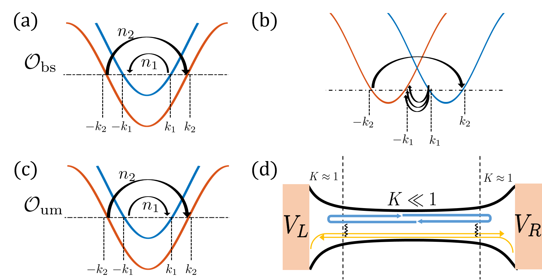
Figure 1: (a) Two-band dispersion with an example of a backscatering $\mathcal{O}_{{\rm bs}}$ process which conserves momentum when the chemical potential (horizontal dashed line) is such that $n_{1}k_{1}=n_{2}k_{2}$. (b) An example of a time-reversal invariant backscattering process, $\left(n_{1},n_{2}\right)=\left(3,1\right)$, occurring for fractional filling of a Rashba nano-wire, see SM Sec. S.C Sup . (c) Similarly to (a), an umklapp process $\mathcal{O}_{\mathrm{um}}$ with a net momentum change, conserves lattice momentum when $n_{1}k_{1}+n_{2}k_{2}=\pi\cdot\mathrm{integer}$, stabilizing a fractional Mott-insulator phase. (d) Illustration of a scenario where both bands interact throughout out the wire, yet one is confined and does not reach the reservoirs. This leads to a variety of possible fractional conductance values, see SM Sec. S.A Sup .

At the core of our analysis is the observation that when the electro-chemical potential $\mu$ is tuned properly, the backscattering momentum of $n_{1}$ right moving electrons at the Fermi level, is compensated by backward scattering of $n_{2}$ left moving electrons (and vice versa), so that multi-electron scattering processes occur in a clean momentum conserving system (see Fig. 1a). Such processes are relevant in the RG sense when interactions inside the wire are sufficiently strong. Remarkably, time-reversal symmetry is not necessarily broken when $\left|n_{1}+n_{2}\right|$ is even (see SM Sec. S.C). In the presence of a lattice umklapp processes may occur, they are formally accounted for by changing the relative sign of $n_{1},n_{2}$, see Fig. 1c.

Theoretical model.— We consider a 1D system which hosts two interacting electron species, with annihilation operators $c_{1}\left(x\right)$ and $c_{2}\left(x\right)$ at position $x$ and different chemical potentials $\mu_{i}$. The Hamiltonian is

$$H =\int dx\,c_{i}^{\dagger}\left(x\right)\left[\delta_{ij}\left(-\mu_{i}-\frac{\partial_{x}^{2}}{2m_{i}}\right)\right]c_{j}\left(x\right)$$

$$+\int dx\int dx^{\prime}\rho_{i}\left(x\right)U_{ij}\left(x,x^{\prime}\right)\rho_{j}\left(x^{\prime}\right),$$ (1)

where $\rho_{i}=c_{i}^{\dagger}c_{i}$, $U_{ij}$ is the interaction matrix, and summation over repeated indices, $i,j=1,2$, is implied. The model (1) is conveniently analyzed in the framework of abelian bosonization Giamarchi and Press (2004); Voit (1995). Linearizing the spectrum around the Fermi energy, the fermionic operators are decomposed into chiral modes, such that $c_{i}=\psi_{R}^{i}+\psi_{L}^{i}$, with $R$ ($L$) being the right (left) moving mode. These are then represented in terms of bosonic variables

$$\psi_{r}^{i}\sim\frac{1}{\sqrt{2\pi a}}e^{irk_{i}x}e^{-i\left(r\phi_{i}-\theta_{i}\right)},$$ (2)

with $k_{i}$ the Fermi momentum of species $i$, $a$ is a short-distance cutoff, $r=+1$ ($-1$) for right (left) movers, and the bosonic variables satisfy the algebra $\left[\phi_{i}\left(x\right),\partial_{x}\theta_{j}\left(x^{\prime}\right)\right]=i\pi\delta_{ij}\delta\left(x-x^{\prime}\right).$ The operator $-\frac{1}{\pi}\partial_{x}\phi_{i}$ ($\frac{1}{\pi}\partial_{t}\phi_{i}$) represents the normally-ordered charge (current) density of the $i$ species. The forward scattering part of the interaction $U$ is incorporated into the Hamiltonian $H_{{\rm fs}}$ by employing proper Luttinger parameters, and diagonalized by defining $\phi_{\pm}=\frac{1}{\sqrt{2}}\left(\phi_{1}\pm\phi_{2}\right)$ and $\theta_{\pm}=\frac{1}{\sqrt{2}}\left(\theta_{1}\pm\theta_{2}\right)$, such that

$$H_{{\rm fs}}=\sum_{\eta=\pm}\frac{u_{\eta}}{2\pi}\int dx\left[\frac{1}{K_{\eta}(x)}\left(\partial_{x}\phi_{\eta}\right)^{2}+K_{\eta}(x)\left(\partial_{x}\theta_{\eta}\right)^{2}\right].$$ (3)

Note that whereas the $\left(+\right)$ sector in (3) corresponds to the total charge sector, the $\left(-\right)$ does not necessarily represent spin. The distinction between different species is kept general at this point. The Luttinger parameters may be evaluated for weak interactions yielding: $g\equiv\frac{U_{0}}{\pi v_{F}}$, $K_{\pm}\approx\sqrt{\frac{1+g\frac{1\mp 1}{2}}{1+g\frac{1\pm 3}{2}}}$, and $u_{\pm}\approx\frac{v_{F}}{2}\sqrt{\left(2+g\right)\left(2+g\pm 2g\right)}$ with $U_{q}$ the Fourier transform of the interaction, and $v_{F}$ the Fermi velocityGiamarchi and Press (2004). We shall henceforth assume for simplicity that $u_{+}\approx u_{-}\equiv u$, and that the Luttinger liquid parameter is spatially smooth (on a scale of $1/k_{i})$.

We now consider backscattering interactions which involve both species. Generally, $\mu_{1}\neq\mu_{2}$, and we neglect processes that do not conserve momentum. The operator $\mathcal{O}_{{\rm bs}}\sim\left(\psi_{R}^{1\dagger}\psi_{L}^{1}\right)^{\alpha}\left(\psi_{L}^{2}\psi_{R}^{\dagger 2}\right)^{\beta}$ Fer is potentially relevant when $\alpha k_{1}\approx\beta k_{2}$ and nullified otherwise, due to the integral on coordinate $x$ (cf. Fig. 1a). Similarly, in the presence of external periodic potential an umklapp type process$\mathcal{O}_{{\rm um}}\sim\left(\psi_{R}^{1\dagger}\psi_{L}^{1}\right)^{\alpha}\left(\psi_{R}^{2}\psi_{L}^{\dagger 2}\right)^{\beta}$ may be relevant when $\alpha k_{1}+\beta k_{2}\approx\pi\cdot\mathrm{integer}$ and the lattice momentum is conserved (Fig. 1c). In Rashba nano-wires (cf. Fig. 1b) or in case of electron and holes bands, the right movers (and also the left movers) of different species have opposite sign of Fermi momentum, then ${\cal O_{{\rm um}}}$conserves momentum even in the absence of a lattice when $\alpha k_{1}\approx\beta k_{2}$ Oreg et al. (2010) (notice that in the Rashba nano-wires species are identified by their helicity). We neglect several additional processes that can be ruled out when two species are spatially separated, when the Fermi momenta mismatch considerably, or due to strong repulsive interactions which suppress (momentum conserving) pair hopping.

We may write a general scattering operator using the bosonized fields

$$\mathcal{O}_{\lambda}^{n_{1},n_{2}}=\int dx\frac{\lambda}{\left(2\pi\right)^{\left|n_{1}\right|+\left|n_{2}\right|}}\cos\left[2\left(n_{1}\phi_{1}+n_{2}\phi_{2}\right)\right],$$ (4)

with the coupling strength $\lambda\propto\left(U_{2k_{1}}\right)^{\left|n_{1}\right|}\left(U_{2k_{2}}\right)^{\left|n_{2}\right|}$. The integers $n_{i}$ have the opposite (same) sign for backscattering- $\mathcal{O}_{{\rm bs}}$ (umklapp- $\mathcal{O}_{{\rm um}}$) processes. The relevance of $\mathcal{O}_{\lambda}^{n_{1},n_{2}}$, in an RG sense, can be understood by treating $\lambda$ as a small perturbation compared to (3). At tree-level, the RG flow is $\frac{d\lambda}{dl}=\left(2-D\right)\lambda$, with $l$ the flow parameter, and the scaling dimension

$$D=\left(n_{1}^{2}+n_{2}^{2}\right)\frac{K_{+}+K_{-}}{2}+n_{1}n_{2}\left(K_{+}-K_{-}\right).$$ (5)

Therefore, the relevance condition $D<2$ can be met for sufficiently strong repulsive interactions. As $\mathcal{O}_{\lambda}^{n_{1},n_{2}}$ flows to strong coupling, a gap opens up in the sector $\phi_{g}\equiv\frac{n_{1}\phi_{1}+n_{2}\phi_{2}}{\sqrt{n_{1}^{2}+n_{2}^{2}}}$, given by $\Delta_{\lambda}\approx ty^{\frac{1}{2-D}}$, with $t$ a typical bandwidth, and the dimensionless coupling strength $y\equiv\lambda\frac{\left(2\pi\right)^{1-\left|n_{1}\right|-\left|n_{2}\right|}}{u}$. For temperatures above $T^{*}\equiv\Delta_{\lambda}$, or for lengths shorter than $L^{*}\equiv\frac{u}{\Delta_{\lambda}}$, the RG flow is cut-off before reaching strong coupling, and one finds the gap $\Delta_{\lambda}$ scales as $\sim T^{D-1}$ or $\sim L^{1-D}$, respectively.

Fractional two-terminal conductance.— A setup in which the 1d system is smoothly connected (on the scale of $k_{1,2}^{-1}$) at its ends to non-interacting reservoirs is considered. We begin by considering a scattering problem, in the spirit of Oreg et al. (2014). By defining chiral bosonic fields $\varphi_{r}^{i}=\frac{\theta_{i}-r\phi_{i}}{\sqrt{2}}$, we construct an incoming current vector $\vec{I}=\left(I_{R,1},I_{R,2},I_{L,1},I_{L,2}\right)^{T}$ with $I_{r,i}=\frac{e}{2\pi}\partial_{t}\varphi_{r}^{i}|_{x=r\infty}$, and similarly an outgoing vector $\vec{O}$ with $O_{r,i}=\frac{e}{2\pi}\partial_{t}\varphi_{r}^{i}|_{x=-r\infty}$. In the limit $\lambda\rightarrow\infty$, $\phi_{g}$ is gapped inside the system, thus current flowing in this channel is fully backscattered, i.e., $\sum_{i}n_{i}\partial_{t}\left(\varphi_{L}^{i}-\varphi_{R}^{i}\right)=0$. In the sector orthogonal to $\phi_{g}$, $\phi_{f}\equiv\frac{n_{2}\phi_{1}-n_{1}\phi_{2}}{\sqrt{n_{1}^{2}+n_{2}^{2}}}$, the current is unobstructed (in a clean wire), and we may write $\partial_{t}\left[n_{2}\varphi_{r}^{1}-n_{1}\varphi_{r}^{2}\right]_{x=\infty}=\partial_{t}\left[n_{2}\varphi_{r}^{1}-n_{1}\varphi_{r}^{2}\right]_{x=-\infty}$. Using these conditions, we find the scattering matrix connecting the current vectors $\vec{O}=S\vec{I}$ and the two-terminal conductance $g\equiv\frac{h}{e^{2}}G$ (see SM Sec. S.A Sup ),

$$g=\frac{\left(n_{1}-n_{2}\right)^{2}}{n_{1}^{2}+n_{2}^{2}}.$$ (6)

Thus, we find a myriad of possible fractionalized $g$ values. These are universal, in that they do not depend on details of the model, e.g., the strength of interactions, and rely solely on $\lambda$ flowing to strong coupling limit, and on taking the limits $L\rightarrow\infty$, $T\rightarrow 0$. (Notice that by taking $n_{2}=n_{1}+1$, the fractional values for the helical wire discussed in Refs. Oreg et al. (2014); Aseev et al. (2018) are obtained.)

One may consider additional 1D transport scenarios. A Coulomb drag setup Klesse and Stern (2000) in which the Fermi levels of the different wires is commensurate in a similar manner will also lead to a fractional transconductance $g_{12}$. A situation when the species $i$ is confined to the wire, i.e., does not couple to the leads, yet still strongly interacts with species $\bar{i}$ (see Fig. 1d), would result in a different measured coefficient $g_{i{\rm c}}$. Using the same scattering approach, one finds

$$g_{12}=-\frac{n_{1}n_{2}}{n_{1}^{2}+n_{2}^{2}},\,\,\,\,\,g_{i{\rm c}}=\frac{n_{i}^{2}}{n_{1}^{2}+n_{2}^{2}}.$$ (7)

Generalized Luther-Emery line.— We now wish to understand the behavior of the fractional conductance in a finite temperature and/or length. One expects the asymptotic value (6) to hold well-below $T^{*}$, whereas for sufficiently high $T$, the gap renormalization will lead to power-law corrections to the integer value $g=2$ (and similarly for $\frac{1}{L^{*}}$). We begin our calculation by imposing boundary conditions at the connection of the system to the leads, accounting for the interactions in the system bulk Egger and Grabert (1998),

$$\left[\frac{u_{\eta}}{K_{\eta}^{2}}\partial_{x}\pm\partial_{t}\right]\phi_{\eta}\left(x=\pm\frac{L}{2}\right)=\frac{1+\eta}{\sqrt{2}}\int dEf\left(E\pm\frac{V}{2}\right),$$ (8)

with $\eta=\pm$, giving us a total of four equations. We use the full Hamiltonian $H=H_{{\rm fs}}+\mathcal{O}_{\lambda}^{n_{1},n_{2}}$ to write our action in terms of $\phi_{g}$ and $\phi_{f}$ sectors and their cross interactions, see SM Sec. S.B Sup . Upon shifting $\phi_{f}\rightarrow\phi_{f}+Q\phi_{g}$ (with $Q$ an appropriate constant), we neglect irrelevant cross terms, and re-scale the bosonic fields $\phi_{g,f}\rightarrow\tilde{\phi}_{g,f}$ such that (i) the $\tilde{\phi}_{f}$ sector is non-interacting, and (ii) the backscattering term is written in a form $\sim y\cos\left(2\tilde{\phi}_{g}\right)$. We thus find that for given values of $n_{1,2}$, there exists a line in the $K_{+}$-$K_{-}$ plane where the $\tilde{\phi}_{g}$ sector is quadratic in fermionic variables, and the entire Hamiltonian may be re-fermionized. This line is a novel generalization of the well-known Luther-Emery point Luther and Emery (1974).

Upon re-fermionization, Eq. (8) may be solved as a set of linear equations in the limit of adiabatically formed gap Adi , and we find the total charge current $j_{c}=\frac{\sqrt{2}}{\pi}\partial_{t}\phi_{+}$ Sup

$$j_{c}\left(E\right) =2\frac{1}{2\pi}\delta f\Theta\left(E-\Delta\right)$$

$$+\frac{1}{2\pi}\delta f\Theta\left(\Delta-E\right)\frac{\left(n_{1}-n_{2}\right)^{2}+2\chi\left(L\right)}{n_{1}^{2}+n_{2}^{2}+\chi\left(L\right)},$$ (9)

with $\Delta=ty$, $\chi\left(L\right)\propto\sinh^{-2}\frac{\Delta}{u}L$ and $\delta f=f\left(E-\frac{V}{2}\right)-f\left(E+\frac{V}{2}\right)$. Integrating over energy and restoring units, one obtains the result (6) in the limit $T\rightarrow 0$, $L\rightarrow\infty$. For temperatures well above the gap, (9) implies a correction to the conductance $\delta g\equiv 2-g$ with $\delta g\propto\Delta/T$. Similarly for lengths much shorter than $L^{*}$, $\delta g\propto\left(\Delta L/u\right)^{2}$. We may infer the power-laws for $\delta g$ slightly away from the re-fermionization line (where the $\tilde{\phi}_{g}$ sector has weak interactions) from the renormalization of the gap, to obtain

$$\delta g\propto\left(T/\text{$\Delta$}\right)^{D-2},\,\,\left(\Delta L/u\right)^{4-2D}.$$ (10)

Our result (9) is used to calculate the shape of conductance plateaus in a typical gate-voltage sweep experiment, by changing the chemical potential that goes into (1). An example is given in Fig. 2, where the shape of the plateau changes as function of band separation and temperature. Note that the apparent value of the plateau may differ from the universal fractional result (6) at finite temperatures.

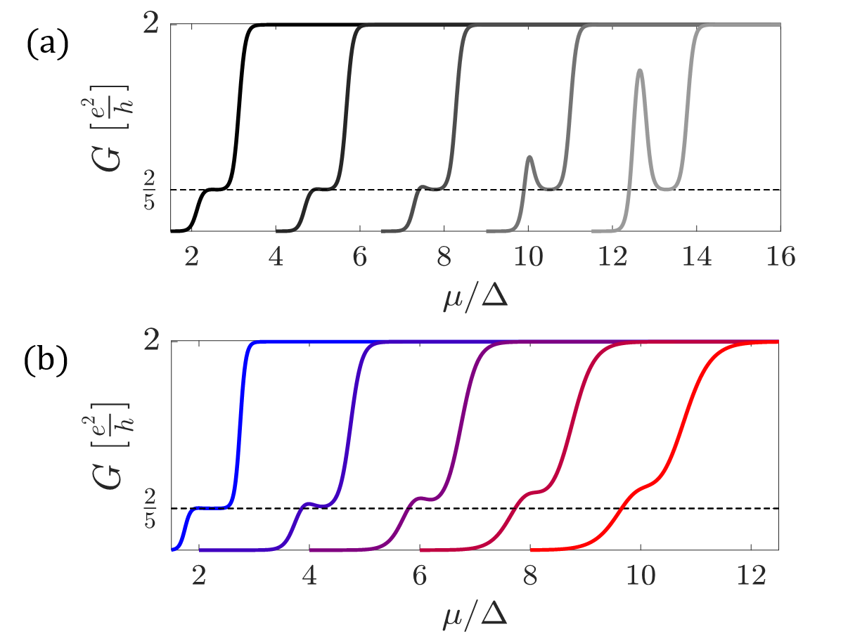
Figure 2: Conductance in a gate-voltage sweep for the time-reversal invariant nano-wire described by the Hamiltonian density $\mathcal{H}_{R}\left(k\right)=\frac{1}{2m}\left(k+\sigma_{z}\alpha\right)^{2}-\mu$, around the filling corresponding with $\left(1,3\right)$. (a) Plateaus at $\frac{T}{\Delta}=0.15$, varying interband separation (left to right) $\frac{\alpha}{\sqrt{2m\Delta}}=1,1.2,1.5,2,2.5$. (b) With $\frac{\alpha}{\sqrt{2m\Delta}}=1.4$ and different temperatures (left to right) $\frac{T}{\Delta}=0.1,0.2,0.3,0.4,0.5$. Plots are shifted horizontally for clarity.

Ultra-low $T$ limit.— Our re-fermionization results cease to be valid for finite system length once the temperature is sufficiently low, i.e., for $T\ll\frac{u}{L}\equiv T_{L}$, which may be understood from the following. Upon re-scaling the bosonic fields, one should in principle also apply the same transformation to the leads, before matching the boundary conditions. Neglecting this step may by justified, in the case where all two-point correlators involved in the current, $\left\langle e^{2i\phi_{g}\left(x,\tau\right)}e^{-2i\phi_{g}\left(x^{\prime},\tau^{\prime}\right)}\right\rangle$, approach their value for a uniform LL. This occurs at $T\gg T_{L}$. In the opposite limit, we may treat the interacting section as a point-like perturbation in the non-interacting leads Ponomarenko and Nagaosa (1998). Using well-known results for such perturbations Kane and Fisher (1992a, b), we find universal power-law behavior of the conductance Sup . Slightly below $T_{L}$, the correction to the universally fractionalized value is

$$G-g\frac{e^{2}}{h}\propto\left(\frac{T_{x}}{T}\right)^{2\left(1-\frac{1}{n_{1}^{2}+n_{2}^{2}}\right)}.$$ (11)

Reducing the energy scale further below $T_{x}\sim T_{L}e^{-\Delta/T_{L}}$, an integer conductance is recovered, behaving much below $T_{x}$ as

$$G-2\frac{e^{2}}{h}\propto\left(\frac{T}{T_{x}}\right)^{2\left(n_{1}^{2}+n_{2}^{2}-1\right)}.$$ (12)

This result is in agreement with Ponomarenko and Nagaosa (1998), who considered the case $n_{1}=n_{2}=1$. Thus, for higher order backscattering processes, the conductance will tend to perfect transmission more sharply. The different $T$-dependent conductance regimes are summarized in Fig. 3.

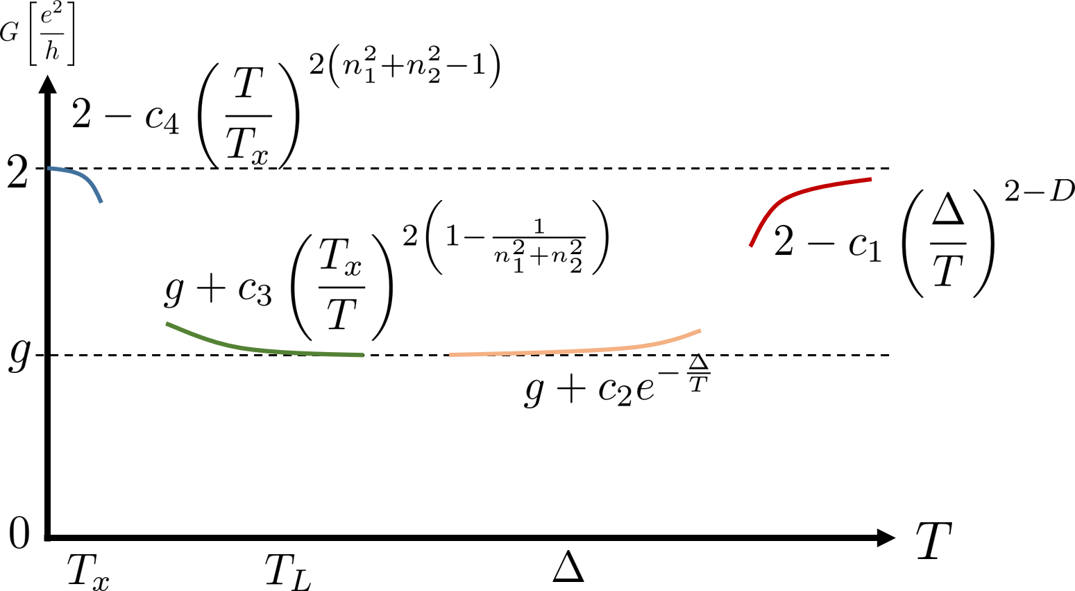
Figure 3: Schematic depiction of the conductance as a function of temperature. At temperatures above $T_{L}$ the behavior is determined by the ratio $\frac{\Delta}{T}$, with an exponentially small correction to the universal fractional value $g$ at low temperatures, and a power-law behavior at high temperatures. Below $T_{L}$, the exponentially small energy scale $T_{x}$ determines the universal power-law of the conductance.

The temperature dependence of the conductance is modified in the presence of a small amount of sharp impurities. These impurities, which are more relevant in the RG sense, will impede the flow of $y^{*}$ to strong coupling and ensure an integer value of the conductance is not reached, even exactly at $T=0$. The qualitative behavior of the conductance in the presence of such impurities, and their effects in the higher temperature limit, are intricate, and depend on the energy scales $\Delta$, $T_{L}$, and the impurity energy scale, see SM, Sec. S.E Sup .

Connection with recent experiments.— The results and discussion above are particularly interesting, as plateaus which are a fraction of $\frac{e^{2}}{h}$ have been recently experimentally observed Gul et al. (2018); Pepper . We conjecture that weak confinement in the lateral direction, a crucial ingredient in obtaining the experimentally observed fractional plateaus, gives rise to the appearance of additional modes, originating in transverse direction quantization (cf. a similar argument in Meyer and Matveev (2009)). Thus, properly tuning a gate, a commensurability condition, which allows $\mathcal{O}_{\lambda}$ to establish itself, may occur, subsequently leading to formation of a fractional plateau. Although according to (6) this would generically lead to $2>g>1$, unlike the reported measurements, a scenario such as in Fig. 1d, where channels may be confined, yet interact strongly throughout the system, result in (7) with $g_{i{\rm c}}<1$, capturing some of the values obtained experimentally. The lateral asymmetry of the 1D channel, which was found to bear great influence on the measurements, may also play some role, as it could lead to an effective SO interaction Moroz and Barnes (1999); Bulgakov and Sadreev (2002). If this is indeed the case, then commensurability may be established between modes of effective opposing helicity Sup . Notice that contrary to Rashba nanowires, we find that that plateaus may form in the absence of magnetic field, in a time reversal conserving fashion. In fact, the most relevant time reversal conserving processes are with $n_{1}=1$ and $n_{2}=3$ leading to the universal value $g=\frac{2}{5}$, was observed without magnetic field Kumar et al. (2018).

The shape of plateaus that we calculated (Fig. 2) fits well to the measurements. Specifically, a conductance peak to the left of the plateau region is often observed. It is a signature of the gate-voltage regime lower than the critical commensurate value, where the conductance should attain its higher, non-fractional value.

Lastly, we comment on the actual values of fractional conductance that were measured. While some reported values may indeed occur in our theoretical model, others are absent, e.g., $\frac{2}{3}$, $\frac{3}{10}$. A plausible explanation is that perhaps some reported plateaus do not necessarily sit at universal values due to finite temperature, cf. Fig. 2b. Moreover, taking into account impurities, or having $T\lesssim T_{L}$, the conductance is expected to be non-universal, albeit maintaining the presence of a chemical potential “window” where the fractional conductance value is stabilized, i.e., a plateau.

Conclusions.— In this work, we have shown that stabilization of fractional two terminal conductance plateaus, which are at a universal fraction of $\frac{e^{2}}{h}$ depending only on band fillings, requires sufficiently strong interactions and tuning of the chemical potentials. In addition to the two-terminal scenario, we also implement our two-band model to fractional Coulomb drag setups, and to cases where some species are confined within the wire. Solving the re-fermionized problem exactly on the generalized Luther-Emery line, we were able to obtain quantitative finite temperature and length corrections to the universal value, as well as the restoration of the integer value of the conductance at ultra small temperatures. This allowed us to suggest a feasible explanation to recent experimental observation of factional conductance plateaus. We expect that further insight into these experiments may be attained from measuring the behavior of the conductance with varying temperatures, and the shot-noise.

Acknowledgments.— We acknowledge enlightening discussion with Karsten Flensberg, Sanjeev Kumar, Tommy Li, Yigal Meir, and Michael Pepper. This work was partially supported by the European Union’s Horizon 2020 research and innovation programme (grant agreement LEGOTOP No 788715), the DFG (CRC/Transregio 183, EI 519/7- 1), and the Israel Science Foundation (ISF) and the Binational Science Foundation (BSF).

Supplemental Material for “Fractional Conductance in Strongly Interacting 1D Systems”

In this supplemental material, we provide technical details for some of the main results of our work, namely the scattering matrix calculations, generalized to a many-band scenario, and the re-fermionized conductance calculations. Additionally, we discuss the consequences of having time-reversal symmetry in the system, some details of the low-$T$ limit, and how the presence of small disorder impacts our findings.

S.A Scattering matrix calculations and many-bands generalization

S.A.1 Conductance

Here we outline the calculation performed in the scattering matrix formalism for a general case of $N$ species of interacting electrons in the 1D system. In the main text, the case of $N=2$ was explored. As mentioned in the main text, we adiabatically attach non-interacting leads to both ends of the system, and define the incoming vector current $\vec{I}=\left(I_{R,1},...,I_{R,N},I_{L,1},...,I_{L,N}\right)^{T}$ with $I_{r,i}=\frac{e}{2\pi}\partial_{t}\varphi_{r}^{i}|_{x=r\infty}$, and similarly the outgoing vector $\vec{O}$. Assuming left-right symmetry in our system, as well as conservation of current, the incoming and outgoing currents can be related by

$$\begin{pmatrix}O_{R}\\ O_{L}\end{pmatrix}=\begin{pmatrix}\mathcal{T}&1-\mathcal{T}\\ 1-\mathcal{T}&\mathcal{T}\end{pmatrix}\begin{pmatrix}I_{R}\\ I_{L}\end{pmatrix},$$ (S1)

with $\mathcal{T}$ a $N\times N$ matrix, and we have separated the current vectors into chiral vectors of length $N$, e.g., $I_{R}=\left(I_{R,1},...,I_{R,N}\right)^{T}$.

Consider the backscattering operator $\left(\psi_{R}^{1\dagger}\psi_{L}^{1}\right)^{n_{1}}\left(\psi_{R}^{2\dagger}\psi_{L}^{2}\right)^{n_{2}}...\left(\psi_{R}^{N\dagger}\psi_{L}^{N}\right)^{n_{N}}$, with $n_{i}$ integers, and negative $n_{i}$ should be interpreted as backscattering in the opposite direction, i.e. $\left(\psi_{R}^{1\dagger}\psi_{L}^{1}\right)^{-\left|n\right|}\equiv\left(\psi_{L}^{1\dagger}\psi_{R}^{1}\right)^{\left|n\right|}$. If for a given $i$ $n_{i}=0$, this species is absent from the backscattering process (though still possibly contributes to the transport). In the language of our bosonization scheme, this operator takes the form

$$\lambda_{N}\cos\left(2\sum_{i}n_{i}\phi_{i}\right),$$ (S2)

and has a scaling dimension (up to corrections due to inter-species forward scattering) $\sim\left(\sum_{i}n_{i}^{2}\right)K$, with $K$ the Luttinger parameter accounting for intra-species electron-electron interactions.

In the limit $\lambda_{N}\rightarrow\infty$ this perturbation pins $\phi_{g}\equiv\frac{\sum_{i}n_{i}\phi_{i}}{\sqrt{\sum_{i}n_{i}^{2}}}$ to a constant value, leading to the boundary condition

$$\sum_{i}n_{i}\partial_{t}\left(\varphi_{L}^{i}-\varphi_{R}^{i}\right)=0,$$ (S3)

inside the interacting section of the wire. The representation of $\phi_{g}$ in terms of $n_{i}$ can be thought of as a normalized vector in $N$-dimensional space, $\phi_{g}=\mathbf{n}\cdot\vec{\phi}$, with $\vec{\phi}=\left(\phi_{1},...,\phi_{N}\right)^{T}$. Notice that $\mathbf{n}^{T}\mathbf{n}=1$. Taken at the opposite ends of the wire, (S3) gives

$$\mathbf{n}^{T}\left(O_{L}-I_{R}\right)=0,\,\,\,\,\mathbf{n}^{T}\left(O_{R}-I_{L}\right)=0,$$

or equivalently,

$$\mathbf{n}^{T}\mathcal{T}\left(I_{L}-I_{R}\right)=0.$$

As this result does not depend on the incoming current vector $\vec{I}$, we find the condition

$$\mathbf{n}^{T}\mathcal{T}=0.$$ (S4)

The remaining gapless modes $\phi_{f,2},...,\phi_{f,N}$ span the $\left(N-1\right)$-dimensional plane perpendicular to $\phi_{g}$, such that $\phi_{f,j}\equiv\mathbf{m}_{j}\cdot\vec{\phi}$, and for all $j$ $\mathbf{m}_{j}\cdot\mathbf{n}=0$. We assume these vectors are normalized as well, $\mathbf{m}_{j}^{T}\mathbf{m}_{j}=1$ for all $j$. These modes are assumed to propagate freely throughout the wire, leading to another $2N-2$ boundary equations, which are written in terms of the current vectors as

$$\mathbf{m}_{j}^{T}\left(O_{R/L}-I_{R/L}\right)=0.$$

Similarly to before, this yields another condition on the $\mathcal{T}$ matrix,

$$\forall j,\,\,\,\,\,\,\,\,\mathbf{m}_{j}^{T}\left(1-\mathcal{T}\right)=0.$$ (S5)

It is easily verifiable that

$$\mathcal{T}=1-\mathbf{n}\mathbf{n}^{T}$$ (S6)

is a solution of (S4),(S5). Since these boundary conditions fully specify how $\mathcal{T}$ operates on a complete basis of the $N$-dimensional space (it is spanned by $\mathbf{n}$ and all the $\mathbf{m}_{j}$ vectors), Eq. (S6) is also the only solution.

The two-terminal conductance may be extracted by imposing a voltage difference between the different sides of the system, which amounts to

$$g=1_{N}^{T}\mathcal{T}1_{N}=N-\frac{\left(\sum_{i}n_{i}\right)^{2}}{\sum_{i}n_{i}^{2}},$$ (S7)

with $1_{N}$ a column vector of ones of length $N$. This result reduces to Eq. (6) of the main text in the case of two fermionic species. Scenarios similar to Fig. 1d may also be considered, by attaching only some of the modes to the voltage leads. The vector $1_{N}$ is replaced by the vector $a_{N}$, which is comprised of ones for the channels attached to the leads, and zeros elsewhere, such that Eq. (S7) is modified to

$$g_{{\rm c}}=N_{a}-\frac{\left(\sum_{i\in a}n_{i}\right)^{2}}{\sum_{i}n_{i}^{2}},$$ (S8)

with $N_{a}$ the number of attached modes and $\sum_{i\in a}$ is a sum over the coefficients of the attached modes only. As an example, for $\mathbf{n}=\left(1,-2,1,-2\right)$, if only the second and fourth modes arrive at the leads, one obtains $g_{{\rm c}}=2-\frac{16}{10}=\frac{2}{5}$.

Some additional examples of fractional conductance coefficients, occurring for the two band ($N=2$) case are given in Table 1.

$\left(n_{1},\left|n_{2}\right|\right)$	$g_{n_{1},-\left|n_{2}\right|}$	$g_{n_{1},\left|n_{2}\right|}$	$g_{12}$	$g_{i{\rm c}}$	$\frac{q^{*}}{e}\left(n_{1},-\left|n_{2}\right|\right)$	$\frac{q^{*}}{e}\left(n_{1},\left|n_{2}\right|\right)$
$\left(1,1\right)$	$2$	$0$	$\frac{1}{2}$	$\frac{1}{2}$	$0$	$1$
$\left(1,2\right)$	$\frac{9}{5}$	$\frac{1}{5}$	$\frac{2}{5}$	$\frac{1}{5}{\rm\,or\,}\frac{4}{5}$	$\frac{1}{5}$	$\frac{3}{5}$
$\left(1,3\right)$	$\frac{8}{5}$	$\frac{2}{5}$	$\frac{3}{10}$	$\frac{1}{10}{\rm\,or\,}\frac{9}{10}$	$\frac{1}{5}$	$\frac{2}{5}$
$\left(1,4\right)$	$\frac{25}{17}$	$\frac{9}{17}$	$\frac{4}{17}$	$\frac{1}{17}{\rm\,or\,}\frac{16}{17}$	$\frac{3}{17}$	$\frac{5}{17}$
$\left(2,3\right)$	$\frac{25}{13}$	$\frac{1}{13}$	$\frac{6}{13}$	$\frac{4}{13}{\rm\,or\,}\frac{9}{13}$	$\frac{1}{13}$	$\frac{5}{13}$

Table 1: Examples of the different fractional transport coefficients. The second and third columns correspond to total momentum conserving ($\mathcal{O}_{{\rm bs}}$) or umklapp-like ($\mathcal{O}_{{\rm um}}$) processes. The fourth column is the drag transconductance. The conductance $g_{i{\rm c}}$ is obtained when $n_{1}$ or $n_{2}$ bands do not reach the voltage leads. The last two columns are the corresponding Fano factors obtained from the tunneling shot-noise (S9).

S.A.2 Tunneling shot-noise

For a system with a finite length, tunneling events of charge between the non-interacting leads may affect the conductance. Such an event is represented by tunneling between adjacent minima of the cosine of (S2). These minima are fixed in the limit $L\rightarrow\infty$, $T=0$. Tunneling between adjacent minima causes a $\frac{\pi}{\sqrt{\sum_{i}n_{i}^{2}}}$ temporal kink in $\phi_{g}$ for the duration of the tunneling. The total charge transferred between the leads can be easily found by integrating the charge current over the time of the tunneling event. Since the charge current is given by

$$j_{c}=\frac{1}{\pi}\partial_{t}\sum_{i}\phi_{i}=\frac{1}{\pi}\partial_{t}\left[\left(\mathbf{n}\cdot 1_{N}\right)\phi_{g}+\sum_{j}\left(\mathbf{m}_{j}\cdot 1_{N}\right)\phi_{f,j}\right],$$

the total fractional charge transferred is

$$q^{*}=\int dtj_{c}=\frac{\sum_{i}n_{i}}{\sum_{i}n_{i}^{2}}e.$$ (S9)

For $V\gg T,T_{L}$, these tunneling events will dominate the dc shot-noise given by Chamon et al. (1995)

$$S\left(\omega\rightarrow 0\right)=2q^{*}I_{t},$$ (S10)

with $I_{t}$ the excess tunneling current in the $\phi_{g}$ channel, $I_{t}=I-\frac{e^{2}}{h}gV$, with $I$ being the total measured current. Thus, we identify $q^{*}$ with the Fano factor of this shot-noise contribution. This result is a many-band generalization of a similar formula obtained in previous works Cornfeld et al. (2015), and gives the same result for the $N=2$ case.

S.B Detailed derivation of the refermionization solution

Let us write the Euclidean action accounting for (3)–(4) as

$$S=\frac{u}{2\pi}\int dxd\tau\left[\mathcal{L}_{f}+\mathcal{L}_{g}+\mathcal{L}_{\mathcal{O}}+\mathcal{L}_{\times}\right],$$ (S11)

with

$$\mathcal{L}_{a}=\phi_{a}\left(-\frac{1}{K_{a}^{2}}\partial_{x}^{2}-\frac{1}{u^{2}}\partial_{\tau}^{2}\right)\phi_{a},$$

for $a=f,g$,

$$\mathcal{L}_{\mathcal{O}}=y\cos\left(2\sqrt{n_{1}^{2}+n_{2}^{2}}\phi_{g}\right),$$

$$\mathcal{L}_{\times}=\frac{1}{K_{\times}^{2}}\partial_{x}\phi_{f}\partial_{x}\phi_{g},$$

and the modified Luttinger parameters

$$K_{f}^{-2}=\frac{1}{2}\left(\frac{1}{K_{+}^{2}}\frac{\left(n_{1}-n_{2}\right)^{2}}{n_{1}^{2}+n_{2}^{2}}+\frac{1}{K_{-}^{2}}\frac{\left(n_{1}+n_{2}\right)^{2}}{n_{1}^{2}+n_{2}^{2}}\right),$$

$$K_{g}^{-2}=\frac{1}{2}\left(\frac{1}{K_{+}^{2}}\frac{\left(n_{1}+n_{2}\right)^{2}}{n_{1}^{2}+n_{2}^{2}}+\frac{1}{K_{-}^{2}}\frac{\left(n_{1}-n_{2}\right)^{2}}{n_{1}^{2}+n_{2}^{2}}\right),$$

$$K_{\times}^{-2}=\frac{n_{1}^{2}-n_{2}^{2}}{n_{1}^{2}+n_{2}^{2}}\left(\frac{1}{K_{-}^{2}}-\frac{1}{K_{+}^{2}}\right).$$

The cross term $\mathcal{L}_{\times}$ should not be neglected here (the way it implicitly was in the scattering matrix calculations), as the boundary conditions for the voltage leads (8) contain $K_{\pm}$, which account for the electrostatic charging of the interacting wire Egger and Grabert (1998). Ignoring $\mathcal{L}_{\times}$would thus be inconsistent with (8) and lead to non-universal asymptotic conductance. By a shift of $\phi_{f}\rightarrow\phi_{f}+Q\phi_{g}$, with $Q$ chosen as

$$Q\equiv\frac{\left(n_{1}^{2}-n_{2}^{2}\right)\left(\frac{1}{K_{+}^{2}}-\frac{1}{K_{-}^{2}}\right)}{\frac{1}{K_{-}^{2}}\left(n_{1}-n_{2}\right)^{2}+\frac{1}{K_{-}^{2}}\left(n_{1}+n_{2}\right)^{2}},$$ (S12)

we find the modified Lagrangian densities

$$\mathcal{L}_{g}+\mathcal{L}_{\mathcal{O}} =\phi_{g}\left(-\left(K_{g}^{-2}+K_{f}^{-2}Q^{2}\right)\partial_{x}^{2}-\frac{1+Q^{2}}{u^{2}}\partial_{\tau}^{2}\right)\phi_{g}$$

$$+y\cos\left(2\sqrt{n_{1}^{2}+n_{2}^{2}}\phi_{g}\right),$$ (S13)

$$\mathcal{L}_{\times} =\frac{2Q}{u^{2}}\partial_{\tau}\phi_{fLL}\partial_{\tau}\phi_{g}.$$ (S14)

Notice that $\mathcal{L}_{f}$ is unaffected by this transformation. As $\mathcal{L}_{\times}$ now vanishes in the static limit, it will henceforth be neglected in the massive $\phi_{g}$ regime. With the shift performed above, we write the current and densities operators using

$$\hat{O}_{+}=\frac{\left[\left(n_{1}+n_{2}\right)+Q\left(n_{2}-n_{1}\right)\right]\hat{O}_{g}+\left(m-n\right)\hat{O}_{f}}{\sqrt{n_{1}^{2}+n_{2}^{2}}},$$

$$\hat{O}_{-}=\frac{\left[\left(n_{1}-n_{2}\right)+Q\left(n_{2}+n_{1}\right)\right]\hat{O}_{g}+\left(m+n\right)\hat{O}_{f}}{\sqrt{n_{1}^{2}+n_{2}^{2}}},$$

with $\hat{O}=\rho,j$. These expressions are plugged in (8) to obtain the boundary equations in terms of the $g$ and $f$ bosonic fields.

Before the re-fermionization step, we rescale the bosonic fields,

$$\tilde{\phi}_{f}=\frac{1}{\sqrt{K_{f}}}\phi_{f},\,\,\,\,\,\tilde{\theta}_{f}=\sqrt{K_{f}}\theta_{f},$$

$$\tilde{\phi}_{g}=\frac{1}{\sqrt{\tilde{K}}}\phi_{g},\,\,\,\,\,\tilde{\theta}_{g}=\sqrt{\tilde{K}}\theta_{g},$$

with $\tilde{K}=\sqrt{\frac{1+Q^{2}}{K_{g}^{-2}+K_{f}^{-2}Q^{2}}}$. At the special line defined by $\tilde{K}=\frac{1}{n_{1}^{2}+n_{2}^{2}}\equiv K^{*}$, the gapped channel describes non-interacting fermions (the $\tilde{f}$ sector is free as well, for any $K_{f}$). The quadratic in fermion operators Hamiltonian may be written as

$$H =\int dx\Psi_{f}^{\dagger}\left[iu\sigma_{z}\partial_{x}\right]\Psi_{f}$$

$$+\int dx\Psi_{g}^{\dagger}\left[iu\sigma_{z}\partial_{x}+\Delta\left(x\right)\sigma_{x}\right]\Psi_{g},$$ (S15)

with$\Psi_{g}=\left(L_{g},R_{g}\right)^{T},\,\,\,\,\,\Psi_{f}=\left(L_{f},R_{f}\right)^{T},$ and the chiral fermionic fields defined as vertex operators of the rescaled bosonic variables, $R_{j}\sim e^{-i\left(\tilde{\phi}_{j}-\tilde{\theta}_{j}\right)},$ $L_{j}\sim e^{i\left(\tilde{\phi}_{j}+\tilde{\theta}_{j}\right)}$. The density and current operators of the two sectors are thus given by

$$\rho_{j}=\Psi_{j}^{\dagger}\Psi_{j},$$ (S16)

$$j_{j}=-u\Psi_{j}^{\dagger}\sigma_{z}\Psi_{j},$$ (S17)

and we may express the boundary conditions in terms of them. Next, we look for solutions for the Schrodinger equation $H\Psi_{j}=E\Psi_{j}$. We find

$$\Psi_{f}\left(E\right)=\begin{pmatrix}\eta_{1}e^{i\frac{E}{u}\left(x-\frac{L}{2}\right)}\\ \eta_{2}e^{-i\frac{E}{u}\left(x+\frac{L}{2}\right)}\end{pmatrix},$$ (S18)

with $\eta_{1/2}$ fermionic operators. Clearly, by using (S16)–(S17), such a solution gives rise to spatially independent forms of $j_{f},\rho_{f}$. Assuming the spatial profile of the gap $\Delta\left(x\right)$ is sufficiently smooth at the connection to the leads, i.e., varies on a length scale greater than $\frac{u}{\Delta}$, we may assume a similar form for the gapped fermions wave function above the gap (as backscattering is suppressed),

$$\Psi_{g}\left(E>\Delta\right)=\begin{pmatrix}\eta_{3}e^{i\frac{\sqrt{E^{2}-\Delta^{2}}}{u}\left(x-\frac{L}{2}\right)}\\ \eta_{4}e^{-i\frac{\sqrt{E^{2}-\Delta^{2}}}{u}\left(x+\frac{L}{2}\right)}\end{pmatrix},$$ (S19)

which again results in spatially uniform charge and current densities. Thus, for $E>\Delta$, we may solve (8) as a set of equations for four position independent variables, and extract

$$j_{c}\left(E>\Delta\right)=\frac{1}{\pi}\delta f.$$ (S20)

For energies below the gap, we find an exponentially decaying solution along the system,

$$\Psi_{g}\left(E<\Delta\right) =\frac{1}{\sqrt{2}}\xi_{1}\begin{pmatrix}1\\ \frac{E-i\kappa u}{\tilde{\Delta}}\end{pmatrix}e^{-\kappa\left(x+\frac{L}{2}\right)}$$

$$+\frac{1}{\sqrt{2}}\xi_{2}\begin{pmatrix}1\\ \frac{E+i\kappa u}{\tilde{\Delta}}\end{pmatrix}e^{\kappa\left(x-\frac{L}{2}\right)},$$ (S21)

with $\kappa\equiv\frac{\sqrt{\Delta^{2}-E^{2}}}{u}$, and fermionic operators $\xi_{1/2}$. Thus, we may express the charge and current operators of the gapped re-fermions as

$$j_{g} =-ue^{-\kappa L}\left(\frac{\kappa u}{\kappa u+iE}\xi_{1}^{\dagger}\xi_{2}+\mathrm{h.c.}\right),$$ (S22)

$$\rho_{g} \left(x=-\frac{L}{2}\right)=\xi_{1}^{\dagger}\xi_{1}+\xi_{2}^{\dagger}\xi_{2}e^{-2\kappa L}+e^{-\kappa L}\left(\frac{\xi_{1}^{\dagger}\xi_{2}}{1-i\frac{\kappa u}{E}}+\mathrm{h.c.}\right),$$ (S23)

$$\rho_{g} \left(x=+\frac{L}{2}\right)=\xi_{1}^{\dagger}\xi_{1}e^{-2\kappa L}+\xi_{2}^{\dagger}\xi_{2}+e^{-\kappa L}\left(\frac{\xi_{1}^{\dagger}\xi_{2}}{1-i\frac{\kappa u}{E}}+\mathrm{h.c.}\right).$$ (S24)

Assuming the non-interacting leads are adiabatically connected to the wire yields an additional boundary condition, $\left\langle R_{g}^{\dagger}\left(-\frac{L}{2}\right)L_{g}\left(\frac{L}{2}\right)\right\rangle=\left\langle\left\langle L_{g}^{\dagger}\left(\frac{L}{2}\right)R_{g}\left(-\frac{L}{2}\right)\right\rangle\right\rangle=0$, such that there is no $2k_{F}$ backscattering in the leads. This amounts to the following relations between the fermionic operators,

$$\xi_{1}^{\dagger}\xi_{1}+\xi_{2}^{\dagger}\xi_{2}=-\frac{\kappa u}{E}\cosh\kappa L\left(i\xi_{1}^{\dagger}\xi_{2}\frac{\kappa u-iE}{\kappa u}+\mathrm{h.c.}\right),$$ (S25)

$$\xi_{2}^{\dagger}\xi_{2}-\xi_{1}^{\dagger}\xi_{1}=\sinh\kappa L\left(\xi_{1}^{\dagger}\xi_{2}\frac{\kappa u-iE}{\kappa u}+\mathrm{h.c.}\right).$$ (S26)

Manipulating Eqs. (S22)–(S26), we may finally relate the current $j_{g}$ to the difference in densities between the ends of the wire,

$$j_{g} =u\frac{\Delta^{2}-E^{2}}{2\Delta^{2}\sinh^{2}\kappa L}\left(\rho_{g}\left(x=+\frac{L}{2}\right)-\rho_{g}\left(x=-\frac{L}{2}\right)\right).$$ (S27)

We may now solve once again (8) as a set of linear equations, but now the variables are $\rho_{f},j_{f},\rho_{g}\left(x=\pm\frac{L}{2}\right)$. Straightforward calculation yields $j_{f}$ and $\rho_{g}$, and thus $j_{g}$. We plug them into the total charge current, given in the “shifted” basis by

$$j_{c}=\frac{\left[\left(n_{1}+n_{2}\right)+Q\left(n_{2}-n_{1}\right)\right]j_{g}+\left(n_{2}-n_{1}\right)j_{f}}{\sqrt{n_{1}^{2}+n_{2}^{2}}},$$ (S28)

and we finally obtain after some elaborate yet straightforward manipulations,

$$j_{c}\left(E<\Delta\right)=\frac{1}{2\pi}\delta f\frac{\left(n_{2}-n_{1}\right)^{2}+2\chi}{n_{1}^{2}+n_{2}^{2}+\chi},$$ (S29)

with the non-universal factor $\chi=\frac{\Delta^{2}-E^{2}}{2\Delta^{2}\sinh^{2}\kappa L}\left(K_{-}^{2}\left(n_{1}-n_{2}\right)^{2}+K_{+}^{2}\left(n_{1}+n_{2}\right)^{2}\right)$. For low enough temperatures, and in the limit $\kappa L\rightarrow 0$, one finds $\chi\rightarrow\infty$, and an integer conductance of $g=2$ is restored. For the opposite limit, $\kappa L\rightarrow\infty$, one recovers the universal value, Eq. (6). The dependence of the conductance on temperature, chemical potential (i.e., the distance from the commensurability point), and voltage, are encapsulated within the $\delta f$ dependence.

Combining Eqs. (S20),(S29), integrating over energy, and restoring units, we may calculate the two-terminal conductance for arbitrary temperature and system length. An example is shown in Fig. S1 for the case of $\left(1,3\right)$, which was considered in Fig. 2. Additionally, we show two cuts with constant temperature or length, showing the power-law behavior at small $L$ and high $T$.

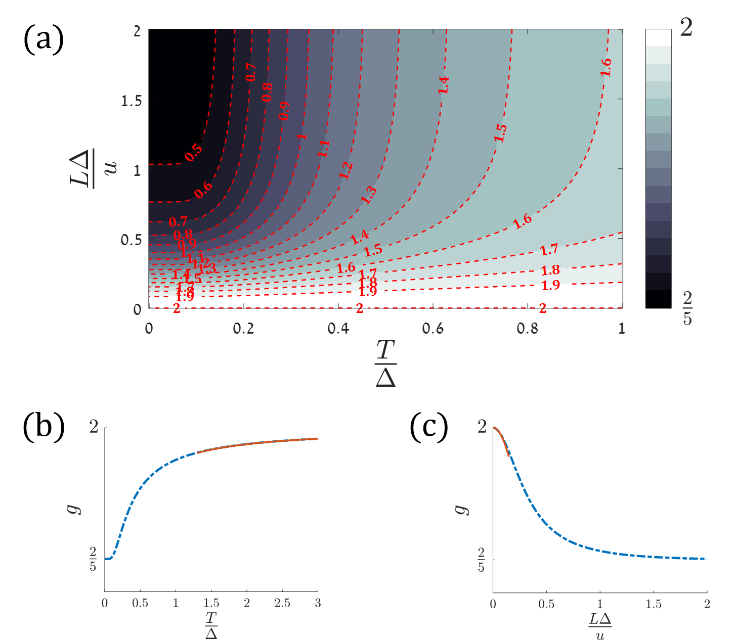
Figure S1: Calculation of the conductance (in units of $\frac{e^{2}}{h}$) for the case of $\left(n_{1},n_{2}\right)=\left(1,3\right)$. (a) Conductance as a function of $T$ and $L$. (b) Dashed blue line: a cut with constant $\frac{L\Delta}{u}=1.3$; solid red line: power-law fit with $2-g\propto\left(\Delta/T\right)$. (c) Dashed blue line: a cut with constant $\frac{T}{\Delta}=0.15$; solid red line: power-law fit with $2-g\propto\left(L\Delta/u\right)^{2}$. All calculations were made with the chemical potential exactly at the $\left(1,3\right)$ commensurability point.

S.C Time-reversal invariant systems

Let us consider a system comprised of two one-dimensional channels of opposite helicities, strongly interacting with one another. The helicity need not necessarily correspond to the spin itself, but to a general pseudo-spin degree of freedom, which will be denoted as $\uparrow/\downarrow$ for convenience. We number each helical channel by $1,2$ , as in the main text, corresponding to the mapping of the chiral fermionic operators

$$\psi_{R}^{1}\leftrightarrow\psi_{R,\uparrow},\,\,\,\,\,\psi_{L}^{1}\leftrightarrow\psi_{L,\downarrow},$$

$$\psi_{R}^{2}\leftrightarrow\psi_{R,\downarrow},\,\,\,\,\,\psi_{L}^{2}\leftrightarrow\psi_{L,\uparrow}.$$

By applying different chemical potentials to the two helical channels, the results we obtained in the main text may be applied to such a system.

The presence of time-reversal symmetry modifies the allowed integers that go into the operator $\mathcal{O}_{\lambda}$. To see this, consider that under time-reversal the chiral fermionic operators transform as

$$\psi_{R,\downarrow}\rightarrow\psi_{L,\downarrow},\,\,\,\,\,\psi_{L,\downarrow}\rightarrow-\psi_{R,\downarrow},\,\,\,\,\psi_{L,\uparrow}\rightarrow\psi_{R,\downarrow},\,\,\,\,\,\psi_{R,\downarrow}\rightarrow-\psi_{L,\uparrow}.$$ (S30)

Thus, one finds that $\mathcal{O}_{\lambda}$ is time-reversal invariant only if $\left(n_{1}+n_{2}\right)$ is an even integer.

This scenario may be realized in two different ways, depicted in Fig. S2. (i) Using a narrow sample of a two-dimensional topological insulator (TI), with width $d$ much greater than the characteristic correlation length $\xi$, with different gate voltages applied to the different edges, as to achieve the fractional commensurability of the Fermi momenta. (ii) Constructing a TI-Insulator-TI heterostructure, with different top and bottom gates, or different doping for the two topologically non-trivial layers. In the two scenarios one must ensure that the distance between the different edge states is such that strong electron-electron interactions may take place. Alternatively, the physics of a Rashba nano-wire may be considered.

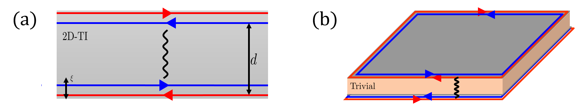
Figure S2: More robust TR symmetric setups using 2D-TIs. (a) Edge states of a thin 2D-TI, with its edges kept in different chemical potential. (b) Edge states of two 2D-TIs with different helicities separated by a trivial insulator are governed by the same Hamiltonian.

S.C.1 Rashba nanowire

The model for a spinfull 1D system with Rashba type spin-orbit coupling (RSO) is captured by the Hamiltonian density

$$\mathcal{H}_{R}\left(k\right)=\frac{k^{2}}{2m}+\mu+\alpha\sigma^{z}k+E_{{\rm Z}}\sigma^{y},$$ (S31)

with $k$ the wave vector, $\alpha$ the RSO strength, $E_{{\rm Z}}$ the Zeeman energy, and $\sigma^{i}$ the Pauli matrices acting on the electrons spin degree of freedom. At $E_{{\rm Z}}=0$, Eq. (S31) describes two copies of parabolic dispersion corresponding to the value of $\sigma_{z}$, shifted in momentum space by the RSO. Focusing on the regime below the energy at which the two bands cross, we linearize the spectrum to obtain the chiral fermion modes, resulting in a system with two channels of opposite helicity, as discussed above.

Previous studies of fractional helical wires Oreg et al. (2014); Aseev et al. (2018) discussed processes analogous to $\left(n,n+1\right)$ backscattering, which inherently break time-reversal symmetry and are only generated in the presence of a finite magnetic field with finite Zeeman energy $E_{{\rm Z}}$. Our treatment generalizes those results to a variety of commensurate filling factors, given by $\nu\equiv\frac{k_{F}}{\alpha m}=\frac{n_{1}-n_{2}}{n_{1}+n_{2}}$. We find that the lowest order non-trivial time-reversal invariant fractional phase occurs at $\left(1,3\right)$, or $\nu=\frac{1}{2}$, with a novel fractional conductance $g=\frac{2}{5}$. A fractional conductance value of $\frac{1}{5}$, found to be the most relevant in the time-reversal breaking model, may still be obtained for the filling factor $\nu=\frac{1}{3}$, but it requires a higher order $\left(2,4\right)$ process for its gap to be established in the system, and thus stronger interactions.

S.D Ultra-low $T$ limit

Our re-fermionization results cease to be valid for finite system length once the temperature is sufficiently low, i.e., for $T\ll\frac{u}{L}\equiv T_{L}$. This may be understood from the following. Upon rescaling the bosonic fields, one should in principle also apply the same transformation to the voltage leads, before matching the boundary conditions. Neglecting this step may by justified, in the case where all two-point correlators involved in the current, $\left\langle e^{2i\phi_{g}\left(x,\tau\right)}e^{-2i\phi_{g}\left(x^{\prime},\tau^{\prime}\right)}\right\rangle$, approach their value for a uniform LL. This occurs at $T\gg T_{L}$. In the opposite limit, we have to treat the interacting section as a point-like perturbation in the non-interacting Fermi liquid which comprises the leads Ponomarenko and Nagaosa (1998). The corresponding Hamiltonian for $\phi_{g}$ in our regime of interest, $\Delta>T,T_{L}$, is given by

$$H_{L}=\frac{u}{2\pi}\int dx\left[\left(\partial_{x}\phi_{g}\right)^{2}+\left(\partial_{x}\theta_{g}\right)^{2}+y^{*}\cos\left(\frac{2\theta_{g}}{\sqrt{n_{1}^{2}+n_{2}^{2}}}\right)\delta\left(x\right)\right],$$ (S32)

with the new parameter $y^{*}\approx\frac{T_{L}}{u\sinh^{2}\left(\frac{\Delta}{u}L\right)}$ Ponomarenko and Nagaosa (1998). Notice that $y^{*}$ is exponentially small in $\frac{\Delta}{T_{L}}$. Eq. (S32) is written in the strong interaction limit, where $y^{*}$ represents a tunneling event between two semi-infinite Luttinger liquids. The perturbation $y^{*}$ is clearly relevant in an RG sense, ensuring it reaches the strong coupling limit at low enough temperatures $T<t\left(\frac{uy^{*}}{t}\right)^{\frac{n_{1}^{2}+n_{2}^{2}}{n_{1}^{2}+n_{2}^{2}-1}}\equiv T_{x}$. At $T=0$ this sector becomes perfectly transmitting, and a total conductance of $2\frac{e^{2}}{h}$ is restored. The Hamiltonian (S32) allows us to find power-law behavior in the deviations from the universal fractional conductance value (6) in the regime $T_{x}\ll T<T_{L}$. Mapping the problem into that of a strong impurity in an interacting LL would reveal the perturbative (in $y^{*}$) result Kane and Fisher (1992a, b)

$$G-g\frac{e^{2}}{h}\propto\left(\frac{T_{x}}{T}\right)^{2\left(1-\frac{1}{n_{1}^{2}+n_{2}^{2}}\right)}.$$ (S33)

By examining the dual model of (S32), which has the dual perturbatively small sine-Gordon term containing $\phi_{g}$, the power-law deviation from perfect transmission around $T=0$ is similarly recovered,

$$G-2\frac{e^{2}}{h}\propto\left(\frac{T}{T_{x}}\right)^{2\left(n_{1}^{2}+n_{2}^{2}-1\right)}.$$ (S34)

S.E Effect of impurities

The 1D system we describe in this work is generally not protected from the presence of disorder and impurity scattering. We thus explore under what conditions do such elements spoil the fractional two terminal conductance and to what extent. In the regime where the scattering mean-free-path is comparable to the system size it is sufficient to consider the effect of a single impurity scattering center.

Backscattering of a single particle in the $i$ fermionic channel is described by an operator $\mathcal{B}_{i}\sim y_{{\rm imp}}\cos 2\phi_{i}$. Its scaling dimension, $\frac{1}{2}\left(K_{+}+K_{-}\right)$, will generically be smaller than one (making it relevant in the RG sense) when $\mathcal{O}_{\lambda}$ is relevant, hence the lack of protection mentioned. However, since the impurity is localized in space, whereas $\mathcal{O}_{\lambda}$ operates along the entire system, the latter may grow much faster under the RG flow, and reach strong coupling first. This is our regime of interest, since it will lead to clear signatures of the partially gapped state. By very crudely estimating $K_{+}\approx K_{-}\equiv K$, this happens for $K<\left(n_{1}^{2}+n_{2}^{2}-1\right)^{-1}$, i.e., repulsive interactions substantially stronger compared to the interaction required to achieve the situation when the dimension of the operator ${\cal O}_{\lambda}$, $D<2$, which is equivalent to $K<2\left(n_{1}^{2}+n_{2}^{2}\right)^{-1}$. Notice that once $\lambda\rightarrow\infty$, $\phi_{g}$ “freezes out” , causing $\mathcal{B}_{i}$ to become even more relevant as its dimension effectively becomes $D_{{\rm imp}}=\left(1-\frac{n_{i}^{2}}{n_{1}^{2}+n_{2}^{2}}\right)K_{f}$.

We now have two different temperature scales in our problem: $T^{*}=\Delta$, the gap originating in $\mathcal{O}_{\lambda}$ , and $T_{f}$, associated with the RG flow of $\mathcal{B}_{i}$, with $T_{f}<T^{*}$ assumed. For $T\gg T^{*}$, the impurity has an insignificant effect and the power-law correction to $2e^{2}/h$ are as in (10). At the vicinity of $T^{*}$ and below it, the conductance settles at the fractional result (6), with exponentially small corrections. As the temperature is lowered even further, the impurity scattering begins to hinder the conductance, until completely gapping out $\phi_{f}$ as well as $\phi_{g}$ at $T\ll T_{f}$. At these very low temperatures, one must start considering the additional energy scale $T_{L}$, and the picture becomes much more complicated. We will henceforth assume for simplicity that the impurity acts simultaneously on both the original channels, $\phi_{1},\phi_{2}$.

If $T_{f}<T_{L}<T^{*}$, the impurity never reaches the strong coupling regime. The impurity contributes a small power-law correction to the conductance, which behaves as $\left(\frac{T_{f}}{T}\right)^{2\left(1-D_{{\rm imp}}\right)}$ above $T_{L}$, and remains a temperature-independent constant below $T_{L}$.

On the other hand, in the regime $T_{L}<T_{f}<T_{*}$, the conductance for temperatures below $T_{f}$ yet significantly above $T_{L}$ will vanish with a non-universal power-law, as $\left(\frac{T}{T_{f}}\right)^{2\left(1-\frac{1}{D_{{\rm imp}}}\right)}$. Once again, below $T_{L}$ the small conductance due to the strong impurity, will remain constant.

Lastly, we note that $T_{f}$ may be “pushed down” to lower temperatures, such that the intermediate temperature regime with conductance very closed to its fractional universal value is greatly expanded, if the 1D system consists of time-reversal (TR) symmetry protected edge states of a 2D topological insulator (e.g., tungsten ditelluride Fei et al. (2017); Wu et al. (2018)) of opposite helicities. Prohibiting single particle backscattering, operators of the order $\sim y_{{\rm imp}}\cos 4\phi_{i}$ or higher may be relevant. The scenario in which $\phi_{g}$ is gapped out before the impurity reaches its strong coupling regime is now roughly given by $K<\left(n_{1}^{2}+n_{2}^{2}-4\right)^{-1}$, i.e., we require much weaker interaction strengths for our regime of interest. The value of $T_{f}\propto y_{{\rm imp}}^{\frac{1}{1-D_{{\rm imp}}}}$ is significantly reduced in this case, since $D_{{\rm imp}}=4\left(1-\frac{n_{i}^{2}}{n_{1}^{2}+n_{2}^{2}}\right)K_{f}$ is four times larger compared to the non-time-reversal-protected system, and the vanishing conductance power-laws are modified accordingly.