Unsupervised Grounding of
Plannable First-Order Logic Representation from Images

Abstract

Recently, there is an increasing interest in obtaining the relational structures of the environment in the Reinforcement Learning community. However, the resulting “relations” are not the discrete, logical predicates compatible with the symbolic reasoning such as classical planning or goal recognition. Meanwhile, Latplan (?) bridged the gap between deep-learning perceptual systems and symbolic classical planners. One key component of the system is a Neural Network called State AutoEncoder (SAE), which encodes an image-based input into a propositional representation compatible with classical planning. To get the best of both worlds, we propose First-Order State AutoEncoder, an unsupervised architecture for grounding the first-order logic predicates and facts. Each predicate models a relationship between objects by taking the interpretable arguments and returning a propositional value. In the experiment using 8-Puzzle and a photo-realistic Blocksworld environment, we show that (1) the resulting predicates capture the interpretable relations (e.g., spatial), (2) they help to obtain the compact, abstract model of the environment, and finally, (3) the resulting model is compatible with symbolic classical planning.

1 Introduction

Recent success in the latent space classical planning (?, Latplan) shows a promising direction for connecting the neural perceptual systems and the symbolic AI systems. Latplan is a straightforward system built upon a state-of-the-art Neural Network (NN) framework (Keras, Tensorflow) and Fast Downward classical planner (?). It builds a set of propositional state representation from the raw observations (e.g., images) of the environment, which can be used for classical planning as well as goal recognition (?). However, Latplan still contains many rooms for improvements in terms of the interpretability and the scalability which are trivially available in the symbolic systems. An instance of such limitations of Latplan is that the reasoning is performed on a propositional level, missing the ontological commitment of the first-order logic (FOL) that the world comprises objects and their relations (?).

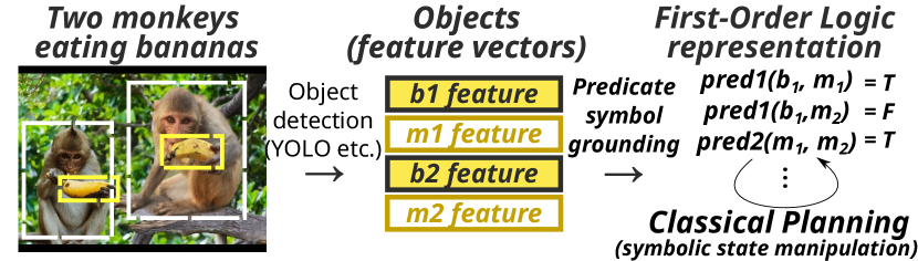
Figure 1: Predicate symbol grounding (PSG) process for identifying the predicates and obtaining the first-order logic (FOL) representation of the environment for symbolic reasoning. In this example, an anonymous binary predicate pred₁ can be interpreted by humans as something like eating$(\textit{object},\textit{subject})$.

FOL is a structured representation, which offers some extent of interpretability compared to the factored representation of the propositional logic formula (?). Even if the predicate symbols discovered by a Predicate Symbol Grounding system (Fig. 1) are machine-generated anonymous symbols (not the human-originated symbols assigned by manual tagging), the structures help humans interpret the meaning of the relations from the several instances of the argument list (objects) that make the predicate true. For example, when two propositions pred(0,1) and pred(1,2) are true, we can guess the meaning of pred as +1, or given pred(monkey, banana) being true, the meaning of pred would be something like eating or holding. This is impossible in a propositional representation where only the variable indices and the truth values are known.

In this paper, we propose First-Order State AutoEncoder (FOSAE, Fig. 5), a NN architecture which, given the feature vectors of the objects in the environment, automatically learns to identify a set of predicates (relations) as well as to select the appropriate objects as the arguments for the predicates. The resulting representation is compatible with classical planning. We do not address the object recognition problem, whose task is to extract the object entities from a raw observation. We instead assume that an external system has already extracted the objects and converted them into the feature vectors, given the recent success of object detection methods like YOLO (?) in image processing. While FOSAE is in principle data-format (e.g., images, text) independent, we focus on the visual input in this paper.

FOSAE provides a higher-level generalization and the more compact model by adding a constraint that the extracted relations are common to multiple tuples of objects. Ideally, predicates model the commonalities between the multiple instantiations of its arguments, rather than rote learning some unrelated combinations. In order to discover such predicates, our framework ensures that a single predicate is applied to the different arguments within the same observation. Otherwise, the network may choose to apply them to the same or the very narrow combinations of arguments in every observation, resulting in an inflexible predicate that merely remembers some combinations. Since the model utilizes the same weights multiple times over the different arguments, this also reduces the number of weight parameters required to model the environment.

The rest of this paper is organized as follows. Sec. 2 reviews and discusses the issues in the existing work on the relational structures for NNs. Sec. 3 explains Latplan, the key target of the enhancement proposed in this paper, as well as the backgrounds for NNs such as attention that plays a key role in extracting the argument list of the predicates. Sec. 4 discusses the process for learning the first-order logic representation of the environment, and Sec. 5 proposes First-Order State AutoEncoder (FOSAE), the architecture that performs the process. In Sec. 6, we conduct experiments on a toy 8-puzzle domain to address the interpretability and generalization of FOSAE and its compatibility to symbolic PDDL planning systems. In Sec. 7.2, we demonstrate the ability of FOSAE on a photo-realistic Blocksworld domain.

2 Background

One of the early work on learning the relations between object symbols includes Linear Relational Embedding (?), which is learned from the tuples of relations and objects in a supervised manner. Supervision makes the resulting representation parasitic to human knowledge; thus it does not fully solve the knowledge acquisition bottleneck. Also, their approach is limited to binary relations.

Recently, there are increasing interest in the effectiveness of finding “relations” in Deep Reinforcement Learning (?, DRL) community. Deep Symbolic RL (?) showed that a hand-crafted “common sense prior” (e.g., proximity) accelerates DRL. Relation Networks (?) combine two elements in the feature maps of a convolutional neural network (?) and output real values. Deep Relational RL (?) combines Relation Networks and attention-based message passing. Relational Inductive Bias (?) shows that DRL is enhanced by a hand-crafted, explicit graph representation of the input and the Graph Neural Networks (?). Relational Neural Expectation Maximization (?) enumerates pairs of objects to model the relations in the environment for common-sense physics modeling. Neural theorem proving systems (?; ?; ?) learn to reason about logical relations. In this paper, we address the following issues in these work:

Human Supervision. Providing a relational dataset as an input (as in (?) and neural theorem proving), or a probabilistic logic program containing predicate symbols which defines a network, exhibits the knowledge acquisition bottleneck as the predicates are grounded by humans and thus the system relies on human knowledge.

Compatibility with the symbolic systems. Relational structures in existing work do not return explicit boolean values even when the environment is deterministic, fully observable and discrete. This makes them incompatible with symbolic systems such as classical planners or goal recognition. Ideally, systems should guarantee that a discrete environment is represented in a discrete form, and numeric variables (such as those handled by numeric planner) should be introduced only when necessary.

Interpretability. Some networks use real-valued soft attentions (probability) to model the objects that take part in a relation, which are similar to the predicate arguments. However, the relations resulted from soft attentions are hard to interpret due to the ambiguity, e.g., “Bob has-a ‘50% dog and 50% cat”’ in a “has-a” relation. Continuous outputs of the relational structures are also difficult to interpret.

Scalability for higher arities. Some work assumes the binary relations and enumerates $O(N^{2})$ pairs for $N$ objects. The explicit structure is impractical for larger arities $A$ because the network size $O(N^{A})$ increases exponentially.

Furthermore, empirical, direct evidence that the “relations” are indeed necessary for modeling the environment is missing from the literature. In some previous work, relational structures are embedded inside a reinforcement learning framework, and they showed that such structures had improved the RL performance. However, this is merely a necessary condition rather than a sufficient condition because, in model-free RL, the policy and the representation are learned at once, making it hard to tell whether (1) the network is just numerically faster to converge (similar to skip connections or other techniques) or (2) it models the environment better and therefore it learns the good policy.

3 Preliminaries

We denote an array (either a vector or a matrix) in bold, such as ${\bm{x}}$, and denote its elements or rows with a subscript, e.g., when ${\bm{x}}\in\mathbb{R}^{n\times m}$, the second row is ${\bm{x}}_{2}\in\mathbb{R}^{m}$.

Symbol grounding is an unsupervised process of establishing a mapping from huge, noisy, continuous, unstructured inputs to a set of compact, discrete, identifiable (structured) entities, i.e., symbols (?; ?; ?; ?). PDDL (?) has six kinds of symbols: Objects, predicates, propositions, actions, problems, and domains. Each type of symbol requires its own mechanism for grounding. For example, the large body of work in the image processing community on recognizing objects (e.g., faces) and their attributes (male, female) in images, or scenes in videos (e.g., cooking) can be viewed as corresponding to grounding the object, predicate and action symbols, respectively.

Classical planners such as FF (?) or FastDownward (?) takes a PDDL model as an input, which specifies the state representation, the initial state, the goal condition and the transition rules in the form of the first-order logic formula, and returns an action sequence that reaches the goal state from the initial state. In contrast, Latplan (?) is a framework for domain-independent image-based classical planning. It learns the state representation as well as the transition rules entirely from the image-based observation of the environment with deep neural networks and solves the problem using a classical planner. The system was shown to solve various puzzle domains, such as 8-puzzles or Tower of Hanoi, which are presented in the form of noisy, continuous visual depiction of the environment. Latplan addresses two of the six types of symbols, namely propositional and action symbols.

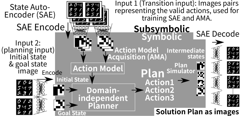
Figure 2: Classical planning in latent space: It uses the learned State Autoencoder (Fig. 3) to convert pairs of images $(pre,suc)$ to symbolic transitions, from which the AMA component generates an action model. It also encodes the initial and goal state images into symbolic initial/goal states. A classical planner finds the symbolic solution plan. Finally, intermediate states in the plan are decoded back to a human-comprehensible image sequence.

Latplan takes two inputs. The first input is the transition input $Tr$, a set of pairs of raw data. Each pair $tr_{i}=(pre_{i},suc_{i})\in Tr$ represents a transition of the environment before and after some action is executed. The second input is the planning input $(i,g)$, a pair of raw data, which corresponds to the initial and the goal state of the environment. The output of Latplan is a data sequence representing the plan execution that reaches $g$ from $i$. While the original paper used an image-based implementation (“data” = raw images), the type of data is arbitrary as long as it is compatible with neural networks.

Latplan works in 3 phases. In Phase 1, a State Autoencoder (SAE) (Fig. 3) learns a bidirectional mapping between raw data (e.g., images) and propositional states from a set of unlabeled, random snapshots of the environment, in an unsupervised manner. The $Encode$ function maps images to propositional states, and $Decode$ function maps the propositional states back to images. After training the SAE from ${\left\{pre_{i},suc_{i}\ldots\right\}}$, it applies $Encode$ to each $tr_{i}\in Tr$ and obtain $(Encode(pre_{i}),$ $Encode(suc_{i}))=$ $(s_{i},t_{i})=$ $\overline{tr}_{i}\in\overline{Tr}$, the symbolic representations (latent space vectors) of the transitions.

In Phase 2, an Action Model Acquisition (AMA) method learns an action model from $\overline{Tr}$ in an unsupervised manner. The original paper proposed two approaches: AMA₁ is an oracular model which directly generates a PDDL without learning, and AMA₂ is a neural model that approximate AMA₁ by learning from examples.

In Phase 3, a planning problem instance is generated from the planning input $(i,g)$. These are converted to symbolic states by the SAE, and the symbolic planner solves the problem. For example, an 8-puzzle problem instance consists of an image of the start (scrambled) configuration of the puzzle ($i$), and an image of the solved state ($g$).

Since the intermediate states comprising the plan are SAE-generated latent bit vectors, the “meaning” of each state (and thus the plan) is not clear to a human observer. However, in the final step, Latplan obtains a step-by-step, human-comprehensive visualization of the plan execution by $Decode$’ing the latent bit vectors for each intermediate state. This is the reason the bidirectionality of the mapping is required in this framework.

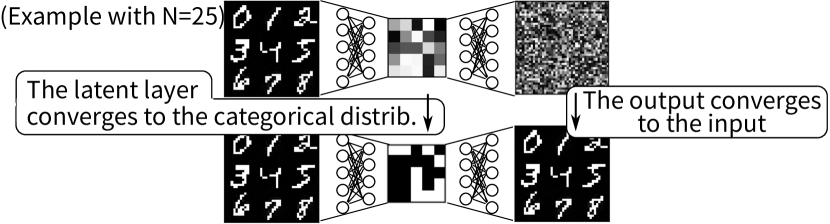
Figure 3: State AutoEncoder, a Variational AutoEncoder (?) using Gumbel-Softmax (?) reparametrization in its latent layer.

The key concept of the SAE in Latplan is the use of Gumbel-Softmax (?, GS) activation function. The output of GS (latent representation) converges to a 1-hot vector of $M$ categories. This allows the SAE to obtain a discrete binary representation by setting $M$=2 and Latplan uses it for classical planning. The output of a single Gumbel-Softmax unit $GS(\bm{\pi})={\bm{z}}\in[0,1]^{M}$ is a one-hot vector representing $M$ categories, e.g., when $M=2$ the categories can be seen as ${\left\{\text{false},\text{true}\right\}}$ and ${\bm{z}}={\left(0,1\right)}$ represents “true”. (Note: There is no explicit meaning assigned to each category.) The input $\bm{\pi}\in[0,1]^{M}$ is a class probability vector, e.g., ${\left(.2,.8\right)}$. Gumbel-Softmax is derived from Gumbel-Max technique (?, Eq. 1) for drawing a categorical sample

$$z_{i} =\textbf{if}\ (i\ \text{is}\ \arg\max_{i}(g_{i}+\log\pi_{i}))\ \textbf{then}\ 1\ \textbf{else}\ 0$$ (1)

$$z_{i} =\text{Softmax}((g_{i}+\log\pi_{i})/\tau).$$ (2)

from $\bm{\pi}$ where $g_{i}$ is a sample drawn from $\text{Gumbel}(0,1)=-\log(-\log u)$ where $u=\text{Uniform}(0,1)$ (?). Gumbel-Softmax approximates the argmax with a Softmax to make it differentiable (Eq. 2). “Temperature” $\tau$ controls the magnitude of approximation, which is annealed to 0 by a certain schedule. The output ${\bm{z}}$ converges to a discrete one-hot vector when $\tau\rightarrow 0$.

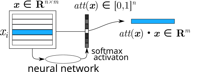
Figure 4: An attention mechanism selecting an $m$-dimensional vector out of $n$ vectors.

Attention is a recent mechanism that enhances the performance of neural network for various cognitive tasks including machine translation (?), object recognition (?), image captioning (?), and Neural Turing Machine (?). Its fundamental idea is to learn an attention function that extracts a single element from multiple elements. The function is represented as a neural network and is trained unsupervised. Typically, the output is activated by a Softmax, which normalizes the sum to 1. The function can be formulated as $\textit{att}({\bm{x}})={\bm{a}}$, where ${\bm{x}}\in\mathbb{R}^{n\times m}$ is a set of $n$ elements ${\bm{x}}=({\bm{x}}_{1},\ldots{\bm{x}}_{n})$, ${\bm{x}}_{i}\in\mathbb{R}^{m}$ and ${\bm{a}}=(a_{1}\ldots a_{n})\in[0,1]^{n}$ satisfies $\sum_{i}a_{i}=1$. It can extract an element ${\bm{x}}_{i}$ of ${\bm{x}}$ using a dot product ${\bm{a}}\cdot{\bm{x}}$. For example, if ${\bm{x}}=((2,0),(3,3),(1,2))$ and ${\bm{a}}={\left(0,0.9,0.1\right)}$, ${\bm{a}}\cdot{\bm{x}}=(2.8,2.9)$, which almost extracts $(3,3)$.

4 High-Level Overview

In order to find a first-order logic representation of the environment from raw data, we perform the following processes (Fig. 1): (1) Object detection identifies and extracts a set of regions from the raw data that contain objects. (2) Predicate symbol grounding (PSG) finds the boolean functions that take several object feature vectors as the arguments.

While both processes are nontrivial, there are significant advances in (1) recently. Object recognition in computer vision (?, YOLO) or named entity (noun / “objects”) recognition (?; ?) in Natural Language Processing, are both becoming increasingly successful. In this paper, therefore, we do not address (1) and use a dataset that is already segmented into image patches and bounding boxes. In principle, we could extract the object vectors with these external systems.

Next, PSG identifies a finite set of boolean functions (predicates) from the feature input, by learning to select the argument list from the input and detecting the common patterns between the objects that define a relation. As a result, we obtain the first-order logic representation of the input as a list of FOL statements such as pred₂(obj₁, obj₂)=true, where the system automatically learns to extract the arguments from the inputs, and also decides the semantics of the predicates by itself, in an unsupervised manner.

While some might worry about the interpretability of the predicates with unknown semantics and its compatibility to the existing knowledge base based on human-made symbols, full autonomy is a valuable option that is orthogonal to the interpretability. While interpretability is essential in the normal operations of, e.g., space exploration applications, autonomy would be critical in an emergency situation. If a system lost contact to the human operators in a unknown environment, it must learn a new representation online (Imagine being abducted by an alien spaceship with shiny walls everywhere! A more realistic example is falling into an underground cave). Moreover, a typical knowledge base is incompatible with raw observations such as images.

5 First-Order State AutoEncoder

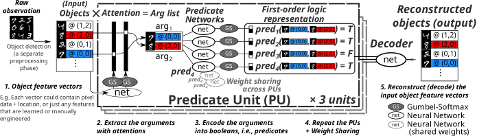
Figure 5: A First-Order State AutoEncoder (FOSAE) with $P=4$ predicates, arity $A=2$, and $U=3$ Predicate Units. In this example, a feature vector consists of the pixel values and the $(x,y)$ location of an 8-Puzzle tile.

We now introduce the core contribution of this paper, First-Order State AutoEncoder (FOSAE, Fig. 5), a neural architecture which performs PSG and obtains a representation compatible with symbolic reasoning systems such as classical planners.

(Fig. 5, 1) Overall, the system follows the autoencoder architecture that takes feature vectors of multiple objects in the environment as the input and reconstructs them as the output. The form of the feature vector for each object is entirely problem/environment dependent: It could be a hand-crafted feature vector, a flattened vector of the raw pixel values for the object, or a latent space vector automatically generated from the image array by an additional feature learning system (such as an autoencoder). Let ${\bm{x}}_{n}\in\mathbb{R}^{F}$ be a $F$-dimensional feature vector representing each object and ${\bm{x}}=({\bm{x}}_{1},\ldots{\bm{x}}_{N})\in\mathbb{R}^{N\times F}$ be the input matrix representing the set of $N$ objects.

FOSAE consists of multiple instances of Predicate Unit, a unit that (1) learns to extract an argument list from the input and (2) computes the boolean values of the predicates given the extracted argument list. The number of units $U$, the arity of predicates $A$ and the number of predicates $P$ are hyperparameters which should be sufficiently large so that the network can encode enough information into a boolean vector and then reconstruct the input. If the network does not converge into a sufficiently low reconstruction loss, we can increase these parameters until it does. How to run this iteration efficiently is a hyperparameter tuning problem which is out of the scope of this paper.

(Fig. 5, 2) In order to extract the arguments of the predicates, we use multiple attention networks (Sec. 3). The use of attention avoids enumerating $O(N^{A})$ object tuples for $N$ objects as was done in the previous work. There are $A$ attentions in each PU, thus each PU extracts $A$ objects from the $N$ objects in the input. With $U$ PUs, there are $U\times A$ attentions.

An attention network is implemented as a 2 fully-connected networks ending with a Gumbel-Softmax activation. Unlike previous work which uses a Softmax in the output, where the attention vectors take the continuous probability values produced by Softmax, we instead use Gumbel-Softmax which converges to a discrete one-hot vector so that the meaning of the extracted objects are clear. For example, if an attention vector for an argument takes a value $(0,1,0)$, it is clearly extracting the 2nd object in 3 objects, while if it were $(0,0.5,0.5)$, it is unclear what was selected.

To extract the arguments, we take a dot-product (Sec. 3) of ${\bm{x}}\in\mathbb{R}^{N\times F}$ and the $U\times A$ attention vectors $\mathbf{att}({\bm{x}})\in\mathbb{R}^{U\times A\times N}$, where $\textit{att}_{ua}({\bm{x}})\in[0,1]^{N},1\leq u\leq U,1\leq a\leq A$. This results in $U$ sets of $A$ arguments: $\mathbf{att}({\bm{x}})\cdot{\bm{x}}={\bm{g}}\in\mathbb{R}^{U\times A\times F}$. For example, ${\bm{g}}_{2}$ can be seen as the argument list for the second PU, and ${\bm{g}}_{2,3}$ as its third argument.

(Fig. 5, 3) Next, in each $u$-th PU, a set of NNs called Predicate Network (PN) using Gumbel-Softmax takes the arguments ${\bm{g}}_{u}=({\bm{g}}_{u1}\ldots{\bm{g}}_{uA})$ and outputs a discrete 1-hot vector of 2 categories, which means true if the first cell is 1, and false otherwise. There are $P$ PNs where each PN $\textit{pred}_{p}$ ($1\leq p\leq P$) returns a single boolean value and models a first order predicate $\textit{pred}_{p}({\bm{g}}_{u1}\ldots{\bm{g}}_{uA})\in{\left\{0,1\right\}}$. The boolean values have the same role as the representation discovered by the propositional SAE.

(Fig. 5, 4) Attentions and PNs form a single PU. We repeat such PUs $U$ times, which results in $U\times P$ total propositions. While the weights in the attention functions ($\textit{att}_{ua}$) are specific to each PU, the PN weights for $\textit{pred}_{p}$ are shared across PUs (hence it lacks the subscript $u$ here). This makes the boolean function $\textit{pred}_{p}$ in different PUs identical to each other, and force them to learn common relations among the different arguments because PNs take different arguments in each PU. We implemented PNs as 2-layer fully connected networks, but this is up to hyperparameter tuning.

(Fig. 5, 5) Finally, the input object vectors are reconstructed from the propositional representation by concatenating the boolean outputs from all PUs and feeding them to the decoder. The requirement that the decoder should reconstruct the input is acting as a constraint: In order to reconstruct the input, the attentions should cover a sufficiently diverse set of objects and also the different predicates should carry significantly different meanings. This avoids the mode collapse of the attentions and the predicates. The network is optimized by the Adam (?) and backpropagation with the square error loss.

6 Modeling 8-Puzzle Instances

In order to evaluate FOSAE, we created a toy environment of 8-puzzle states using the feature vectors shown in Fig. 6. The purpose of this experiment is to show the feasibility of the first order predicate symbols discovered by FOSAE as the source of a PDDL planning model as well as to show the evidence that the relational model is indeed necessary for modeling a complex environment. Each feature vector as an object consists of 15 features, 9 of which represent the tile number (object ID) and the remaining 6 represent the coordinates. Each data point has 9 such vectors, corresponding to the 9 objects in a single tile configuration. We generated 20000 transition inputs (state pairs) which are divided into 18000 (training set) and 2000 (test set).

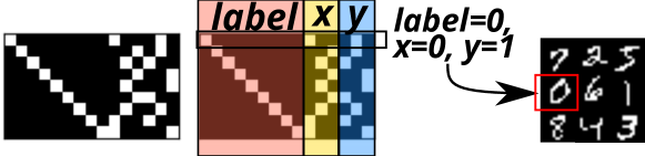
Figure 6: A single 8-puzzle state as a 9x15 matrix, representing 9 objects of 15 features. The first 9 features are the tile numbers and the other 6 features are the 1-hot x/y-coordinates.

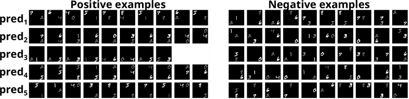
Figure 7: The positive/negative examples of the arguments for the first 5 predicates of $(U,A,P)=(25,2,50)$. The first/second argument is visualized in white / gray. We could interpret the condition for each $\textit{pred}_{p}$ returning true as follows: $\textit{pred}_{1}$: $(x_{1},y_{1})=(0,0)$ and $(x_{2},y_{2})=(*,1)$. $\textit{pred}_{2}$: $(x_{1},y_{1})=(2,1)$ and $(x_{2},y_{2})=(2,*)$. $\textit{pred}_{3}$: $y_{1}=y_{2}=2$ and $x_{1}<x_{2}$. $\textit{pred}_{4}$: $(x_{1},y_{1})=(2,*)$ and $(x_{2},y_{2})=(2,0)$. $\textit{pred}_{5}$: $(x_{1},y_{1})=(1,0)$ and $(x_{2},y_{2})=(2,*)$. $*$ denotes the wildcard.

Are Higher Arity Predicates Truly Necessary?

Previous work on relational structures has not yet provided evidence that they help to model the environment and extract abstract knowledge. For example, it is possible that even if a relational structure like RN (?) extracts multiple arguments, the succeeding layers may ignore some arguments by assigning zero weights, essentially modeling just unary predicates (i.e. attributes) rather than the structural relationships. We need to show direct evidence that the FOSAE extracts the essential higher-arity relations, without entangling the system with the policy learning structures.

One way to show that PNs are extracting higher-arity relations is to compare the minimum capacity required for the network to reconstruct the input for each arity $A$. The intuition here is that high-arity relations provide abstract knowledge that helps to compress the information. For example, with a (x-next ?o1 ?o2) relationship, the network does not have to encode the absolute information for every objects (e.g., (x0 o1) (y0 o1) (x1 o2) (y0 o2): 4bits) and rather the minimal amount of absolute information tied with a couple of relative information (e.g., (x0 o1) (y0 o1) (x-next o1 o2): 3bits). This is in line with the concepts in generic compression algorithms which try to minimize the redundant information. Note that we do not claim that the meaning of the predicates extracted by a PN is always such adjacency relations. In our unsupervised setting, we do not control (supervise) the type of relations the network decides to represent.

We made the contour plots (Fig. 8) of the reconstruction errors for the test set with various $U,P,A$, and compared their Pareto fronts. For the same $(U,P)$ pair, the size of the bottleneck layer (propositional vector) is $U\times P$ regardless of $A$, which makes the direct comparison between different $A$ feasible. We see that the arity plays a critical role in finding the more compact information, demonstrating that structural relations contribute to building an abstract representation.

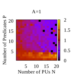
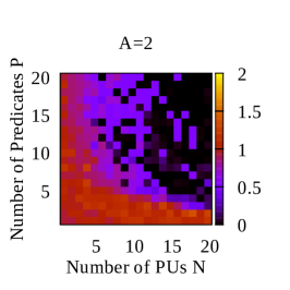
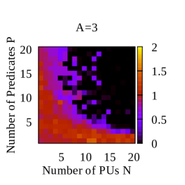
Figure 8: Contour plots of the reconstruction error of the test set for $A$=1,2,3, $(U,P)\in[1..20]^{2}$. It shows that the larger arity helps to learn the compact representation.

We also compared the number of trainable parameters (weights) in the network because, for the same $(U,P)$, the larger arity means the larger number of parameters in the networks which may help the training. Table 1 shows the models with the fewest parameters among those achieved the reconstruction error $\leq 0.1$ for each $A$. FOSAE with a larger arity can indeed be trained with fewer weights.

$A$	$U$	$P$	Propositions	Trainable parameters
1	18	5	90	287343
2	9	6	54	268273
3	9	7	63	303302
9	1	171	171	811828
SAE (Asai 2018)			18	3404467

Table 1: Configurations $(U,P)\in[1,20]^{2}$ for each $A$ that achieved the reconstruction error $\leq 0.1$ with the smallest trainable parameters. Arity $A$=2,3 achieved the human-indiscernible accuracy with a fewer number of parameters than $A$=1, while finding the smaller representations. This shows that the relational structures indeed help to model the environment by introducing a higher level of abstraction. Next, with $A$=9,$U$=1 tested over $P\in[1,400]$, the network is allowed to look at all objects and finds independent propositions while sharing the FOSAE architecture and other hyperparameters. It requires significantly larger parameters and latent representations. Finally, while the standard SAE (?) finds a more compressed representation, it consumes 10x more weight parameters.

We also compared the combination $(A,U)=(9,1)$ with $P\in[1..400]$, where 400 is the same maximum latent space capacity as the previous experiment. Since the predicates are allowed to see all objects ($A$=9), they are functions from the environment itself to a single boolean value, i.e. propositions, while maintaining the same FOSAE architecture. Table 1 shows that this configuration performs poorly, providing further evidence that the relations help obtain a compact, abstract representation.

We also confirmed that the standard SAE (?) consumes 10x more weight parameters even when tuned to have the minimal number of propositions under the reconstruction error $\leq 0.1$. This is because, in a fully propositional SAE, each proposition is independently learned even if some propositions are carrying similar information for the different objects. This is similar to what a convolutional layer is to a fully connected layer for image processing, where the former uses the shared filters to process the different local image patches.

Interpreting Predicates

Next, we show how the hard attentions make the predicates interpretable through visualization. In principle, we can visualize the objects in the images selected by the attentions (e.g., monkeys, bananas in Fig. 1) using a decoder function that reconstructs the regions from feature vectors. For the 8-puzzle feature vectors that we manually created for this experiment (Fig. 6), we instead use a hand-crafted decoder that pastes the corresponding image patch for the tile to the region specified by the xy-coordinates. Thanks to the hard, discrete attention activated by Gumbel-Softmax, no two objects are mixed.

Fig. 7 shows the visualizations of the arguments given to the predicate networks under hyperparameter $(U,A,P)=(25,2,50)$. Each subfigure is a visualization of an argument list vector ${\bm{g}}_{u}=({\bm{g}}_{u1},{\bm{g}}_{u2})$ randomly sampled from the dataset. Examples in the same row correspond to one predicate, where the left half represent the arguments which made the predicate true, and the right half represents those which made it false. We humans could recognize the patterns that are shared on the left-hand side of each row, giving us the possibility of interpretation which is not available in the fully propositional representation.

7 Evaluating Classical Planning Capability

We show that the FOL representation generated by FOSAE is a feasible and sound representation for classical planning.

We tested the FOSAE-generated representation with AMA₁ PDDL generator and the Fast Downward (?) classical planner. AMA₁ is an oracular method that takes the entire raw state transitions, encode each ${\left\{pre_{i},suc_{i}\right\}}$ pair with the SAE, then instantiate each encoded pair into a grounded action schema. It models the ground truth of the transition rules, thus is useful for verifying the state representation. Planning fails when SAE fails to encode a given init/goal image into a propositional state that exactly matches one of the search nodes. While there are several learning-based AMA methods that approximate AMA₁ (e.g., AMA₂ (?) and Action Learner (?)), there is information loss between the learned action model and the original search space generated by FOSAE, which make them unsuitable for our purpose of testing the feasibility of the representation.

AMA₁ is a fully propositional AMA method. To run AMA₁, we use the propositional output of PNs as the state representation, not the first-order representation. We leave the task of obtaining the lifted action model as future work.

We invoke Fast Downward with blind heuristics in order to remove the effect of the heuristics. This is primarily because AMA₁ generates a huge PDDL model containing every transition which results in an excessive runtime for initializing any sophisticated heuristics. The scalability issue caused by using a blind heuristics is not an issue since the focus of this evaluation is on the feasibility of the representation.

7.1 8 Puzzle

We generated 40 instances of 8-puzzle each generated by a random walk from the goal state. 40 instances consist of 20 instances each generated by a 7-steps random walk and another 20 by 14 steps. Results (Table 2) show that the planner successfully solves all problems, demonstrating that the representation grounded by the FOSAE is sound for planning.

random walk	#solved	search time [sec]	cost
steps	/ #total	(mean)	(mean)
8 Puzzle
7 steps	20/20	0.0014	7.00
14 steps	20/20	0.0236	13.60
3-blocks Blocksworld
3 steps	10/10	0.0013	2.2
7 steps	10/10	0.0062	3.6
14 steps	10/10	0.0226	5.7

Table 2: The number of instances solved by FOSAE + AMA₁ on the object vector based 8-puzzle instances and 3-blocks Blocksworld instances. The number of random walk steps counts the steps to generate a goal state from the initial state. The cost column in the 14 steps instances shows that it finds a solution shorter than 14, which is natural because the 14 steps random walk do not always correspond to the optimal solution of the puzzle.

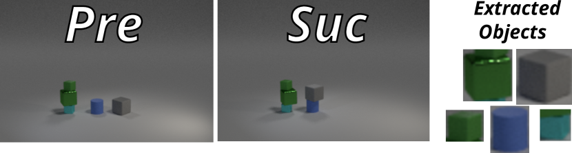
Figure 9: An example Blocksworld transition. Each state has a perturbation from the jitter in the light positions and the ray-tracing noise. Other objects may intrude the extracted regions. Objects have different sizes, colors, shapes (cube or cylinder) and surface materials (metal or rubber).

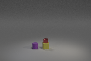
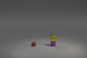
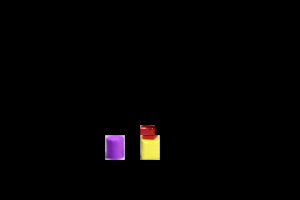
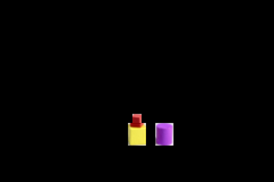
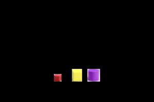
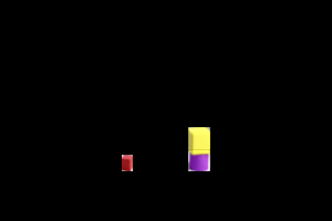
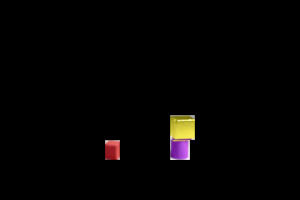
Figure 10: (middle) The initial/goal state of a Blocksworld instance. (right) The solution to this problem reconstructed from the latent vector. It unpolishes the red cube, then moves the cylinder, the red cube, the yellow cube and then polishes the yellow cube. The colors of blocks are affected by the preprocessing (histogram normalization) which helps the training.

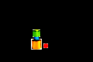
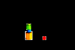
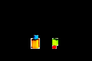
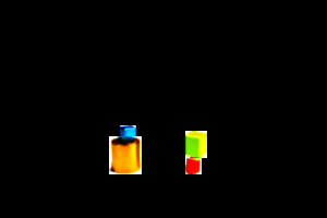
Figure 11: A successful plan execution for 4 blocks.

7.2 Photo-Realistic Blocksworld

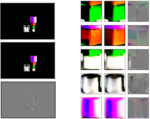
Figure 12: (left) The visualization of the autoencoding result using FOSAE in a 5 blocks, 3 stacks environment. The input (ground truth) is presented on the top, and the output (reconstruction) is presented in the middle. The bottom figure shows the difference between the input and the output. (right) The enlarged results of the reconstructions for the individual image patches. From the left, the ground truth, the reconstruction, and the pixel value difference.

In order to test the ability of the system in a more realistic environment, we prepared a photo-realistic Blocksworld dataset (Fig. 10) (?) which contains the blocks world states rendered by Blender 3D engine. There are several cylinders or cubes of various colors and sizes and two surface materials (Metal/Rubber) stacked on the floor, just like in the usual STRIPS Blocksworld domain. In this domain, three actions are performed: move a block onto another stack or on the floor, and polish/unpolish a block, i.e., change the surface of a block from Metal to Rubber or vice versa. All actions are applicable only when the block is on top of a stack or on the floor. The latter actions allow changes in the non-coordinate features of object vectors.

The dataset generator produces a 300x200 RGB image and a state description which contains the bounding boxes (bbox) of the objects. Extracting these bboxes is an object recognition task we do not address in this paper, and ideally, should be performed by a system like YOLO (?). We resized the extracted image patches in the bboxes to 32x32 RGB, flattened it into a 3072-D vector, and concatenated it with the bbox vector. The bbox vector is 200-dimensional and is generated by discretizing $(x_{1},y_{1},x_{2},y_{2})$ by 5 pixels and encoding it as a 1-hot vector (60/40 categories for each $x$/$y$-axis), resulting in 3072+200=3272 features per object. FOSAE encodes and reconstructs a set of feature vectors, each containing both the pixel and the bbox information. The feature vectors can be visualized by pasting the pixels into the bbox on a black canvas.

The generator enumerates all possible states/transitions (480/2592 for 3 blocks and 3 stacks; 5760/34560 for 4 blocks and 3 stacks; 80640/518400 for 5 blocks and 3 stacks). For training the FOSAE, we used 432 (90%, 3 blocks 3 stacks), 2500 (4 blocks 3 stacks), and 4500 states (5 blocks, 3 stacks), respectively. We chose $(U,A,P)=(10,2,100)$ as the hyperparameter. An example reconstruction is shown in Fig. 12.

We then solved 30 planning instances generated by taking a random initial state and choosing the goal states by the 3, 7, or 14 steps random walks (10 instances each). The system correctly solved all instances, where the correctness of the plan was checked manually. Fig. 10 shows an example solution generated from the intermediate states of the plan. We only performed planning for the 3 blocks environment due to the sheer size of the PDDL model generated by AMA₁ which contains 518400 actions and required more than 128GB memory to preprocess the model into a SAS+ format. We later performed some 4-blocks experiments and obtained success (Fig. 11).

8 Discussion and Conclusion

We proposed First-Order State AutoEncoder, a neural architecture which grounds/extracts first-order logical predicates from the environment without human supervision. Unlike any existing work to our knowledge, the training is fully automated (no manual tagging / no predefined reinforcement signals) and the resulting representation is interpretable, verifiable and compatible with symbolic systems such as classical planners.

We also provided the first empirical evidence that the relations between the objects help to model the environment by testing the architecture with various predicate arities. FOSAE exclusively models the environment, unlike a black-box mixture of the policy and the representation learned by Reinforcement Learning frameworks.

While the predicates grounded by the FOSAE are anonymous symbols that do not necessarily correspond to the human symbols (e.g., next), an interesting avenue of future work is to adapt the system to the semi-/supervised setting, where the supervised signals are fed into the latent layer (?). This could teach FOSAE the human symbols in the hand-coded knowledge base. Since semi-supervised/supervised learning are in general considered easier than unsupervised learning (done by our FOSAE), this is a promising direction.

Finally, note that we did not address the full FOL generalization, that is, the learned FOL statements are quantifier-free, grounded representation. Despite the limitation, this work is an important step toward the full FOL generalization – after all, to lift a FOL formula, the formula must be generated from the subsymbolic input in the first place. The next step is to lift the representation in order to extract action rules, axioms, and invariants, which enable the sophisticated heuristics developed in the heuristic search literature. Extending or leveraging the existing Action Model Acquisition methods (e.g., AMA₁, AMA₂, Action Learner (?), (?; ?; ?)) is an important avenue for future work.

References

- [Amado et al. 2018] Amado, L.; Pereira, R. F.; Aires, J.; Magnaguagno, M.; Granada, R.; and Meneguzzi, F. 2018. Goal Recognition in Latent Space. In Proceedings of the International Joint Conference on Neural Networks (IJCNN).
- [Asai and Fukunaga 2018] Asai, M., and Fukunaga, A. 2018. Classical Planning in Deep Latent Space: Bridging the Subsymbolic-Symbolic Boundary. In Proceedings of AAAI Conference on Artificial Intelligence.
- [Asai 2018] Asai, M. 2018. Photo-realistic blocksworld dataset. arXiv:1812.01818.
- [Bahdanau, Cho, and Bengio 2015] Bahdanau, D.; Cho, K.; and Bengio, Y. 2015. Neural Machine Translation by Jointly Learning to Align and Translate. In Proceedings of the International Conference on Learning Representations.
- [Battaglia et al. 2018] Battaglia, P. W.; Hamrick, J. B.; Bapst, V.; Sanchez-Gonzalez, A.; Zambaldi, V.; Malinowski, M.; Tacchetti, A.; Raposo, D.; Santoro, A.; Faulkner, R.; et al. 2018. Relational inductive biases, deep learning, and graph networks. arXiv:1806.01261.
- [Cresswell, McCluskey, and West 2013] Cresswell, S.; McCluskey, T. L.; and West, M. M. 2013. Acquiring planning domain models using LOCM. Knowledge Eng. Review 28(2):195–213.
- [Garnelo, Arulkumaran, and Shanahan 2016] Garnelo, M.; Arulkumaran, K.; and Shanahan, M. 2016. Towards Deep Symbolic Reinforcement Learning. arXiv preprint arXiv:1609.05518.
- [Graves et al. 2016] Graves, A.; Wayne, G.; Reynolds, M.; Harley, T.; Danihelka, I.; Grabska-Barwińska, A.; Colmenarejo, S. G.; Grefenstette, E.; Ramalho, T.; Agapiou, J.; et al. 2016. Hybrid Computing using a Neural Network with Dynamic External Memory. Nature 538(7626):471–476.
- [Gumbel and Lieblein 1954] Gumbel, E. J., and Lieblein, J. 1954. Statistical theory of extreme values and some practical applications: A series of lectures.
- [Harnad 1990] Harnad, S. 1990. The symbol grounding problem. Physica D: Nonlinear Phenomena 42(1-3):335–346.
- [Helmert 2004] Helmert, M. 2004. A Planning Heuristic Based on Causal Graph Analysis. In Proceedings of the International Conference on Automated Planning and Scheduling(ICAPS), 161–170.
- [Hoffmann and Nebel 2001] Hoffmann, J., and Nebel, B. 2001. The FF Planning System: Fast Plan Generation through Heuristic Search. J. Artif. Intell. Res.(JAIR) 14:253–302.
- [Jang, Gu, and Poole 2017] Jang, E.; Gu, S.; and Poole, B. 2017. Categorical Reparameterization with Gumbel-Softmax. In Proceedings of the International Conference on Learning Representations.
- [Kingma and Ba 2015] Kingma, D., and Ba, J. 2015. Adam: A Method for Stochastic Optimization. In Proceedings of the International Conference on Learning Representations.
- [Kingma et al. 2014] Kingma, D. P.; Mohamed, S.; Rezende, D. J.; and Welling, M. 2014. Semi-Supervised Learning with Deep Generative Models. In Advances in Neural Information Processing Systems, 3581–3589.
- [LeCun, Bengio, and Hinton 2015] LeCun, Y.; Bengio, Y.; and Hinton, G. 2015. Deep Learning. Nature 521(7553):436.
- [Maddison, Tarlow, and Minka 2014] Maddison, C. J.; Tarlow, D.; and Minka, T. 2014. A* sampling. In Advances in Neural Information Processing Systems, 3086–3094.
- [Manhaeve et al. 2018] Manhaeve, R.; Dumančić, S.; Kimmig, A.; Demeester, T.; and De Raedt, L. 2018. DeepProbLog: Neural Probabilistic Logic Programming. In Advances in Neural Information Processing Systems.
- [McDermott 2000] McDermott, D. V. 2000. The 1998 AI Planning Systems Competition. AI Magazine 21(2):35–55.
- [Mnih et al. 2015] Mnih, V.; Kavukcuoglu, K.; Silver, D.; Rusu, A. A.; Veness, J.; Bellemare, M. G.; Graves, A.; Riedmiller, M.; Fidjeland, A. K.; Ostrovski, G.; et al. 2015. Human-Level Control through Deep Reinforcement Learning. Nature 518(7540):529–533.
- [Mnih, Heess, and Graves 2014] Mnih, V.; Heess, N.; and Graves, A. 2014. Recurrent models of visual attention. In Advances in Neural Information Processing Systems, 2204–2212.
- [Mohit 2014] Mohit, B. 2014. Named Entity Recognition. In Natural language processing of semitic languages. Springer. 221–245.
- [Mourão et al. 2012] Mourão, K.; Zettlemoyer, L. S.; Petrick, R. P. A.; and Steedman, M. 2012. Learning STRIPS Operators from Noisy and Incomplete Observations. In Proceedings of the International Conference on Uncertainty in Artificial Intelligence, 614–623.
- [Nadeau and Sekine 2007] Nadeau, D., and Sekine, S. 2007. A Survey of Named Entity Recognition and Classification. Lingvisticae Investigationes 30(1):3–26.
- [Paccanaro and Hinton 2001] Paccanaro, A., and Hinton, G. E. 2001. Learning Distributed Representations of Concepts using Linear Relational Embedding. IEEE Transactions on Knowledge and Data Engineering 13(2):232–244.
- [Redmon et al. 2016] Redmon, J.; Divvala, S.; Girshick, R.; and Farhadi, A. 2016. You Only Look Once: Unified, Real-Time Object Detection. In Proceedings of IEEE Conference on Computer Vision and Pattern Recognition, 779–788.
- [Rocktäschel and Riedel 2017] Rocktäschel, T., and Riedel, S. 2017. End-to-end Differentiable Proving. In Guyon, I.; Luxburg, U. V.; Bengio, S.; Wallach, H.; Fergus, R.; Vishwanathan, S.; and Garnett, R., eds., Advances in Neural Information Processing Systems. Curran Associates, Inc. 3788–3800.
- [Russell et al. 1995] Russell, S. J.; Norvig, P.; Canny, J. F.; Malik, J. M.; and Edwards, D. D. 1995. Artificial Intelligence: A Modern Approach, volume 2. Prentice hall Englewood Cliffs.
- [Santoro et al. 2017] Santoro, A.; Raposo, D.; Barrett, D. G.; Malinowski, M.; Pascanu, R.; Battaglia, P.; and Lillicrap, T. 2017. A simple neural network module for relational reasoning. In Advances in Neural Information Processing Systems, 4967–4976.
- [Scarselli et al. 2009] Scarselli, F.; Gori, M.; Tsoi, A. C.; Hagenbuchner, M.; and Monfardini, G. 2009. The Graph Neural Network Model. IEEE Transactions on Neural Networks 20(1):61–80.
- [Sourek et al. 2018] Sourek, G.; Aschenbrenner, V.; Zelezny, F.; Schockaert, S.; and Kuzelka, O. 2018. Lifted Relational Neural Networks: Efficient Learning of Latent Relational Structures. J. Artif. Intell. Res.(JAIR) 62:69–100.
- [Steels 2008] Steels, L. 2008. The Symbol Grounding Problem has been Solved. So What’s Next? In de Vega, M.; Glenberg, A.; and Graesser, A., eds., Symbols and Embodiment. Oxford University Press.
- [Taddeo and Floridi 2005] Taddeo, M., and Floridi, L. 2005. Solving the Symbol Grounding Problem: A Critical Review of Fifteen Years of Research. Journal of Experimental & Theoretical Artificial Intelligence 17(4):419–445.
- [van Steenkiste et al. 2018] van Steenkiste, S.; Chang, M.; Greff, K.; and Schmidhuber, J. 2018. Relational Neural Expectation Maximization: Unsupervised Discovery of Objects and their Interactions. In Proceedings of the International Conference on Learning Representations.
- [Xu et al. 2015] Xu, K.; Ba, J.; Kiros, R.; Cho, K.; Courville, A.; Salakhudinov, R.; Zemel, R.; and Bengio, Y. 2015. Show, attend and tell: Neural image caption generation with visual attention. In Proceedings of the International Conference on Machine Learning, 2048–2057.
- [Yang, Wu, and Jiang 2007] Yang, Q.; Wu, K.; and Jiang, Y. 2007. Learning Action Models from Plan Examples using Weighted MAX-SAT. Artificial Intelligence 171(2-3):107–143.
- [Zambaldi et al. 2018] Zambaldi, V.; Raposo, D.; Santoro, A.; Bapst, V.; Li, Y.; Babuschkin, I.; Tuyls, K.; Reichert, D.; Lillicrap, T.; Lockhart, E.; et al. 2018. Relational Deep Reinforcement Learning. arXiv:1806.01830.