TREVR: A general $N\log^{2}N$ radiative transfer algorithm

Abstract

We present TREVR (Tree-based REVerse Ray Tracing), a general algorithm for computing the radiation field, including absorption, in astrophysical simulations. TREVR is designed to handle large numbers of sources and absorbers; it is based on a tree data structure and is thus suited to codes that use trees for their gravity or hydrodynamics solvers (e.g. Adaptive Mesh Refinement). It achieves computational speed while maintaining a specified accuracy via controlled lowering of the resolution of both sources and rays from each source. TREVR computes the radiation field in order ${N\log N_{\rm source}}$ time without absorption and order ${N\log N_{\rm source}\log{N}}$ time with absorption. These scalings arise from merging sources of radiation according to an opening angle criterion and walking the tree structure to trace a ray to a depth that gives the chosen accuracy for absorption. The absorption-depth refinement criterion is unique to TREVR. We provide a suite of tests demonstrating the algorithm’s ability to accurately compute fluxes, ionization fronts and shadows.

1 Introduction

Radiation, arguably, plays the determining role in the field of astrophysics. Almost all of the information we receive from the cosmos comes in the form of photons we detect on or around earth. Understanding the process of radiative transfer (RT) is required to interpret this information, as the photons are affected by the media they travel through on their way to our telescopes and detectors. Interactions between photons and these media not only affect the photons themselves but the matter as well. Photons and baryons exchange energy and momentum, driving both heating and cooling. This also affects excitation and ionization states and thus determines the chemical and thermodynamic properties of the gas. Thus radiation is a key player in many of the astrophysical systems and processes we study.

On galaxy scales, a central question is how feedback mechanisms affect star and galaxy formation. Stellar feedback comes in the form of photoionization by ultraviolet (UV) radiation, stellar winds and supernovae (e.g. Leitherer et al., 1999), the latter of which has been a main focus in simulations in previous years (e.g. Agertz et al., 2013). It is important to note that even though supernovae might be spectacularly powerful events, ionizing radiative output from stellar populations contributes two orders of magnitude more energy at early times and about 50 times more energy over the course of a stellar population’s lifetime. This is evident from Figure 1, which is a plot of the luminous output per solar mass as a function of time from a typical stellar population (computed using the stellar evolution code Starburst99; Leitherer et al. 1999).

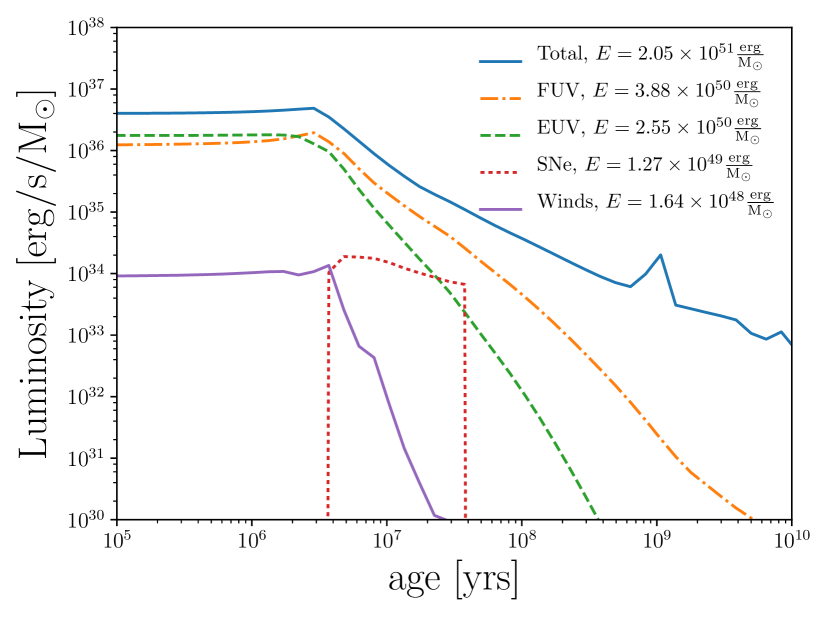
Figure 1: Luminosity per solar mass as a function of time for a stellar population having a Chabrier initial mass function (Chabrier, 2003).

However, the way in which this massive output of UV radiation is deposited and consequently affects the interstellar medium (ISM) is still unclear. Attempts at numerically exploring these effects without the use of a full radiative transfer method have produced conflicting results. Simulations done by Gritschneder et al. (2009) and Walch et al. (2012) suggest that ionizing feed back from large O-type stars before the first supernovae ($\sim 1-3\ \rm{Myr}$) have a significant effect on star formation rate. Whereas Dale et al. (2012) conclude the effect on the star formation rate to be small.

With this potential impact in mind, it may seem surprising that RT has been treated poorly in most galaxy-scale astrophysical simulations, often as an imposed uniform background. This is because RT is an intrinsically complex and computationally expensive problem. The complexity is immediately evident from the full RT equation (e.g. Mihalas & Mihalas, 1984),

$$\left[\frac{1}{c}\frac{\partial}{\partial t}+\mathbf{n\cdot\nabla}\right]I\left(\mathbf{x},\mathbf{n},t,\nu\right)=$$

$$\epsilon\left(\mathbf{x},\mathbf{n},t,\nu\right)-\alpha\left(\mathbf{x},\mathbf{n},t,\nu\right)I\left(\mathbf{x},\mathbf{n},t,\nu\right).$$ (1)

Here, $I$, $\epsilon$ and $\alpha$ are the intensity, emissivity and extinction coefficients respectively and all depend on position $\mathbf{x}$, unit direction of light propagation $\mathbf{n}$, time $t$ and frequency $\nu$. Apart from being a seven dimensional problem, RT involves the highest possible characteristic speed, $c$, the speed of light. Also, unlike a similar problem such as gravity, RT depends on the properties of the intervening material via the absorption term, $\alpha$.

Because of this complexity, a naïve numerical solution to the RT problem scales with the number of resolution elements, $N$, as $\mathcal{O}\left(N^{7/3}\right)$ and requires a timestep thousands of times smaller than typical Courant times in astrophysics. This scaling arises due to three contributions. Firstly, a radiation field must be computed at each of the simulation’s $N$ resolution elements. Secondly, each one of the resolution element’s intensity values is made up of contributions from $N_{\rm source}$ sources of radiation ($N_{\rm source}$ rays of light being computed per resolution element). This leads to a scaling for the total number of rays of $N_{\rm ray}=N\times N_{\rm source}$, or $\mathcal{O}\left(N^{2}\right)$ assuming that $N_{\rm source}\sim N$. This fact alone limits brute-force RT methods to only small-scale problems, such as ionization by a few massive stars (e.g. Howard et al., 2016, 2017). Finally, each ray of light interacts with the medium along its path, which is resolved with $\mathcal{O}\left(N^{1/3}\right)$ resolution elements. Thus the computational cost is $\mathcal{O}\left(N^{7/3}\right)$. This poor scaling with number of resolution elements makes it infeasible, or at least unattractive, to simulate RT alongside gravity and hydrodynamics methods that scale as $\mathcal{O}\left(N\log N\right)$ or better. It is evident that much can be gained by reducing the linear dependence on $N_{\rm source}$, with additional gains from tackling the $N^{1/3}$ cost per ray.

A practicable RT method would have to solve a simplified RT problem. RT methods can be divided into two different categories based on how they treat $c$ in Equation 1.

Evolutionary methods use a finite $c$, (which is often reduced from the true speed of light) and thus the partial time derivative remains in Equation 1, and the radiation field is advected or evolved thoughout the simulation. The prototypical evolutionary method is flux-limited diffusion (FLD) (Levermore & Pomraning, 1981). Modern evolutionary methods include moment methods like OTVET (Gnedin & Abel, 2001) and RAMSES-RT (Rosdahl et al., 2013) as well as photon packet propagation methods like TRAPHIC (Pawlik & Schaye, 2008), SPHRAY (Altay et al., 2008) and SimpleX2 (Paardekooper et al., 2010).

Instantaneous methods, on the other hand, take the limit where $c$ is infinite and the partial time derivative in Equation 1 goes to zero. In this case the radiation field can be computed instantaneously as a geometric problem. Computational methods in this category include forward raytracers such as $\rm C^{2}Ray$ (Mellema et al., 2006), Moray (Wise & Abel, 2011) and Fervent (Baczynski et al., 2015) as well as reverse raytracers such as TreeCol (Clark et al., 2012), URCHIN (Altay & Theuns, 2013) and TREERAY (Wünsch et al., 2018; Haid et al., 2018).

Instantaneous methods typically take the form of raytracers. Raytracers are the most direct way to solve the RT problem. Forward raytracers trace many rays outward from sources of radiation, similarly to the actual phenomenon, in the hope that resolution elements will have sufficiently many rays intersecting them to compute a radiation field. Naïvely, the number of rays per source would be comparable to the number of resolution elements, giving a scaling of $\mathcal{O}\left(NN_{\rm source}N^{1/3}\right)$, as previously noted. However, for forward ray tracing, $\mathcal{O}\left(N^{2/3}\right)$ rays per source are typically sufficient to hit every resolution element when extended to the edge of the simulation volume (distance $\mathcal{O}\left(N^{1/3}\right)$), so the scaling typically achieved is $\mathcal{O}\left(NN_{\rm source}\right)$.

It is important to note when methods adaptively split rays (e.g. using Healpix Górski et al. 2005 as in Moray, URCHIN and TreeCol), it does not change the overall scaling. For example, a centrally located source requires $6\,N^{2/3}$ rays to strike all elements in the outer faces of a cubical simulation volume, each with a length $\mathcal{O}\left(N^{1/3}\right)$. Even with adaptive ray merging near the source, at least $N$ ray segments are required to intersect each of the $N$ resolution elements. In addition, raytracers such as Moray rely upon a Monte-Carlo approach to estimate the radiation field and thus require at least 10 rays to intersect each element, a constant but significant prefactor to the overall cost. This scaling usually limits forward raytracers to problems with few sources to avoid $\mathcal{O}(N^{2})$-like scaling.

Recently there has been some focus on reverse ray tracing methods by Clark et al. (2012), Altay & Theuns (2013), Woods (2015) (applied in Kannan et al. 2014) and Haid et al. (2018). The first two methods listed are not general, as they are designed to compute external radiation (e.g. from the post-ionization UV background) rather than internal sources of radiation. The latter two methods are more general and can handle internal sources.

The idea of reverse ray tracing introduces some advantages relative to forward ray tracing. Reverse raytracers trace all the rays that strike a specific resolution element before moving to the next element. Algorithmically, this is equivalent to tracing in reverse, from the sinks to the sources. This makes it easy to ensure that the source and absorber angular distributions are well-sampled near the resolution element as opposed to forward ray tracing where one would have to increase the number of rays per source to guarantee this type of accuracy. Put simply, radiation is computed exactly where it is needed. This is especially advantageous in adaptive mesh and Lagrangian simulations such as smoothed particle hydrodynamics (SPH), as low density regions are represented by few resolution elements, and thus extra work is not done to resolve radiation in those regions.

A key benefit to reverse ray tracing is the potential for adaptive timesteps to dramatically reduce the radiation work as only active resolution elements, $N_{\rm sink}$, need to be traced to. This active subset can be a million times smaller than $N$ in, for example, high-resolution cosmological simulations. Typical hydro and gravity codes achieve a factor of 100 speed-up by taking advantage of this so it is important that the radiation code has the same capability or radiation will overwhelm the computation. Thus a naïve reverse ray trace still scales as $\mathcal{O}\left(N_{\rm sink}N_{\rm source}N^{1/3}\right)$, with the presence of many sources presenting the most significant computational barrier.

In contrast, evolutionary methods are typically based on evolving moments of the radiation field stored at each resolution element. They are insensitive to the number of sources, and scale as $\mathcal{O}(N)$ with the number of resolution elements, allowing them to handle large numbers of sources and scattering. Although evolutionary methods can handle both optically thin and thick regimes, they lose directional accuracy in intermediate regimes and suffer from poor directional accuracy in general. This is immediately apparent in shadowing tests (e.g. Figure 16 in Rosdahl et al. 2013).

Photon packet propagation methods, such as TRAPHIC (Pawlik & Schaye, 2008), employ an evolutionary approach in which directional accuracy is easier to control, in principle. However, the Monte-Carlo aspects of how photon packets are propagated introduce significant Poisson noise into their computed radiation field. Added Monte-Carlo re-sampling is shown to reduce this noise but it is quite expensive and degrades the initially sharp shadows. For this reason it is typically not used in production runs. TRAPHIC also adds virtual particles (ViPs) to propagate their photon packets in less dense, optically thin regions lacking in SPH particles. TRAPHIC scales linearly with resolution elements, as mentioned before, multiplied by the number of packets per element (typically 32-64).

A key limitation for evolutionary methods, whether they are moment or packet-tracing methods, is that the radiation field for every element needs to be computed every timestep. In addition, the speed of light, even when reduced, is substantially larger than the sound speed and thus many radiation substeps are required compared to the hydro solver. Thus for photon packet propagation methods every photon packet typically hops forward several times for each hydro step even if most elements are not active. A key outcome is that moment methods cannot take advantage of adaptive timesteps to limit radiation work. Another issue, specific to TRAPHIC, is that $N$ is significantly greater than the number of SPH particles due to the addition of ViPs. These factors dramatically increase the prefactor on the scaling. Nonetheless, methods such as TRAPHIC represent an effective approach for large simulations that can handle a variety of regimes of optical depth.

Until now the poor scaling with source number, as $\mathcal{O}\left(N_{\rm source}N\right)$, has severely limited the applicability and competitiveness of instantaneous ray tracing relative to evolutionary methods such as TRAPHIC. Recently however, Woods (2015) and Wünsch et al. (2018) developed promising generalizations of reverse ray tracing based on merging of sources that can handle large numbers of internal sources. The basic idea is to use a tree to combine distant sources and reduce the cost to $\mathcal{O}\left(N\log N\right)$. Wünsch et al. (2018) implemented the TREERAY reverse raytracer in the FLASH AMR code (Fryxell et al., 2000). They employ an Oct-tree, a fixed number of rays (48) per source and calculate absorption on the fly during the tree-walk. The primary weakness of the Woods (2015) and Wünsch et al. (2018) methods is that they lower the resolution along rays in a preset manner. This prevents them from maintaining the accuracy of the received flux at higher optical depths. Doing so requires multiple adaptivity criteria. This means going beyond the open angle used in tree codes. This is the focus of the current work.

In this paper we present TREVR (Tree-based Reverse Ray Tracing), an $\mathcal{O}\left(N\log^{2}N\right)$ adaptive reverse raytracer. In Section 2 we detail the specific RT equations TREVR solves (Subsection 2.1) and the general TREVR algorithm (Subsection 2.2) including its adaptivity criteria. TREVR is not specific to any one kind of code (e.g. Adaptive Mesh Refinement (AMR) vs. SPH). Here we provide details of our implementation in the Gasoline SPH code (Subsection 2.3). TREVR was developed from the method of Woods (2015) which was also implemented in Gasoline. In Section 3 we present a suite of tests demonstrating the algorithm’s ability to accurately compute fluxes, ionization fronts and shadows in the optically thick and thin regimes. These tests also allow us to explore how TREVR’s adaptivity criteria control error and affects computational cost. The computational cost is bounded and characterized in the general case to substantiate the $\mathcal{O}\left(N\log^{2}N\right)$ claim made earlier. Finally, in Section 4 we discuss TREVR’s strengths and shortcomings and conclude how they enable and constrain the types of problems TREVR can handle, and discuss improvements that can be made in the future.

2 Method

2.1 Simplifications to the full RT problem

Before describing TREVR, we will first define the simplified version of the classical RT equation that the method solves. Since TREVR is an instantaneous method, $c$ is set to infinity eliminating the partial time derivative in Equation 1 leaving us with the instantaneous RT equation:

$$\mathbf{n\cdot\nabla}I\left(\mathbf{x},\mathbf{n},t,\nu\right)=\epsilon\left(\mathbf{x},\mathbf{n},t,\nu\right)-\alpha\left(\mathbf{x},\mathbf{n},t,\nu\right)I\left(\mathbf{x},\mathbf{n},t,\nu\right).$$ (2)

The emissivity term in the above equation, $\epsilon$, describes a continuous emitting medium. TREVR could assume sources of radiation were continuous, but being a numerical method it needs to represent sources of radiation as discrete resolution elements such as “star particles”. In this case $\epsilon$ is a sum of delta functions and the solution to the RT equation becomes a linear combination of contributions from all sources of radiation. Also, since we are considering sources one by one we can start using the path length $s$ between a source and resolution element as our integration element and examine just one direction, $\mathbf{n}$,

$$\frac{dI}{ds}=-\alpha I.$$ (3)

We can then combine the path length and extinction coefficient to solve for intensity by integrating

$$d\tau=\alpha ds=\kappa\rho ds,$$ (4)

for $\tau$, the optical depth, where $\kappa$ is opacity and $\rho$ is density. This leads to

$$\frac{dI}{d\tau}=-I,$$ (5)

which is the final version of the RT problem solved by this method. The solution to the equation is

$$I(s)=I(0)e^{-\tau(s)},$$ (6)

where $I(0)$ is the intensity of the source and $\tau(s)$ is the quantity to be estimated in our method:

$$\tau(s)=\int_{0}^{s}\kappa(s)\rho(s)ds.$$ (7)

If we assume that the source of radiation is point-like, then the intensity at the receiver (the sink) is a delta function in angle. In this case, there is a one-to-one correspondence between the intensity and flux contributions due to that source. The flux is given by

$$\mathbf{F}=\int I(\Omega)\mathbf{n^{\prime}}(\Omega)d\Omega=I(s)\mathbf{n},$$ (8)

where $\mathbf{n}$ is the unit vector in the direction from the source to the sink.

For each source, $i$, we have a luminosity, $L_{i}$, which can be directly converted to a contribution to the flux at the sink,

$$\mathbf{F_{i}}=\frac{L_{i}}{4\pi s_{i}^{2}}e^{-\tau_{i}}\mathbf{n_{i}},$$ (9)

where $\tau_{i}$ is the accumulated optical depth along the ray between that source and the sink and $s_{i}$ is the distance. The net flux, $\mathbf{F}$, is then computed by summing up flux contributions from all sources.

The intensity due to a single source is,

$$I_{i}=\frac{L_{i}}{4\pi s_{i}^{2}}e^{-\tau_{i}}.$$ (10)

By summing the intensity from all sources we can get the angle-averaged intensity. We can use this averaged intensity directly in heating, chemistry and ionization rate expressions. For many applications in astrophysics this is the primary effect of the radiation field on local gas. We note that it is important to apply timestep limits to correctly follow the progress of ionization fronts as they change the absorption properties of the gas. This approach relies on the ionization front speed as the rate limiting step, rather than the speed of light.

The first order moment of the intensity is the net radiation flux. Higher order moments such as the radiation pressure, $\mathbf{p}$, can be easily obtained with simple summations.

2.2 Algorithm

The TREVR algorithm is based around a tree data structure which partitions the simulation volume hierarchically in space. The smallest resolution elements are, or are contained in the leaf nodes of the tree data structure. In Lagrangian or “particle” methods such as SPH, a number of SPH particles can be contained in a leaf node or “bucket”. The maximum number of particles per bucket is referred to as $N_{B}$. In Eulerian or “grid”-based methods the bucket is the smallest grid cell itself, so $N_{B}$ is effectively one. $N$ resolution elements hold radiation intensity values and represent the radiation field TREVR computes.

Note that although TREVR has been initially implemented in the SPH code Gasoline (Wadsley et al., 2017), TREVR is not specific to SPH. The method only requires that the simulation volume be hierarchically partitioned in space and so it could be used directly in an adaptive mesh refinement code. In the case of grid codes, the algorithm is simplified as the final SPH particle ray tracing step is not needed.

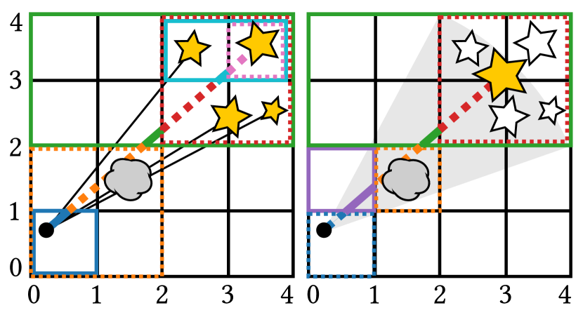
Figure 2: A schematic of TREVR without (left) and with source merging and adaptive refinement (right). Coloured ray segments correspond to tree cells whose average properties are used to compute the optical depth along that ray segment. Dashed and solid lines distinguish consecutive line segments to help associate them with their corresponding tree cell. The grey cloud represents a feature in the medium that requires refinement in order to be resolved. The smaller stars which are yellow in the left panel and white in the right panel represent individual radiation sources. The larger yellow star in the right panel represents a merged source, as the dashed red cell encapsulating all sources meets the opening angle (grey region in right panel) criterion.

2.2.1 Source Merging

As mentioned in the introduction, a naïve algorithm would compute interactions between a resolution element and all sources of radiation. If we assume the number of resolution elements is equal to the number of sources, an infeasible number of interactions would need to be computed, with scaling $\mathcal{O}\left(N^{2}\right)$. To mitigate this $N^{2}$ scaling TREVR employs source merging similar to particle merging in the Barnes & Hut (1986) tree-based gravity solver which has remained popular in astrophysics (Benz, 1988; Vine & Sigurdsson, 1998; Springel et al., 2001; Wadsley et al., 2004; Hubber et al., 2011). We first applied radiation source merging in a rudimentary version of TREVR that did not consider extinction of any kind (Kannan et al., 2014).

For a given sink point, sources of radiation inside a tree cell are merged together at their centre of luminosity if they meet an “opening angle” criterion. This criterion is defined as

$$\theta_{\rm open}>l/r,$$ (11)

where $l$ is the distance from the centre of luminosity to the furthest part of the tree cell, $r$ is distance from the sink to the closest cell edge and $\theta_{\rm open}$ is the opening angle, a fixed accuracy parameter. This is equivalent to the criterion used for gravity in Wadsley et al. (2004) and ensures parent cells of a point are always opened. Source merging considerably reduces the number of interactions TREVR computes. This is illustrated in the left panel of Figure 2, where the grey angle represents a cell whose angular size meets the opening angle criterion.

The cost savings of source merging can be quantified by integrating the number of tree cells that pass the opening angle criterion and whose contents are treated as a single source. We will call the total count of the cells used $N_{\rm cell}$. We can estimate $N_{\rm cell}$ by integrating spherical shells of thickness $dr$ along the path from a resolution element $r$, and then dividing the sphere volume by the volume of the cell, $V_{\rm cell}(r)$.

$$N_{\rm cell}=\int_{R_{B}}^{R}\frac{4\pi r^{2}}{V_{\rm cell}(r)}dr$$ (12)

The bounds of the integral are $R_{B}$, the size of a bucket cell, and $R$, the length of the simulation volume. Because the number of particles in a simulation is proportional to the simulation volume, the lower integration limit can be expressed using particle numbers via,

$$\frac{R_{B}}{R}=\left(\frac{N_{B}}{N}\right)^{1/3},$$ (13)

the cube root of the ratio of the average number of particles per bucket, $N_{B}$, to the total number of simulation particles. Again, note that $N_{B}$ is only needed for particle methods and is one otherwise. The cell volume can also be rewritten by cubing the opening angle parameter

$$V_{\rm cell}(r)=l^{3}=\theta_{\rm open}^{3}r^{3}.$$ (14)

Substituting gives us the following integral and its solution,

$$N_{\rm cell}=\int_{(N_{B}/N)^{1/3}}^{R}\frac{4\pi}{\theta_{\rm open}^{3}\,r}dr\sim\log{N/N_{B}}.$$ (15)

This result means that the number of interactions scales like $\mathcal{O}\left(N_{\rm sink}\log N\right)$. This is also the total cost scaling in the optically thin regime, as expected given that the RT problem is almost identical to the gravity problem in the absence of intervening material.

We next consider ray tracing in the optically thick regime.

2.2.2 Tracing Rays

In the presence of absorbing material along a ray, the optical depth needs to be computed following Equation 7. To solve this integral numerically, we traverse the tree between the source and resolution element to sum the optical depth. This requires that the tree partitions and fills space, thus all the intervening material is contained in the tree we traverse. Making use of properties computed during the tree build, we can compute the optical depth of the $i$-th piece of the ray, $\tau_{i}$, using the intersection length of the cell and ray, $s_{i}$, as well as the average density, $\bar{\rho}_{i}$, and average opacity, $\bar{\kappa}_{i}$, in the cell

$$\tau_{i}=\bar{\rho}_{i}\bar{\kappa}_{i}s_{i}.$$ (16)

The total optical depth is then summed up during the tree walk,

$$\tau=\sum_{i}\tau_{i},$$ (17)

giving us everything needed to evaluate Equation 9.

This process is illustrated in the left panel of Figure 2. In this figure ray segments and corresponding cells share the same colour. When referring to specific cell colours, they will also be identified by two sets of points, in the form $[(x,y),(x,y)]$, corresponding to the bottom left and top right vertices of the cell respectively. Dotted lines are used to distinguish consecutive ray segments and help associate ray segments with their corresponding cells. In the left panel of Figure 2 there are two important things to note. First, since we are performing a reverse ray trace, the resolution element denoted by the black circle is intrinsically well resolved at the bucket cell (the blue cell at $[(0,0),(1,1)]$) level. However, the second point is that as the tree is walked upwards, space becomes less resolved. It should be apparent that the central parts of the ray are less resolved (the green cell at $[(0,2),(4,4)]$) and as one moves towards the source or resolution element the ray becomes more resolved (the red cell at $[(2,2),(4,4)]$ and the orange cell $[(0,0),(2,2)]$). This can be considered in two ways. If the medium is uniform, the algorithm can be extremely efficient while still being able to resolve a sharp feature in the radiation field such as an ionization front. However, if the medium is highly irregular along the ray the algorithm will not be able to resolve sharp density and opacity gradients which could significantly alter the optical depth. Thus adaptive refinement is needed during the tree walk to accurately calculate the optical depth along the ray.

2.2.3 Adaptive Refinement

For each ray, TREVR decides whether to use the full resolution available or if a set of longer ray segments intersecting lower resolution parent cells would be sufficient. In principle, the resolution elements themselves could be subdivided based on properties associated with RT for even higher resolution, but that is beyond the scope of the present work.

Consider the right panel in Figure 2. A dense blob of gas to be resolved resides in the orange highlighted cell at $[(1,1),(2,2)]$. At the point in the tree walk where we reach the orange highlighted cell at $[(0,0),(2,2)]$ in the left panel, a decision needs to be made on whether the current cell sufficiently represents the medium. This decision is based on a refinement criterion. If the cell passes the criterion to refine, rather than using its average properties, we recursively check the cell’s children until the criterion fails. This process ensures we compute a better resolved section of the ray.

Difficulty comes in choosing a refinement criterion that is both accurate and efficient. Ideally, refinement occurs when the average optical depth in a region may not accurately reflect the true distribution, such as a clumpy medium where the average density and opacity is much higher than the “effective” density and opacity (Városi & Dwek, 1999; Hegmann & Kegel, 2003). For this reason, we developed a new, optical depth-based refinement criterion for TREVR.

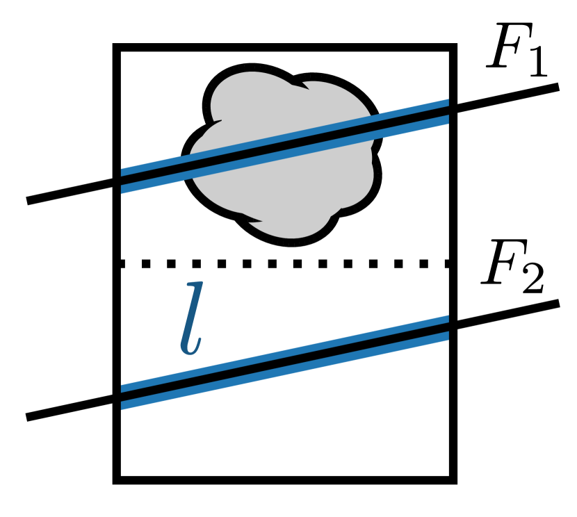
Figure 3: Schematic of a cell to be refined. A parent cell intersected by a ray contains a feature (grey cloud) to be resolved. The black dotted line partitions the parent cell into it’s children. The black intersecting rays represent the hypothetical case where only a child cell is intersected by a ray. The blue outlined sections on each ray correspond to the intersection length, $l$, used to compute the optical depth through each child cell.

Our criterion requires minimum and maximum absorption coefficients, $\alpha_{\rm min}$ and $\alpha_{\rm max}$, for each cell. These are estimated for the three Cartesian directions ($x,y,z$) separately. Leaf cells are assumed to have a single value $\alpha=\kappa\rho$. Then, for example, we estimate the minimum, $x$-direction optical depth of the parent cell via the minimum $x$-direction optical depths of the child cells. This requires taking the minimum for cases where the ray would intersect one child cell or the other or a sum for cases where the ray passes through both child cells. With axis-aligned cells and using Cartesian ray directions we know which case applies. We then divide by the new total $x$-cell width to recover an $\alpha_{\rm min}$ in the $x$-direction for the parent cell. The use of maxima and minima effectively takes into account diagonal rays with similar directions to the Cartesian direction (albeit in a conservative fashion because it assumes that two straight rays corresponding to minimal and maximal optical depth values always actually exist).

Proceeding in a bottom-up fashion during the tree build, we estimate directional minima and maxima $\alpha$ values for all cells. We then take the minima and maxima over the three directions and save just one $\alpha_{\rm min}$ and one $\alpha_{\rm max}$ for each cell.

To use the cell-averaged absorption coefficient, $\alpha$, for a ray segment, we require that substructure within the cell cannot change the final flux beyond a specified tolerance. This is equivalent to showing that two rays intersecting the cell, as in Figure 3, give sufficiently similar results. Given $\alpha_{\rm min}$ and $\alpha_{\rm max}$ for that cell we can multiply by the ray segment length intersecting the cell, $l$, to estimate the minimum, $\tau_{\rm min}$, and maximum, $\tau_{\rm max}$, possible optical depths that rays might experience. We can then test the following refinement criterion

$$\tau_{\rm ref}<\tau_{\rm max}-\tau_{\rm min},$$ (18)

where $\tau_{\rm ref}$ is a given, small, tolerance value, and refine if it is true. The fractional error in flux, per ray segment, for a given value of $\tau_{\rm ref}$ is

$$\frac{F_{1}-F_{2}}{F_{1}}\leq 1-e^{-(\tau_{\rm max}-\tau_{\rm min})}\lesssim\tau_{\rm ref},$$ (19)

for small $\tau_{\rm ref}$, making the refinement criterion a convenient choice of parameter for controlling error. Figure 10 is an example of TREVR’s adaptive refinement in action.

It should be noted that if the three Cartesian direction approach were applied directly to a large cell in isolation, pathological configurations such as thin planes or filaments not aligned with the axes might be missed. However, because the maxima and minima are built up from the maxima and minima of the child cells all the way down to the resolution scale, any variations on the resolution scale are correctly detected by the criterion. Thus the effective thickness of structures is set by the smallest cell size. In this implementation that size is comparable to the SPH smoothing length.

For a particle code, if refinement is required at the bucket level, individual particles within a bucket must be considered. A straight forward ray tracing scheme similar to SPHRay (Altay et al., 2008) can be performed locally on bucket particles and their neighbours. This particle-particle step is $\mathcal{O}\left(N_{\rm sink}\right)$ as each particle element interacts with a fixed number of neighbour particles.

Fully characterizing the computational cost of the algorithm, including the addition of adaptive refinement, follows the procedure used earlier. Now, however, instead of integrating the number of sources we integrate the total number of ray segments computed. We will look at two cases, not refining at all and fully refining down to the bucket level. This will give us upper and lower bound for the algorithm’s scaling.

First let’s consider the case where the refinement criterion always triggers and all rays are resolved down to the bucket level. The number of segments per ray is then just the length of a ray divided by the size of a bucket. We can express this as,

$$N_{\rm seg}=\frac{r}{R_{B}}=\frac{r}{R}\left(\frac{N}{N_{B}}\right)^{\frac{1}{3}}$$ (20)

after substituting for $R_{B}$ using Equation 13. Since $N_{\rm source}$ is also the number of rays computed per resolution element, to get the total number of ray segments we multiply the integrand of Equation 12 by the number of ray segments,

$$N_{\rm seg}=\int_{(N_{B}/N)^{1/3}}^{R}\frac{4\pi}{\theta_{\rm open}^{3}}\frac{1}{R}\left(\frac{N}{N_{B}}\right)^{\frac{1}{3}}dr\sim(N/N_{B})^{\frac{1}{3}}.$$ (21)

The result is that the total cost of the algorithm scales as $\mathcal{O}\left(N_{\rm sink}N^{1/3}\right)$ in the worst-case.

In the case where the refinement criterion never triggers, the ray is split into segments made up of the cells traversed in the tree walk of the sub-tree going from source to resolution element. The number of cells traversed in a tree walk is equal to the logarithm of the number of leaf nodes contained within the sub-tree. The number of leaf nodes in the sub-tree is also given by Equation 20, so by taking the logarithm of Equation 20, we arrive at:

$$N_{\rm seg}=\log_{2}\left[\frac{r}{R}\left(\frac{N}{N_{B}}\right)^{\frac{1}{3}}\right],$$ (22)

where the logarithm is base two, as Gasoline and thus TREVR is implemented using a binary tree. As before, we multiply Equation 12 by the number of ray segments and integrate the following:

$$N_{\rm seg} = \int_{(N_{B}/N)^{1/3}}^{R}\frac{4\pi}{\theta_{\rm open}^{3}\,r}\log_{2}\left[\frac{r}{R}\left(\frac{N}{N_{B}}\right)^{\frac{1}{3}}\right]dr$$ (23)

$$\sim \log^{2}(128N/N_{B}).$$

Thus, in the best-case, the total cost of the algorithm scales as $\mathcal{O}\left(N_{\rm sink}\log^{2}N\right)$.

2.2.4 Background Radiation

In order to treat cosmological simulations properly, we must account for the radiation coming from the rest of the universe outside the simulation volume. Most current codes apply a constant UV field to the entire box, essentially the lowest order approximation possible. Some specialized codes like URCHIN (Altay & Theuns, 2013) do a reverse ray trace to the edge of the box, from where the background flux is assumed to originate. Others, such as TRAPHIC (Pawlik & Schaye, 2008) allow their ray trace to be periodic. The cosmic UV radiation field originates from very large distances on the order of 100’s of Mpc. Thus, for smaller simulation boxes the radiation field may be too local.

Instead, we have implemented a method involving tracing “background sources” similar to URCHIN. “Background” particles are distributed in a spiral pattern on the surface of a sphere, at the edge of the simulation volume. The number of sources can be varied to match the required angular resolution of the background. Finding the flux at the centre of a sphere of sources is a problem akin to Newton’s Shell Theorem. However, because the intensity does not cancel like force the solution differs and is as follows:

$$F(r)=\frac{L}{8\pi R}\ln\left(\frac{R+r}{R-r}\right),$$ (24)

where $L$ is the total luminosity of the emitting shell, $R$ is the radius of the sphere and $r$ is the radius at which the flux is being computed. The shape of the function can be seen in Figure 4 where we have plotted the flux as a function of radius for a homogeneous, optically thin test volume.

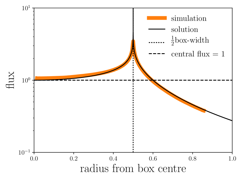
Figure 4: Flux as a function of radius from an emitting sphere. TREVR’s solution for background source particles distributed in a spiral on a sphere of radius $R=0.5$ (black dotted line) are plotted as the thick orange line. The analytical solution given by Equation 24 is plotted as a thinner black line on top of the numerical solution. A constant flux of one is plotted by the black dashed line and is achieved in the inner most region of this simulation at around $R\lesssim 0.05$.

Note that due to the logarithm in Equation 24, the flux is nearly constant at small radii. Since most cosmological zoom in simulations only consider gas at a fairly small radius, this setup of background sources is an acceptable method of imposing a background flux. A benefit of this method is that we can use all of the existing machinery already described, and only have to add background star particles as the source of the background radiation. Also note that the simulation flux is over estimated near the shell. When merging background sources which are all located on the surface of a sphere, the merged centre of luminosity will always be at a smaller radius than the sphere radius. This can be remedied by forcing merged background sources to always be located on the sphere.

2.3 Implementation Specifics

As mentioned earlier, TREVR is not specific to either Gasoline or SPH. However, in this subsection we introduce Gasoline and the specifics of TREVR’s implementation in Gasoline.

Gasoline is a parallel smoothed particle hydrodynamics code for computing hydrodynamics and self-gravity in astrophysics simulations. It employs a spatial binary tree that is built by recursively bisecting the longest axis of each cell. In the current version of TREVR, a separate tree is built for computing radiative transfer. For development purposes, this is a convenient choice, but adds extra cost and in the future a single tree should be adopted, particularly as tree building becomes a significant cost with adaptive timestepping. A special requirement for the radiation tree is that it fills all space to correctly estimate absorption due to ray intersections. Both the gravity and hydrodynamics trees squeeze cell bounds to the furthest extents of particles within the cell to optimize intersection tests which creates gaps between cells.

In the regular tree building phase, Gasoline assigns an “opening radius” about a cell’s centre of mass to each cell in the tree. This radius is

$$r_{\rm open}=\frac{2B_{\rm max}}{\sqrt{3}\,\theta_{\rm open}},$$ (25)

where $B_{\rm max}$ is the distance from the centre of mass of particles within the cell to the furthest particle from the centre of mass. However, since we are using space-filling cells for the radiation tree, it is necessary to define $B_{\rm max}$ instead as the distance to the furthest vertex of the cell.

The initial method used to compute cell densities during the tree build process was to divide the sum of masses of particles within the cell by the cell volume,

$$\rho_{\rm cell}=\frac{\sum_{i}m_{i}}{V_{\rm cell}}.$$ (26)

However, during testing at high levels of refinement we found that the error began to increase slightly with increasing refinement accuracy beyond a certain level. This was because when refining down to the bucket level, $N_{\rm B}=10$ was small enough to introduce Poisson noise in the density estimate. This propagated as errors in the computed radiation field, noticeable as noise in otherwise uniform density distributions. To remedy this for particle-based methods, each cell uses a volume-weighted average of the particle densities,

$$\rho_{\rm cell}=\frac{\sum_{i}m_{i}}{\sum_{i}{\frac{m_{i}}{\rho_{i}}}}.$$ (27)

As noted in Section 2.2.3, when sub-bucket level refinement is required a ray trace similar to that of SPHRay is performed. In this method, all particles in a cell are projected down to the ray, and an impact parameter, $b$, is calculated (See Figure 5).

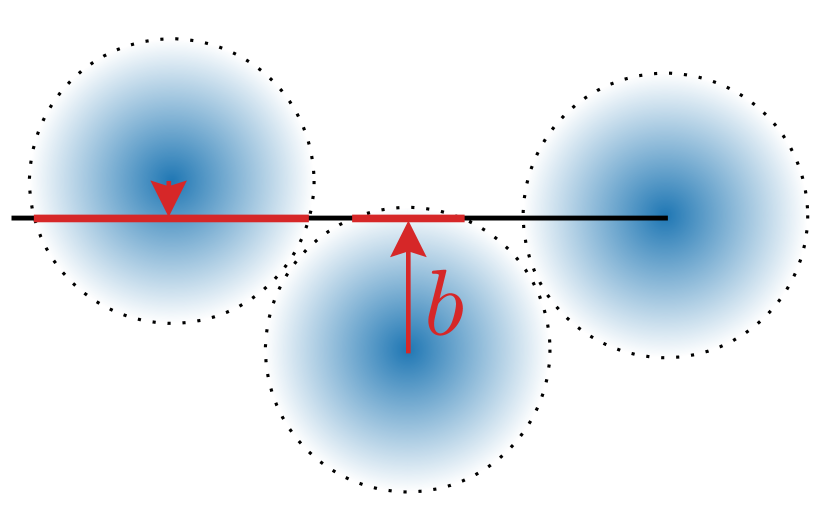
Figure 5: The ray tracing scheme employed is similar to that of Altay et al. (2008). In this scheme, the photons are diminished by the optical depth along each particle’s density field. The receiving particle at the termination of the ray does not block photons to itself. Otherwise, the front half of the particle would diminish the incoming photons without actually having absorbed them.

Since the density field of an SPH particle varies with radius due to the smoothed nature of SPH, an (pre-calculated) integral over the smoothing kernel, $W$, must be used. Thus, Equation 7 becomes

$$\tau_{i}(s)=\left(m_{i}\int W\right)\kappa_{i}ds,$$ (28)

where $m_{i}\int W$ represents the effective density along the particular ray and $ds$ is the section of the ray intersected by the particle’s smoothing length (red line segments in Figure 5). Note that for the receiving particle, its own density field does not contribute to the overall optical depth. To see why this must be the case, consider the case where a single particle is optically thick. If the front half of the particle contributed to absorption, the flux calculated at the centre would be effectively zero, and the particle would incorrectly report no heating or ionization. This is essential for correct ionization fronts such as in the Strömgren test of Section 3.3.

The implementation operates in parallel in exactly the same way as the gravity solver, as described in the original Gasoline paper by locally caching copies of remote tree cells and particles.

3 Code Tests

3.1 Sinusoidally Perturbed Glass

3.1.1 Initial Conditions

To test the accuracy and general scaling of the algorithm we require an initial condition (IC) that is representative of a typical use case. For this we have created a novel IC comprised of a unit length glass cube of $N$ SPH gas and $N$ star particles whose positions have been perturbed by 24 random sinusoidal modes. The initial glass of particles is built from copies of the $16^{3}$ glass used to create ICs for other tests of Gasoline (Wadsley et al., 2017). The total mass of gas particles is one, and the opacity of each particle is also one. This results in an optical depth across the width of the box of $\sim$1, making the simulation volume marginally optically thin overall with dense, optically thick filamentary structure and underdense voids qualitatively similar to the cosmic web. Each star particle is assigned a luminosity of one. A slice of this density distribution is plotted in Figure 6. Appendix A contains a detailed explanation of how this IC was created including a table of modes used.

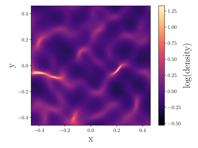
Figure 6: A $z$-plane slice of the sinusoidally perturbed glass IC. The optical depth along the longest filament in the slice (left, just below $y=0$) is $\tau\approx 4$. The optical depth across the largest void (above the aforementioned filament) is $\tau\approx 0.1$.

3.1.2 Opening Angle

The opening angle criterion’s effect on accuracy and cost was tested by ray tracing the optically thin, sinusoidally perturbed glass IC with $\theta_{\rm open}$ varying between 0 and 1. The results of this test are plotted in Figure 7. The measure of cost is plotted as the total number of rays, $N_{\rm rays}$, computed per resolution element on the left $y$-axis. The number of rays is equivalent to the number of radiation sink-source interactions computed in a simulation timestep. Using rays as a measure of cost allows us to isolate the effects of the opening criterion on cost. On the right $y$-axis we have plotted the root mean squared (RMS) fractional error relative to the radiation field computed with $\theta_{\rm open}=0$. This test was run with $\tau_{\rm ref}=0.1$ and $N=64^{3}$ star and gas particles.

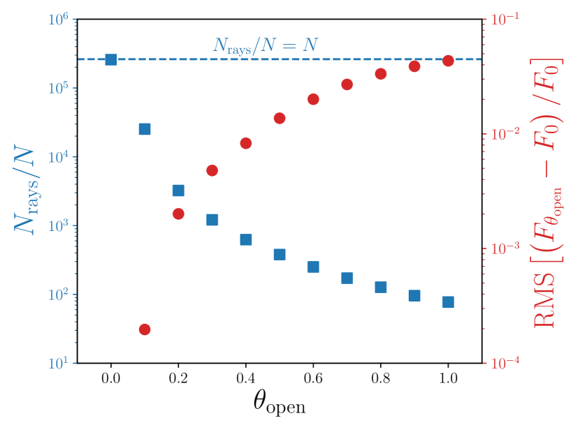
Figure 7: A plot of cost and accuracy as a function of opening angle. The number of rays computed per resolution element is plotted in blue, on the left $y$-axis with square markers. The blue dashed line shows $N_{\rm rays}/N=N$ at an opening angle of $\theta_{\rm open}=0$, meaning TREVR can perform an $\mathcal{O}\left(N^{2}\right)$ ray trace if desired (omitting the cost of absorption). The RMS error in flux relative to $\theta_{\rm open}=0$ is plotted in red, on the right $y$-axis with circular markers.

At $\theta_{\rm open}=0.75$, the value used in all other tests and the default value for $\theta_{\rm open}$ in many gravity solvers, 200 rays are computed per resolution element with an RMS fractional error of 3%. To achieve a RMS fractional error of about 1%, we suggest that a lower opening angle of approximately $\theta_{\rm open}=0.45$ should be used. $\theta_{\rm open}=0.45$ costs only 500 rays per resolution element, which is still much less than interacting with all $64^{3}$ ($2.6\times 10^{5}$) sources.

3.1.3 Refinement Criterion

Testing the refinement criterion is similar to testing the opening angle criterion. Again, the sinusoidally perturbed glass IC was simulated but now with a varying $\tau_{\rm ref}$ value. The results of this test are plotted in Figure 8. The min and max values for $\tau_{\rm ref}$ were chosen to show how the cost curve flattens out on either side: the left hand side being where refinement has occurred down to the bucket level and the right hand side being where refinement is never done. An opening angle of 0.75 was used and $N=64^{3}$ for both star and gas particles. Cost is plotted on the left $y$-axis and RMS fractional error on the right $y$-axis. The measure of cost is now the number of ray segments per resolution element, since the refinement criterion controls the number of ray segments a single ray is broken up into. The measure of accuracy is again the RMS fractional error, but now relative to the radiation field computed with $\tau_{\rm ref}=1\times 10^{-8}$, which ensures maximum resolution everywhere.

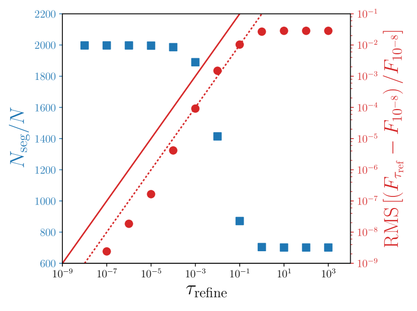
Figure 8: Algorithmic cost and accuracy as a function of refinement criterion. The number of ray segments computed per resolution element is plotted in blue, on the left $y$-axis with square markers. The RMS error in flux relative to $\tau_{\rm ref}=10^{-8}$ is plotted in red, on the right $y$-axis with circular markers. Lines of ${\rm error}=\tau_{\rm ref}$ and ${\rm error}=\tau_{\rm ref}/10$ are plotted as red solid and dotted lines respectively. The upper line represents maximum allowable error per ray segment. The RMS relative error roughly follows the lower line, an order of magnitude lower.

At $\tau_{\rm ref}=0.1$, 1% RMS fractional error is achieved with a cost of approximately 850 ray segments computed per resolution element (including all rays), less than half the cost of refining all the way to the bucket level. Note also that RMS fractional error as a function of $\tau_{\rm ref}$ behaves predictably, lying below the error = $\tau_{\rm ref}$ line and roughly following the error = $\tau_{\rm ref}/10$ line plotted in Figure 8. This shows that the error per ray segment is well controlled by our refinement criterion and considerably lower than $\tau_{\rm ref}$ on average.

The RMS fractional error plateaus at 2-3% in this test. In this particular implementation of TREVR, the walk along the ray goes up from both the bucket where the radiation sink resides and the opened cell where the source resides, to the top of the tree. This built in level of refinement is the reason for the low maximum error. Other implementations, that walk the ray top down or up and then back down the tree, would need to rely more, or solely, on the refinement criterion. In principle, such a method could perform better than $\mathcal{O}\left(N\log^{2}N\right)$.

3.1.4 Scaling

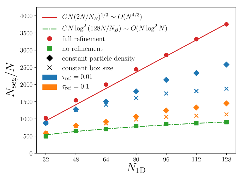
Figure 9: Cost, quantified as the number of computed ray segments per resolution element, is plotted as a function of $N_{\rm 1D}=N^{1/3}$. TREVR’s theoretical upper and lower scaling bounds are plotted as red (solid) and green (dash-dot) lines respectively. The corresponding simulation data points are plotted as red circles and green squares. Simulation data points intermediate to the scaling bounds are plotted as combinations of two parameters - refinement criterion parameter value and the type of scaling. Tests run with a refinement criterion of $\tau_{\rm ref}=0.1$ are coloured orange and make up the lower two sets of intermediate data. The upper sets of intermediate data, coloured blue, are tests run with $\tau_{\rm ref}=0.01$. Diamond markers denote weak scaling tests and $\times$ shaped markers denote strong scaling tests.

To test cost scaling as a function of $N$, we hold $\theta_{\rm open}$ constant at 0.75 and vary $N$ between $32^{3}$ and $128^{3}$ in steps of $N_{\rm 1D}=16$ for both gas and star particles. To substantiate the best and worst-case theoretical scaling claims made in Equations 23 and 21 respectively, the sinusoidally perturbed glass IC was simulated with $\tau_{\rm ref}=1\times 10^{6}$ to ensure refinement was never performed and with $\tau_{\rm ref}=0$ to ensure refinement was always performed down to the bucket level. Data from these tests and the fitted theoretical lines are plotted in Figure 9 and correspond very closely to each other. Note that the only parameter used to fit the theoretical lines is a constant factor multiplying Equations 21 and 23.

Scaling behaviour between the upper and lower limits was probed in two ways. Firstly, simulations were run with $\tau_{\rm ref}$ values of 0.1 and 0.01. Secondly, strong and weak scaling cases were simulated. The strong scaling case being where the simulation volume was held constant and particle number increased. This is analogous to increasing the resolution in a standard galaxy simulation. The weak scaling case is the opposite, in which the simulation volume is increased and particle density is held constant. This is analogous to simulating larger and larger cosmological boxes to achieve larger statistical samples. Note that the previously described tests of the upper and lower scaling bounds were only run as strong scaling tests.

Results from these tests are shown in Figure 9. There are two interesting things to note. Firstly, with refinement we can maintain a scaling quite similar to the best case of $N\log^{2}{N}$ in this representative test. Secondly, the strong scaling case, which is typically the harder case to scale effectively in other respects (e.g. parallelism), scales better than the weak scaling case. The strong scaling data is closer to $N\log^{2}{N}$ and costs less than the weak scaling case for the same $N$. This is because the larger boxes in the weak scaling case have larger total optical depths and thus require more ray segments to achieve the same flux accuracy.

3.2 Isothermal Spheres

3.2.1 Initial Conditions

The sinusoidally perturbed glass IC tests a generally optically thin, smooth density distribution. This is a good proxy for many astrophysical cases of interest, such as late stage galaxy evolution. We now show how well TREVR’s refinement criteria can handle compact, optically thick features. We created an IC featuring a single radiation source positioned in the top left corner and four spheres with $1/r^{2}$ density profiles (mimicking self-gravitating dense objects) embedded in a uniform region, with opacity and density both set to one. The four isothermal spheres have a density distribution given by

$$\rho(r)=\frac{\rho_{0}\epsilon^{2}}{r^{2}+\epsilon^{2}},$$ (29)

where the softening length is $\epsilon=0.002$ and the central density, $\rho_{0}=626$. The IC was made starting with a uniform density glass of fixed mass particles. SPH gas particles were added inside the sphere radii. To do this the uniform glass was duplicated and associated with negative radii for a given sphere. A mapping from this initial space (including both negative and positive radii) to positive radii in the final space was calculated analytically that gave the desired isothermal density profile for that sphere while maintaining a glass-like distribution. Any duplicated particles that did not map to positive radii were then deleted. This technique is able to embed arbitrarily large non-linear density perturbations in any uniform density glass.

The chosen parameters set the maximum optical depth through a sphere to $\tau_{\rm max}=4$ (a 98% reduction in flux) and the density at the edge of the spheres to one, matching the unit density of the uniform background. The isothermal spheres have a radius of 0.05 of the box length and are shown as grey circles in Figure 10.

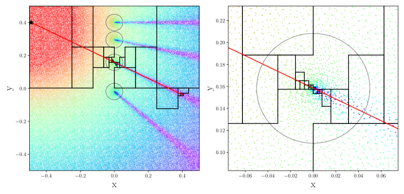
Figure 10: Left: TREVR’s adaptive refinement criterion (at $\tau_{\rm ref}=0.1$) resolving isothermal spheres in a uniform environment. Particles in a slice along the $z$-plane of the isothermal spheres IC are coloured by the logarithm of their flux value (high - low flux, red - purple). The red line represents the ray traced from the radiation source (black star) to the receiving cell. Black rectangles represent the spatial boundary of the tree cells used compute the optical depth of the intersecting ray segment. Right: A zoom-in of the sphere intersected by the ray to focus on the refinement across the sphere itself.

The spheres are centred on the $x$ and $z$ axis with $y$ coordinates given by

$$y_{i}=0.75-1.3^{-(4-i)},$$ (30)

where $i$ runs from zero to three. The radiation source, denoted by the black star in Figure 10, is located at $x=0.49$, $y=y_{0}$ and $z=0$. The total number of particles in the IC is $N=4,111,624$.

The spheres produce shadows away from the source. Accurate shadows can only be cast if the sharply peaked spheres are resolved correctly by the refinement criterion. Errors arising specifically in the optically thick regime can be isolated by looking at particles in shadow.

3.2.2 Refinement Criterion

The effects of the refinement criterion on accuracy and cost in this test were analyzed similarly to the previous test. The main addition in Figure 11 is that the subset of particles in shadow has its RMS fractional error plotted separately to highlight the refinement criterion’s performance in the optically thick regime.

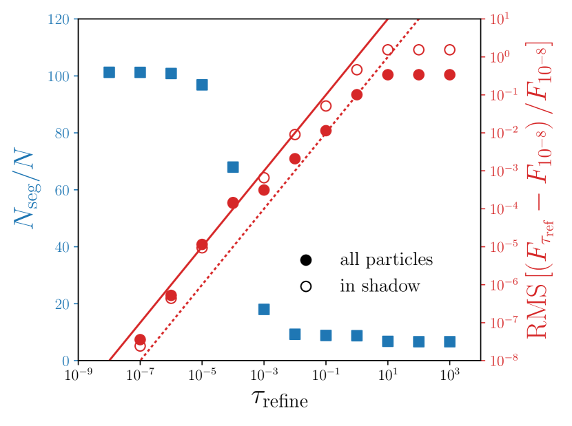
Figure 11: A plot of cost and accuracy as a function of refinement criterion. The number of ray segments computed per resolution element is plotted in blue, on the left $y$-axis with square markers. The RMS error in flux relative to $\tau_{\rm ref}=10^{-8}$ is plotted in red, on the right $y$-axis with circular markers. Lines of ${\rm error}=\tau_{\rm ref}$ and ${\rm error}=\tau_{\rm ref}/10$ are plotted as red solid and dotted lines respectively. Solid circular markers represent RMS relative errors computed on all resolution elements and empty markers represent only the resolution elements that fall in shadow. The in-shadow errors are larger for looser refinement criterion, continuing to follow the ${\rm error}=\tau_{\rm ref}$ line.

As before, $\tau_{\rm ref}=0.1$ achieves an overall RMS fractional error of 1% with very little cost. However, when restricting the focus only to those particles in shadow, the same refinement parameter produces much higher errors ($\sim$ 8%). Decreasing the refinement parameter by an order of magnitude to $\tau_{\rm ref}=0.01$ predictably decreases the RMS fractional error on particles in shadow to 1%, with a negligible increase in the cost from that at $\tau_{\rm ref}=0.1$ as most of the volume is fairly optically thin and does not need to be refined in either case.

The $\rm{error}=\tau_{\rm ref}$ and $\rm{error}=\tau_{\rm ref}/10$ lines are again plotted in Figure 11. For the most part the RMS fractional error is contained between these lines, with only two of the in-shadow points at $\tau_{\rm ref}=1\times 10^{-5}$ and $1\times 10^{-4}$, and one of the all-particle points at $\tau_{\rm ref}=1\times 10^{-4}$ sitting marginally above the $\rm{error}=\tau_{\rm ref}$ line. The error bound represented by Equation 19 is tighter for this test, with the overall error closer to $\tau_{\rm ref}$.

The isothermal spheres test is an especially difficult test as there is only one source, and the errors are more systematic. Thus, the errors are less likely to cancel the way random errors often do, for example, with many sources. Such random cancellations mean that overall errors for TREVR typically perform better than the bound given by Equation 19.

The isothermal spheres test is useful as it is representative of structure commonly found in astrophysics and because it has an analytic solution. However, in SPH it is difficult to represent sharp density gradients with discrete resolution elements. This causes in-shadow particle flux errors relative to the analytic solution (not shown) to be up to an order of magnitude higher than the errors relative to the $\tau_{\rm ref}=10^{-8}$ simulation plotted in Figure 11. These errors are associated with the discrete representation of the density profile rather than the radiative transfer method.

3.3 Strömgren Sphere Test

3.3.1 Strömgren Sphere Theory

The Strömgren sphere is a theoretical ionized sphere of gas first discussed by Bengt Strömgren in 1938 (Strömgren, 1939) as a model of the HII region around a hot, young star. The theoretical ICs consist of a uniform density cloud of neutral hydrogen gas with an ionizing source of radiation at its centre. As photons from the source ionize the hydrogen, the optical depth of the gas decreases and so the ionizing photons are able to travel further and further from the source creating a moving ionization front. Eventually, a radius is reached such that the total ionization rate equals the recombination rate. At this point, the front reaches an equilibrium, creating a stable sphere of ionized hydrogen. The Strömgren sphere test has become a common code test in RT methods papers (Pawlik & Schaye, 2008, 2011; Petkova & Springel, 2011) and comparison papers (Iliev et al., 2006, 2009), as it is a simple test of a method’s ability to resolve ionization fronts and achieve equilibrium behaviour that may be compared with analytic results.

The equilibrium radius or Strömgren radius, $R_{S}$, is the radius at which the ionization and recombination rates are equal (e.g. Tielens, 2005),

$$R_{S}=\left(\frac{3}{4\pi}\frac{\dot{N}_{\gamma}}{\alpha\,n^{2}_{H}}\right)^{1/3},$$ (31)

where $\dot{N}_{\gamma}$ is the source luminosity in photons per second, $\alpha$ is the recombination rate and $n_{H}$ is the hydrogen number density. One can also solve for the radius as a function of time (e.g. Spitzer, 1978),

$$R(t)=R_{S}\left[1-\exp\left(t/t_{\rm rec}\right)\right]^{1/3}$$ (32)

where $t_{\rm rec=1/{n_{H}\alpha}}$ is the recombination time of the gas. The above derivation assumes a “sharp” ionization front, meaning the transition from ionized to neutral hydrogen occurs across an infinitesimally thin region. In practice, there is a finite transition region and structure interior to the Strömgren radius. In order to solve for the non-sharp ionization front we must consider the hydrogen ionization equation

$$\frac{\partial n_{\rm HII}}{\partial t}=c\sigma n_{\rm HI}n_{\gamma}-\alpha n_{\rm e}n_{\rm HII},$$ (33)

where $n_{x}$ is the number density of species $x$, HI and HII label neutral and ionized hydrogen respectively, $\gamma$ denote photons, $\sigma$ is the ionization cross-section, $c$ is the speed of light and $\alpha$ is the recombination rate. Note that we have omitted collisional ionization in Equation 33, which is customary for this test, however it should be included in general. By integrating the ionization equation and the flux equation with absorption (Equation 9), we get a solution for the relative abundance of HI and HII as a function of radius and as a function of time (Osterbrock & Ferland, 2006). In the following tests, we include both the theoretical sharp front solution and non-sharp front solutions from the Iliev et al. (2006) comparison paper to compare to our results. We also attempt to duplicate the ICs of Iliev et al. (2006) as closely as possible. It should be noted that a time-step limit associated with ionization and temperature changes is required to correctly follow ionization fronts. We employed the pre-exisiting ionization, heating and cooling integrator in Gasoline with no changes other than using the standard coefficient values for these tests described below.

3.3.2 The Isothermal Strömgren Sphere

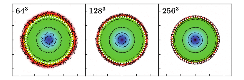
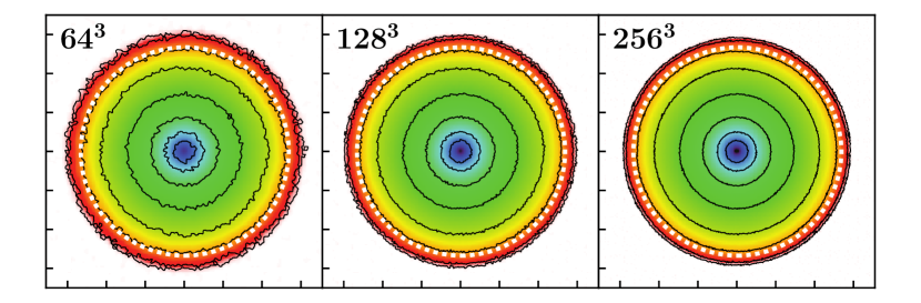
Figure 12: A slice through the $z$-plane of the isothermal Strömgren sphere test at $t=30$ Myr (top row) and $t=500$ Myr (bottom row). Particle resolutions increase from left to right denoted by the $N$ value in the top left corner of each pane. Axis ticks are spaced 2 kpc apart, so note that ionized spheres in the top row are a fraction of the volume and particle resolution of spheres in the bottom row. The colormap represents neutral fraction, $\rm x$, and is similar to that of Pawlik & Schaye (2008) and Pawlik & Schaye (2011) to allow for ease of comparison. We use the same contour levels: $\rm x$ = 0.9, 0.5, $\log\rm x$ = -1, -1.5, -2, -2.5, -3 and -3.5. The white dashed line is a circle of radius given by Equation 32, the sharp, time dependent solution to the isothermal Strömgren sphere.

In the simplest case, the ionizing source is assumed to emit monochromatic photons at 13.6 eV and the gas is held at fixed temperature of $T=10^{4}$ K. We refer to this case as the isothermal Strömgren sphere. The medium is initially neutral with a uniform density of $n_{\rm HI}=10^{-3}$ $\rm cm^{-3}$. We use an ionization cross-section of $\sigma=6.3\times 10^{-18}$ $\rm cm^{-2}$ and a recombination rate of $\alpha=2.59\times 10^{-13}$ $\rm cm^{-3}$ $\rm s^{-1}$, typical of $10^{4}$ K gas. An ionizing source is turned on at $t=0$ and emits at a rate of $\dot{N}_{\gamma}=5\times 10^{48}$ photons $s^{-1}$. These values yield a Strömgren radius of $R_{S}=5.38$ kpc and a recombination time of $t_{\rm rec}\approx 125$ Myr.

We note that Iliev et al. (2006) use a 6.6 kpc cube which only contains a single octant of the Strömgren sphere for their testing. We have opted to use an 16 kpc cube, increasing the maximum front radius to 8 kpc to avoid any edge effects (the sphere gets close to the edge of the box for some codes in the above paper). In order to aid comparison, we still normalize radius values to 6.6 kpc, as is done in Iliev et al. (2006). As well, we have not imposed a floor on the HII fraction of 0.001, as was done in their paper. Because the resolution used in the Iliev et al. (2006) comparison paper was never specifically given, we have opted to run the test with $N=64^{3}$, $128^{3}$ and $256^{3}$ particles to represent the entire sphere. These resolutions correspond to single octant resolutions of $N=32^{3}$, $64^{3}$ and $128^{3}$ in Iliev et al. (2006). Varying the number of particles also allows us to invesitgate at how TREVR converges with resolution. We have run our Strömgren sphere tests with fixed accuracy parameters of $\theta_{\rm open}=0.75$, $\tau_{\rm ref}=0.1$.

Figure 12 is a slice through the $z$-plane of the simulation. The colour map shows the neutral fraction. The contour levels and colour map have been chosen to closely mimic Figure 6 in both Pawlik & Schaye (2008) and Pawlik & Schaye (2011). We have done this to highlight a key benefit that ray tracing codes such as TREVR have over photon packet propagation methods such as TRAPHIC: isotropy. At the same $N=64^{3}$ particle resolution TREVR is more spherically symmetric than TRAPHIC, even with their use of Monte-Carlo re-sampling. Furthermore, TREVR outperforms TRAPHIC in this aspect even at early times (top panels in Figure 12). Here the interior of the sphere is represented by 3.3 times fewer particles than the late time Strömgren spheres plotted in the TRAPHIC papers.

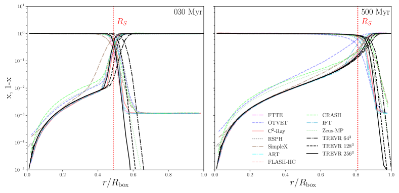
Figure 13: Spherically averaged neutral and ionized fraction ($\rm x$ and $\rm 1-x$) profiles for the isothermal Strömgren sphere test during the fast expansion (left) and equilibrium (right) stages. Radius on the $x$-axis is normalised by a box length of 6.6 kpc for comparison with plotted solutions from the Iliev et al. (2006) comparison paper.

Figure 13 is a plot of neutral/ionization fraction as a function of radius from the Strömgren sphere centre. The sharp Strömgren radius is plotted as well as non-sharp solutions from all codes presented in Figure 8 of Iliev et al. (2006). TREVR tends to over-ionize at lower resolutions, but recreates the ionization profile quite well overall. At 30 Myr we converge with resolution to the sharp solution. At 500 Myr we converge to the non-sharp numerical solutions, which also over-ionize relative to the sharp solution at late times. Overall, the two higher resolution solutions are within the scatter of the non-sharp solutions of the codes presented in Iliev et al. (2006).

3.3.3 The Non-Isothermal Strömgren Sphere

The above test assumed the hydrogen gas was isothermal and that all incident photons had the same energy. In reality, photons range across many wavelengths with differing cross-sections at each wavelength. Absorption results in heating as well, which affects many gas properties including the recombination rate.

We reran the Strömgren sphere test, but this time the incident photons are assumed to be from a black body with a temperature of $10^{5}$ K. The cross-section is now photon energy weighted, giving $\sigma=1.63\times 10^{-18}$ $\rm cm^{-2}$. The gas has an initial temperature of 100 K and the recombination rate is a function of temperature set by

$$\alpha(T)=2.59\times 10^{-13}\left(\frac{T}{10^{4}\hskip 5.0pt{\rm K}}\right)^{-0.7}\hskip 5.0pt{\rm cm}^{-3}\hskip 5.0pt{\rm s}^{-1}$$ (34)

to match Petkova & Springel (2009). This test includes heating due to absorption and cooling due to recombination $\Delta_{r}$, collisional ionization $\Delta_{ci}$, line cooling $\delta_{l}$, and Bremsstrahlung radiation $\Delta_{B}$. The rates are taken from Cen (1992) in order to match Petkova & Springel (2009).

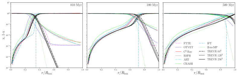
Figure 14: Spherically averaged neutral and ionized fraction ($\rm x$ and $\rm 1-x$) profiles for the non-isothermal Strömgren sphere test during the fast expansion (left), slowing down (middle) and equilibrium (right) stages.

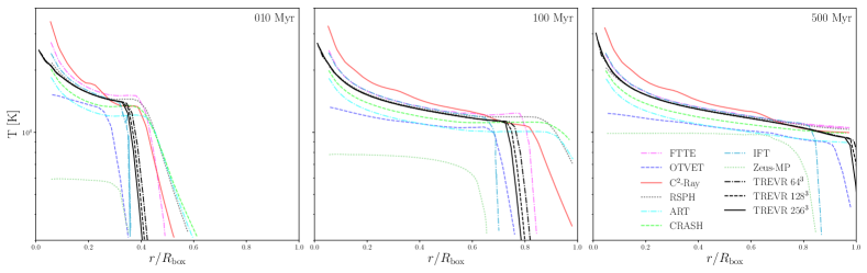
Figure 15: Spherically averaged temperature profiles for the non-isothermal Strömgren sphere test.

Figures 14 and 15 show the neutral/ionized fraction and temperature respectively as a function of radius at $t=$ 10, 100 and 500 Myr. These times represent the fast expansion stage, slowing down stage and final equilibrium Strömgren sphere respectively. We have plotted numerical solutions from Figures 16 and 17 in Iliev et al. (2006) for comparison. Again, TREVR recreates these profiles quite well. TREVR gives a somewhat large sphere radius which is due in part to the ionization code rather than the radiation method. The temperature profile lies in the middle of the scatter of the Iliev et al. (2006) solutions. We note that for this test different codes employed different assumptions about radiation bands and ionization treatments which makes detailed comparisons difficult.

4 Discussion And Conclusions

In this paper we have presented TREVR, a practical and efficient, general purpose algorithm for computing RT in astrophysics simulations. For a RT method to be these things it must remain efficient with large numbers of resolution elements and radiation sources, compute the radiation field to a desired level of accuracy and handle density and opacity distributions representing the optically thick, thin and intermediate regimes.

TREVR’s ability to scale feasibly with $N$ and $N_{\rm source}$ is achieved by reducing all three of the cost multipliers of an $\mathcal{O}\left(N_{\rm sink}N_{\rm source}N^{1/3}\right)$ naive ray trace:

1. Reverse ray tracing allows for the use of adaptive timesteps. The initial dependence on $N_{\rm sink}\sim N$ resolution elements is reduced to just the active radiation sinks (i.e. gas). $N_{\rm sink}$ is effectively hundreds of times smaller than $N$ when averaged over a large number of substeps.

2. Source merging based on an opening angle criterion reduces the linear dependence on $N_{\rm source}$ to $\log N_{\rm source}$.

3. By adaptively reducing the resolution of rays via TREVR’s novel refinement criterion, the $N^{1/3}$ cost of computing the optical depth along a ray can be reduced to $\log N$, while maintaining a specified level of accuracy.

In Section 2.2 we theoretically predicted TREVR’s $\mathcal{O}\left(N_{\rm sink}\log N_{\rm source}\log N\right)$ scaling behaviour. In the general case, represented by the perturbed glass test case with accuracy parameters of $\tau_{\rm ref}=0.1$ and $\theta_{\rm open}=0.75$ (Figures 7, 8 and 9), we have shown that TREVR can indeed scale as predicted whilst achieving $\sim 1\%$ error. We also note that better than $\mathcal{O}\left(N_{\rm sink}\log N_{\rm source}\log N\right)$ scaling (i.e. closer to $\mathcal{O}\left(N_{\rm sink}\log N_{\rm source}\right)$) could be achieved for a medium with low optical depths via a more aggressive, top-down ray walk with our refinement criterion.

The only general ray-tracing code we are aware of with similar scaling is TREERAY (Wünsch et al., 2018). TREERAY does not use an adaptivity criterion and has a fixed number of rays. This rather rigid approach has a benefit which is that the source and absorption walks can be combined to given an overall $\mathcal{O}\left(NlogN\right)$ scaling, albeit without error controls and limited directional accuracy (e.g. for shadowing). TREERAY, as currently implemented in FLASH, uses a global timestep and is thus unable to take advantage of the large speed-ups reverse ray tracing can achieve via adapative timestepping. However, this is not a limitation intrinsic to the TREERAY method itself.

We note that the opening angle criterion is guaranteed to limit errors in the low optical depth regime. However, with absorption, it sets an effective angular resolution below which shadows from distinct sources would merge. As shown in the tests (see particularly sections 3.1), this does not adversely effect the RMS errors with absorption in cases with many sources. However, it can adjust the location of shadow edges (which is where most of the error resides). In the case of a few strong sources, the user could employ a stricter merging criterion (or one based on brightness) and have arbitrarily good angular resolution with relatively little cost as demonstrated in section 3.2.

In plots of accuracy as a function of $\tau_{\rm ref}$ (Figures 8 and 11) we have also shown that TREVR’s refinement criterion provides a predictable bound on accuracy, as we found the RMS relative error is $\propto\tau_{\rm ref}$ and the RMS errors do not exceed $\tau_{\rm ref}$.

This behaviour enables TREVR to reap the benefits inherent in instantaneous ray tracing methods whilst still being practical and general. For example, we can use any convenient timestep rather than being limited by the speed of light. Directional accuracy is another one of these benefits as is apparent in the sharp shadows cast in the isothermal spheres test (Figure 10). Low levels of noise and anisotropy are also benefits compared with evolutionary methods as is apparent in the Strömgren sphere test (Figure 12).

In the version of TREVR as currently implemented, there are still some problems not easily handled. First, in any completely optically thick medium where high accuracy is required our method will result in worst case scaling of $\mathcal{O}\left(N_{\rm sink}\,N^{1/3}\right)$ (characterized in Section 2.2.3). At face value this limits TREVR to solving only post-reionization cosmology or similar problems that are largely optically thin. However, in optically thick media most sources contribute nothing to the local radiation field. In such cases TREVR could easily terminate ray traces that are found (e.g. early in the optical depth sum when $\tau$ exceeds a threshold) or predicted (based on information from prior timesteps) to contribute little to no intensity to the final radiation field. These types of optimizations could also improve the weak scaling case.

A second problem is periodicity. Our method of a sphere of background sources providing a constant central background flux is adequate for isolated objects, but in the context of large cosmological boxes, such as reionization calculations, periodic boundaries are required. In such contexts, light travel times and redshifting are also potentially important. Such factors could be included in principle and this is a potential direction for future work.

Finally, there is the important issue of complex sources. Consider a group of sources that meet the opening criterion and are merged, but are also contained within a region that has clumpy, opaque structures. Depending on the location of the merged centre of luminosity relative to the opaque clumps, the amount of radiation that escaped the merged source cell could vary significantly from that computed by the current algorithm. Such cases would require that the opening criterion take the effect of nearby absorbers into account, potentially using the information regarding the variance in $\alpha$ already recorded for each cells. Such extended opening and refinement criterion are the subject of ongoing investigations.

In addition to the above, future work could also include implementing scattering. The process of scattering can be recast as an absorption, followed by an immediate re-emission of photons. Thanks to the $\log(N_{\rm source})$ scaling with radiation sources, this process can be implemented by considering resolution elements (SPH gas particles in our case) as sources of radiation without changing the scaling of the method.

A consequence of assuming an infinite speed of light is that radiation sinks will not see light as it was when emitted in the past but as the source appears at the current time. This is easy to remedy, as we have both the age of the source as well as the distance travelled by the photons. We can then age the radiation sources with respect to the receiving resolution element, such that the received photons are representative of the luminous source as it was.

Currently, TREVR only computes the radiation field in specific bands. TREVR can handle many bands of radiation with a small constant multiplier added to the cost. However, it may be advantageous to evolve the spectral shape over distance using an opacity which is a function of wavelength where the absorption is provided by a relatively simple or easily characterized set of species. This would also enable us to incorporate redshifting effects important for the evolution of large boxes over cosmological time periods.

J. Wadsley and H. M. P. Couchman would like to acknowledge the support of NSERC.

Appendix A Creating the Sinusoidally Perturbed Glass IC

To create our gently varying density distribution for the many source tests, we modify positions of particles in a glass IC by adding the sum of 24 sinusoidal modes to the initial particle positions as in Equation 35 below

$$\vec{r}=\vec{r}_{\rm 0}+\sum_{i=1}^{24}\frac{1}{275}\sin\left(k_{x,i}r_{x}+k_{y,i}r_{y}+k_{z,i}r_{z}+\phi_{i}\right),$$ (35)

where $\vec{r_{0}}$ is the particles initial position in the glass and $\vec{r}$ is its perturbed position in the final distribution. The $\vec{k_{i}}$ and $\phi_{i}$ values are listed in Table 1 in order to facilitate reproduction of the scaling tests. Both gas and star particles have the same density distribution. However, the initial glass was flipped for the star particles by reassigning $x$,$y$ and $z$ coordinates via

$$x_{\rm star}=y_{\rm gas},\hskip 5.0pty_{\rm star}=z_{\rm gas},\hskip 5.0ptz_{\rm star}=x_{\rm gas},$$ (36)

to prevent the particles from occupying the same position in space.

Table 1: Randomly generated $\vec{k}$ and $\phi$ values used in generating the sinusoidally perturbed glass IC.

$i$	$k_{x,i}$	$k_{y,i}$	$k_{z,i}$	$\phi_{i}$
01	$-$3.918398	$+$1.727743	$-$4.476095	0.829776
02	$-$3.681821	$-$4.619688	$+$4.865007	3.891157
03	$-$4.831801	$+$3.769470	$+$0.567451	3.668730
04	$-$2.298279	$+$1.501757	$+$4.716946	1.528348
05	$-$0.289974	$-$3.097958	$+$1.270028	4.113001
06	$+$1.262943	$-$1.661726	$-$2.600413	4.481799
07	$+$1.588224	$+$4.072259	$+$0.616444	2.971965
08	$-$2.253394	$-$2.806478	$+$2.749155	0.442241
09	$-$1.432569	$+$3.324710	$+$4.842991	2.871989
10	$+$1.287742	$-$4.575517	$-$4.001723	1.727810
11	$+$4.769704	$+$0.540096	$-$4.203839	5.872117
12	$-$3.013200	$-$1.871251	$-$2.514416	1.574008
13	$-$4.588620	$+$4.384224	$+$1.246849	1.985715
14	$-$0.372817	$+$0.195243	$+$4.074056	6.248739
15	$-$1.842232	$+$0.901598	$-$4.453613	6.273336
16	$+$1.986937	$-$1.037650	$+$1.958888	2.177783
17	$-$1.748485	$-$1.386029	$+$3.755833	0.532604
18	$+$4.852406	$-$3.272506	$+$0.826504	5.525470
19	$+$3.663293	$-$4.597598	$-$0.890135	4.528870
20	$-$1.720903	$+$2.726011	$+$3.192427	3.875610
21	$+$4.973332	$+$4.777182	$-$2.515792	0.406737
22	$+$0.057238	$-$2.972427	$-$1.828550	4.125258
23	$+$0.938234	$-$0.487023	$-$2.755097	1.335299
24	$+$1.943361	$+$0.388178	$-$3.783953	4.774938

References

- Agertz et al. (2013) Agertz O., Kravtsov A. V., Leitner S. N., Gnedin N. Y., 2013, ApJ, 770, 25
- Altay & Theuns (2013) Altay G., Theuns T., 2013, MNRAS, 434, 748
- Altay et al. (2008) Altay G., Croft R. A. C., Pelupessy I., 2008, MNRAS, 386, 1931
- Baczynski et al. (2015) Baczynski C., Glover S. C. O., Klessen R. S., 2015, MNRAS, 454, 380
- Barnes & Hut (1986) Barnes J., Hut P., 1986, Nature, 324, 446
- Benz (1988) Benz W., 1988, Computer Physics Communications, 48, 97
- Cen (1992) Cen R., 1992, ApJS, 78, 341
- Chabrier (2003) Chabrier G., 2003, PASP, 115, 763
- Clark et al. (2012) Clark P. C., Glover S. C. O., Klessen R. S., 2012, MNRAS, 420, 745
- Dale et al. (2012) Dale J. E., Ercolano B., Bonnell I. A., 2012, MNRAS, 424, 377
- Fryxell et al. (2000) Fryxell B., et al., 2000, ApJS, 131, 273
- Gnedin & Abel (2001) Gnedin N. Y., Abel T., 2001, New Astron., 6, 437
- Górski et al. (2005) Górski K. M., Hivon E., Banday A. J., Wandelt B. D., Hansen F. K., Reinecke M., Bartelmann M., 2005, ApJ, 622, 759
- Gritschneder et al. (2009) Gritschneder M., Naab T., Walch S., Burkert A., Heitsch F., 2009, ApJ, 694, L26
- Haid et al. (2018) Haid S., Walch S., Seifried D., Wünsch R., Dinnbier F., Naab T., 2018, MNRAS, 478, 4799
- Hegmann & Kegel (2003) Hegmann M., Kegel W. H., 2003, MNRAS, 342, 453
- Howard et al. (2016) Howard C. S., Pudritz R. E., Harris W. E., 2016, MNRAS, 461, 2953
- Howard et al. (2017) Howard C. S., Pudritz R. E., Harris W. E., 2017, MNRAS, 470, 3346
- Hubber et al. (2011) Hubber D. A., Batty C. P., McLeod A., Whitworth A. P., 2011, A&A, 529, A27
- Iliev et al. (2006) Iliev I. T., et al., 2006, MNRAS, 371, 1057
- Iliev et al. (2009) Iliev I. T., et al., 2009, MNRAS, 400, 1283
- Kannan et al. (2014) Kannan R., et al., 2014, MNRAS, 437, 2882
- Leitherer et al. (1999) Leitherer C., et al., 1999, ApJS, 123, 3
- Levermore & Pomraning (1981) Levermore C. D., Pomraning G. C., 1981, ApJ, 248, 321
- Mellema et al. (2006) Mellema G., Iliev I. T., Alvarez M. A., Shapiro P. R., 2006, New Astron., 11, 374
- Mihalas & Mihalas (1984) Mihalas D., Mihalas B. W., 1984, Foundations of radiation hydrodynamics. Courier Corporation
- Osterbrock & Ferland (2006) Osterbrock D. E., Ferland G. J., 2006, Astrophysics of gaseous nebulae and active galactic nuclei
- Paardekooper et al. (2010) Paardekooper J.-P., Kruip C. J. H., Icke V., 2010, A&A, 515, A79
- Pawlik & Schaye (2008) Pawlik A. H., Schaye J., 2008, MNRAS, 389, 651
- Pawlik & Schaye (2011) Pawlik A. H., Schaye J., 2011, MNRAS, 412, 1943
- Petkova & Springel (2009) Petkova M., Springel V., 2009, MNRAS, 396, 1383
- Petkova & Springel (2011) Petkova M., Springel V., 2011, MNRAS, 415, 3731
- Rosdahl et al. (2013) Rosdahl J., Blaizot J., Aubert D., Stranex T., Teyssier R., 2013, MNRAS, 436, 2188
- Spitzer (1978) Spitzer L., 1978, Physical processes in the interstellar medium
- Springel et al. (2001) Springel V., Yoshida N., White S. D. M., 2001, New Astron., 6, 79
- Strömgren (1939) Strömgren B., 1939, ApJ, 89, 526
- Tielens (2005) Tielens A. G. G. M., 2005, The Physics and Chemistry of the Interstellar Medium
- Városi & Dwek (1999) Városi F., Dwek E., 1999, ApJ, 523, 265
- Vine & Sigurdsson (1998) Vine S., Sigurdsson S., 1998, MNRAS, 295, 475
- Wadsley et al. (2004) Wadsley J. W., Stadel J., Quinn T., 2004, New Astron., 9, 137
- Wadsley et al. (2017) Wadsley J. W., Keller B. W., Quinn T. R., 2017, MNRAS, 471, 2357
- Walch et al. (2012) Walch S. K., Whitworth A. P., Bisbas T., Wünsch R., Hubber D., 2012, MNRAS, 427, 625
- Wise & Abel (2011) Wise J. H., Abel T., 2011, MNRAS, 414, 3458
- Woods (2015) Woods R. M., 2015, PhD thesis
- Wünsch et al. (2018) Wünsch R., Walch S., Dinnbier F., Whitworth A., 2018, MNRAS, 475, 3393