Minimal Time Robust Two Qubit Gates in Circuit QED

Abstract

Fault tolerant quantum computing requires quantum gates with high fidelity. Decoherence reduces the fidelities of quantum gates when the operation time is too long. Optimal control techniques can be used to decrease the operation time in theory, but generally do not take into account the realistic nature of uncertainty regarding the system parameters. We apply robust optimal control techniques to demonstrate that it is feasible to reduce the operation time of the cross-resonance gate in superconducting systems to under 100 ns with two-qubit gate fidelities of $\mathcal{F}>0.99$, where the gate fidelity will not be coherence limited. This is while ensuring robustness for up to 10% uncertainty in the system, and having chosen a parameterization that aides in experimental feasibility. We find that the highest fidelity gates can be achieved in the shortest time for the multi-level qubits compared with a two-level qubit system. This suggests that non-computational levels may be useful for achieving shorter cross-resonance gate times with high fidelity. The results further indicate a minimal control time for experimentally feasible pulses with the inclusion of robustness and the maximum amount of uncertainty allowable to achieve fidelities with $\mathcal{F}>0.999$.

I Introduction

Superconducting qubits are one of the most promising candidates for quantum computing architecture Blais et al. (2004, 2007); Gu et al. (2017). To perform quantum computing one has to be able to make a desired unitary operation with extreme precision Aharonov and Ben-Or (2008). Dominant sources of errors come from incoherent errors, which are characterised by $T_{1}$ and $T_{2}$ time constants, as well as unitary errors due to imperfect control protocols and implementations Barends et al. (2014). To get around incoherent errors, gate times can be shortened so that these effects become negligible. However, ultimately there is a speed limit for the gate time operation Levitin et al. (2002); Svozil et al. (2005); Carlini et al. (2006, 2007); Ashhab et al. (2012); Lee et al. (2018).

Optimal control has been used in a variety of circumstances to improve the fidelity of some desired operation by optimizing system parameters or pulse shapes Ginossar et al. (2010); Goerz et al. (2017); Goetz et al. (2016); Cross and Gambetta (2015); Theis et al. (2016a); Schöndorf et al. (2018); Liebermann and Wilhelm (2016); Theis et al. (2016b); Machnes et al. (2018). It can be further extended to circumvent control errors and uncertainties in the system such as fluctuations and inaccuracies in the driving field and the measured system parameters Egger and Wilhelm (2013, 2014). One method is via robust optimal control, in which one uses a sampling-based learning control to find pulses that are robust to particular uncertainties in the system of interest Kosut et al. (2013); Goerz et al. (2014); Dong et al. (2014). The specific method developed in Kosut et al. (2013) has been used in both single- and two-qubit gates for superconducting qubits Allen et al. (2017), but has not been utilized on fast time scales where the unitary errors will increase.

One of the most successful superconducting quantum gates for entanglement is the cross-resonance gate Rigetti and Devoret (2010); Chow et al. (2011); an all-microwave gate performed on fixed frequency qubits utilizing the cross coupling between them. This all-microwave gate is favourable for superconducting transmon qubits which exhibit long coherence and lifetimes Reagor et al. (2016), limited charge noise Koch et al. (2007), and high single-qubit gate fidelities Barends et al. (2014), due to the use of fixed-frequency transmons which can be engineered to achieve the best of all these properties. Due to the low overhead of the gate, in which only microwave control is required, it is also a favourable gate for scaling up to quantum computers.

Reported gate times for the cross-resonance gate have been relatively slow when compared with flux-tunable gates. Currently the state-of-the-art cross-resonance gate has been preformed in $160$ ns, with a gate fidelity of $\mathcal{F}=0.991\pm 0.002$, which was achieved with a designed tune-up procedure prior to the implementation of the gate Sheldon et al. (2016). At this gate time, the limit on the maximum achievable fidelity due to $T_{1}$ and $T_{2}$ is $\mathcal{F}=0.996$, for the specific transmons of interest. This level of fidelity is sufficient to provide fault-tolerant implementation Aharonov and Ben-Or (2008); Nielsen and Chuang (2010) within the surface code architecture, but there is still scope for improvement of fidelity and operation time. The cross-resonance gate has also been investigated by a time optimal control approach which aimed to find the quantum speed limit of the gate Kirchhoff et al. (2018). This speed limit was shown to be well under the current state-of-the-art implementation. However, in this time optimal solution, robustness was not considered.

In this paper we use the robust optimal control technique from Kosut et al. (2013) to determine the minimal time at which a high fidelity can be achieved while maintaining robustness to uncertainty in the bare parameters describing the system. Three cases relevant to the superconducting qubit field are investigated: (1) two directly coupled multi-level qubits with direct drives and no classical crosstalk, (2) two directly coupled multi-level qubits with direct drives with classical crosstalk from the drives, (3) two directly coupled two-level qubits with direct drives. In each case different sizes of uncertainty are studied for a single system parameter, ranging from $1\%$ to $10\%$ uncertainty, which are experimentally relevant ranges. For all three cases, pulses are found with durations of $T<100$ ns robust against all sizes of uncertainty with fidelities $\mathcal{F}>0.99$. The results show that the multi-level qubit devices achieve higher fidelities with shorter pulse times as compared to the two-level qubit devices. This further indicates that the non-computational levels can be useful for achieving faster gate times Economou and Barnes (2015); Barnes et al. (2017). Additionally, it is shown that in order to achieve a worst-case fidelity of $\mathcal{F}>0.999$ the maximum level of uncertainty allowable is $3\%$ for both multi-level cases and $4\%$ for two-level qubits for times $T<100$ ns. This indicates that if higher fidelities are desired, either the pulse duration must be increased or the uncertainty in the system parameters must be reduced.

The rest of the paper is as follows: In Sec. II we define the theoretical model for the cross-resonance gate used in this paper; in Sec. III we describe the robust optimal control methods and the algorithm which is used to achieve the reported results; in Sec. IV we find the speed limit for the cross-resonance gate using experimentally feasible parameterization without robustness; in Sec. V we present the results of the robust search for a time optimal cross-resonance gate with high-fidelity; and in Sec. VIII we present the conclusions.

II Cross-resonance gate for multi-level qubits

The cross-resonance gate is generally concerned with coupled transmons with direct drives. There are several methods for coupling the transmons, but one of the most effective way is coupling via a cavity Majer et al. (2007). This enables multiple qubits to be coupled and allows for dispersive measurements of the qubits via the cavity, preserving the coherence of the qubits. As the transmons are far off resonant from the cavity, and the all-microwave control is generally performed with direct drives, we can ignore the dynamics of the cavity in the simulations since $\braket{a^{\dagger}a}\sim 0$ Blais et al. (2007). In this case, the Hamiltonian takes the form

$$H/\hbar= \sum_{j=1,2}\bigg{(}\omega_{j}b^{\dagger}_{j}b_{j}+\frac{\delta_{j}}{2}b^{\dagger}_{j}b_{j}\big{(}b^{\dagger}_{j}b_{j}-1\big{)}\bigg{)}$$

$$+J\big{(}b^{\dagger}_{1}b_{2}+b_{1}b^{\dagger}_{2}\big{)}$$ (1)

$$+\sum_{j=1,2}\varepsilon_{j}^{k}(t)\mathrm{cos}(\omega_{j}^{k}t+\phi_{j}^{k})\bigg{(}b^{\dagger}_{j}+b_{j}\bigg{)}.$$

Here, $b_{j}$, $b^{\dagger}_{j}$ represent the annihilation/creation operators of transmon $j$, $\omega_{j}$ is the frequency of transmon $j$, $\delta_{j}$ is the anharmonicity of transmon $j$, $J$ is the coupling strength between the two transmons, $\varepsilon^{j}_{k}(t)$ is the pulse envelope (control) for drive $k$ on transmon $j$ with carrier frequency $\omega_{j}^{k}$ and phase $\phi_{j}^{k}$. Here we have assumed that the Hamiltonian for the transmon is of the form of a Duffing oscillator Cross and Gambetta (2015), which is valid if the anharmonicity is in the transmon regime.

To perform a cross resonance gate the “control” qubit is driven by a direct microwave drive at the frequency of the “target” qubit Chow et al. (2011). Due to the cross coupling between the qubits this generates an entangling operation Rigetti and Devoret (2010); de Groot et al. (2012). To see this, consider a Hamiltonian of two directly coupled qubits with a single microwave drive on the first qubit with control only in the x-quadrature

$$H_{q}/\hbar= \frac{\omega_{1}}{2}\sigma_{z}^{(1)}+\frac{\omega_{2}}{2}\sigma_{z}^{(2)}+J\big{(}\sigma_{+}^{(1)}\sigma_{-}^{(2)}+\sigma_{-}^{(1)}\sigma_{+}^{(2)}\big{)}$$ (2)

$$+\varepsilon(t)\sigma_{x}^{(1)}\mathrm{cos}(\omega_{d}t).$$

This Hamiltonian indicates that entanglement can be generated by the coupling between the qubits by simply waiting an appropriate amount of time. However, as $J$ is generally small, this time will be very long. Instead, due to the weak coupling between the qubits, such that $J\ll|\Delta_{12}|=|\omega_{1}-\omega_{2}|$, we can diagonalize the first line of the Hamiltonian to effectively decouple the qubits. Using this transformation the drive term can be transformed, so the full Hamiltonian becomes

$$H_{q}^{\prime}/\hbar= \frac{\omega_{1}^{\prime}}{2}\sigma_{z}^{(1)}+\frac{\omega_{2}^{\prime}}{2}\sigma_{z}^{(2)}$$ (3)

$$+\varepsilon(t)\bigg{(}\sigma_{x}^{(1)}+\frac{J}{\Delta_{12}}\sigma_{z}^{(1)}\sigma_{x}^{(2)}\bigg{)}\mathrm{cos}(\omega_{d}t),$$

with $\omega_{1}^{\prime}=\omega_{1}+J^{2}/\Delta_{12}$ and $\omega_{2}^{\prime}=\omega_{2}-J^{2}/\Delta_{12}$ the decoupled shifted qubit frequencies. Therefore, choosing the drive frequency $\omega_{d}=\omega_{2}^{\prime}$, a two-qubit entangling operation using $\sigma_{z}^{(1)}\sigma_{x}^{(2)}$ can be performed.

For simplicity, in the above case only a single-quadrature control was chosen. Generally, in experiment there is full control of both quadratures for the drives. Additionally, for direct drives on the qubits there would be two microwave control lines, one for each qubits as is the case in ref Sheldon et al. (2016). In this case, in the drive-frame the Hamiltonian becomes

$$H/\hbar= \sum_{j=1,2}\bigg{(}\Delta_{j}b^{\dagger}_{j}b_{j}+\frac{\delta_{j}}{2}b^{\dagger}_{j}b_{j}\big{(}b^{\dagger}_{j}b_{j}-1\big{)}\bigg{)}$$

$$+J\big{(}b^{\dagger}_{1}b_{2}+b_{1}b^{\dagger}_{2}\big{)}$$ (4)

$$+\sum_{j=1,2}\bigg{(}\varepsilon^{x}_{j}(t)\big{(}b^{\dagger}_{j}+b_{j}\big{)}+i\varepsilon^{y}_{j}(t)\big{(}b^{\dagger}_{j}-b_{j}\big{)}\bigg{)},$$

with $\Delta_{j}$ the detuning of transmon $j$ from the drive frequency. The Hamiltonian is transformed to the dressed basis for the simulations, and the matrix truncated to include only the first three levels for both transmons.

III Robust Optimal Control

The work in this paper uses numerical optimization techniques to find optimal pulse shapes to perform the gate of interest in minimal time. In particular, the interest is in finding pulses that are robust to uncertainties while achieving fast gate times. By decreasing the times, incoherent errors results such as decoherence can be effectively removed. In this case the focus would be on the coherent errors resulting from, for example, parameter uncertainty. Figure 1 shows the effect of uncertainty on fidelity when robustness is not considered in the search for the optimal pulse. Robust optimal control seeks to ensure that the fall off in fidelity is reduced considerably by including robustness in the search. Robustness helps the scaling up of quantum computers by ensuring that there is less variability in the performance of the quantum gates in a multi-qubit processor and the implementation is more reliable overall.

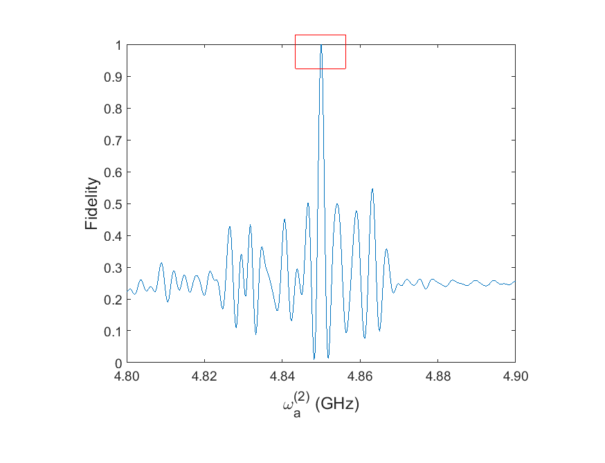
Figure 1: When uncertainty is not taken into account in optimization, the optimal solution produces a high fidelity for the simulated optimal value. However, away from the simulated value the fidelity rapidly drops off. The red square highlights how, at the optimum value, the fidelity value is 1 but drops off rapidly away from the value.

Sampling-based robust optimization takes a sample of points, $\delta_{i}$, from some range, $\Delta$, of the parameters that are uncertain Dong et al. (2014); Kosut et al. (2013). The fidelity is calculated from the time evolution of the Hamiltonian for each of the sampled parameter values, so that there is some range of fidelities, $\mathcal{F}_{i}$. Using this range of fidelities, the aim is then to either maximize the average fidelity of the range, or to maximize the worst-case value of fidelity in the range Kosut et al. (2013); Dong et al. (2014).

In general, for quantum computing, maximizing the average is not enough. If the average fidelity was maximized, there may exist a value in the range of uncertainty that performs far below the desired value. In this case, if the real system parameter has a value at this suboptimal value, then the actual performance of the gate would also be suboptimal. Indeed, in this situation, slow parameter drifts may often encounter adverse values of the parameter and thus degrade the fidelity over the duration of a quantum algorithm. If, instead, the worst-case fidelity were maximized for the range, then it would be guaranteed that all values in the range performed at least as well as this worst-case fidelity and ensure that the slow parameter drifts do not adversely affect the fidelity during operation. Therefore, maximizing the worst-case is the ideal target for quantum gates.

The numerical optimization algorithm used for this work is based on the Sequential Convex Programming (SCP) algorithm Kosut et al. (2013). This is a gradient-based, local search optimizer, similar in concept to GRAPE Khaneja et al. (2005). The SCP algorithm takes a piecewise constant approximation for the pulse shape, with the number of piecewise constant amplitudes determining the dimension of the control space. This algorithm is used to maximize a cost function of the form

$$\mathcal{F}=\bigg{|}\frac{1}{n_{s}}\mathrm{Tr}\big{(}W^{\dagger}\hat{O}U(T)\hat{O}\big{)}\bigg{|}^{2},$$ (5)

with $\hat{O}$ the projector into the computational subspace, $n_{s}$ the size of the computational subspace, $U(T)$ the time evolution of the full system at time $T$, and $W$ the desired unitary operator given by

$$W=\mathrm{exp}\bigg{(}-i\frac{\pi}{4}\sigma_{z}^{(1)}\sigma_{x}^{(2)}\bigg{)}.$$ (6)

This desired unitary operation is chosen as it is related to the CNOT operation via

$$\mathrm{CNOT}=\mathrm{exp}\bigg{(}i\frac{\pi}{4}\sigma_{z}^{(1)}\bigg{)}\mathrm{exp}\bigg{(}-i\frac{\pi}{4}\sigma_{z}^{(1)}\sigma_{x}^{(2)}\bigg{)}\mathrm{exp}\bigg{(}i\frac{\pi}{4}\sigma_{x}^{(2)}\bigg{)}.$$ (7)

At each iteration of the optimizer, SCP tries to find an optimal solution for the increment $\tilde{\varepsilon}$ from the linearized fidelities $\mathcal{F}(\varepsilon,\delta_{i})+\tilde{\varepsilon}\nabla_{\varepsilon}\mathcal{F}(\varepsilon,\delta_{i})$, where the control increment $\tilde{\varepsilon}$ satisfies some constraints and is within some predefined trust-region. Upon the return of this optimal $\tilde{\varepsilon}$ that satisfies all the constraints, the new fidelities are calculated and compared with the fidelities from the previous iteration. If $\mathrm{min}_{i}\mathcal{F}(\varepsilon+\tilde{\varepsilon},\delta_{i})>\mathrm{min}_{i}\mathcal{F}(\varepsilon,\delta_{i})$, then the control is updated to $\varepsilon\rightarrow\varepsilon+\tilde{\varepsilon}$, the trust region is increased and the optimization step is started again. If, however, $\mathrm{min}_{i}\mathcal{F}(\varepsilon+\tilde{\varepsilon},\delta_{i})<\mathrm{min}_{i}\mathcal{F}(\varepsilon,\delta_{i})$, then the trust region is instead decreased and the optimization step is repeated with $\varepsilon$ as the control again.

The key to the SCP algorithm is that the step to find the increment $\tilde{\varepsilon}$ is a convex optimizaton. In the optimization step, multiple instances of $\mathcal{F}(\varepsilon,\delta_{i})+\tilde{\varepsilon}\nabla_{\varepsilon}\mathcal{F}(\varepsilon,\delta_{i})$ are calculated for each sample parameter $\delta_{i}$ from the uncertain range. With these multiple instances, the optimal increment $\tilde{\varepsilon}$ is determined such that all of the $\mathcal{F}(\varepsilon,\delta_{i})+\tilde{\varepsilon}\nabla_{\varepsilon}\mathcal{F}(\varepsilon,\delta_{i})$ increase. This optimal increment is then inserted into the methodology described above to determine whether the new worst-case fidelity is greater than the previous worst-case fidelity. In the GRAPE algorithm, the method for increasing the fidelity via the gradient is to update the control via $\varepsilon_{k}\rightarrow\varepsilon_{k}+\alpha\partial\mathcal{F}/\partial\varepsilon_{k}$ where $k$ denotes the relevant piecewise constant amplitude in the control and $\alpha$ is some predefined increment. As the control is directly changed by inclusion of the gradient, the only way to include robustness is to calculate the average fidelity, e.g. $\mathcal{F}(\varepsilon)=\sum_{i=1}^{L}\mathcal{F}(\varepsilon,\delta_{i})$, and then use this for the gradient calculation and the update step. The update step then guarantees that the average fidelity is maximized and not the worst-case fidelity. Other works have discussed sampling-based optimization for robust control by maximizing the average fidelity Dong et al. (2014, 2016).

IV Time Optimization without Robustness

Before investigating robust optimal control with minimum time, it is instructive to look at the time minimization without robustness. As in almost all quantum control problems, solutions to time-optimization formulations are local. There are a variety of methods for finding local minimal time solutions, e.g. including the gate time in the cost function to penalize long gate times D’Alessandro (2007), or plotting the fidelity as a function of time Egger and Wilhelm (2013); Sorensen et al. (2016); Kirchhoff et al. (2018). Here the latter is used, where many random initial conditions for each time point are run and this process is repeated for all time points in the range. As the current resolution of state-of-the-art AWGs is 0.5 ns, this is chosen as the resolution of the time stepped control pulses. Therefore as time increases, so does the dimension of the control.

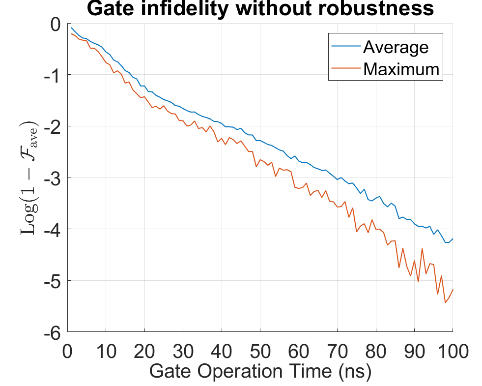
Figure 2: An SCP optimization algorithm is run without robustness for time points running from $1$ ns to $100$ ns, at each time point $20$ random initial guesses are made to start the optimization from. The figure displays the maximum and average infidelities reached for each time point out of the initial random starts.

To make the initial search the simulations are run for each time points from $1$ ns to $100$ ns, in increments of $1$/,ns. For every time point, $20$ random guesses are made for the initial starting point for the search; the SCP algorithm is then run until either the maximum number of iterations is reached or the maximum fidelity for that search is reached. Figure 2 displays a logarithmic plot of the infidelity of the maximum and average fidelity of the 20 randoms runs against the time of the gate.

Figure 3 shows that after $40$ ns the maximum and average fidelities at all time points are $\mathcal{F}>0.99$. Further, after  $80$ ns the maximum fidelity is $\mathcal{F}>0.9999$, while after  $95$ ns the average fidelity is also $\mathcal{F}>0.9999$. Comparing with the state-of-the-art implementation in Sheldon et al. (2016) this is approximately a factor 4 improvement in the duration of the gate for the same fidelity with a higher fidelity value achievable in less the $100$ ns; a value that is important for fault-tolerant quantum computation Aharonov and Ben-Or (2008).

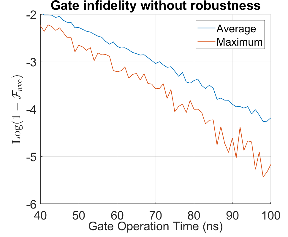
Figure 3: A closer view of the results in Figure 2, showing that for each time point after $40$ ns the fidelity $\mathcal{F}>0.99$. Additionally, after approximately $80$ ns all the maximum fidelity values $\mathcal{F}>0.9999$, while this achieved for the average values after approximately $95$ ns.

V Time Optimization with Robustness

In order to perform the search including robustness, the same search is carried out as before, namely the SCP algorithm is run with 20 different initial starting points for each time points from $1$ ns to $100$ ns. For the robust search, each simulation includes some error in the Hamiltonian and the robustness method is applied. In general, the dominant uncertainty in the Hamiltonian is the coupling strength $J$; this is due to the way in which it is measured and estimated.

(a) The average infidelity for varying uncertainty is plotted against the operation time of the gate from $1$ ns to $100$ ns.

(b) A closer view of 4a showing the time taken to achieved fidelities $\mathcal{F}>0.99$ and higher.

Figure 4: The optimization is run with uncertainty in the $J$ coupling ranging from 1% uncertainty to 10% uncertainty. At each time point the average worst-case infidelity from the random starts is displayed. The figure shows that within a time of $52$ ns a robust pulse can be achieved with an average worst-case fidelity $\bar{\mathcal{F}_{\mathrm{min}}}>0.99$ for uncertainty up to 10%. The graphs further show that the range of uncertainty becomes important for the achievable fidelity as the infidelity curves begin to flatten out, with only uncertainty less than 10% achieving $\mathcal{F}>0.999$.

The search described above is performed for a varying size of error in the coupling strength $J$, ranging from no error up to $10\%$ error. Figure 4 shows that, with up to 10% error in the system, the optimizer has found pulses that can achieve a fidelity of $\mathcal{F}>0.99$ in approximately $52$ ns. While this is $12$ ns slower than for the no robustness case, this is still a factor of 3 faster than the state-of-the-art gate in Sheldon et al. (2016). Additionally, it can be seen that for uncertainty levels up to $3\%$, fidelities of $\mathcal{F}>0.999$ can be achieved in times of less than approximately $77$ ns. At these short times decoherence will be at a minimum, if not negligible, as most transmon qubits have coherence times in the $10$’s of microseconds Sheldon et al. (2016), while the state-of-the-art is around $0.1$ ms Rigetti et al. (2012).

Figure 4 shows that the fidelities tend to some value for each size of uncertainty. For uncertainties greater than $3\%$, the fidelities tend to values less than $\mathcal{F}=0.999$, within the constraints of the system that has been simulated. This suggests that the optimal level of uncertainty for this system is $3\%$ or less; if this level of measurement uncertainty for the $J$ coupling can be reached, then high fidelity short robust pulses can be achieved.

VI Classical Control Crosstalk

In the previous two sections the idealized situation in which the control on one qubit does not directly drive the other qubit has been considered. However, in reality there may be some amount of classical crosstalk due to the way in which the control drives are brought in to the circuit. This classical crosstalk manifests itself as the drive of one qubit directly driving the other qubit with some weighting dependent on the coupling of the drive with the other qubit Chow et al. (2011).

In order to model classical crosstalk, the control term in line 3 of eqn. II is expanded to include terms that represent the classical coupling of the control drive for one qubit to the other qubit

$$H_{c}=\sum_{\begin{subarray}{c}i,j=1,2\\ i\neq j\end{subarray}}\bigg{(} \varepsilon_{j}^{x}(t)\Big{(}\big{(}b^{\dagger}_{j}+b_{j}\big{)}+\alpha_{j}\big{(}b^{\dagger}_{i}+b_{i}\big{)}\Big{)}$$

$$+i\varepsilon_{j}^{y}(t)\Big{(}\big{(}b_{j}^{\dagger}-b_{j}\big{)}+\alpha_{j}\big{(}b_{i}^{\dagger}-b_{i}\big{)}\Big{)}\bigg{)}.$$ (8)

Here, $\alpha_{j}$ represents the coupling of the drive on qubit $j$ with qubit $i$.

As with the previous situation, it is instructive to look at the situation in which there are no uncertainties in the system. Figure 5 shows this compared with the results shown in Figure 2 where $\alpha_{j}$ is chosen as $\alpha_{1}=\alpha_{2}=0.1$, which is a non-trivial and realistic amount of crosstalk in the system. Although it was considered that this level of crosstalk involved in the Hamiltonian is sub-optimal, Figure 5 shows that the crosstalk case very closely follows the results where there was no crosstalk.

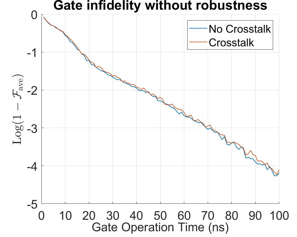
Figure 5: A comparison of the average infidelities when there is classical crosstalk within the system versus the case when there are only direct drives with no crosstalk. In this case 10% of the pulse is affecting the other qubit. It is noted that this amount of crosstalk does not inhibit the optimizer from finding high fidelity solutions.

Figure 6 displays the average infidelity against time for the multiple random starts, following the same search method as described above. The graph shows that within a time of approximately $55$ ns, all the error ranges achieve an average worst-case fidelity of $\mathcal{F}=0.99$. This is only marginally slower than for the no crosstalk situation, which achieves the result in a time of approximately $52$ ns. As with the no crosstalk case, Figure 6 further shows that the optimal level of uncertainty for fast gate operation times is less the $3\%$ as fidelities of $\mathcal{F}>0.999$ can be achieved with this maximum level of uncertainty in times less than $80$ ns.

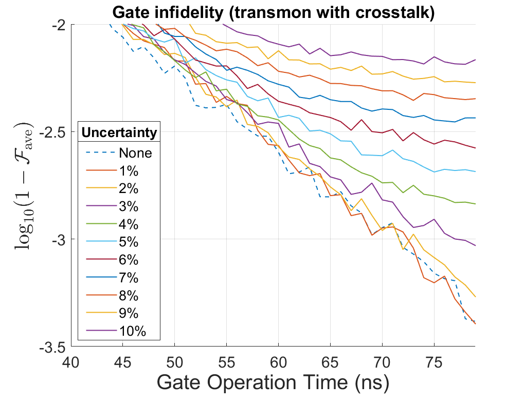
Figure 6: The level of infidelity of a robust optimal pulse where a level of 10% crosstalk is assumed. The figure shows that within a time of $55$ ns a robust pulse can be achieved with an average worst-case fidelity $\bar{\mathcal{F}_{\mathrm{min}}}>0.99$, with uncertainty up to 10%. This is extremely close to the time for the no crosstalk situation. Additionally, the optimum level of uncertainty is less then $3$% as fidelities $\mathcal{F}>0.999$ are achievable.

The above shows extremely promising results for a robust cross-resonance gate in multi-level devices. In both cases, with and without crosstalk, robust pulses are achieved with average worst-case fidelities $\mathcal{F}>0.99$ in times of less then $60$ ns. This is approximately a factor of 3 speed up on the state-of-the-art implementation of cross resonance gates. The inclusion of crosstalk makes the results more experimentally relevant, while further restricting the piecewise constant amplitudes to $2$ ns resolution (the limit of current state-of-the-art AWGs) further adds weight to the promising results for future experiments.

VII Two-level qubits

While multi-level qubits with weak anharmonic structures are currently widely used in many superconducting research groups, work is still being progressed in qubits with more isolated two-level structures where the non-computational levels are far enough away that there is no significant leakage out of the computational subspace Mooij et al. (1999); Orlando et al. (1999); van der Wal et al. (2000); Chiorescu et al. (2003); Yoshihara et al. (2006); Bylander et al. (2011); Stern et al. (2014). As all the dynamics during the gate operation are contained within the computational subspace, it would indicate that two-level systems would be the preferable choice for the cross-resonance gate and should achieve higher fidelity, shorter gate times due to the lack of leakage.

To simulate two-level qubits, eqn. II is adapted with reduced dimensions down to two levels for each qubit to effectively consider two two-level systems. With this alteration, the same initial search is performed as previously with no uncertainty in the system in order to give an indication of the minimal time for the two-level qubits. Figure 7 displays the results of this search and compares them with the multi-level case, which displays a somewhat unexpected and interesting feature. For the two-level qubit case, as expected, fidelities at the lower times are higher than for the multi-level qubits. It is expected that the limiting factor is the leakage levels where the potentially large amplitude pulses are driving these higher level interactions and limiting the fidelity. However, as the time is increased the fidelities increase more gradually for the two-level qubits than for the multi-level qubits. Eventually the fidelities of the multi-level qubits become higher than the two-level qubits for the same time values. Figure 7 further shows that multi-level qubits reach fidelity values of $\mathcal{F}>0.99$ in times of approximately $T\geq 40$ ns, whereas for two-level qubits this is achieved for $T\geq 58$ ns.

Figure 7: A comparison of the performance of two-level qubits, multi-level qubits with no crosstalk, and multi-level qubits with crosstalk, where the average infidelity for each time point is plotted. Initially the two-level qubit simulations produce higher fidelity pulses initially. However, the improvement in fidelity for the two-level qubits is more gradual than for the multi-level qubits, with the multi-level qubits achieving higher fidelities in shorter time than the two-level qubits. This suggests that the third level is being used during the pulse time to gain higher fidelities.

This feature, where the fidelities for the multi-level qubits are greater than for the two-level qubits and tend towards higher fidelities more quickly, suggests that the third level is actively used during the gate operation. Figure 8 shows plots of the value $1-|\mathrm{tr}(\prod_{k}U_{k}^{\dagger}\hat{O}\prod_{k}U_{k}\hat{O})|^{2}/d^{2}$ for each time point $k$ within the pulse length for gate operation times of $T=10,20,40,80$ ns. This gives a representation of the leakage for each of the pulses, where it is assumed that leakage $=1-|\mathrm{tr}(\prod_{k}U_{k}^{\dagger}\hat{O}\prod_{k}U_{k}\hat{O})|^{2}/d^{2}$. $\hat{O}$ is the projection operator into the four-level two-qubit subspace and $d=2$ for the qubit case. $|\mathrm{tr}(\prod_{k}U_{k}^{\dagger}\hat{O}\prod_{k}U_{k}\hat{O})|^{2}/d^{2}$ would be unity if there was no leakage from the qubit subspace, and therefore the graphs display the level of leakage out of the computational subspace.

Figure 8 shows that for each of the pulse length times there is a significant degree of leakage during the operation, suggesting that the third level is extremely important for these pulse shapes and eventually the higher fidelities that are able to be achieved in the multi-level cases.

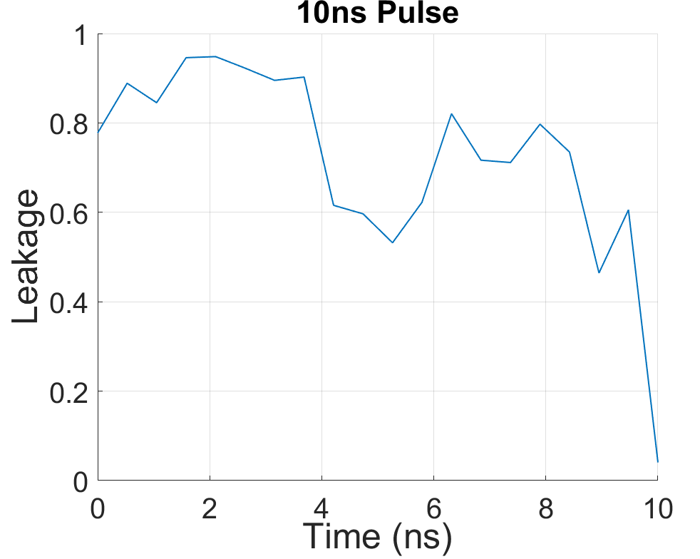
(a) Representation of leakage for $10$ ns pulse.

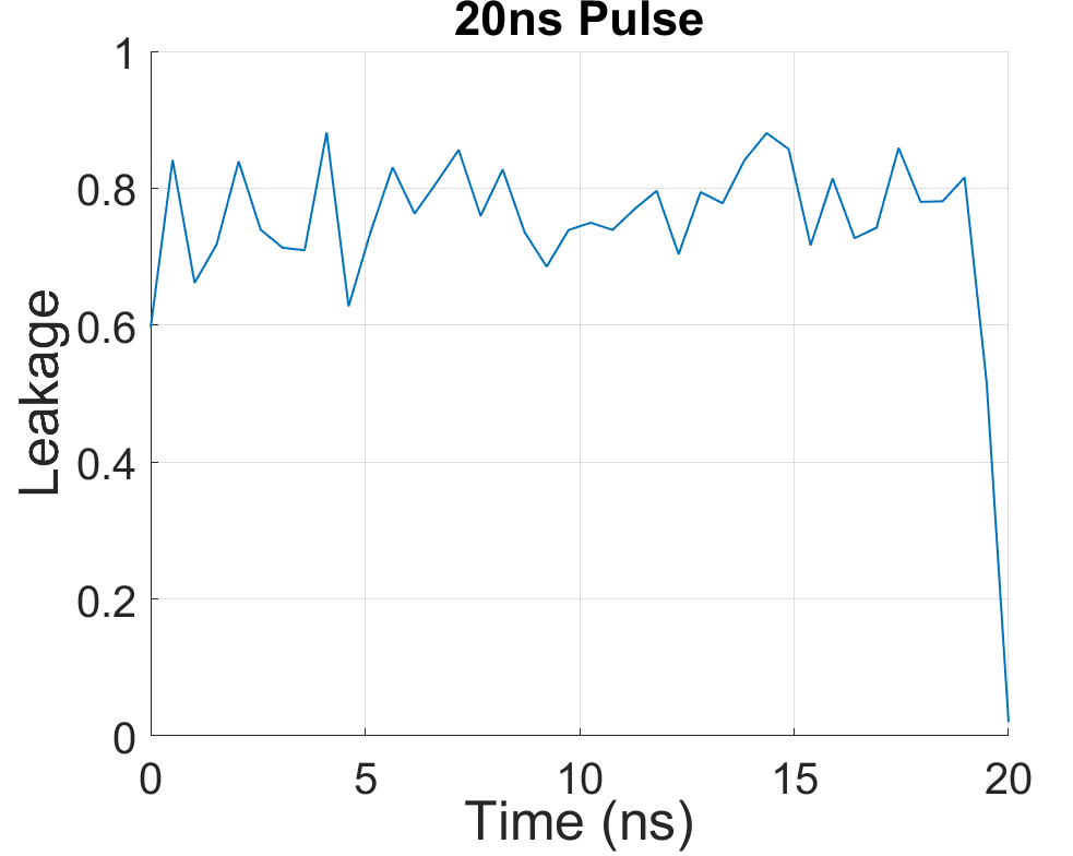
(b) Representation of leakage for $20$ ns pulse.

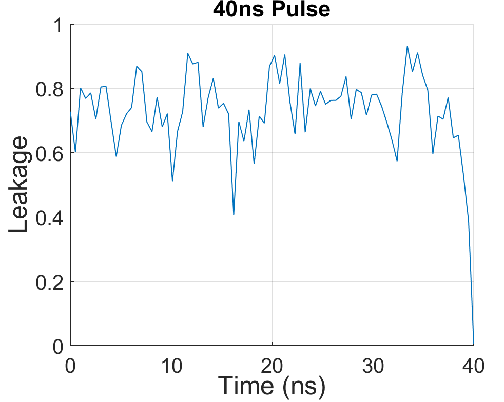
(c) Representation of leakage for $40$ ns pulse.

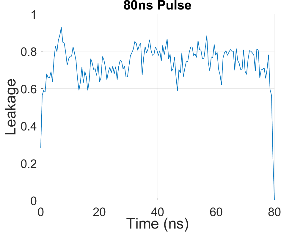
(d) Representation of leakage for $80$ ns pulse.

Figure 8: For each of the pulse length times chosen above, the value $|\mathrm{tr}(\prod_{k}U_{k}^{\dagger}\prod_{k}U_{k})|^{2}/d^{2}$ is calculated at each time point, $k$, during the pulse. This then determines how unitary the evolution operator is at that time point, which indicates how much leakage there is at that time point. It is assumed leakage $=1-|\mathrm{tr}(\prod_{k}U_{k}^{\dagger}\prod_{k}U_{k})|^{2}/d^{2}$, where $d=4$ for a two-qubit ideal system.

Figure 9 shows the fidelities with time for the robust pulses for the two-level qubits. Similar to the multi-level system case the trend is the same as the no uncertainty case, with the fidelities decreasing for each increase in uncertainty. In this case, Figure 9 shows that after a time of $T=70$ ns average fidelities of $\mathcal{F}>0.99$ are achieved for all ranges of uncertainty up to $10\%$. This is again a speed up of gate time compared with current state-of-the-art implementation. For the two-level qubits, however, the trend of the fidelities shows that the optimal level uncertainty is less than $4\%$, as opposed to the $3\%$ for the multi-level qubits. In a time of approximately $95$ ns, fidelities of $\mathcal{F}>0.999$ are achievable with uncertainty up to $4\%$.

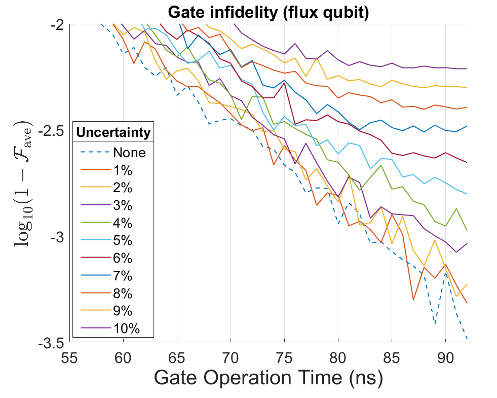
Figure 9: Average worst-case infidelity is given for the two-level qubit optimization. The figure shows that within a time of $70$ ns a robust pulse can be achieved with an average worst-case fidelity $\bar{\mathcal{F}_{\mathrm{min}}}>0.99$, with uncertainty up to 10%. This is longer than for the multi-level qubits and suggests more third level interactions.

VIII Conclusion

We have shown that the robust SCP algorithm can achieve robust pulses with fidelities $\mathcal{F}>0.99$ in a time of approximately 55 ns for multi-level systems and approximately $70$ ns for two-level qubit systems. This is a factor of three faster than the current state-of-the-art implementation for the multi-level case and a factor of two faster for two-level case Sheldon et al. (2016); this is while being robust to one of the most uncertain parameters in the system, the $J$ coupling. Fidelities of $\mathcal{F}=0.99$ are suitable for surface code quantum error correction Bravyi and Kitaev ; Fowler et al. (2009, 2012); this is ideal as there has been much work looking towards implementing surface codes in superconducting qubit devices Barends et al. (2014); Versluis et al. (2017); Córcoles et al. (2015); Simonite (2016); Gambetta et al. (2017). The robustness of the results also ensures there is less variability in the performance in multi-qubit processors which is ideal for scaling up quantum computers. We have further shown that for short gate times there is an optimal level of uncertainty for each of the devices. For the multi-level qubits, uncertainty levels up to $3\%$ can achieve fidelities $\mathcal{F}>0.999$ in gates times of $75$ ns. For two-level qubits, uncertainty levels up to $4\%$ can achieve fidelities $\mathcal{F}>0.999$ in gates times of 95 ns.

It has also been shown that, in theory, the coupled multi-level qubits can outperform the coupled two-level qubit systems; the addition of a third level can allow for more complicated dynamics and give an extra dimension to be used during the operation. This has led to a faster convergence of higher fidelity results for the multi-level qubits when compared with the two-level qubits, achieving fidelities $\mathcal{F}>0.99$ in a time of $15$ ns faster. However, care must be taken when considering this result as the simulations were limited to just the three level system and no other dynamics. In this case of two closed three-level systems, the excitations can return to the computational basis. In reality this may not be the case and the fidelities given may be lower due to permanent loss from the computational basis. Further work should look to include higher levels than the third to accurately give a result for transmons. Nonetheless, these results show promise for transmons. Additionally, there are certain multi-level superconducting qutrits for which these results could be directly applicable Fedorov et al. (2012); Bækkegaard et al. (2018). Nitrogen-vacancy centres could also benefit from these results as the level structure is more like a three-level system with the fourth level being far away Childress et al. (2006), similar to the simulations in this paper.

While the best achievable fidelities are limited by uncertainty (for the case of constant piecewise control lengths of $0.5$ ns), the results nonetheless show that uncertainty can be dealt with if a certain duration of gate time is accepted. Given the current interest in noise intermediate-scale quantum (NISQ) technologies Preskill (2018), the results also show that shorter gate times on the order of $30$ ns can be implemented for the full range of uncertainty using our parameterization if lower fidelities can be accepted. This gate time would give fidelities of approximately $\mathcal{F}=0.96$ for all cases, which is what NISQ technologies are targeting as a minimum gate fidelity for implementation.

*

Appendix A Pulse Examples

Figures 10, 11 and 12 show pulses with an operation time of $75$ ns for all the cases investigated with and without robustness. Each pulse achieves the best or best worst-case fidelity for the operation time of $75$ ns. Here, $c_{1}(t)=\varepsilon_{1}^{x}(t)$, $c_{2}(t)=\varepsilon_{1}^{y}(t)$, $c_{3}(t)=\varepsilon_{2}^{x}(t)$, $c_{4}(t)=\varepsilon_{2}^{y}(t)$.

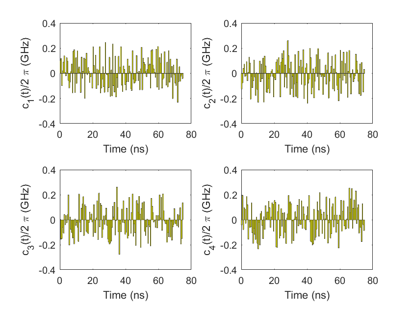
(a) Pulse that achieves the best fidelity for an operation time of $75$ ns. The fidelity achieved is $\mathcal{F}=0.9999$.

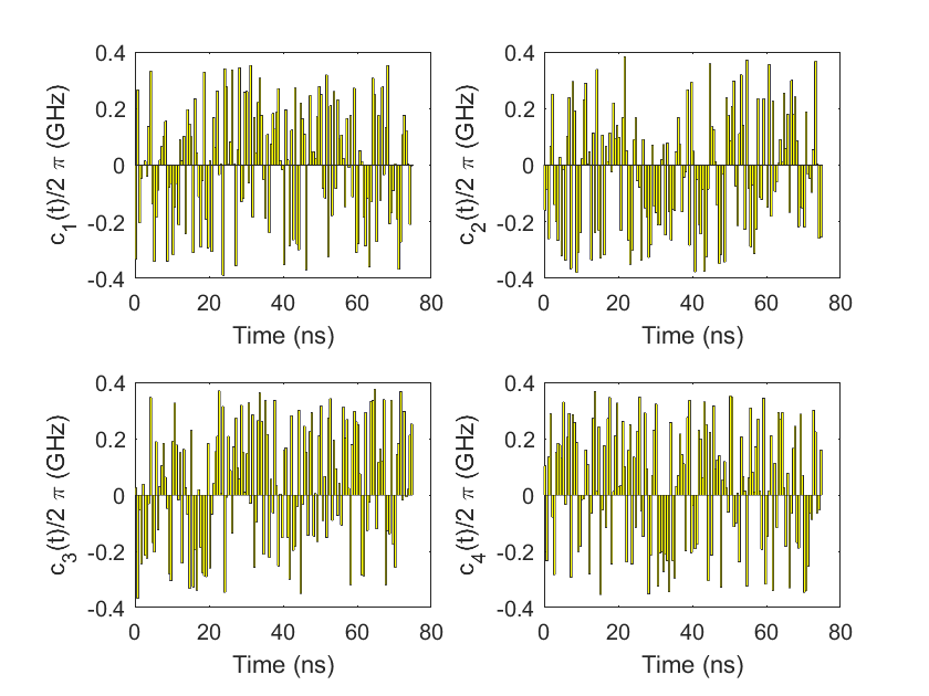
(b) Robust pulse that achieves the best worst-case fidelity for an uncertainty size of $\pm 10$ ns. The worst-case fidelity achieved is $\mathcal{F}=0.9949$.

Figure 10: Example pulses for the optimization simulation with and without robustness. The operation for both pulses is $75$ ns. The pulses displayed achieve the best fidelity, or best worst-case fidelity for the robust pulses, out of the multiple start simulations.

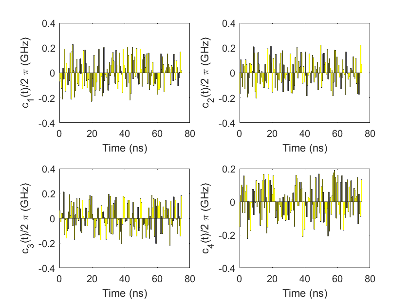
(a) Pulse that achieves the best fidelity when there is crosstalk. The fidelity achieved is $\mathcal{F}=0.9998$.

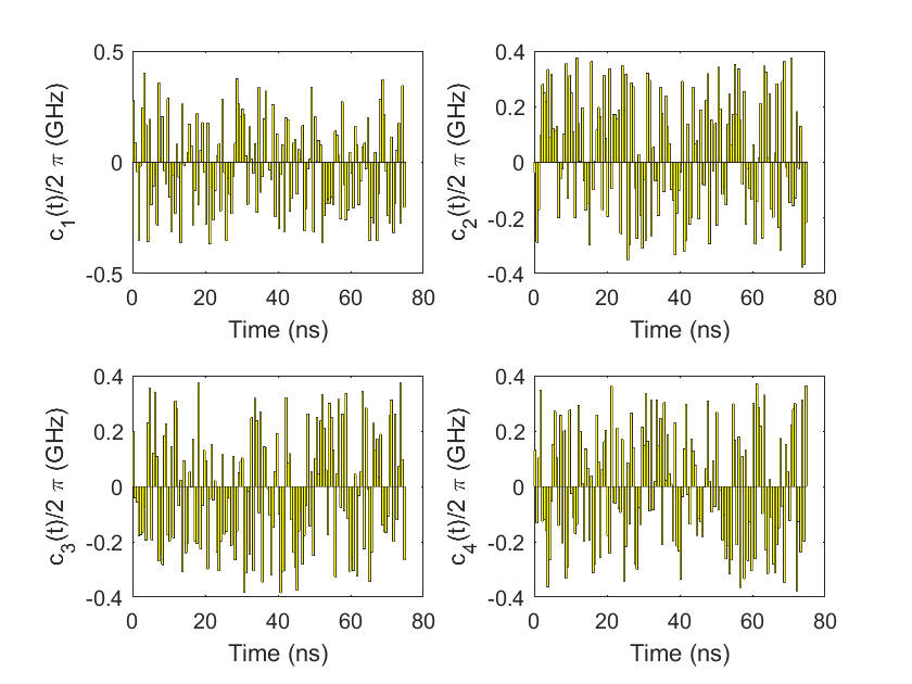
(b) Robust pulse that achieves the best worst-case fidelity for an uncertainty size of $\pm 10$ ns when there is crosstalk. The worst-case fidelity achieved is $\mathcal{F}=0.9943$.

Figure 11: Example pulses for the optimization simulation with and without robustness with crosstalk present. The operation for both pulses is $75$ ns. The pulses displayed achieve the best fidelity, or best worst-case fidelity for the robust pulses, out of the multiple start simulations.

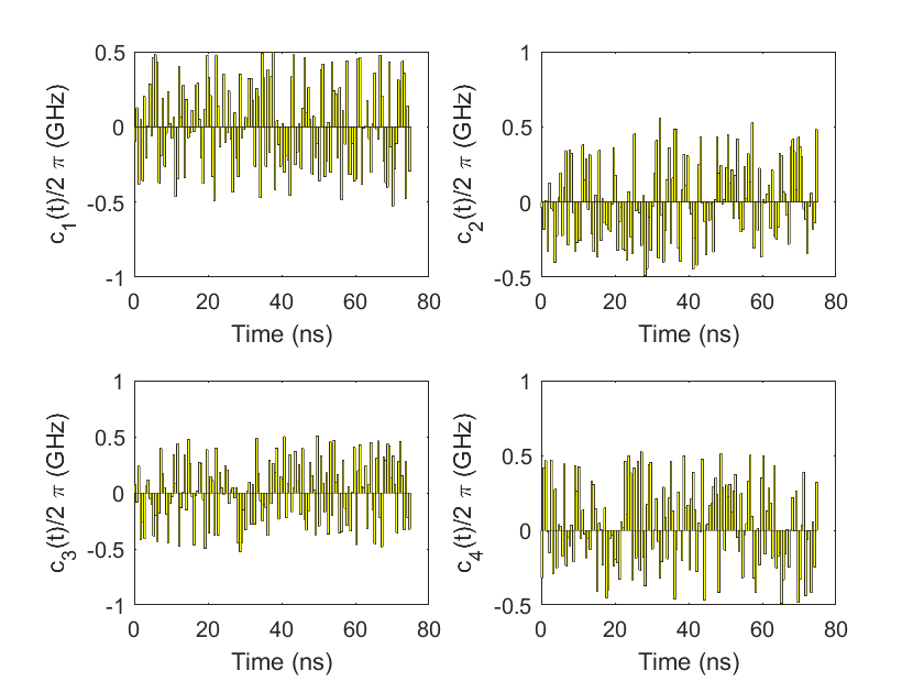
(a) Pulse that achieves the best fidelity for flux qubits. The fidelity achieved is $\mathcal{F}=0.9999$.

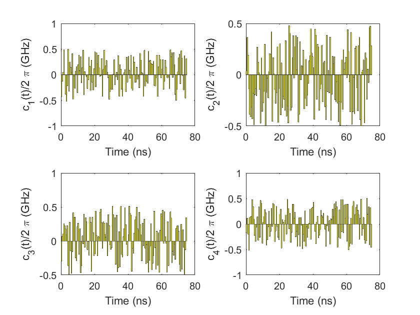
(b) Robust pulse that achieves the best worst-case fidelity for an uncertainty size of $\pm 10$ ns for flux qubits. The worst-case fidelity achieved is $\mathcal{F}=0.9939$.

Figure 12: Example pulses for the optimization simulation with and without robustness or flux qubits. The operation for both pulses is $75$ ns. The pulses displayed achieve the best fidelity, or best worst-case fidelity for the robust pulses, out of the multiple start simulations.

References

- Blais et al. (2004) A. Blais, R.-S. Huang, A. Wallraff, S. M. Girvin, and R. J. Schoelkopf, Phys. Rev. A 69, 062320 (2004).
- Blais et al. (2007) A. Blais, J. Gambetta, A. Wallraff, D. I. Schuster, S. M. Girvin, M. H. Devoret, and R. J. Schoelkopf, Phys. Rev. A 75, 032329 (2007).
- Gu et al. (2017) X. Gu, A. F. Kockum, A. Miranowicz, Y. xi Liu, and F. Nori, Physics Reports 718-719, 1 (2017), microwave photonics with superconducting quantum circuits.
- Aharonov and Ben-Or (2008) D. Aharonov and M. Ben-Or, SIAM J. Comput. 38, 1207 (2008).
- Barends et al. (2014) R. Barends, J. Kelly, A. Megrant, A. Veitia, D. Sank, E. Jeffrey, T. C. White, J. Mutus, A. G. Fowler, B. Campbell, Y. Chen, Z. Chen, B. Chiaro, A. Dunsworth, C. Neill, P. O’Malley, P. Roushan, A. Vainsencher, J. Wenner, A. N. Korotkov, A. N. Cleland, and J. M. Martinis, Nature 508, 500 (2014).
- Levitin et al. (2002) L. B. Levitin, T. Toffoli, and Z. Walton (2002).
- Svozil et al. (2005) K. Svozil, L. Levitin, T. Toffoli, and Z. Walton, International Journal of Theoretical Physics 44, 965 (2005).
- Carlini et al. (2006) A. Carlini, A. Hosoya, T. Koike, and Y. Okudaira, Phys. Rev. Lett. 96, 060503 (2006).
- Carlini et al. (2007) A. Carlini, A. Hosoya, T. Koike, and Y. Okudaira, Phys. Rev. A 75, 042308 (2007).
- Ashhab et al. (2012) S. Ashhab, P. C. de Groot, and F. Nori, Phys. Rev. A 85, 052327 (2012).
- Lee et al. (2018) J. Lee, C. Arenz, H. Rabitz, and B. Russell, New Journal of Physics 20, 063002 (2018).
- Ginossar et al. (2010) E. Ginossar, L. S. Bishop, D. I. Schuster, and S. M. Girvin, Phys. Rev. A 82, 022335 (2010).
- Goerz et al. (2017) M. H. Goerz, F. Motzoi, K. B. Whaley, and C. P. Koch, NPJ Quantum Information 3, 37 (2017).
- Goetz et al. (2016) R. E. Goetz, A. Karamatskou, R. Santra, and C. P. Koch, Phys. Rev. A 93, 013413 (2016).
- Cross and Gambetta (2015) A. W. Cross and J. M. Gambetta, Phys. Rev. A 91, 032325 (2015).
- Theis et al. (2016a) L. S. Theis, F. Motzoi, F. K. Wilhelm, and M. Saffman, Phys. Rev. A 94, 032306 (2016a).
- Schöndorf et al. (2018) M. Schöndorf, L. C. G. Govia, M. G. Vavilov, R. McDermott, and F. K. Wilhelm, Quantum Science and Technology 3, 024009 (2018).
- Liebermann and Wilhelm (2016) P. J. Liebermann and F. K. Wilhelm, Phys. Rev. Applied 6, 024022 (2016).
- Theis et al. (2016b) L. S. Theis, F. Motzoi, and F. K. Wilhelm, Phys. Rev. A 93, 012324 (2016b).
- Machnes et al. (2018) S. Machnes, E. Assémat, D. Tannor, and F. K. Wilhelm, Phys. Rev. Lett. 120, 150401 (2018).
- Egger and Wilhelm (2013) D. Egger and F. K. Wilhelm, Supercond. Sci. Tehnol. 27, 014001 (2013).
- Egger and Wilhelm (2014) D. J. Egger and F. K. Wilhelm, Phys. Rev. Lett. 112, 240503 (2014).
- Kosut et al. (2013) R. L. Kosut, M. D. Grace, and C. Brif, Phys. Rev. A 88, 052326 (2013).
- Goerz et al. (2014) M. H. Goerz, E. J. Halperin, J. M. Aytac, C. P. Koch, and K. B. Whaley, Phys. Rev. A 90, 032329 (2014).
- Dong et al. (2014) D. Dong, C. Chen, B. Qi, I. R. Petersen, and F. Nori, Sci. Rep. 5, 7873 (2014).
- Allen et al. (2017) J. L. Allen, R. Kosut, J. Joo, P. Leek, and E. Ginossar, Phys. Rev. A 95, 042325 (2017).
- Rigetti and Devoret (2010) C. Rigetti and M. Devoret, Phys. Rev. B 81, 134507 (2010).
- Chow et al. (2011) J. M. Chow, A. D. Córcoles, J. M. Gambetta, C. Rigetti, B. R. Johnson, J. A. Smolin, J. R. Rozen, G. A. Keefe, M. B. Rothwell, M. B. Ketchen, and M. Steffen, Phys. Rev. Lett. 107, 080502 (2011).
- Reagor et al. (2016) M. Reagor, W. Pfaff, C. Axline, R. W. Heeres, N. Ofek, K. Sliwa, E. Holland, C. Wang, J. Blumoff, K. Chou, M. J. Hatridge, L. Frunzio, M. H. Devoret, L. Jiang, and R. J. Schoelkopf, Phys. Rev. B 94, 014506 (2016).
- Koch et al. (2007) J. Koch, T. M. Yu, J. Gambetta, A. A. Houck, D. I. Schuster, J. Majer, A. Blais, M. H. Devoret, S. M. Girvin, and R. J. Schoelkopf, Physical Review A 76, 042319 (2007).
- Sheldon et al. (2016) S. Sheldon, E. Magesan, J. M. Chow, and J. M. Gambetta, Phys. Rev. A 93, 060302(R) (2016).
- Nielsen and Chuang (2010) M. A. Nielsen and I. L. Chuang, Quantum Computation and Quantum Information, 10th ed. (Cambridge University Press, 2010).
- Kirchhoff et al. (2018) S. Kirchhoff, T. Keßler, P. J. Liebermann, E. Assémat, S. Machnes, F. Motzoi, and F. K. Wilhelm, Phys. Rev. A 97, 042348 (2018).
- Economou and Barnes (2015) S. E. Economou and E. Barnes, Phys. Rev. B 91, 161405(R) (2015).
- Barnes et al. (2017) E. Barnes, C. Arenz, A. Pitchford, and S. E. Economou, Phys. Rev. B 96, 024504 (2017).
- Majer et al. (2007) J. Majer, J. M. Chow, J. M. Gambetta, J. Koch, B. R. Johnson, J. A. Schreier, L. Frunzio, D. I. Schuster, A. A. Houck, A. Wallraff, A. Blais, M. H. Devoret, S. M. Girvin, and R. J. Schoelkopf, Nature 449, 443 (2007), 0709.2135 .
- de Groot et al. (2012) P. C. de Groot, S. Ashhab, A. Lupaşcu, L. DiCarlo, F. Nori, C. J. P. M. Harmans, and J. E. Mooij, New Journal of Physics 14, 073038 (2012).
- Khaneja et al. (2005) N. Khaneja, T. Reiss, C. Kehlet, T. Schulte-Herbruggen, and S. J. Glaser, J. Magn. Reson. 172, 296 (2005).
- Dong et al. (2016) D. Dong, C. Wu, C. Chen, B. Qi, I. R. Petersen, and F. Nori, Scientific Reports 6, 1 (2016).
- D’Alessandro (2007) D. D’Alessandro, Introduction to Quantum Control and Dynamics (Chapman and Hall, 2007).
- Sorensen et al. (2016) J. J. W. H. Sorensen, M. K. Pedersen, M. Munch, P. Haikka, J. H. Jensen, T. Planke, M. G. Andreasen, M. Gajdacz, K. Mølmer, A. Lieberoth, and J. F. Sherson, Nature 532, 210 (2016).
- Rigetti et al. (2012) C. Rigetti, J. M. Gambetta, S. Poletto, B. L. T. Plourde, J. M. Chow, A. D. Córcoles, J. A. Smolin, S. T. Merkel, J. R. Rozen, G. A. Keefe, M. B. Rothwell, M. B. Ketchen, and M. Steffen, Phys. Rev. B 86, 100506(R) (2012).
- Mooij et al. (1999) J. E. Mooij, T. P. Orlando, L. Levitov, L. Tian, C. H. van der Wal, and S. Lloyd, Science 285, 1036 (1999).
- Orlando et al. (1999) T. P. Orlando, J. E. Mooij, L. Tian, C. H. van der Wal, L. S. Levitov, S. Lloyd, and J. J. Mazo, Phys. Rev. B 60, 15398 (1999).
- van der Wal et al. (2000) C. H. van der Wal, A. C. J. ter Haar, F. K. Wilhelm, R. N. Schouten, C. J. P. M. Harmans, T. P. Orlando, S. Lloyd, and J. E. Mooij, Science 290, 773 (2000).
- Chiorescu et al. (2003) I. Chiorescu, Y. Nakamura, C. J. P. M. Harmans, and J. E. Mooij, Science 299, 1869 (2003).
- Yoshihara et al. (2006) F. Yoshihara, K. Harrabi, A. O. Niskanen, Y. Nakamura, and J. S. Tsai, Phys. Rev. Lett. 97, 167001 (2006).
- Bylander et al. (2011) J. Bylander, S. Gustavsson, F. Yan, F. Yoshihara, K. Harrabi, G. Fitch, D. G. Cory, Y. Nakamura, J. Tsai, and W. D. Oliver, Nature Physics 7, 565 (2011).
- Stern et al. (2014) M. Stern, G. Catelani, Y. Kubo, C. Grezes, A. Bienfait, D. Vion, D. Esteve, and P. Bertet, Phys. Rev. Lett. 113, 123601 (2014).
- (50) S. Bravyi and A. Y. Kitaev, arXiv:quant-ph/9811052 .
- Fowler et al. (2009) A. G. Fowler, A. M. Stephens, and P. Groszkowski, Phys. Rev. A 80, 052312 (2009).
- Fowler et al. (2012) A. G. Fowler, M. Mariantoni, J. M. Martinis, and A. N. Cleland, Phys. Rev. A 86, 032324 (2012).
- Versluis et al. (2017) R. Versluis, S. Poletto, N. Khammassi, B. Tarasinski, N. Haider, D. J. Michalak, A. Bruno, K. Bertels, and L. DiCarlo, Phys. Rev. Applied 8, 034021 (2017).
- Córcoles et al. (2015) A. Córcoles, E. Magesan, S. J. Srinivasan, A. W. Cross, M. Steffen, J. M. Gambetta, and J. M. Chow, Nature Communications 6, 6979 (2015).
- Simonite (2016) T. Simonite, TECHNOLOGY REVIEW 119, 17 (2016).
- Gambetta et al. (2017) J. M. Gambetta, J. M. Chow, and M. Steffen, npj Quantum Information 3, 2 (2017).
- Fedorov et al. (2012) A. Fedorov, L. Steffen, M. Baur, M. P. da Silva, and A. Wallraff, Nature 481, 170 (2012).
- Bækkegaard et al. (2018) T. Bækkegaard, L. Kristensen, N. Loft, C. Andersen, D. Petrosyan, and N. Zinner, (2018), arXiv:1802.04299 .
- Childress et al. (2006) L. Childress, M. V. Gurudev Dutt, J. M. Taylor, A. S. Zibrov, F. Jelezko, J. Wrachtrup, P. R. Hemmer, and M. D. Lukin, Science 314, 281 (2006), http://science.sciencemag.org/content/314/5797/281.full.pdf .
- Preskill (2018) J. Preskill, Quantum 2, 79 (2018).
*